SynxDB 2 Documentation
This site provides complete documentation for SynxDB 2, a high-performance, open-source MPP (Massively Parallel Processing) database designed for large-scale analytics. SynxDB is an enterprise-grade database with a scalable architecture, and can act as a drop-in replacement for Greenplum 6 to seamless migration without change your existing workloads.
Note Greenplum® is a registered trademark of Broadcom Inc. Synx Data Labs and SynxDB are not affiliated with, endorsed by, or sponsored by Broadcom, Inc. Any references to Greenplum are for comparative, educational, and interoperability purposes only.
Quick-Start Installation
This guide provides simple instructions for installing SynxDB 2 on a host machine.
Note For detailed instructions on preparing host machines and deploying SynxDB in a production environment, see Installing and Upgrading SynxDB.
Security Considerations
The installation procedure follows a structured RPM-based approach, similar to EPEL, in order to secure dependency management and updates. Synx Data Labs maintains high security standards through:
- Cryptographically signed RPM packages
- Signed repository metadata
- GPG key verification
- Package signature validation at multiple stages
All artifacts used in the installation process are cryptographically signed to ensure package integrity and authenticity.
Prerequisites
To install SynxDB you require:
- A supported EL9-compatible operating system (RHEL 9, Rocky Linux 9, Oracle Linux 9, AlmaLinux 9) or EL8-compatible operating system (RHEL 8, Rocky Linux 8, Oracle Linux 8, AlmaLinux 8), or EL8-compatible operating system (RHEL 7, CentOS 7).
rootaccess to each host system. This procedure assumes that you are logged in as therootuser. As an alternative, prependsudoto each command if you choose to install as a non-root user.- The
wgetutility. If necessary installwgeton each host with the command:dnf install wget - Internet access to Synx Data Labs repositories. This guide assumes that each host can access the Synx Data Labs repositories. If your environment restricts internet access, or if you prefer to host repositories within your infrastructure to ensure consistent package availability, contact Synx Data Labs to obtain a complete repository mirror for local hosting.
Procedure
Follow these steps to securely install SynxDB to your system:
-
Login to your Enterprise Linux 8 or 9 system as the
rootuser. -
Import the Synx Data Labs GPG key so you can use it to validate downloaded packages:
wget -nv https://synxdb-repo.s3.us-west-2.amazonaws.com/gpg/RPM-GPG-KEY-SYNXDB rpm --import RPM-GPG-KEY-SYNXDB -
Verify that you have imported the keys:
rpm -q gpg-pubkey --qf "%{NAME}-%{VERSION}-%{RELEASE} %{SUMMARY}\n" | grep SynxDBYou should see output similar to:
gpg-pubkey-df4bfefe-67975261 gpg(SynxDB Infrastructure <infrastructure@synxdata.com>) -
Download the SynxDB repository package:
wget -nv https://synxdb-repo.s3.us-west-2.amazonaws.com/repo-release/synxdb2-release-1-1.rpm -
Verify the package signature of the repository package you just downloaded.
rpm --checksig synxdb2-release-1-1.rpmEnsure that the command output shows that the signature is OK. For example:
synxdb2-release-1-1.rpm: digests signatures OK -
After verifying the package signature, install the SynxDB repository package. For Enterprise Linux 9:
dnf install -y synxdb2-release-1-1.rpmThe repository installation shows details of the installation process similar to:
Last metadata expiration check: 2:11:29 ago on Mon Mar 10 18:53:32 2025. Dependencies resolved. ========================================================================= Package Architecture Version Repository Size ========================================================================= Installing: synxdb-release noarch 1-1 @commandline 8.1 k Transaction Summary ========================================================================= Install 1 Package Total size: 8.1 k Installed size: 0 Downloading Packages: Running transaction check Transaction check succeeded. Running transaction test Transaction test succeeded. Running transaction Preparing : 1/1 Running scriptlet: synxdb2-release-1-1.noarch 1/1 Installing : synxdb2-release-1-1.noarch 1/1 Verifying : synxdb2-release-1-1.noarch 1/1 Installed: synxdb2-release-1-1.noarch Complete!Note: The
-yoption in thednf installcommand automatically confirms and proceeds with installing the software as well as dependent packages. If you prefer to confirm each dependency manually, omit the-yflag. -
After you have installed the repository package, install SynxDB with the command:
dnf install -y synxdbThe installation process installs all dependencies required for SynxDB 2 in addition to the SynxDB software.
-
Verify the installation with:
rpm -qi synxdbYou should see installation details similar to:
Name : synxdb Version : 2.27.2 Release : 1.el8 Architecture: x86_64 Install Date: Fri Mar 14 17:22:59 2025 Group : Applications/Databases Size : 1541443881 License : ASL 2.0 Signature : RSA/SHA256, Thu Mar 13 10:36:01 2025, Key ID b783878edf4bfefe Source RPM : synxdb-2.27.2-1.el8.src.rpm Build Date : Thu Mar 13 09:55:50 2025 Build Host : cdw Relocations : /usr/local/synxdb Vendor : Synx Data Labs, Inc. URL : https://synxdatalabs.com Summary : High-performance MPP database for enterprise analytics Description : SynxDB is a high-performance, enterprise-grade, massively parallel processing (MPP) database designed for advanced analytics on large-scale data sets. Derived from PostgreSQL and the last open-source version of Greenplum, SynxDB offers seamless compatibility, powerful analytical capabilities, and robust security features. Key Features: - Massively parallel processing for optimized query performance - Advanced analytics for complex data workloads - Seamless integration with ETL pipelines and BI tools - Broad compatibility with diverse data sources and formats - Enhanced security and operational reliability Disclaimer & Attribution: SynxDB is derived from the last open-source version of Greenplum, originally developed by Pivotal Software, Inc., and maintained under Broadcom Inc.'s stewardship. Greenplum® is a registered trademark of Broadcom Inc. Synx Data Labs, Inc. and SynxDB are not affiliated with, endorsed by, or sponsored by Broadcom Inc. References to Greenplum are provided for comparative, interoperability, and attribution purposes in compliance with open-source licensing requirements. For more information, visit the official SynxDB website at https://synxdatalabs.com.Also verify that the
/usr/local/synxdbdirectory points to the specific version of SynxDB that you downloaded:ls -ld /usr/local/synxdb*For version 2.27.2 the output is:
lrwxrwxrwx 1 root root 24 Feb 19 10:05 /usr/local/synxdb -> /usr/local/synxdb-2.27.2 drwxr-xr-x 10 root root 4096 Mar 10 21:07 /usr/local/synxdb-2.27.2 -
If you have not yet created the
gpadminadministrator user and group, execute these steps:# groupadd gpadmin # useradd gpadmin -r -m -g gpadmin # passwd gpadmin New password: <changeme> Retype new password: <changeme> -
Login as the
gpadminuser and set the SynxDB environment:su - gpadmin source /usr/local/synxdb/synxdb_path.sh -
Finally, verify that the following SynxDB executable paths and versions match the expected paths and versions for your installation:
# which postgres /usr/local/synxdb-2.27.2/bin/postgres # which psql /usr/local/synxdb-2.27.2/bin/psql # postgres --version postgres (SynxDB) 9.4.26 # postgres --gp-version postgres (SynxDB) 6.27.2+SynxDB_GA build 1 # psql --version psql (PostgreSQL) 9.4.26
Note: If you are running a multi-node SynxDB cluster, execute the above commands on each host machine in your cluster.
At this point, you have installed and configured SynxDB on your Enterprise Linux system(s). The database is now ready for initialization and configuration using the SynxDB documentation.
Contact Synx Data Labs support at info@synxdata.com for any troubleshooting any installation issues.
Automating Multi-Node Deployments
You can use various automation tools to streamline the process of installing SynxDB to multiple hosts. Follow these recommended approaches:
Using Ansible
Ansible allows you to automate installation across all nodes in the cluster using playbooks.
- Create an Ansible inventory file listing all nodes.
- Develop a playbook to:
- Install the SynxDB repository package.
- Install SynxDB using
dnf. - Verify installation across all nodes.
- Run the playbook to automate deployment.
Using a Bash Script with SSH
For environments without Ansible, a simple Bash script can help distribute installation tasks. An installation script should:
- Define a list of nodes in a text file (e.g.,
hosts.txt). - Use a loop in the script to SSH into each node and run installation commands.
The following shows the structure of an example bash script for installation:
for host in $(cat hosts.txt); do
ssh gpadmin@$host "sudo dnf install -y synxdb"
done
SynxDB 2.x Release Notes
This document provides important release information for all Synx Data Labs SynxDB 2.x releases.
SynxDB 2.x software is available from the Synx Data Labs repository, as described in Quick-Start Installation.
Release 2.27
Release 2.27.2
Release Date: 2025-03-16
SynxDB 2.27.2 is the first generally-available release of SynxDB 2. SynxDB 2 is an enterprise-grade database with a scalable architecture, and can act as a drop-in replacement for Greenplum 6 to seamless migration without change your existing workloads. See the Drop-In Replacement Guide for Greenplum 6 for details.
SynxDB 2.27.2 is based on the last open source Greenplum 6.27.2 software release.
Known Issues and Limitations
SynxDB 2 has these limitations:
- PXF is not currently installed with the SynxDB 2 rpm.
- Additional extensions such as MADlib and PostGIS are not yet install with the SynxDB 2 rpm.
Disclaimer & Attribution
SynxDB is derived from the last open-source version of Greenplum, originally developed by Pivotal Software, Inc., and maintained under Broadcom Inc.’s stewardship. Greenplum® is a registered trademark of Broadcom Inc. Synx Data Labs, Inc. and SynxDB are not affiliated with, endorsed by, or sponsored by Broadcom Inc. References to Greenplum are provided for comparative, interoperability, and attribution purposes in compliance with open-source licensing requirements.
For more information, visit the official SynxDB website at https://synxdata.com.
Drop-In Replacement Guide for Greenplum 6
SynxDB 2 provides feature parity with the last open source release of Greenplum 6. If you used open source Greenplum 6 or proprietary Greenplum 6 without gpcc or QuickLZ compression, you can install SynxDB 2 alongside your existing Greenplum installation and dynamically switch between each environment to validate performance and functionality. If you wish to migrate to SynxDB 2 but currently use the proprietary features of Greenplum 6, follow the pre-migration guide to prepare your existing Greenplum deployment for migration to SynxDB 2.
Pre-Migration Procedure
This guide helps you identify and address Greenplum 6 proprietary features before you migrate to SynxDB 2, or before you install SynxDB 2 as a drop-in replacement to Greenplum 6.
Prerequisites
Before you make any configuration changes to your Greenplum 6 system:
- Perform a full backup of your data.
- Backup the
postgresql.conffiles from each segment data directory. - Document any existing configuration changes that you have made to Greenplum 6 or to Greenplum 6 host machines.
- Test all potential changes in a development environment before you apply them to a production system.
While this guide focuses on identifying and addressing proprietary features, note that subsequent migration steps require external access to the Synx Data Labs repository. If your environment restricts internet access, or if you prefer to host repositories within your infrastructure to ensure consistent package availability, contact Synx Data Labs to obtain a complete repository mirror for local hosting.
About Proprietary Greenplum Features
The key proprietary features to address before migrating to SynxDB 2 are Greenplum Command Center (GPCC) and QuickLZ compression.
Greenplum Command Center (GPCC)
Greenplum Command Center is a Broadcom proprietary offering that is not available in SynxDB. The primary concern during migration is the presence of the GPCC metrics_collector library is configured in shared_preload_libraries. If this library is present, the SynxDB 2 cluster will fail to start after you install SynxDB as a drop-in replacement.
Detection
To check if metrics_collector is configured in shared_preload_libraries execute the command:
gpconfig -s shared_preload_libraries
If metrics_collector appears in the output, follow the remediation steps.
Remediation
Caution: Backup the
postgresql.conffiles from all segment data directories before you make any changes.
Follow these steps to remove metrics_collector from your installation:
-
Use
gpconfigto removemetrics_collectorfromshared_preload_libraries.If
metrics_collectorwas the only entry shown in thegpconfig -soutput, remove it using the command:gpconfig -r shared_preload_librariesIf
metrics_collectorappeared with other shared libraries, use the command form:gpconfig -c shared_preload_libraries -v "comma,separated,list"Replace “comma,separated,list” with only those libraries that you want to continue using.
-
Restart the Greenplum cluster for the changes to take effect.
-
Verify that
metrics_collectorno longer appears in the configuration:gpconfig -s shared_preload_libraries
2. QuickLZ Compression
The QuickLZ compression algorithm is proprietary to Broadcom, and is not available in SynxDB. Before beginning any migration, you must identify where QuickLZ compression is being used in your environment.
Detection
Run the following script as gpadmin to identify QuickLZ usage across all databases:
#!/bin/bash
echo "Checking if QuickLZ is in use across all databases..."
for db in $(psql -t -A -c "SELECT datname FROM pg_database WHERE datistemplate = false;"); do
quicklz_count=$(psql -d $db -X -A -t -c "
SELECT COUNT(*)
FROM pg_attribute_encoding, LATERAL unnest(attoptions) AS opt
WHERE opt = 'compresstype=quicklz';
")
if [ "$quicklz_count" -gt 0 ]; then
echo "QuickLZ is in use in database: $db ($quicklz_count columns)"
else
echo "QuickLZ is NOT in use in database: $db"
fi
done
This script checks each non-template database and reports whether QuickLZ compression is in use, along with the number of affected columns.
The presence of QuickLZ compression requires careful consideration in migration planning, as it is not supported in SynxDB. If QuickLZ is detected, you will need to analyze and plan changing to an alternate compression algorithm before you can migrate to SynxDB. Contact Synx Data Labs for help with planning considerations.
Disclaimer & Attribution
SynxDB is derived from the last open-source version of Greenplum, originally developed by Pivotal Software, Inc., and maintained under Broadcom Inc.’s stewardship. Greenplum® is a registered trademark of Broadcom Inc. Synx Data Labs, Inc. and SynxDB are not affiliated with, endorsed by, or sponsored by Broadcom Inc. References to Greenplum are provided for comparative, interoperability, and attribution purposes in compliance with open-source licensing requirements.
Replacement and Fallback Procedures
This topic describes the process of replacing a running Greenplum 6 installation with SynxDB 2 while maintaining fallback capability.
Important Notes
- The Greenplum 6 installation is intentionally preserved to enable fallback if needed.
- The drop-in replacement process uses symbolic links to switch between Greenplum and SynxDB.
- Always start a new
gpadminshell after switching between versions to ensure proper environment setup.
Prerequisites
Before you make any configuration changes to your Greenplum 6 system:
- Perform the SynxDB 2: Pre-Migration Procedure to ensure that GPCC and QuickLZ are not being used in your Greenplum 6 installation.
- Perform a full backup of your data.
- Backup the
postgresql.conffiles from each segment data directory. - Document any existing configuration changes that you have made to Greenplum 6 or to Greenplum 6 host machines.
- Create an
all_hosts.txtfile that lists each hostname in the Greenplum 6 cluster. - Ensure that the
gpadminuser has sudo access to all cluster hosts. - Preserve the existing Greenplum 6 installation for fallback capability.
This guide assumes that each host can access the Synx Data Labs repositories. If your environment restricts internet access, or if you prefer to host repositories within your infrastructure to ensure consistent package availability, contact Synx Data Labs to obtain a complete repository mirror for local hosting.
Installation and Start-up Procedure
Follow these steps to install the SynxDB software to Greenplum 6 hosts, and then start the SynxDB cluster.
1. Import the SynxDB GPG Key Across Cluster
This step establishes trust for signed SynxDB packages across your cluster:
# Download and verify GPG key
gpssh -f ~/all_hosts.txt -e 'wget -nv https://synxdb-repo.s3.us-west-2.amazonaws.com/gpg/RPM-GPG-KEY-SYNXDB'
# Import the verified key into the RPM database
gpssh -f ~/all_hosts.txt -e 'sudo rpm --import RPM-GPG-KEY-SYNXDB'
# Verify the key was imported correctly
gpssh -f ~/all_hosts.txt -e 'rpm -q gpg-pubkey --qf "%{NAME}-%{VERSION}-%{RELEASE} %{SUMMARY}\n" | grep SynxDB'
2. Install the SynxDB Repository
Each package is verified for authenticity and integrity:
# Download release package
gpssh -f ~/all_hosts.txt -e 'wget -nv https://synxdb-repo.s3.us-west-2.amazonaws.com/repo-release/synxdb2-release-1-1.rpm'
# Verify package signature against imported GPG key
gpssh -f ~/all_hosts.txt -e 'rpm --checksig synxdb2-release-1-1.rpm'
# Install repository package
gpssh -f ~/all_hosts.txt -e 'sudo dnf install -y synxdb2-release-1-1.rpm'
# Verify repository installation
gpssh -f ~/all_hosts.txt -e 'sudo dnf repolist'
gpssh -f ~/all_hosts.txt -e 'rpm -qi synxdb-release'
3. Install SynxDB
# Install SynxDB package
gpssh -f ~/all_hosts.txt -e 'sudo dnf install -y synxdb'
# Verify installation
gpssh -f ~/all_hosts.txt -e 'ls -ld /usr/local/synxdb*'
gpssh -f ~/all_hosts.txt -e 'rpm -q synxdb'
gpssh -f ~/all_hosts.txt -e 'rpm -qi synxdb'
4. Verify the Current Greenplum 6 Installation
psql -c 'select version()'
which postgres
postgres --version
postgres --gp-version
which psql
psql --version
5. Stop the Greenplum Cluster
gpstop -a
6. Configure SynxDB as a Drop-in Replacement
# Create symbolic links for drop-in replacement
gpssh -f ~/all_hosts.txt -e 'sudo rm -v /usr/local/greenplum-db'
gpssh -f ~/all_hosts.txt -e 'sudo ln -s /usr/local/synxdb /usr/local/greenplum-db'
gpssh -f ~/all_hosts.txt -e 'sudo ln -s /usr/local/synxdb/synxdb_path.sh /usr/local/synxdb/greenplum_path.sh'
7. Start the Cluster using SynxDB
⚠️ IMPORTANT: Start a new gpadmin shell session before proceeding. This ensures that:
- Old environment variables are cleared
- The new environment is configured via
/usr/local/greenplum-db/greenplum_path.sh - The correct binaries are referenced in
PATH
# In your new gpadmin shell:
gpstart -a
# Verify SynxDB is running
psql -c 'select version()'
which postgres
postgres --version
postgres --gp-version
which psql
psql --version
Fallback Procedure
If necessary, you can revert to using the Greenplum 6 software by following these steps.
1. Stop the Cluster
gpstop -a
2. Restore the Greenplum Symbolic Links
# Adjust the version number to match your Greenplum installation
gpssh -f ~/all_hosts.txt -e 'sudo rm -v /usr/local/greenplum-db'
gpssh -f ~/all_hosts.txt -e 'sudo ln -s /usr/local/greenplum-db-6.26.4 /usr/local/greenplum-db'
3. Start the Cluster with Greenplum 6
⚠️ IMPORTANT: Start a new gpadmin shell session before proceeding. This ensures that:
- Old environment variables are cleared
- The new environment is configured via
/usr/local/greenplum-db/greenplum_path.sh - The correct binaries are referenced in
PATH
# In your new gpadmin shell:
gpstart -a
# Verify Greenplum is running
psql -c 'select version()'
which postgres
postgres --version
postgres --gp-version
which psql
psql --version
Disclaimer & Attribution
SynxDB is derived from the last open-source version of Greenplum, originally developed by Pivotal Software, Inc., and maintained under Broadcom Inc.’s stewardship. Greenplum® is a registered trademark of Broadcom Inc. Synx Data Labs, Inc. and SynxDB are not affiliated with, endorsed by, or sponsored by Broadcom Inc. References to Greenplum are provided for comparative, interoperability, and attribution purposes in compliance with open-source licensing requirements.
SynxDB Concepts
This section provides an overview of SynxDB components and features such as high availability, parallel data loading features, and management utilities.
- About the SynxDB Architecture
SynxDB is a massively parallel processing (MPP) database server with an architecture specially designed to manage large-scale analytic data warehouses and business intelligence workloads. - About Management and Monitoring Utilities
SynxDB provides standard command-line utilities for performing common monitoring and administration tasks. - About Concurrency Control in SynxDB
SynxDB uses the PostgreSQL Multiversion Concurrency Control (MVCC) model to manage concurrent transactions for heap tables. - About Parallel Data Loading
This topic provides a short introduction to SynxDB data loading features. - About Redundancy and Failover in SynxDB
This topic provides a high-level overview of SynxDB high availability features. - About Database Statistics in SynxDB
An overview of statistics gathered by the ANALYZE command in SynxDB.
About the SynxDB Architecture
SynxDB is a massively parallel processing (MPP) database server with an architecture specially designed to manage large-scale analytic data warehouses and business intelligence workloads.
MPP (also known as a shared nothing architecture) refers to systems with two or more processors that cooperate to carry out an operation, each processor with its own memory, operating system and disks. SynxDB uses this high-performance system architecture to distribute the load of multi-terabyte data warehouses, and can use all of a system’s resources in parallel to process a query.
SynxDB is based on PostgreSQL open-source technology. It is essentially several PostgreSQL disk-oriented database instances acting together as one cohesive database management system (DBMS). It is based on PostgreSQL 9.4, and in most cases is very similar to PostgreSQL with regard to SQL support, features, configuration options, and end-user functionality. Database users interact with SynxDB as they would with a regular PostgreSQL DBMS.
SynxDB can use the append-optimized (AO) storage format for bulk loading and reading of data, and provides performance advantages over HEAP tables. Append-optimized storage provides checksums for data protection, compression and row/column orientation. Both row-oriented or column-oriented append-optimized tables can be compressed.
The main differences between SynxDB and PostgreSQL are as follows:
- GPORCA is leveraged for query planning, in addition to the Postgres Planner.
- SynxDB can use append-optimized storage.
- SynxDB has the option to use column storage, data that is logically organized as a table, using rows and columns that are physically stored in a column-oriented format, rather than as rows. Column storage can only be used with append-optimized tables. Column storage is compressible. It also can provide performance improvements as you only need to return the columns of interest to you. All compression algorithms can be used with either row or column-oriented tables, but Run-Length Encoded (RLE) compression can only be used with column-oriented tables. SynxDB provides compression on all Append-Optimized tables that use column storage.
The internals of PostgreSQL have been modified or supplemented to support the parallel structure of SynxDB. For example, the system catalog, optimizer, query executor, and transaction manager components have been modified and enhanced to be able to run queries simultaneously across all of the parallel PostgreSQL database instances. The SynxDB interconnect (the networking layer) enables communication between the distinct PostgreSQL instances and allows the system to behave as one logical database.
SynxDB also can use declarative partitions and sub-partitions to implicitly generate partition constraints.
SynxDB also includes features designed to optimize PostgreSQL for business intelligence (BI) workloads. For example, SynxDB has added parallel data loading (external tables), resource management, query optimizations, and storage enhancements, which are not found in standard PostgreSQL. Many features and optimizations developed by SynxDB make their way into the PostgreSQL community. For example, table partitioning is a feature first developed by SynxDB, and it is now in standard PostgreSQL.
SynxDB queries use a Volcano-style query engine model, where the execution engine takes an execution plan and uses it to generate a tree of physical operators, evaluates tables through physical operators, and delivers results in a query response.
SynxDB stores and processes large amounts of data by distributing the data and processing workload across several servers or hosts. SynxDB is an array of individual databases based upon PostgreSQL 9.4 working together to present a single database image. The master is the entry point to the SynxDB system. It is the database instance to which clients connect and submit SQL statements. The master coordinates its work with the other database instances in the system, called segments, which store and process the data.

The following topics describe the components that make up a SynxDB system and how they work together.
- About the SynxDB Master
- About the SynxDB Segments
- About the SynxDB Interconnect
- About ETL Hosts for Data Loading
About the SynxDB Master
The SynxDB master is the entry to the SynxDB system, accepting client connections and SQL queries, and distributing work to the segment instances.
SynxDB end-users interact with SynxDB (through the master) as they would with a typical PostgreSQL database. They connect to the database using client programs such as psql or application programming interfaces (APIs) such as JDBC, ODBC or libpq (the PostgreSQL C API).
The master is where the global system catalog resides. The global system catalog is the set of system tables that contain metadata about the SynxDB system itself. The master does not contain any user data; data resides only on the segments. The master authenticates client connections, processes incoming SQL commands, distributes workloads among segments, coordinates the results returned by each segment, and presents the final results to the client program.
SynxDB uses Write-Ahead Logging (WAL) for master/standby master mirroring. In WAL-based logging, all modifications are written to the log before being applied, to ensure data integrity for any in-process operations.
Master Redundancy
You may optionally deploy a backup or mirror of the master instance. A backup master host serves as a warm standby if the primary master host becomes nonoperational. You can deploy the standby master on a designated redundant master host or on one of the segment hosts.
The standby master is kept up to date by a transaction log replication process, which runs on the standby master host and synchronizes the data between the primary and standby master hosts. If the primary master fails, the log replication process shuts down, and an administrator can activate the standby master in its place. When the standby master is active, the replicated logs are used to reconstruct the state of the master host at the time of the last successfully committed transaction.
Since the master does not contain any user data, only the system catalog tables need to be synchronized between the primary and backup copies. When these tables are updated, changes automatically copy over to the standby master so it is always synchronized with the primary.

About the SynxDB Segments
SynxDB segment instances are independent PostgreSQL databases that each store a portion of the data and perform the majority of query processing.
When a user connects to the database via the SynxDB master and issues a query, processes are created in each segment database to handle the work of that query. For more information about query processes, see About SynxDB Query Processing.
User-defined tables and their indexes are distributed across the available segments in a SynxDB system; each segment contains a distinct portion of data. The database server processes that serve segment data run under the corresponding segment instances. Users interact with segments in a SynxDB system through the master.
A server that runs a segment instance is called a segment host. A segment host typically runs from two to eight SynxDB segments, depending on the CPU cores, RAM, storage, network interfaces, and workloads. Segment hosts are expected to be identically configured. The key to obtaining the best performance from SynxDB is to distribute data and workloads evenly across a large number of equally capable segments so that all segments begin working on a task simultaneously and complete their work at the same time.
Segment Redundancy
When you deploy your SynxDB system, you have the option to configure mirror segments. Mirror segments allow database queries to fail over to a backup segment if the primary segment becomes unavailable. Mirroring is a requirement for production SynxDB systems.
A mirror segment must always reside on a different host than its primary segment. Mirror segments can be arranged across the hosts in the system in one of two standard configurations, or in a custom configuration you design. The default configuration, called group mirroring, places the mirror segments for all primary segments on one other host. Another option, called spread mirroring, spreads mirrors for each host’s primary segments over the remaining hosts. Spread mirroring requires that there be more hosts in the system than there are primary segments on the host. On hosts with multiple network interfaces, the primary and mirror segments are distributed equally among the interfaces. This figure shows how table data is distributed across the segments when the default group mirroring option is configured:

Segment Failover and Recovery
When mirroring is enabled in a SynxDB system, the system automatically fails over to the mirror copy if a primary copy becomes unavailable. A SynxDB system can remain operational if a segment instance or host goes down only if all portions of data are available on the remaining active segments.
If the master cannot connect to a segment instance, it marks that segment instance as invalid in the SynxDB system catalog. The segment instance remains invalid and out of operation until an administrator brings that segment back online. An administrator can recover a failed segment while the system is up and running. The recovery process copies over only the changes that were missed while the segment was nonoperational.
If you do not have mirroring enabled and a segment becomes invalid, the system automatically shuts down. An administrator must recover all failed segments before operations can continue.
Example Segment Host Hardware Stack
Regardless of the hardware platform you choose, a production SynxDB processing node (a segment host) is typically configured as described in this section.
The segment hosts do the majority of database processing, so the segment host servers are configured in order to achieve the best performance possible from your SynxDB system. SynxDB’s performance will be as fast as the slowest segment server in the array. Therefore, it is important to ensure that the underlying hardware and operating systems that are running SynxDB are all running at their optimal performance level. It is also advised that all segment hosts in a SynxDB array have identical hardware resources and configurations.
Segment hosts should also be dedicated to SynxDB operations only. To get the best query performance, you do not want SynxDB competing with other applications for machine or network resources.
The following diagram shows an example SynxDB segment host hardware stack. The number of effective CPUs on a host is the basis for determining how many primary SynxDB segment instances to deploy per segment host. This example shows a host with two effective CPUs (one dual-core CPU). Note that there is one primary segment instance (or primary/mirror pair if using mirroring) per CPU core.

Example Segment Disk Layout
Each CPU is typically mapped to a logical disk. A logical disk consists of one primary file system (and optionally a mirror file system) accessing a pool of physical disks through an I/O channel or disk controller. The logical disk and file system are provided by the operating system. Most operating systems provide the ability for a logical disk drive to use groups of physical disks arranged in RAID arrays.

Depending on the hardware platform you choose, different RAID configurations offer different performance and capacity levels. SynxDB supports and certifies a number of reference hardware platforms and operating systems. Check with your sales account representative for the recommended configuration on your chosen platform.
About the SynxDB Interconnect
The interconnect is the networking layer of the SynxDB architecture.
The interconnect refers to the inter-process communication between segments and the network infrastructure on which this communication relies. The SynxDB interconnect uses a standard Ethernet switching fabric. For performance reasons, a 10-Gigabit system, or faster, is recommended.
By default, the interconnect uses User Datagram Protocol with flow control (UDPIFC) for interconnect traffic to send messages over the network. The SynxDB software performs packet verification beyond what is provided by UDP. This means the reliability is equivalent to Transmission Control Protocol (TCP), and the performance and scalability exceeds TCP. If the interconnect is changed to TCP, SynxDB has a scalability limit of 1000 segment instances. With UDPIFC as the default protocol for the interconnect, this limit is not applicable.
Interconnect Redundancy
A highly available interconnect can be achieved by deploying dual 10 Gigabit Ethernet switches on your network, and redundant 10 Gigabit connections to the SynxDB master and segment host servers.
Network Interface Configuration
A segment host typically has multiple network interfaces designated to SynxDB interconnect traffic. The master host typically has additional external network interfaces in addition to the interfaces used for interconnect traffic.
Depending on the number of interfaces available, you will want to distribute interconnect network traffic across the number of available interfaces. This is done by assigning segment instances to a particular network interface and ensuring that the primary segments are evenly balanced over the number of available interfaces.
This is done by creating separate host address names for each network interface. For example, if a host has four network interfaces, then it would have four corresponding host addresses, each of which maps to one or more primary segment instances. The /etc/hosts file should be configured to contain not only the host name of each machine, but also all interface host addresses for all of the SynxDB hosts (master, standby master, segments, and ETL hosts).
With this configuration, the operating system automatically selects the best path to the destination. SynxDB automatically balances the network destinations to maximize parallelism.

Switch Configuration
When using multiple 10 Gigabit Ethernet switches within your SynxDB array, evenly divide the number of subnets between each switch. In this example configuration, if we had two switches, NICs 1 and 2 on each host would use switch 1 and NICs 3 and 4 on each host would use switch 2. For the master host, the host name bound to NIC 1 (and therefore using switch 1) is the effective master host name for the array. Therefore, if deploying a warm standby master for redundancy purposes, the standby master should map to a NIC that uses a different switch than the primary master.

About ETL Hosts for Data Loading
SynxDB supports fast, parallel data loading with its external tables feature. By using external tables in conjunction with SynxDB’s parallel file server (gpfdist), administrators can achieve maximum parallelism and load bandwidth from their SynxDB system. Many production systems deploy designated ETL servers for data loading purposes. These machines run the SynxDB parallel file server (gpfdist), but not SynxDB instances.
One advantage of using the gpfdist file server program is that it ensures that all of the segments in your SynxDB system are fully utilized when reading from external table data files.
The gpfdist program can serve data to the segment instances at an average rate of about 350 MB/s for delimited text formatted files and 200 MB/s for CSV formatted files. Therefore, you should consider the following options when running gpfdist in order to maximize the network bandwidth of your ETL systems:
- If your ETL machine is configured with multiple network interface cards (NICs) as described in Network Interface Configuration, run one instance of
gpfdiston your ETL host and then define your external table definition so that the host name of each NIC is declared in theLOCATIONclause (seeCREATE EXTERNAL TABLEin the SynxDB Reference Guide). This allows network traffic between your SynxDB segment hosts and your ETL host to use all NICs simultaneously.

- Run multiple
gpfdistinstances on your ETL host and divide your external data files equally between each instance. For example, if you have an ETL system with two network interface cards (NICs), then you could run twogpfdistinstances on that machine to maximize your load performance. You would then divide the external table data files evenly between the twogpfdistprograms.

About Management and Monitoring Utilities
SynxDB provides standard command-line utilities for performing common monitoring and administration tasks.
SynxDB command-line utilities are located in the $GPHOME/bin directory and are run on the master host. SynxDB provides utilities for the following administration tasks:
- Installing SynxDB on an array
- Initializing a SynxDB System
- Starting and stopping SynxDB
- Adding or removing a host
- Expanding the array and redistributing tables among new segments
- Managing recovery for failed segment instances
- Managing failover and recovery for a failed master instance
- Backing up and restoring a database (in parallel)
- Loading data in parallel
- Transferring data between SynxDB databases
- System state reporting
About Concurrency Control in SynxDB
SynxDB uses the PostgreSQL Multiversion Concurrency Control (MVCC) model to manage concurrent transactions for heap tables.
Concurrency control in a database management system allows concurrent queries to complete with correct results while ensuring the integrity of the database. Traditional databases use a two-phase locking protocol that prevents a transaction from modifying data that has been read by another concurrent transaction and prevents any concurrent transaction from reading or writing data that another transaction has updated. The locks required to coordinate transactions add contention to the database, reducing overall transaction throughput.
SynxDB uses the PostgreSQL Multiversion Concurrency Control (MVCC) model to manage concurrency for heap tables. With MVCC, each query operates on a snapshot of the database when the query starts. While it runs, a query cannot see changes made by other concurrent transactions. This ensures that a query sees a consistent view of the database. Queries that read rows can never block waiting for transactions that write rows. Conversely, queries that write rows cannot be blocked by transactions that read rows. This allows much greater concurrency than traditional database systems that employ locks to coordinate access between transactions that read and write data.
Note Append-optimized tables are managed with a different concurrency control model than the MVCC model discussed in this topic. They are intended for “write-once, read-many” applications that never, or only very rarely, perform row-level updates.
Snapshots
The MVCC model depends on the system’s ability to manage multiple versions of data rows. A query operates on a snapshot of the database at the start of the query. A snapshot is the set of rows that are visible at the beginning of a statement or transaction. The snapshot ensures the query has a consistent and valid view of the database for the duration of its execution.
Each transaction is assigned a unique transaction ID (XID), an incrementing 32-bit value. When a new transaction starts, it is assigned the next XID. An SQL statement that is not enclosed in a transaction is treated as a single-statement transaction—the BEGIN and COMMIT are added implicitly. This is similar to autocommit in some database systems.
Note SynxDB assigns XID values only to transactions that involve DDL or DML operations, which are typically the only transactions that require an XID.
When a transaction inserts a row, the XID is saved with the row in the xmin system column. When a transaction deletes a row, the XID is saved in the xmax system column. Updating a row is treated as a delete and an insert, so the XID is saved to the xmax of the current row and the xmin of the newly inserted row. The xmin and xmax columns, together with the transaction completion status, specify a range of transactions for which the version of the row is visible. A transaction can see the effects of all transactions less than xmin, which are guaranteed to be committed, but it cannot see the effects of any transaction greater than or equal to xmax.
Multi-statement transactions must also record which command within a transaction inserted a row (cmin) or deleted a row (cmax) so that the transaction can see changes made by previous commands in the transaction. The command sequence is only relevant during the transaction, so the sequence is reset to 0 at the beginning of a transaction.
XID is a property of the database. Each segment database has its own XID sequence that cannot be compared to the XIDs of other segment databases. The master coordinates distributed transactions with the segments using a cluster-wide session ID number, called gp_session_id. The segments maintain a mapping of distributed transaction IDs with their local XIDs. The master coordinates distributed transactions across all of the segment with the two-phase commit protocol. If a transaction fails on any one segment, it is rolled back on all segments.
You can see the xmin, xmax, cmin, and cmax columns for any row with a SELECT statement:
SELECT xmin, xmax, cmin, cmax, * FROM <tablename>;
Because you run the SELECT command on the master, the XIDs are the distributed transactions IDs. If you could run the command in an individual segment database, the xmin and xmax values would be the segment’s local XIDs.
Note SynxDB distributes all of a replicated table’s rows to every segment, so each row is duplicated on every segment. Each segment instance maintains its own values for the system columns
xmin,xmax,cmin, andcmax, as well as for thegp_segment_idandctidsystem columns. SynxDB does not permit user queries to access these system columns for replicated tables because they have no single, unambiguous value to evaluate in a query.
Transaction ID Wraparound
The MVCC model uses transaction IDs (XIDs) to determine which rows are visible at the beginning of a query or transaction. The XID is a 32-bit value, so a database could theoretically run over four billion transactions before the value overflows and wraps to zero. However, SynxDB uses modulo 232 arithmetic with XIDs, which allows the transaction IDs to wrap around, much as a clock wraps at twelve o’clock. For any given XID, there could be about two billion past XIDs and two billion future XIDs. This works until a version of a row persists through about two billion transactions, when it suddenly appears to be a new row. To prevent this, SynxDB has a special XID, called FrozenXID, which is always considered older than any regular XID it is compared with. The xmin of a row must be replaced with FrozenXID within two billion transactions, and this is one of the functions the VACUUM command performs.
Vacuuming the database at least every two billion transactions prevents XID wraparound. SynxDB monitors the transaction ID and warns if a VACUUM operation is required.
A warning is issued when a significant portion of the transaction IDs are no longer available and before transaction ID wraparound occurs:
WARNING: database "<database_name>" must be vacuumed within <number_of_transactions> transactions
When the warning is issued, a VACUUM operation is required. If a VACUUM operation is not performed, SynxDB stops creating transactions to avoid possible data loss when it reaches a limit prior to when transaction ID wraparound occurs and issues this error:
FATAL: database is not accepting commands to avoid wraparound data loss in database "<database_name>"
See Recovering from a Transaction ID Limit Error for the procedure to recover from this error.
The server configuration parameters xid_warn_limit and xid_stop_limit control when the warning and error are displayed. The xid_warn_limit parameter specifies the number of transaction IDs before the xid_stop_limit when the warning is issued. The xid_stop_limit parameter specifies the number of transaction IDs before wraparound would occur when the error is issued and new transactions cannot be created.
Transaction Isolation Levels
The SQL standard defines four levels of transaction isolation. The most strict is Serializable, which the standard defines as any concurrent execution of a set of Serializable transactions is guaranteed to produce the same effect as running them one at a time in some order. The other three levels are defined in terms of phenomena, resulting from interaction between concurrent transactions, which must not occur at each level. The standard notes that due to the definition of Serializable, none of these phenomena are possible at that level.
The phenomena which are prohibited at various levels are:
- dirty read – A transaction reads data written by a concurrent uncommitted transaction.
- non-repeatable read – A transaction re-reads data that it has previously read and finds that the data has been modified by another transaction (that committed since the initial read).
- phantom read – A transaction re-executes a query returning a set of rows that satisfy a search condition and finds that the set of rows satisfying the condition has changed due to another recently-committed transaction.
- serialization anomaly - The result of successfully committing a group of transactions is inconsistent with all possible orderings of running those transactions one at a time.
The four transaction isolation levels defined in the SQL standard and the corresponding behaviors are described in the table below.
| Isolation Level | Dirty Read | Non-Repeatable | Phantom Read | Serialization Anomoly |
|---|---|---|---|---|
READ UNCOMMITTED | Allowed, but not in SynxDB | Possible | Possible | Possible |
READ COMMITTED | Impossible | Possible | Possible | Possible |
REPEATABLE READ | Impossible | Impossible | Allowed, but not in SynxDB | Possible |
SERIALIZABLE | Impossible | Impossible | Impossible | Impossible |
SynxDB implements only two distinct transaction isolation levels, although you can request any of the four described levels. The SynxDB READ UNCOMMITTED level behaves like READ COMMITTED, and the SERIALIZABLE level falls back to REPEATABLE READ.
The table also shows that SynxDB’s REPEATABLE READ implementation does not allow phantom reads. This is acceptable under the SQL standard because the standard specifies which anomalies must not occur at certain isolation levels; higher guarantees are acceptable.
The following sections detail the behavior of the available isolation levels.
Important: Some SynxDB data types and functions have special rules regarding transactional behavior. In particular, changes made to a sequence (and therefore the counter of a column declared using serial) are immediately visible to all other transactions, and are not rolled back if the transaction that made the changes aborts.
Read Committed Isolation Level
The default isolation level in SynxDB is READ COMMITTED. When a transaction uses this isolation level, a SELECT query (without a FOR UPDATE/SHARE clause) sees only data committed before the query began; it never sees either uncommitted data or changes committed during query execution by concurrent transactions. In effect, a SELECT query sees a snapshot of the database at the instant the query begins to run. However, SELECT does see the effects of previous updates executed within its own transaction, even though they are not yet committed. Also note that two successive SELECT commands can see different data, even though they are within a single transaction, if other transactions commit changes after the first SELECT starts and before the second SELECT starts.
UPDATE, DELETE, SELECT FOR UPDATE, and SELECT FOR SHARE commands behave the same as SELECT in terms of searching for target rows: they find only the target rows that were committed as of the command start time. However, such a target row might have already been updated (or deleted or locked) by another concurrent transaction by the time it is found. In this case, the would-be updater waits for the first updating transaction to commit or roll back (if it is still in progress). If the first updater rolls back, then its effects are negated and the second updater can proceed with updating the originally found row. If the first updater commits, the second updater will ignore the row if the first updater deleted it, otherwise it will attempt to apply its operation to the updated version of the row. The search condition of the command (the WHERE clause) is re-evaluated to see if the updated version of the row still matches the search condition. If so, the second updater proceeds with its operation using the updated version of the row. In the case of SELECT FOR UPDATE and SELECT FOR SHARE, this means the updated version of the row is locked and returned to the client.
INSERT with an ON CONFLICT DO UPDATE clause behaves similarly. In READ COMMITTED mode, each row proposed for insertion will either insert or update. Unless there are unrelated errors, one of those two outcomes is guaranteed. If a conflict originates in another transaction whose effects are not yet visible to the INSERT , the UPDATE clause will affect that row, even though possibly no version of that row is conventionally visible to the command.
INSERT with an ON CONFLICT DO NOTHING clause may have insertion not proceed for a row due to the outcome of another transaction whose effects are not visible to the INSERT snapshot. Again, this is only the case in READ COMMITTED mode.
Because of the above rules, it is possible for an updating command to see an inconsistent snapshot: it can see the effects of concurrent updating commands on the same rows it is trying to update, but it does not see effects of those commands on other rows in the database. This behavior makes READ COMMITTED mode unsuitable for commands that involve complex search conditions; however, it is just right for simpler cases. For example, consider updating bank balances with transactions like:
BEGIN;
UPDATE accounts SET balance = balance + 100.00 WHERE acctnum = 12345;
UPDATE accounts SET balance = balance - 100.00 WHERE acctnum = 7534;
COMMIT;
If two such transactions concurrently try to change the balance of account 12345, we clearly want the second transaction to start with the updated version of the account’s row. Because each command is affecting only a predetermined row, letting it access the updated version of the row does not create any troublesome inconsistency.
More complex usage may produce undesirable results in READ COMMITTED mode. For example, consider a DELETE command operating on data that is being both added and removed from its restriction criteria by another command; assume website is a two-row table with website.hits equaling 9 and 10:
BEGIN;
UPDATE website SET hits = hits + 1;
-- run from another session: DELETE FROM website WHERE hits = 10;
COMMIT;
The DELETE will have no effect even though there is a website.hits = 10 row before and after the UPDATE. This occurs because the pre-update row value 9 is skipped, and when the UPDATE completes and DELETE obtains a lock, the new row value is no longer 10 but 11, which no longer matches the criteria.
Because READ COMMITTED mode starts each command with a new snapshot that includes all transactions committed up to that instant, subsequent commands in the same transaction will see the effects of the committed concurrent transaction in any case. The point at issue above is whether or not a single command sees an absolutely consistent view of the database.
The partial transaction isolation provided by READ COMMITTED mode is adequate for many applications, and this mode is fast and simple to use; however, it is not sufficient for all cases. Applications that do complex queries and updates might require a more rigorously consistent view of the database than READ COMMITTED mode provides.
Repeatable Read Isolation Level
The REPEATABLE READ isolation level only sees data committed before the transaction began; it never sees either uncommitted data or changes committed during transaction execution by concurrent transactions. (However, the query does see the effects of previous updates executed within its own transaction, even though they are not yet committed.) This is a stronger guarantee than is required by the SQL standard for this isolation level, and prevents all of the phenomena described in the table above. As mentioned previously, this is specifically allowed by the standard, which only describes the minimum protections each isolation level must provide.
The REPEATABLE READ isolation level is different from READ COMMITTED in that a query in a REPEATABLE READ transaction sees a snapshot as of the start of the first non-transaction-control statement in the transaction, not as of the start of the current statement within the transaction. Successive SELECT commands within a single transaction see the same data; they do not see changes made by other transactions that committed after their own transaction started.
Applications using this level must be prepared to retry transactions due to serialization failures.
UPDATE, DELETE, SELECT FOR UPDATE, and SELECT FOR SHARE commands behave the same as SELECT in terms of searching for target rows: they will only find target rows that were committed as of the transaction start time. However, such a target row might have already been updated (or deleted or locked) by another concurrent transaction by the time it is found. In this case, the REPEATABLE READ transaction will wait for the first updating transaction to commit or roll back (if it is still in progress). If the first updater rolls back, then its effects are negated and the REPEATABLE READ can proceed with updating the originally found row. But if the first updater commits (and actually updated or deleted the row, not just locked it), then SynxDB rolls back the REPEATABLE READ transaction with the message:
ERROR: could not serialize access due to concurrent update
because a REPEATABLE READ transaction cannot modify or lock rows changed by other transactions after the REPEATABLE READ transaction began.
When an application receives this error message, it should abort the current transaction and retry the whole transaction from the beginning. The second time through, the transaction will see the previously-committed change as part of its initial view of the database, so there is no logical conflict in using the new version of the row as the starting point for the new transaction’s update.
Note that you may need to retry only updating transactions; read-only transactions will never have serialization conflicts.
The REPEATABLE READ mode provides a rigorous guarantee that each transaction sees a completely stable view of the database. However, this view will not necessarily always be consistent with some serial (one at a time) execution of concurrent transactions of the same level. For example, even a read-only transaction at this level may see a control record updated to show that a batch has been completed but not see one of the detail records which is logically part of the batch because it read an earlier revision of the control record. Attempts to enforce business rules by transactions running at this isolation level are not likely to work correctly without careful use of explicit locks to block conflicting transactions.
Serializable Isolation Level
The SERIALIZABLE level, which SynxDB does not fully support, guarantees that a set of transactions run concurrently produces the same result as if the transactions ran sequentially one after the other. If SERIALIZABLE is specified, SynxDB falls back to REPEATABLE READ. The MVCC Snapshot Isolation (SI) model prevents dirty reads, non-repeatable reads, and phantom reads without expensive locking, but there are other interactions that can occur between some SERIALIZABLE transactions in SynxDB that prevent them from being truly serializable. These anomalies can often be attributed to the fact that SynxDB does not perform predicate locking, which means that a write in one transaction can affect the result of a previous read in another concurrent transaction.
About Setting the Transaction Isolation Level
The default transaction isolation level for SynxDB is specified by the default_transaction_isolation server configuration parameter, and is initially READ COMMITTED.
When you set default_transaction_isolation in a session, you specify the default transaction isolation level for all transactions in the session.
To set the isolation level for the current transaction, you can use the SET TRANSACTION SQL command. Be sure to set the isolation level before any SELECT, INSERT, DELETE, UPDATE, or COPY statement:
BEGIN;
SET TRANSACTION ISOLATION LEVEL REPEATABLE READ;
...
COMMIT;
You can also specify the isolation mode in a BEGIN statement:
BEGIN TRANSACTION ISOLATION LEVEL REPEATABLE READ;
Removing Dead Rows from Tables
Updating or deleting a row leaves an expired version of the row in the table. When an expired row is no longer referenced by any active transactions, it can be removed and the space it occupied can be reused. The VACUUM command marks the space used by expired rows for reuse.
When expired rows accumulate in a table, the disk files must be extended to accommodate new rows. Performance degrades due to the increased disk I/O required to run queries. This condition is called bloat and it should be managed by regularly vacuuming tables.
The VACUUM command (without FULL) can run concurrently with other queries. It marks the space previously used by the expired rows as free, and updates the free space map. When SynxDB later needs space for new rows, it first consults the table’s free space map to find pages with available space. If none are found, new pages will be appended to the file.
VACUUM (without FULL) does not consolidate pages or reduce the size of the table on disk. The space it recovers is only available through the free space map. To prevent disk files from growing, it is important to run VACUUM often enough. The frequency of required VACUUM runs depends on the frequency of updates and deletes in the table (inserts only ever add new rows). Heavily updated tables might require several VACUUM runs per day, to ensure that the available free space can be found through the free space map. It is also important to run VACUUM after running a transaction that updates or deletes a large number of rows.
The VACUUM FULL command rewrites the table without expired rows, reducing the table to its minimum size. Every page in the table is checked, and visible rows are moved up into pages which are not yet fully packed. Empty pages are discarded. The table is locked until VACUUM FULL completes. This is very expensive compared to the regular VACUUM command, and can be avoided or postponed by vacuuming regularly. It is best to run VACUUM FULL during a maintenance period. An alternative to VACUUM FULL is to recreate the table with a CREATE TABLE AS statement and then drop the old table.
You can run VACUUM VERBOSE tablename to get a report, by segment, of the number of dead rows removed, the number of pages affected, and the number of pages with usable free space.
Query the pg_class system table to find out how many pages a table is using across all segments. Be sure to ANALYZE the table first to get accurate data.
SELECT relname, relpages, reltuples FROM pg_class WHERE relname='<tablename>';
Another useful tool is the gp_bloat_diag view in the gp_toolkit schema, which identifies bloat in tables by comparing the actual number of pages used by a table to the expected number. See “The gp_toolkit Administrative Schema” in the SynxDB Reference Guide for more about gp_bloat_diag.
Example of Managing Transaction IDs
For SynxDB, the transaction ID (XID) value an incrementing 32-bit (232) value. The maximum unsigned 32-bit value is 4,294,967,295, or about four billion. The XID values restart at 3 after the maximum is reached. SynxDB handles the limit of XID values with two features:
-
Calculations on XID values using modulo-232 arithmetic that allow SynxDB to reuse XID values. The modulo calculations determine the order of transactions, whether one transaction has occurred before or after another, based on the XID.
Every XID value can have up to two billion (231) XID values that are considered previous transactions and two billion (231 -1 ) XID values that are considered newer transactions. The XID values can be considered a circular set of values with no endpoint similar to a 24 hour clock.
Using the SynxDB modulo calculations, as long as two XIDs are within 231 transactions of each other, comparing them yields the correct result.
-
A frozen XID value that SynxDB uses as the XID for current (visible) data rows. Setting a row’s XID to the frozen XID performs two functions.
- When SynxDB compares XIDs using the modulo calculations, the frozen XID is always smaller, earlier, when compared to any other XID. If a row’s XID is not set to the frozen XID and 231 new transactions are run, the row appears to be run in the future based on the modulo calculation.
- When the row’s XID is set to the frozen XID, the original XID can be used, without duplicating the XID. This keeps the number of data rows on disk with assigned XIDs below (232).
Note SynxDB assigns XID values only to transactions that involve DDL or DML operations, which are typically the only transactions that require an XID.
Simple MVCC Example
This is a simple example of the concepts of a MVCC database and how it manages data and transactions with transaction IDs. This simple MVCC database example consists of a single table:
- The table is a simple table with 2 columns and 4 rows of data.
- The valid transaction ID (XID) values are from 0 up to 9, after 9 the XID restarts at 0.
- The frozen XID is -2. This is different than the SynxDB frozen XID.
- Transactions are performed on a single row.
- Only insert and update operations are performed.
- All updated rows remain on disk, no operations are performed to remove obsolete rows.
The example only updates the amount values. No other changes to the table.
The example shows these concepts.
- How transaction IDs are used to manage multiple, simultaneous transactions on a table.
- How transaction IDs are managed with the frozen XID
- How the modulo calculation determines the order of transactions based on transaction IDs
Managing Simultaneous Transactions
This table is the initial table data on disk with no updates. The table contains two database columns for transaction IDs, xmin (transaction that created the row) and xmax (transaction that updated the row). In the table, changes are added, in order, to the bottom of the table.
| item | amount | xmin | xmax |
|---|---|---|---|
| widget | 100 | 0 | null |
| giblet | 200 | 1 | null |
| sprocket | 300 | 2 | null |
| gizmo | 400 | 3 | null |
The next table shows the table data on disk after some updates on the amount values have been performed.
- xid = 4:
update tbl set amount=208 where item = 'widget' - xid = 5:
update tbl set amount=133 where item = 'sprocket' - xid = 6:
update tbl set amount=16 where item = 'widget'
In the next table, the bold items are the current rows for the table. The other rows are obsolete rows, table data that on disk but is no longer current. Using the xmax value, you can determine the current rows of the table by selecting the rows with null value. SynxDB uses a slightly different method to determine current table rows.
| item | amount | xmin | xmax |
|---|---|---|---|
| widget | 100 | 0 | 4 |
| giblet | 200 | 1 | null |
| sprocket | 300 | 2 | 5 |
| gizmo | 400 | 3 | null |
| widget | 208 | 4 | 6 |
| sprocket | 133 | 5 | null |
| widget | 16 | 6 | null |
The simple MVCC database works with XID values to determine the state of the table. For example, both these independent transactions run concurrently.
UPDATEcommand changes the sprocket amount value to133(xmin value5)SELECTcommand returns the value of sprocket.
During the UPDATE transaction, the database returns the value of sprocket 300, until the UPDATE transaction completes.
Managing XIDs and the Frozen XID
For this simple example, the database is close to running out of available XID values. When SynxDB is close to running out of available XID values, SynxDB takes these actions.
-
SynxDB issues a warning stating that the database is running out of XID values.
WARNING: database "<database_name>" must be vacuumed within <number_of_transactions> transactions -
Before the last XID is assigned, SynxDB stops accepting transactions to prevent assigning an XID value twice and issues this message.
FATAL: database is not accepting commands to avoid wraparound data loss in database "<database_name>"
To manage transaction IDs and table data that is stored on disk, SynxDB provides the VACUUM command.
- A
VACUUMoperation frees up XID values so that a table can have more than 10 rows by changing the xmin values to the frozen XID. - A
VACUUMoperation manages obsolete or deleted table rows on disk. This database’sVACUUMcommand changes the XID valuesobsoleteto indicate obsolete rows. A SynxDBVACUUMoperation, without theFULLoption, deletes the data opportunistically to remove rows on disk with minimal impact to performance and data availability.
For the example table, a VACUUM operation has been performed on the table. The command updated table data on disk. This version of the VACUUM command performs slightly differently than the SynxDB command, but the concepts are the same.
-
For the widget and sprocket rows on disk that are no longer current, the rows have been marked as
obsolete. -
For the giblet and gizmo rows that are current, the xmin has been changed to the frozen XID.
The values are still current table values (the row’s xmax value is
null). However, the table row is visible to all transactions because the xmin value is frozen XID value that is older than all other XID values when modulo calculations are performed.
After the VACUUM operation, the XID values 0, 1, 2, and 3 available for use.
| item | amount | xmin | xmax |
|---|---|---|---|
| widget | 100 | obsolete | obsolete |
| giblet | 200 | -2 | null |
| sprocket | 300 | obsolete | obsolete |
| gizmo | 400 | -2 | null |
| widget | 208 | 4 | 6 |
| sprocket | 133 | 5 | null |
| widget | 16 | 6 | null |
When a row disk with the xmin value of -2 is updated, the xmax value is replaced with the transaction XID as usual, and the row on disk is considered obsolete after any concurrent transactions that access the row have completed.
Obsolete rows can be deleted from disk. For SynxDB, the VACUUM command, with FULL option, does more extensive processing to reclaim disk space.
Example of XID Modulo Calculations
The next table shows the table data on disk after more UPDATE transactions. The XID values have rolled over and start over at 0. No additional VACUUM operations have been performed.
| item | amount | xmin | xmax |
|---|---|---|---|
| widget | 100 | obsolete | obsolete |
| giblet | 200 | -2 | 1 |
| sprocket | 300 | obsolete | obsolete |
| gizmo | 400 | -2 | 9 |
| widget | 208 | 4 | 6 |
| sprocket | 133 | 5 | null |
| widget | 16 | 6 | 7 |
| widget | 222 | 7 | null |
| giblet | 233 | 8 | 0 |
| gizmo | 18 | 9 | null |
| giblet | 88 | 0 | 1 |
| giblet | 44 | 1 | null |
When performing the modulo calculations that compare XIDs, SynxDB, considers the XIDs of the rows and the current range of available XIDs to determine if XID wrapping has occurred between row XIDs.
For the example table XID wrapping has occurred. The XID 1 for giblet row is a later transaction than the XID 7 for widget row based on the modulo calculations for XID values even though the XID value 7 is larger than 1.
For the widget and sprocket rows, XID wrapping has not occurred and XID 7 is a later transaction than XID 5.
About Parallel Data Loading
This topic provides a short introduction to SynxDB data loading features.
In a large scale, multi-terabyte data warehouse, large amounts of data must be loaded within a relatively small maintenance window. SynxDB supports fast, parallel data loading with its external tables feature. Administrators can also load external tables in single row error isolation mode to filter bad rows into a separate error log while continuing to load properly formatted rows. Administrators can specify an error threshold for a load operation to control how many improperly formatted rows cause SynxDB to cancel the load operation.
By using external tables in conjunction with SynxDB’s parallel file server (gpfdist), administrators can achieve maximum parallelism and load bandwidth from their SynxDB system.
Another SynxDB utility, gpload, runs a load task that you specify in a YAML-formatted control file. You describe the source data locations, format, transformations required, participating hosts, database destinations, and other particulars in the control file and gpload runs the load. This allows you to describe a complex task and run it in a controlled, repeatable fashion.
About Redundancy and Failover in SynxDB
This topic provides a high-level overview of SynxDB high availability features.
You can deploy SynxDB without a single point of failure by mirroring components. The following sections describe the strategies for mirroring the main components of a SynxDB system. For a more detailed overview of SynxDB high availability features, see Overview of SynxDB High Availability.
Important When data loss is not acceptable for a SynxDB cluster, SynxDB master and segment mirroring is recommended. If mirroring is not enabled then SynxDB stores only one copy of the data, so the underlying storage media provides the only guarantee for data availability and correctness in the event of a hardware failure.
The SynxDB on vSphere virtualized environment ensures the enforcement of anti-affinity rules required for SynxDB mirroring solutions and fully supports mirrorless deployments. Other virtualized or containerized deployment environments are generally not supported for production use unless both SynxDB master and segment mirroring are enabled.
About Segment Mirroring
When you deploy your SynxDB system, you can configure mirror segment instances. Mirror segments allow database queries to fail over to a backup segment if the primary segment becomes unavailable. The mirror segment is kept current by a transaction log replication process, which synchronizes the data between the primary and mirror instances. Mirroring is strongly recommended for production systems and required for Synx Data Labs support.
As a best practice, the secondary (mirror) segment instance must always reside on a different host than its primary segment instance to protect against a single host failure. In virtualized environments, the secondary (mirror) segment must always reside on a different storage system than the primary. Mirror segments can be arranged over the remaining hosts in the cluster in configurations designed to maximize availability, or minimize the performance degradation when hosts or multiple primary segments fail.
Two standard mirroring configurations are available when you initialize or expand a SynxDB system. The default configuration, called group mirroring, places all the mirrors for a host’s primary segments on one other host in the cluster. The other standard configuration, spread mirroring, can be selected with a command-line option. Spread mirroring spreads each host’s mirrors over the remaining hosts and requires that there are more hosts in the cluster than primary segments per host.
Figure 1 shows how table data is distributed across segments when spread mirroring is configured.

Segment Failover and Recovery
When segment mirroring is enabled in a SynxDB system, the system will automatically fail over to the mirror segment instance if a primary segment instance becomes unavailable. A SynxDB system can remain operational if a segment instance or host goes down as long as all the data is available on the remaining active segment instances.
If the master cannot connect to a segment instance, it marks that segment instance as down in the SynxDB system catalog and brings up the mirror segment in its place. A failed segment instance will remain out of operation until an administrator takes steps to bring that segment back online. An administrator can recover a failed segment while the system is up and running. The recovery process copies over only the changes that were missed while the segment was out of operation.
If you do not have mirroring enabled, the system will automatically shut down if a segment instance becomes invalid. You must recover all failed segments before operations can continue.
About Master Mirroring
You can also optionally deploy a backup or mirror of the master instance on a separate host from the master host. The backup master instance (the standby master) serves as a warm standby in the event that the primary master host becomes non-operational. The standby master is kept current by a transaction log replication process, which synchronizes the data between the primary and standby master.
If the primary master fails, the log replication process stops, and the standby master can be activated in its place. The switchover does not happen automatically, but must be triggered externally. Upon activation of the standby master, the replicated logs are used to reconstruct the state of the master host at the time of the last successfully committed transaction. The activated standby master effectively becomes the SynxDB master, accepting client connections on the master port (which must be set to the same port number on the master host and the backup master host).
Since the master does not contain any user data, only the system catalog tables need to be synchronized between the primary and backup copies. When these tables are updated, changes are automatically copied over to the standby master to ensure synchronization with the primary master.
About Interconnect Redundancy
The interconnect refers to the inter-process communication between the segments and the network infrastructure on which this communication relies. You can achieve a highly available interconnect using by deploying dual Gigabit Ethernet switches on your network and redundant Gigabit connections to the SynxDB host (master and segment) servers. For performance reasons, 10-Gb Ethernet, or faster, is recommended.
About Database Statistics in SynxDB
An overview of statistics gathered by the ANALYZE command in SynxDB.
Statistics are metadata that describe the data stored in the database. The query optimizer needs up-to-date statistics to choose the best execution plan for a query. For example, if a query joins two tables and one of them must be broadcast to all segments, the optimizer can choose the smaller of the two tables to minimize network traffic.
The statistics used by the optimizer are calculated and saved in the system catalog by the ANALYZE command. There are three ways to initiate an analyze operation:
- You can run the
ANALYZEcommand directly. - You can run the
analyzedbmanagement utility outside of the database, at the command line. - An automatic analyze operation can be triggered when DML operations are performed on tables that have no statistics or when a DML operation modifies a number of rows greater than a specified threshold.
These methods are described in the following sections. The VACUUM ANALYZE command is another way to initiate an analyze operation, but its use is discouraged because vacuum and analyze are different operations with different purposes.
Calculating statistics consumes time and resources, so SynxDB produces estimates by calculating statistics on samples of large tables. In most cases, the default settings provide the information needed to generate correct execution plans for queries. If the statistics produced are not producing optimal query execution plans, the administrator can tune configuration parameters to produce more accurate statistics by increasing the sample size or the granularity of statistics saved in the system catalog. Producing more accurate statistics has CPU and storage costs and may not produce better plans, so it is important to view explain plans and test query performance to ensure that the additional statistics-related costs result in better query performance.
System Statistics
Table Size
The query planner seeks to minimize the disk I/O and network traffic required to run a query, using estimates of the number of rows that must be processed and the number of disk pages the query must access. The data from which these estimates are derived are the pg_class system table columns reltuples and relpages, which contain the number of rows and pages at the time a VACUUM or ANALYZE command was last run. As rows are added or deleted, the numbers become less accurate. However, an accurate count of disk pages is always available from the operating system, so as long as the ratio of reltuples to relpages does not change significantly, the optimizer can produce an estimate of the number of rows that is sufficiently accurate to choose the correct query execution plan.
When the reltuples column differs significantly from the row count returned by SELECT COUNT(*), an analyze should be performed to update the statistics.
When a REINDEX command finishes recreating an index, the relpages and reltuples columns are set to zero. The ANALYZE command should be run on the base table to update these columns.
The pg_statistic System Table and pg_stats View
The pg_statistic system table holds the results of the last ANALYZE operation on each database table. There is a row for each column of every table. It has the following columns:
starelid : The object ID of the table or index the column belongs to.
staattnum : The number of the described column, beginning with 1.
stainherit : If true, the statistics include inheritance child columns, not just the values in the specified relation.
stanullfrac : The fraction of the column’s entries that are null.
stawidth : The average stored width, in bytes, of non-null entries.
stadistinct
: A positive number is an estimate of the number of distinct values in the column; the number is not expected to vary with the number of rows. A negative value is the number of distinct values divided by the number of rows, that is, the ratio of rows with distinct values for the column, negated. This form is used when the number of distinct values increases with the number of rows. A unique column, for example, has an n_distinct value of -1.0. Columns with an average width greater than 1024 are considered unique.
stakindN
: A code number indicating the kind of statistics stored in the Nth slot of the pg_statistic row.
staopN : An operator used to derive the statistics stored in the Nth slot. For example, a histogram slot would show the < operator that defines the sort order of the data.
stanumbersN
: float4 array containing numerical statistics of the appropriate kind for the Nth slot, or NULL if the slot kind does not involve numerical values.
stavaluesN
: Column data values of the appropriate kind for the Nth slot, or NULL if the slot kind does not store any data values. Each array’s element values are actually of the specific column’s data type, so there is no way to define these columns’ types more specifically than anyarray.
The statistics collected for a column vary for different data types, so the pg_statistic table stores statistics that are appropriate for the data type in four slots, consisting of four columns per slot. For example, the first slot, which normally contains the most common values for a column, consists of the columns stakind1, staop1, stanumbers1, and stavalues1.
The stakindN columns each contain a numeric code to describe the type of statistics stored in their slot. The stakind code numbers from 1 to 99 are reserved for core PostgreSQL data types. SynxDB uses code numbers 1, 2, 3, 4, 5, and 99. A value of 0 means the slot is unused. The following table describes the kinds of statistics stored for the three codes.
| stakind Code | Description |
|---|---|
| 1 | Most CommonValues (MCV) Slot
stavalues
array; a unique column has no MCV slot. |
| 2 | Histogram Slot – describes the distribution of scalar data.
If a Most Common Values slot is also provided, then the histogram describes the data distribution after removing the values listed in the MCV array. (It is a compressed histogram in the technical parlance). This allows a more accurate representation of the distribution of a column with some very common values. In a column with only a few distinct values, it is possible that the MCV list describes the entire data population; in this case the histogram reduces to empty and should be omitted. |
| 3 | Correlation Slot – describes the correlation between the physical
order of table tuples and the ordering of data values of this column.
|
| 4 | Most Common Elements Slot - is similar to a Most Common Values (MCV)
Slot, except that it stores the most common non-null elements of the
column values. This is useful when the column datatype is an array or some other
type with identifiable elements (for instance, tsvector).
Frequencies are measured as the fraction of non-null rows the element
value appears in, not the frequency of all rows. Also, the values are sorted
into the element type's default order (to support binary search for a
particular value). Since this puts the minimum and maximum frequencies at
unpredictable spots in Note: For tsvector columns, the stavalues
elements are of type text, even though their representation
within tsvector is not exactly
text. |
| 5 | Distinct Elements Count Histogram Slot - describes the distribution
of the number of distinct element values present in each row of an array-type
column. Only non-null rows are considered, and only non-null elements.
|
| 99 | Hyperloglog Slot - for child leaf partitions of a partitioned table,
stores the hyperloglog_counter created for the sampled data.
The hyperloglog_counter data structure is converted into a
bytea and stored in a stavalues5 slot of the
pg_statistic catalog table. |
The pg_stats view presents the contents of pg_statistic in a friendlier format. The pg_stats view has the following columns:
schemaname : The name of the schema containing the table.
tablename : The name of the table.
attname : The name of the column this row describes.
inherited : If true, the statistics include inheritance child columns.
null_frac : The fraction of column entries that are null.
avg_width
: The average storage width in bytes of the column’s entries, calculated as avg(pg_column_size(column_name)).
n_distinct
: A positive number is an estimate of the number of distinct values in the column; the number is not expected to vary with the number of rows. A negative value is the number of distinct values divided by the number of rows, that is, the ratio of rows with distinct values for the column, negated. This form is used when the number of distinct values increases with the number of rows. A unique column, for example, has an n_distinct value of -1.0. Columns with an average width greater than 1024 are considered unique.
most_common_vals
: An array containing the most common values in the column, or null if no values seem to be more common. If the n_distinct column is -1, most_common_vals is null. The length of the array is the lesser of the number of actual distinct column values or the value of the default_statistics_target configuration parameter. The number of values can be overridden for a column using ALTER TABLE table SET COLUMN column SET STATISTICS N.
most_common_freqs
: An array containing the frequencies of the values in the most_common_vals array. This is the number of occurrences of the value divided by the total number of rows. The array is the same length as the most_common_vals array. It is null if most_common_vals is null.
histogram_bounds
: An array of values that divide the column values into groups of approximately the same size. A histogram can be defined only if there is a max() aggregate function for the column. The number of groups in the histogram is the same as the most_common_vals array size.
correlation : SynxDB computes correlation statistics for both heap and AO/AOCO tables, but the Postgres Planner uses these statistics only for heap tables.
most_common_elems : An array that contains the most common element values.
most_common_elem_freqs : An array that contains common element frequencies.
elem_count_histogram : An array that describes the distribution of the number of distinct element values present in each row of an array-type column.
Newly created tables and indexes have no statistics. You can check for tables with missing statistics using the gp_stats_missing view, which is in the gp_toolkit schema:
SELECT * from gp_toolkit.gp_stats_missing;
Sampling
When calculating statistics for large tables, SynxDB creates a smaller table by sampling the base table. If the table is partitioned, samples are taken from all partitions.
Updating Statistics
Running ANALYZE with no arguments updates statistics for all tables in the database. This could take a very long time, so it is better to analyze tables selectively after data has changed. You can also analyze a subset of the columns in a table, for example columns used in joins, WHERE clauses, SORT clauses, GROUP BY clauses, or HAVING clauses.
Analyzing a severely bloated table can generate poor statistics if the sample contains empty pages, so it is good practice to vacuum a bloated table before analyzing it.
See the SQL Command Reference in the SynxDB Reference Guide for details of running the ANALYZE command.
Refer to the SynxDB Management Utility Reference for details of running the analyzedb command.
Analyzing Partitioned Tables
When the ANALYZE command is run on a partitioned table, it analyzes each child leaf partition table, one at a time. You can run ANALYZE on just new or changed partition tables to avoid analyzing partitions that have not changed.
The analyzedb command-line utility skips unchanged partitions automatically. It also runs concurrent sessions so it can analyze several partitions concurrently. It runs five sessions by default, but the number of sessions can be set from 1 to 10 with the -p command-line option. Each time analyzedb runs, it saves state information for append-optimized tables and partitions in the db_analyze directory in the master data directory. The next time it runs, analyzedb compares the current state of each table with the saved state and skips analyzing a table or partition if it is unchanged. Heap tables are always analyzed.
If GPORCA is enabled (the default), you also need to run ANALYZE or ANALYZE ROOTPARTITION on the root partition of a partitioned table (not a leaf partition) to refresh the root partition statistics. GPORCA requires statistics at the root level for partitioned tables. The Postgres Planner does not use these statistics.
The time to analyze a partitioned table is similar to the time to analyze a non-partitioned table since ANALYZE ROOTPARTITION does not collect statistics on the leaf partitions (the data is only sampled).
The SynxDB server configuration parameter optimizer_analyze_root_partition affects when statistics are collected on the root partition of a partitioned table. If the parameter is on (the default), the ROOTPARTITION keyword is not required to collect statistics on the root partition when you run ANALYZE. Root partition statistics are collected when you run ANALYZE on the root partition, or when you run ANALYZE on a child leaf partition of the partitioned table and the other child leaf partitions have statistics. If the parameter is off, you must run ANALYZE ROOTPARTITION to collect root partition statistics.
If you do not intend to run queries on partitioned tables with GPORCA (setting the server configuration parameter optimizer to off), you can also set the server configuration parameter optimizer_analyze_root_partition to off to limit when ANALYZE updates the root partition statistics.
Configuring Statistics
There are several options for configuring SynxDB statistics collection.
Statistics Target
The statistics target is the size of the most_common_vals, most_common_freqs, and histogram_bounds arrays for an individual column. By default, the target is 25. The default target can be changed by setting a server configuration parameter and the target can be set for any column using the ALTER TABLE command. Larger values increase the time needed to do ANALYZE, but may improve the quality of the Postgres Planner estimates.
Set the system default statistics target to a different value by setting the default_statistics_target server configuration parameter. The default value is usually sufficient, and you should only raise or lower it if your tests demonstrate that query plans improve with the new target. For example, to raise the default statistics target from 100 to 150 you can use the gpconfig utility:
gpconfig -c default_statistics_target -v 150
The statistics target for individual columns can be set with the ALTER TABLE command. For example, some queries can be improved by increasing the target for certain columns, especially columns that have irregular distributions. You can set the target to zero for columns that never contribute to query optimization. When the target is 0, ANALYZE ignores the column. For example, the following ALTER TABLE command sets the statistics target for the notes column in the emp table to zero:
ALTER TABLE emp ALTER COLUMN notes SET STATISTICS 0;
The statistics target can be set in the range 0 to 1000, or set it to -1 to revert to using the system default statistics target.
Setting the statistics target on a parent partition table affects the child partitions. If you set statistics to 0 on some columns on the parent table, the statistics for the same columns are set to 0 for all children partitions. However, if you later add or exchange another child partition, the new child partition will use either the default statistics target or, in the case of an exchange, the previous statistics target. Therefore, if you add or exchange child partitions, you should set the statistics targets on the new child table.
Automatic Statistics Collection
SynxDB can be set to automatically run ANALYZE on a table that either has no statistics or has changed significantly when certain operations are performed on the table. For partitioned tables, automatic statistics collection is only triggered when the operation is run directly on a leaf table, and then only the leaf table is analyzed.
Automatic statistics collection is governed by a server configuration parameter, and has three modes:
nonedeactivates automatic statistics collection.on_no_statstriggers an analyze operation for a table with no existing statistics when any of the commandsCREATE TABLE AS SELECT,INSERT, orCOPYare run on the table by the table owner.on_changetriggers an analyze operation when any of the commandsCREATE TABLE AS SELECT,UPDATE,DELETE,INSERT, orCOPYare run on the table by the table owner, and the number of rows affected exceeds the threshold defined by thegp_autostats_on_change_thresholdconfiguration parameter.
The automatic statistics collection mode is set separately for commands that occur within a procedural language function and commands that run outside of a function:
- The
gp_autostats_modeconfiguration parameter controls automatic statistics collection behavior outside of functions and is set toon_no_statsby default. - The
gp_autostats_mode_in_functionsparameter controls the behavior when table operations are performed within a procedural language function and is set tononeby default.
With the on_change mode, ANALYZE is triggered only if the number of rows affected exceeds the threshold defined by the gp_autostats_on_change_threshold configuration parameter. The default value for this parameter is a very high value, 2147483647, which effectively deactivates automatic statistics collection; you must set the threshold to a lower number to enable it. The on_change mode could trigger large, unexpected analyze operations that could disrupt the system, so it is not recommended to set it globally. It could be useful in a session, for example to automatically analyze a table following a load.
Setting the gp_autostats_allow_nonowner server configuration parameter to true also instructs SynxDB to trigger automatic statistics collection on a table when:
gp_autostats_mode=on_changeand the table is modified by a non-owner.gp_autostats_mode=on_no_statsand the first user toINSERTorCOPYinto the table is a non-owner.
To deactivate automatic statistics collection outside of functions, set the gp_autostats_mode parameter to none:
gpconfigure -c gp_autostats_mode -v none
To enable automatic statistics collection in functions for tables that have no statistics, change gp_autostats_mode_in_functions to on_no_stats:
gpconfigure -c gp_autostats_mode_in_functions -v on_no_stats
Set the log_autostats system configuration parameter to on if you want to log automatic statistics collection operations.
Installing and Upgrading SynxDB
Information about installing, configuring, and upgrading SynxDB software and configuring SynxDB host machines.
- Platform Requirements
This topic describes the SynxDB 2 platform and operating system software requirements. - Estimating Storage Capacity
To estimate how much data your SynxDB system can accommodate, use these measurements as guidelines. Also keep in mind that you may want to have extra space for landing backup files and data load files on each segment host. - Configuring Your Systems
Describes how to prepare your operating system environment for SynxDB software installation. - Installing the SynxDB Software
Describes how to install the SynxDB software binaries on all of the hosts that will comprise your SynxDB system, how to enable passwordless SSH for thegpadminuser, and how to verify the installation. - Creating the Data Storage Areas
Describes how to create the directory locations where SynxDB data is stored for each master, standby, and segment instance. - Validating Your Systems
Validate your hardware and network performance. - Initializing a SynxDB System
Describes how to initialize a SynxDB database system. - Installing Optional Extensions (SynxDB)
Information about installing optional SynxDB extensions and packages, such as the Procedural Language extensions and the Python and R Data Science Packages. - Installing Additional Supplied Modules
The SynxDB distribution includes several PostgreSQL- and SynxDB-sourcedcontribmodules that you have the option to install. - Configuring Timezone and Localization Settings
Describes the available timezone and localization features of SynxDB. - Migrating SynxDB from Enterprise Linux 7 to 8 or 9 This topic describes how to migrate a SynxDB installation from Enterprise Linux (EL) version 7 to Enterprise Linux 8 or Enterprise Linux 9, while maintaining your existing version of SynxDB.
- Installation Management Utilities
References for the command-line management utilities used to install and initialize a SynxDB system. - SynxDB Environment Variables
Reference of the environment variables to set for SynxDB. - Example Ansible Playbook
A sample Ansible playbook to install a SynxDB software release onto the hosts that will comprise a SynxDB system.
Platform Requirements
This topic describes the SynxDB 2 platform and operating system software requirements for deploying the software to on-premise hardware, or to public cloud services such as AWS, GCP, or Azure.
Operating System Requirements
SynxDB 2 runs on EL9-compatible, EL8-compatible, or EL7-compatible operating systems. This includes the following platforms:
- Red Hat Enterprise Linux 64-bit 9.x
- Red Hat Enterprise Linux 64-bit 8.7 or later. See the following Note.
- Rocky Linux 9.x
- Rocky Linux 8.7 or later
- Oracle Linux 64-bit 9, using the Red Hat Compatible Kernel (RHCK)
- Oracle Linux 64-bit 8, using the Red Hat Compatible Kernel (RHCK)
- AlmaLinux 9
- AlmaLinux 8
- CentOS 64-bit 7.x
- Red Hat Enterprise Linux 64-bit 7.x
Note If you use endpoint security software on your SynxDB hosts, it may affect database performance and stability. See About Endpoint Security Sofware for more information.
Caution A kernel issue in Red Hat Enterprise Linux 8.5 and 8.6 can cause I/O freezes and synchronization problems with XFS filesystems. This issue is fixed in RHEL 8.7. See RHEL8: xfs_buf deadlock between inode deletion and block allocation.
SynxDB server supports TLS version 1.2.
Software Dependencies
SynxDB 2 requires the following software packages, which are installed automatically as dependencies when you install the SynxDB RPM package):
- apr
- apr-util
- bash
- bzip2
- curl
- compat-openssl11 (EL 9)
- iproute
- krb5-devel
- libcgroup-tools (EL7 or EL 8)
- libcurl
- libevent (EL7 or EL 8)
- libuuid
- libxml2
- libyaml
- libzstd (EL 9)
- less
- net-tools
- openldap
- openssh
- openssh-client
- openssh-server
- openssl
- openssl-libs (EL7 or EL 8)
- perl
- python3 (EL 9)
- readline
- rsync
- sed
- tar
- which
- zip
- zlib
SynxDB 2 client software requires these operating system packages:
- apr
- bzip2
- libedit
- libyaml
- libevent (EL7 or EL 8)
- openssh
- zlib
SynxDB 2 uses Python 2.7.18, which is included with the product installation (and not installed as a package dependency).
Important SSL is supported only on the SynxDB master host system. It cannot be used on the segment host systems.
Important For all SynxDB host systems, if SELinux is enabled in
Enforcingmode then the SynxDB process and users can operate successfully in the defaultUnconfinedcontext. If increased confinement is required, then you must configure SELinux contexts, policies, and domains based on your security requirements, and test your configuration to ensure there is no functionality or performance impact to SynxDB. Similarly, you should either deactivate or configure firewall software as needed to allow communication between SynxDB hosts. See Deactivate or Configure SELinux.
Java
SynxDB 2 supports these Java versions for PL/Java and PXF:
- Open JDK 8 or Open JDK 11, available from AdoptOpenJDK
- Oracle JDK 8 or Oracle JDK 11
SynxDB Tools and Extensions Compatibility
Client Tools
Synx Data Labs releases a Clients tool package on various platforms that can be used to access SynxDB from a client system. The SynxDB 2 Clients tool package is supported on the following platforms:
- Enterprise Linux x86_64 7.x (EL 7)
- Enterprise Linux x86_64 8.x (EL 8)
- Enterprise Linux x86_64 9.x (EL 9)
The SynxDB 2 Clients package includes the client and loader programs plus the addition of database/role/language commands.
Extensions
This table lists the versions of the SynxDB Extensions that are compatible with this release of SynxDB 2.
| Component | Component Version | Additional Information |
|---|---|---|
| PL/Java | 2.0.4 | Supports Java 8 and 11. |
| Python Data Science Module Package | 2.0.6 | |
| PL/R | 3.0.3 | R 3.3.3 |
| R Data Science Library Package | 2.0.2 | |
| PL/Container | 2.1.2 | |
| PL/Container Image for R | 2.1.2 | R 3.6.3 |
| PL/Container Images for Python | 2.1.2 | Python 2.7.18 Python 3.7 |
| PL/Container Beta | 3.0.0-beta | |
| PL/Container Beta Image for R | 3.0.0-beta | R 3.4.4 |
| MADlib Machine Learning | 2.1, 2.0, 1.21, 1.20, 1.19, 1.18, 1.17, 1.16 | Support matrix at MADlib FAQ. |
| PostGIS Spatial and Geographic Objects | 2.5.4, 2.1.5 |
For information about the Oracle Compatibility Functions, see Oracle Compatibility Functions.
These SynxDB extensions are installed with SynxDB
- Fuzzy String Match Extension
- PL/Python Extension
- pgcrypto Extension
Data Connectors
SynxDB Platform Extension Framework (PXF) provides access to Hadoop, object store, and SQL external data stores. Refer to Accessing External Data with PXF in the SynxDB Administrator Guide for PXF configuration and usage information.
Hardware Requirements
The following table lists minimum recommended specifications for hardware servers intended to support SynxDB on Linux systems in a production environment. All host servers in your SynxDB system must have the same hardware and software configuration. SynxDB also provides hardware build guides for its certified hardware platforms. It is recommended that you work with a SynxDB Systems Engineer to review your anticipated environment to ensure an appropriate hardware configuration for SynxDB.
| Minimum CPU | Any x86_64 compatible CPU |
| Minimum Memory | 16 GB RAM per server |
| Disk Space Requirements |
|
| Network Requirements | 10 Gigabit Ethernet within the array NIC bonding is recommended when multiple interfaces are present SynxDB can use either IPV4 or IPV6 protocols. |
SynxDB on DCA Systems
You must run SynxDB Version 1 on Dell EMC DCA systems, with software version 4.2.0.0 and later.
Storage
The only file system supported for running SynxDB is the XFS file system. All other file systems are explicitly not supported by Synx Data Labs.
SynxDB is supported on network or shared storage if the shared storage is presented as a block device to the servers running SynxDB and the XFS file system is mounted on the block device. Network file systems are not supported. When using network or shared storage, SynxDB mirroring must be used in the same way as with local storage, and no modifications may be made to the mirroring scheme or the recovery scheme of the segments.
Other features of the shared storage such as de-duplication and/or replication are not directly supported by SynxDB, but may be used with support of the storage vendor as long as they do not interfere with the expected operation of SynxDB at the discretion of Synx Data Labs.
SynxDB can be deployed to virtualized systems only if the storage is presented as block devices and the XFS file system is mounted for the storage of the segment directories.
SynxDB is supported on Amazon Web Services (AWS) servers using either Amazon instance store (Amazon uses the volume names ephemeral[0-23]) or Amazon Elastic Block Store (Amazon EBS) storage. If using Amazon EBS storage the storage should be RAID of Amazon EBS volumes and mounted with the XFS file system for it to be a supported configuration.
Hadoop Distributions
SynxDB provides access to HDFS with the SynxDB Platform Extension Framework (PXF).
PXF can use Cloudera, Hortonworks Data Platform, MapR, and generic Apache Hadoop distributions. PXF bundles all of the JAR files on which it depends, including the following Hadoop libraries:
| PXF Version | Hadoop Version | Hive Server Version | HBase Server Version |
|---|---|---|---|
| 6.x, 5.15.x, 5.14.0, 5.13.0, 5.12.0, 5.11.1, 5.10.1 | 2.x, 3.1+ | 1.x, 2.x, 3.1+ | 1.3.2 |
| 5.8.2 | 2.x | 1.x | 1.3.2 |
| 5.8.1 | 2.x | 1.x | 1.3.2 |
Note If you plan to access JSON format data stored in a Cloudera Hadoop cluster, PXF requires a Cloudera version 5.8 or later Hadoop distribution.
Public Cloud Requirements
Operating System
The operating system parameters for cloud deployments are the same as on-premise, but with these modifications:
Add the following line to sysctl.conf:
net.ipv4.ip_local_reserved_ports=65330
AWS requires loading network drivers and also altering the Amazon Machine Image (AMI) to use the faster networking capabilities. More information on this is provided in the AWS documentation.
Storage
The disk settings for cloud deployments are the same as on-premise, but with these modifications:
- Mount options:
rw,noatime,nobarrier,nodev,inode64Note The
nobarrieroption is not supported EL 8 nodes. - Use mq-deadline instead of the deadline scheduler for the R5 series instance type in AWS
- Use a swap disk per VM (32GB size works well)
Amazon Web Services (AWS)
Virtual Machine Type
AWS provides a wide variety of virtual machine types and sizes to address virtually every use case. Testing in AWS has found that the optimal instance types for SynxDB are “Memory Optimized”. These provide the ideal balance of Price, Memory, Network, and Storage throughput, and Compute capabilities.
Price, Memory, and number of cores typically increase in a linear fashion, but the network speed and disk throughput limits do not. You may be tempted to use the largest instance type to get the highest network and disk speed possible per VM, but better overall performance for the same spend on compute resources can be obtained by using more VMs that are smaller in size.
Compute
AWS uses Hyperthreading when reporting the number of vCPUs, therefore 2 vCPUs equates to 1 Core. The processor types are frequently getting faster so using the latest instance type will be not only faster, but usually less expensive. For example, the R5 series provides faster cores at a lower cost compared to R4.
Memory
This variable is pretty simple. SynxDB needs at least 8GB of RAM per segment process to work optimally. More RAM per segment helps with concurrency and also helps hide disk performance deficiencies.
Network
AWS provides 25Gbit network performance on the largest instance types, but the network is typically not the bottleneck in AWS. The “up to 10Gbit” network is sufficient in AWS.
Installing network drivers in the VM is also required in AWS, and depends on the instance type. Some instance types use an Intel driver while others use an Amazon ENA driver. Loading the driver requires modifying the machine image (AMI) to take advantage of the driver.
Storage
Elastic Block Storage (EBS)
The AWS default disk type is General Performance (GP2) which is ideal for IOP dependent applications. GP2 uses SSD disks and relative to other disk types in AWS, is expensive. The operating system and swap volumes are ideal for GP2 disks because of the size and higher random I/O needs.
Throughput Optimized Disks (ST1) are a disk type designed for high throughput needs such as SynxDB. These disks are based on HDD rather than SSD, and are less expensive than GP2. Use this disk type for the optimal performance of loading and querying data in AWS.
Cold Storage (SC1) provides the best value for EBS storage in AWS. Using multiple 2TB or larger disks provides enough disk throughput to reach the throughput limit of many different instance types. Therefore, it is possible to reach the throughput limit of a VM by using SC1 disks.
EBS storage is durable so data is not lost when a virtual machine is stopped. EBS also provides infrastructure snapshot capabilities that can be used to create volume backups. These snapshots can be copied to different regions to provide a disaster recovery solution. The SynxDB Cloud utility gpsnap, available in the AWS Cloud Marketplace, automates backup, restore, delete, and copy functions using EBS snapshots.
Storage can be grown in AWS with “gpgrow”. This tool is included with the SynxDB on AWS deployment and allows you to grow the storage independently of compute. This is an online operation in AWS too.
Ephemeral
Ephemeral Storage is directly attached to VMs, but has many drawbacks:
- Data loss when stopping a VM with ephemeral storage
- Encryption is not supported
- No Snapshots
- Same speed can be achieved with EBS storage
- Not recommended
AWS Recommendations
Master
| Instance Type | Memory | vCPUs | Data Disks |
|---|---|---|---|
| r5.xlarge | 32 | 4 | 1 |
| r5.2xlarge | 64 | 8 | 1 |
| r5.4xlarge | 128 | 16 | 1 |
Segments
| Instance Type | Memory | vCPUs | Data Disks |
|---|---|---|---|
| r5.4xlarge | 128 | 16 | 3 |
Performance testing has indicated that the Master node can be deployed on the smallest r5.xlarge instance type to save money without a measurable difference in performance. Testing was performed using the TPC-DS benchmark.
The Segment instances run optimally on the r5.4xlarge instance type. This provides the highest performance given the cost of the AWS resources.
Google Compute Platform (GCP)
Virtual Machine Type
The two most common instance types in GCP are “Standard” or “HighMem” instance types. The only difference is the ratio of Memory to Cores. Each offer 1 to 64 vCPUs per VM.
Compute
Like AWS, GCP uses Hyperthreading, so 2 vCPUs equates to 1 Core. The CPU clock speed is determined by the region in which you deploy.
Memory
Instance type n1-standard-8 has 8 vCPUs with 30GB of RAM while n1-highmem-8 also has 8 vCPUs with 52GB of RAM. There is also a HighCPU instance type that generally isn’t ideal for SynxDB. Like AWS and Azure, the machines with more vCPUs will have more RAM.
Network
GCP network speeds are dependent on the instance type but the maximum network performance is possible (10Gbit) with a virtual machine as small as only 8 vCPUs.
Storage
Standard (HDD) and SSD disks are available in GCP. SSD is slightly faster in terms of throughput but comes at a premium. The size of the disk does not impact performance.
The biggest obstacle to maximizing storage performance is the throughput limit placed on every virtual machine. Unlike AWS and Azure, the storage throughput limit is relatively low, consistent across all instance types, and only a single disk is needed to reach the VM limit.
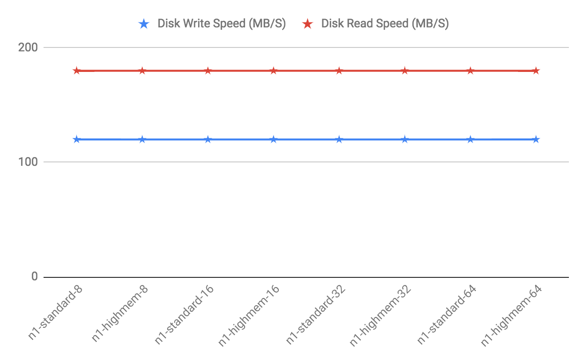
GCP Recommendations
Testing has revealed that while using the same number of vCPUs, a cluster using a large instance type like n1-highmem-64 (64 vCPUs) will have lower performance than a cluster using more of the smaller instance types like n1-highmem-8 (8 vCPUs). In general, use 8x more nodes in GCP than you would in another environment like AWS while using the 8 vCPU instance types.
The HighMem instance type is slightly faster for higher concurrency. Furthermore, SSD disks are slightly faster also but come at a cost.
Master and Segment Instances
| Instance Type | Memory | vCPUs | Data Disks |
|---|---|---|---|
| n1-standard-8 | 30 | 8 | 1 |
| n1-highmem-8 | 52 | 8 | 1 |
Azure
Note On the Azure platform, in addition to bandwidth, the number of network connections present on a VM at any given moment can affect the VM’s network performance. The Azure networking stack maintains the state for each direction of a TCP/UDP connection in a data structures called a flow. A typical TCP/UDP connection will have 2 flows created: one for the inbound direction and another for the outbound direction. The number of network flows on Azure is limited to an upper bound. See Virtual machine network bandwidth in the Azure documentation for more details. In practice this can present scalability challenges for workloads based on the number of concurrent queries, and on the complexity of those queries. Always test your workload on Azure to validate that you are within the Azure limits, and be advised that if your workload increases you may hit Azure flow count boundaries at which point your workload may fail. Synx Data Labs recommends using the UDP interconnect, and not the TCP interconnect, when using Azure. A connection pooler and resource group settings can also be used to help keep flow counts at a lower level.
Virtual Machine Type
Each VM type has limits on disk throughput so picking a VM that doesn’t have a limit that is too low is essential. Most of Azure is designed for OLTP or Application workloads, which limits the choices for databases like SynxDB where throughput is more important. Disk type also plays a part in the throughput cap, so that needs to be considered too.
Compute
Most instance types in Azure have hyperthreading enabled, which means 1 vCPU equates to 2 cores. However, not all instance types have this feature, so for these others, 1 vCPU equates to 1 core.
The High Performance Compute (HPC) instance types have the fastest cores in Azure.
Memory
In general, the larger the virtual machine type, the more memory the VM will have.
Network
The Accelerated Networking option offloads CPU cycles for networking to “FPGA-based SmartNICs”. Virtual machine types either support this or do not, but most do support it. Testing of SynxDB hasn’t shown much difference and this is probably because of Azure’s preference for TCP over UDP. Despite this, UDPIFC interconnect is the ideal protocol to use in Azure.
There is an undocumented process in Azure that periodically runs on the host machines on UDP port 65330. When a query runs using UDP port 65330 and this undocumented process runs, the query will fail after one hour with an interconnect timeout error. This is fixed by reserving port 65330 so that SynxDB doesn’t use it.
Storage
Storage in Azure is either Premium (SSD) or Regular Storage (HDD). The available sizes are the same and max out at 4TB. Instance types either do or do not support Premium but, interestingly, the instance types that do support Premium storage, have a lower throughput limit. For example:
- Standard_E32s_v3 has a limit of 768 MB/s.
- Standard_E32_v3 was tested with
gpcheckperfto have 1424 write and 1557 read MB/s performance.
To get the maximum throughput from a VM in Azure, you have to use multiple disks. For larger instance types, you have to use upwards of 32 disks to reach the limit of a VM. Unfortunately, the memory and CPU constraints on these machines means that you have to run fewer segments than you have disks, so you have to use software RAID to utilize all of these disks. Performance takes a hit with software RAID, too, so you have to try multiple configurations to optimize.
The size of the disk also impacts performance, but not by much.
Software RAID not only is a little bit slower, but it also requires umount to take a snapshot. This greatly lengthens the time it takes to take a snapshot backup.
Disks use the same network as the VMs so you start running into the Azure limits in bigger clusters when using big virtual machines with 32 disks on each one. The overall throughput drops as you hit this limit and is most noticeable during concurrency testing.
Azure Recommendations
The best instance type to use in Azure is “Standard_H8” which is one of the High Performance Compute instance types. This instance series is the only one utilizing InfiniBand, but this does not include IP traffic. Because this instance type is n0t available in all regions, the “Standard_D13_v2” is also available.
Master
| Instance Type | Memory | vCPUs | Data Disks |
|---|---|---|---|
| D13_v2 | 56 | 8 | 1 |
| H8 | 56 | 8 | 1 |
Segments
| Instance Type | Memory | vCPUs | Data Disks |
|---|---|---|---|
| D13_v2 | 56 | 8 | 2 |
| H8 | 56 | 8 | 2 |
Estimating Storage Capacity
To estimate how much data your SynxDB system can accommodate, use these measurements as guidelines. Also keep in mind that you may want to have extra space for landing backup files and data load files on each segment host.
Calculating Usable Disk Capacity
To calculate how much data a SynxDB system can hold, you have to calculate the usable disk capacity per segment host and then multiply that by the number of segment hosts in your SynxDB array. Start with the raw capacity of the physical disks on a segment host that are available for data storage (raw_capacity), which is:
disk_size * number_of_disks
Account for file system formatting overhead (roughly 10 percent) and the RAID level you are using. For example, if using RAID-10, the calculation would be:
(raw_capacity * 0.9) / 2 = formatted_disk_space
For optimal performance, do not completely fill your disks to capacity, but run at 70% or lower. So with this in mind, calculate the usable disk space as follows:
formatted_disk_space * 0.7 = usable_disk_space
Using only 70% of your disk space allows SynxDB to use the other 30% for temporary and transaction files on the same disks. If your host systems have a separate disk system that can be used for temporary and transaction files, you can specify a tablespace that SynxDB uses for the files. Moving the location of the files might improve performance depending on the performance of the disk system.
Once you have formatted RAID disk arrays and accounted for the maximum recommended capacity (usable_disk_space), you will need to calculate how much storage is actually available for user data (U). If using SynxDB mirrors for data redundancy, this would then double the size of your user data (2 * U). SynxDB also requires some space be reserved as a working area for active queries. The work space should be approximately one third the size of your user data (work space = U/3):
With mirrors: (2 * U) + U/3 = usable_disk_space
Without mirrors: U + U/3 = usable_disk_space
Guidelines for temporary file space and user data space assume a typical analytic workload. Highly concurrent workloads or workloads with queries that require very large amounts of temporary space can benefit from reserving a larger working area. Typically, overall system throughput can be increased while decreasing work area usage through proper workload management. Additionally, temporary space and user space can be isolated from each other by specifying that they reside on different tablespaces.
In the SynxDB Administrator Guide, see these topics:
- Managing Performance for information about workload management
- Creating and Managing Tablespaces for information about moving the location of temporary and transaction files
- Monitoring System State for information about monitoring SynxDB disk space usage
Calculating User Data Size
As with all databases, the size of your raw data will be slightly larger once it is loaded into the database. On average, raw data will be about 1.4 times larger on disk after it is loaded into the database, but could be smaller or larger depending on the data types you are using, table storage type, in-database compression, and so on.
-
Page Overhead - When your data is loaded into SynxDB, it is divided into pages of 32KB each. Each page has 20 bytes of page overhead.
-
Row Overhead - In a regular ‘heap’ storage table, each row of data has 24 bytes of row overhead. An ‘append-optimized’ storage table has only 4 bytes of row overhead.
-
Attribute Overhead - For the data values itself, the size associated with each attribute value is dependent upon the data type chosen. As a general rule, you want to use the smallest data type possible to store your data (assuming you know the possible values a column will have).
-
Indexes - In SynxDB, indexes are distributed across the segment hosts as is table data. The default index type in SynxDB is B-tree. Because index size depends on the number of unique values in the index and the data to be inserted, precalculating the exact size of an index is impossible. However, you can roughly estimate the size of an index using these formulas.
B-tree: unique_values * (data_type_size + 24 bytes) Bitmap: (unique_values * =number_of_rows * 1 bit * compression_ratio / 8) + (unique_values * 32)
Calculating Space Requirements for Metadata and Logs
On each segment host, you will also want to account for space for SynxDB log files and metadata:
-
System Metadata — For each SynxDB segment instance (primary or mirror) or master instance running on a host, estimate approximately 20 MB for the system catalogs and metadata.
-
Write Ahead Log — For each SynxDB segment (primary or mirror) or master instance running on a host, allocate space for the write ahead log (WAL). The WAL is divided into segment files of 64 MB each. At most, the number of WAL files will be:
2 * checkpoint_segments + 1You can use this to estimate space requirements for WAL. The default checkpoint_segments setting for a SynxDB instance is 8, meaning 1088 MB WAL space allocated for each segment or master instance on a host.
-
SynxDB Log Files — Each segment instance and the master instance generates database log files, which will grow over time. Sufficient space should be allocated for these log files, and some type of log rotation facility should be used to ensure that to log files do not grow too large.
Configuring Your Systems
Describes how to prepare your operating system environment for SynxDB software installation.
Perform the following tasks in order:
- Make sure your host systems meet the requirements described in Platform Requirements.
- Deactivate or configure SELinux.
- Deactivate or configure firewall software.
- Set the required operating system parameters.
- Synchronize system clocks.
- Create the gpadmin account.
Unless noted, these tasks should be performed for all hosts in your SynxDB array (master, standby master, and segment hosts).
The SynxDB host naming convention for the master host is mdw and for the standby master host is smdw.
The segment host naming convention is sdwN where sdw is a prefix and N is an integer. For example, segment host names would be sdw1, sdw2 and so on. NIC bonding is recommended for hosts with multiple interfaces, but when the interfaces are not bonded, the convention is to append a dash (-) and number to the host name. For example, sdw1-1 and sdw1-2 are the two interface names for host sdw1.
Important When data loss is not acceptable for a SynxDB cluster, SynxDB master and segment mirroring is recommended. If mirroring is not enabled then SynxDB stores only one copy of the data, so the underlying storage media provides the only guarantee for data availability and correctness in the event of a hardware failure.
The SynxDB on vSphere virtualized environment ensures the enforcement of anti-affinity rules required for SynxDB mirroring solutions and fully supports mirrorless deployments. Other virtualized or containerized deployment environments are generally not supported for production use unless both SynxDB master and segment mirroring are enabled.
Note For information about upgrading SynxDB from a previous version, see the SynxDB Release Notes for the release that you are installing.
Note Automating the configuration steps described in this topic and Installing the SynxDB Software with a system provisioning tool, such as Ansible, Chef, or Puppet, can save time and ensure a reliable and repeatable SynxDB installation.
Deactivate or Configure SELinux
For all SynxDB host systems, SELinux must either be Disabled or configured to allow unconfined access to SynxDB processes, directories, and the gpadmin user.
If you choose to deactivate SELinux:
-
As the root user, check the status of SELinux:
# sestatus SELinuxstatus: disabled -
If SELinux is not deactivated, deactivate it by editing the
/etc/selinux/configfile. As root, change the value of theSELINUXparameter in theconfigfile as follows:SELINUX=disabled -
If the System Security Services Daemon (SSSD) is installed on your systems, edit the SSSD configuration file and set the
selinux_providerparameter tononeto prevent SELinux-related SSH authentication denials that could occur even with SELinux deactivated. As root, edit/etc/sssd/sssd.confand add this parameter:selinux_provider=none -
Reboot the system to apply any changes that you made and verify that SELinux is deactivated.
If you choose to enable SELinux in Enforcing mode, then SynxDB processes and users can operate successfully in the default Unconfined context. If you require increased SELinux confinement for SynxDB processes and users, you must test your configuration to ensure that there are no functionality or performance impacts to SynxDB. See the SELinux User’s and Administrator’s Guide for detailed information about configuring SELinux and SELinux users.
Deactivate or Configure Firewall Software
You should also deactivate firewall software such as firewalld. If firewall software is not deactivated, you must instead configure your software to allow required communication between SynxDB hosts.
To deactivate firewalld:
-
check the status of
firewalldwith the command:# systemctl status firewalldIf
firewalldis deactivated, the command output is:* firewalld.service - firewalld - dynamic firewall daemon Loaded: loaded (/usr/lib/systemd/system/firewalld.service; disabled; vendor preset: enabled) Active: inactive (dead) -
If necessary, run these commands as root to deactivate
firewalld:# systemctl stop firewalld.service # systemctl deactivate firewalld.service
See the documentation for the firewall or your operating system for additional information.
Recommended OS Parameters Settings
SynxDB requires that certain Linux operating system (OS) parameters be set on all hosts in your SynxDB system (masters and segments).
In general, the following categories of system parameters need to be altered:
- Shared Memory - A SynxDB instance will not work unless the shared memory segment for your kernel is properly sized. Most default OS installations have the shared memory values set too low for SynxDB. On Linux systems, you must also deactivate the OOM (out of memory) killer. For information about SynxDB shared memory requirements, see the SynxDB server configuration parameter shared_buffers in the SynxDB Reference Guide.
- Network - On high-volume SynxDB systems, certain network-related tuning parameters must be set to optimize network connections made by the SynxDB interconnect.
- User Limits - User limits control the resources available to processes started by a user’s shell. SynxDB requires a higher limit on the allowed number of file descriptors that a single process can have open. The default settings may cause some SynxDB queries to fail because they will run out of file descriptors needed to process the query.
More specifically, you need to edit the following Linux configuration settings:
- The hosts File
- The sysctl.conf File
- System Resources Limits
- Core Dump
- XFS Mount Options
- Disk I/O Settings
- Read ahead values
- Disk I/O scheduler disk access
- Networking
- Transparent Huge Pages (THP)
- SSH Connection Threshold
The hosts File
Edit the /etc/hosts file and make sure that it includes the host names and all interface address names for every machine participating in your SynxDB system.
The sysctl.conf File
The sysctl.conf parameters listed in this topic are for performance, optimization, and consistency in a wide variety of environments. Change these settings according to your specific situation and setup.
Set the parameters in the /etc/sysctl.conf file and reload with sysctl -p:
# kernel.shmall = _PHYS_PAGES / 2 # See Shared Memory Pages
kernel.shmall = 197951838
# kernel.shmmax = kernel.shmall * PAGE_SIZE
kernel.shmmax = 810810728448
kernel.shmmni = 4096
vm.overcommit_memory = 2 # See Segment Host Memory
vm.overcommit_ratio = 95 # See Segment Host Memory
net.ipv4.ip_local_port_range = 10000 65535 # See Port Settings
kernel.sem = 250 2048000 200 8192
kernel.sysrq = 1
kernel.core_uses_pid = 1
kernel.msgmnb = 65536
kernel.msgmax = 65536
kernel.msgmni = 2048
net.ipv4.tcp_syncookies = 1
net.ipv4.conf.default.accept_source_route = 0
net.ipv4.tcp_max_syn_backlog = 4096
net.ipv4.conf.all.arp_filter = 1
net.ipv4.ipfrag_high_thresh = 41943040
net.ipv4.ipfrag_low_thresh = 31457280
net.ipv4.ipfrag_time = 60
net.core.netdev_max_backlog = 10000
net.core.rmem_max = 2097152
net.core.wmem_max = 2097152
vm.swappiness = 10
vm.zone_reclaim_mode = 0
vm.dirty_expire_centisecs = 500
vm.dirty_writeback_centisecs = 100
vm.dirty_background_ratio = 0 # See System Memory
vm.dirty_ratio = 0
vm.dirty_background_bytes = 1610612736
vm.dirty_bytes = 4294967296
Shared Memory Pages
SynxDB uses shared memory to communicate between postgres processes that are part of the same postgres instance. kernel.shmall sets the total amount of shared memory, in pages, that can be used system wide. kernel.shmmax sets the maximum size of a single shared memory segment in bytes.
Set kernel.shmall and kernel.shmmax values based on your system’s physical memory and page size. In general, the value for both parameters should be one half of the system physical memory.
Use the operating system variables _PHYS_PAGES and PAGE_SIZE to set the parameters.
kernel.shmall = ( _PHYS_PAGES / 2)
kernel.shmmax = ( _PHYS_PAGES / 2) * PAGE_SIZE
To calculate the values for kernel.shmall and kernel.shmmax, run the following commands using the getconf command, which returns the value of an operating system variable.
$ echo $(expr $(getconf _PHYS_PAGES) / 2)
$ echo $(expr $(getconf _PHYS_PAGES) / 2 \* $(getconf PAGE_SIZE))
As best practice, we recommend you set the following values in the /etc/sysctl.conf file using calculated values. For example, a host system has 1583 GB of memory installed and returns these values: _PHYS_PAGES = 395903676 and PAGE_SIZE = 4096. These would be the kernel.shmall and kernel.shmmax values:
kernel.shmall = 197951838
kernel.shmmax = 810810728448
If the SynxDB master has a different shared memory configuration than the segment hosts, the _PHYS_PAGES and PAGE_SIZE values might differ, and the kernel.shmall and kernel.shmmax values on the master host will differ from those on the segment hosts.
Segment Host Memory
The vm.overcommit_memory Linux kernel parameter is used by the OS to determine how much memory can be allocated to processes. For SynxDB, this parameter should always be set to 2.
vm.overcommit_ratio is the percent of RAM that is used for application processes and the remainder is reserved for the operating system. The default is 50 on Red Hat Enterprise Linux.
For vm.overcommit_ratio tuning and calculation recommendations with resource group-based resource management or resource queue-based resource management, refer to Options for Configuring Segment Host Memory in the SynxDB Administrator Guide.
Port Settings
To avoid port conflicts between SynxDB and other applications during SynxDB initialization, make a note of the port range specified by the operating system parameter net.ipv4.ip_local_port_range. When initializing SynxDB using the gpinitsystem cluster configuration file, do not specify SynxDB ports in that range. For example, if net.ipv4.ip_local_port_range = 10000 65535, set the SynxDB base port numbers to these values.
PORT_BASE = 6000
MIRROR_PORT_BASE = 7000
For information about the gpinitsystem cluster configuration file, see Initializing a SynxDB System.
For Azure deployments with SynxDB avoid using port 65330; add the following line to sysctl.conf:
net.ipv4.ip_local_reserved_ports=65330
For additional requirements and recommendations for cloud deployments, see SynxDB Cloud Technical Recommendations.
IP Fragmentation Settings
When the SynxDB interconnect uses UDP (the default), the network interface card controls IP packet fragmentation and reassemblies.
If the UDP message size is larger than the size of the maximum transmission unit (MTU) of a network, the IP layer fragments the message. (Refer to Networking later in this topic for more information about MTU sizes for SynxDB.) The receiver must store the fragments in a buffer before it can reorganize and reassemble the message.
The following sysctl.conf operating system parameters control the reassembly process:
| OS Parameter | Description |
|---|---|
| net.ipv4.ipfrag_high_thresh | The maximum amount of memory used to reassemble IP fragments before the kernel starts to remove fragments to free up resources. The default value is 4194304 bytes (4MB). |
| net.ipv4.ipfrag_low_thresh | The minimum amount of memory used to reassemble IP fragments. The default value is 3145728 bytes (3MB). (Deprecated after kernel version 4.17.) |
| net.ipv4.ipfrag_time | The maximum amount of time (in seconds) to keep an IP fragment in memory. The default value is 30. |
The recommended settings for these parameters for SynxDB follow:
net.ipv4.ipfrag_high_thresh = 41943040
net.ipv4.ipfrag_low_thresh = 31457280
net.ipv4.ipfrag_time = 60
System Memory
For host systems with more than 64GB of memory, these settings are recommended:
vm.dirty_background_ratio = 0
vm.dirty_ratio = 0
vm.dirty_background_bytes = 1610612736 # 1.5GB
vm.dirty_bytes = 4294967296 # 4GB
For host systems with 64GB of memory or less, remove vm.dirty_background_bytes and vm.dirty_bytes and set the two ratio parameters to these values:
vm.dirty_background_ratio = 3
vm.dirty_ratio = 10
Increase vm.min_free_kbytes to ensure PF_MEMALLOC requests from network and storage drivers are easily satisfied. This is especially critical on systems with large amounts of system memory. The default value is often far too low on these systems. Use this awk command to set vm.min_free_kbytes to a recommended 3% of system physical memory:
awk 'BEGIN {OFMT = "%.0f";} /MemTotal/ {print "vm.min_free_kbytes =", $2 * .03;}'
/proc/meminfo >> /etc/sysctl.conf
Do not set vm.min_free_kbytes to higher than 5% of system memory as doing so might cause out of memory conditions.
System Resources Limits
Set the following parameters in the /etc/security/limits.conf file:
* soft nofile 524288
* hard nofile 524288
* soft nproc 131072
* hard nproc 131072
Parameter values in the /etc/security/limits.d/20-nproc.conf file override the values in the limits.conf file. Ensure that any parameters in the override file are set to the required value. The Linux module pam_limits sets user limits by reading the values from the limits.conf file and then from the override file. For information about PAM and user limits, see the documentation on PAM and pam_limits.
Run the ulimit -u command on each segment host to display the maximum number of processes that are available to each user. Validate that the return value is 131072.
Core Dump
Enable core file generation to a known location by adding the following line to /etc/sysctl.conf:
kernel.core_pattern=/var/core/core.%h.%t
Add the following line to /etc/security/limits.conf:
* soft core unlimited
To apply the changes to the live kernel, run the following command:
# sysctl -p
XFS Mount Options
XFS is the preferred data storage file system on Linux platforms. Use the mount command with the following recommended XFS mount options:
rw,nodev,noatime,nobarrier,inode64
See the mount manual page (man mount opens the man page) for more information about using this command.
The XFS options can also be set in the /etc/fstab file. This example entry from an fstab file specifies the XFS options.
/dev/data /data xfs nodev,noatime,inode64 0 0
Note You must have root permission to edit the
/etc/fstabfile.
Disk I/O Settings
-
Read-ahead value
Each disk device file should have a read-ahead (
blockdev) value of 16384. To verify the read-ahead value of a disk device:# sudo /sbin/blockdev --getra <devname>For example:
# sudo /sbin/blockdev --getra /dev/sdbTo set blockdev (read-ahead) on a device:
# sudo /sbin/blockdev --setra <bytes> <devname>For example:
# sudo /sbin/blockdev --setra 16384 /dev/sdbSee the manual page (man) for the
blockdevcommand for more information about using that command (man blockdevopens the man page).Note The
blockdev --setracommand is not persistent. You must ensure the read-ahead value is set whenever the system restarts. How to set the value will vary based on your system.One method to set the
blockdevvalue at system startup is by adding the/sbin/blockdev --setracommand in therc.localfile. For example, add this line to therc.localfile to set the read-ahead value for the disksdb./sbin/blockdev --setra 16384 /dev/sdbOn systems that use systemd, you must also set the execute permissions on the
rc.localfile to enable it to run at startup. For example, this command sets execute permissions on the file.# chmod +x /etc/rc.d/rc.localRestart the system to have the setting take effect.
-
Disk I/O scheduler
The Linux disk scheduler orders the I/O requests submitted to a storage device, controlling the way the kernel commits reads and writes to disk.
A typical Linux disk I/O scheduler supports multiple access policies. The optimal policy selection depends on the underlying storage infrastructure. The recommended scheduler policy settings for SynxDB systems for specific OSs and storage device types follow:
Storage Device Type Recommended Scheduler Policy Non-Volatile Memory Express (NVMe) noneSolid-State Drives (SSD) noneOther mqdeadlineTo specify a scheduler until the next system reboot, run the following:
# echo schedulername > /sys/block/<devname>/queue/schedulerFor example:
# echo deadline > /sys/block/sbd/queue/schedulerNote Using the
echocommand to set the disk I/O scheduler policy is not persistent; you must ensure that you run the command whenever the system reboots. How to run the command will vary based on your system.To specify the I/O scheduler at boot time on systems that use
grub2, use the system utilitygrubby. This command adds the parameter when run asroot:# grubby --update-kernel=ALL --args="elevator=deadline"After adding the parameter, reboot the system.
This
grubbycommand displays kernel parameter settings:# grubby --info=ALLRefer to your operating system documentation for more information about the
grubbyutility.For additional information about configuring the disk scheduler, refer to the Enterprise Linux documentation for EL 8 or EL 9.
Networking
The maximum transmission unit (MTU) of a network specifies the size (in bytes) of the largest data packet/frame accepted by a network-connected device. A jumbo frame is a frame that contains more than the standard MTU of 1500 bytes.
You may control the value of the MTU at various locations:
- The SynxDB gp_max_packet_size server configuration parameter. The default max packet size is 8192. This default assumes a jumbo frame MTU.
- The operating system MTU settings for network interfaces.
- The physical switch MTU settings.
- The virtual switch MTU setting when using vSphere.
These settings are connected, in that they should always be either the same, or close to the same, value, or otherwise in the order of SynxDB < Operating System < Virtual or Physical switch for MTU size.
9000 is a common supported setting for switches, and is the recommended OS and rack switch MTU setting for your SynxDB hosts.
Transparent Huge Pages (THP)
Deactivate Transparent Huge Pages (THP) as it degrades SynxDB performance. THP is enabled by default. On systems that use grub2, use the system utility grubby. This command adds the parameter when run as root:
# grubby --update-kernel=ALL --args="transparent_hugepage=never"
After adding the parameter, reboot the system.
This cat command checks the state of THP. The output indicates that THP is deactivated.
$ cat /sys/kernel/mm/*transparent_hugepage/enabled
always [never]
For more information about Transparent Huge Pages or the grubby utility, see your operating system documentation.
SSH Connection Threshold
Certain SynxDB management utilities including gpexpand, gpinitsystem, and gpaddmirrors, use secure shell (SSH) connections between systems to perform their tasks. In large SynxDB deployments, cloud deployments, or deployments with a large number of segments per host, these utilities may exceed the host’s maximum threshold for unauthenticated connections. When this occurs, you receive errors such as: ssh_exchange_identification: Connection closed by remote host.
To increase this connection threshold for your SynxDB system, update the SSH MaxStartups and MaxSessions configuration parameters in one of the /etc/ssh/sshd_config or /etc/sshd_config SSH daemon configuration files.
Note You must have root permission to edit these two files.
If you specify MaxStartups and MaxSessions using a single integer value, you identify the maximum number of concurrent unauthenticated connections (MaxStartups) and maximum number of open shell, login, or subsystem sessions permitted per network connection (MaxSessions). For example:
MaxStartups 200
MaxSessions 200
If you specify MaxStartups using the “start:rate:full” syntax, you enable random early connection drop by the SSH daemon. start identifies the maximum number of unauthenticated SSH connection attempts allowed. Once start number of unauthenticated connection attempts is reached, the SSH daemon refuses rate percent of subsequent connection attempts. full identifies the maximum number of unauthenticated connection attempts after which all attempts are refused. For example:
Max Startups 10:30:200
MaxSessions 200
Restart the SSH daemon after you update MaxStartups and MaxSessions. For example, run the following command as the root user:
# service sshd restart
For detailed information about SSH configuration options, refer to the SSH documentation for your Linux distribution.
Synchronizing System Clocks
You must use NTP (Network Time Protocol) to synchronize the system clocks on all hosts that comprise your SynxDB system. Accurate time keeping is essential to ensure reliable operations on the database and data integrity.
There are many different architectures you may choose from to implement NTP. We recommend you use one of the following:
- Configure master as the NTP primary source and the other hosts in the cluster connect to it.
- Configure an external NTP primary source and all hosts in the cluster connect to it.
Depending on your operating system version, the NTP protocol may be implemented by the ntpd daemon, the chronyd daemon, or other. Refer to your preferred NTP protocol documentation for more details.
Option 1: Configure System Clocks with the Coordinator as the Primary Source
-
On the master host, log in as root and edit your NTP daemon configuration file. Set the
serverparameter to point to your data center’s NTP time server. For example (if10.6.220.20was the IP address of your data center’s NTP server):server 10.6.220.20 -
On each segment host, log in as root and edit your NTP daemon configuration file. Set the first
serverparameter to point to the master host, and the second server parameter to point to the standby master host. For example:server mdw prefer server smdw -
On the standby master host, log in as root and edit the
/etc/ntp.conffile. Set the firstserverparameter to point to the primary master host, and the second server parameter to point to your data center’s NTP time server. For example:server mdw prefer server 10.6.220.20 -
Synchronize the system clocks on all SynxDB hosts as root. If you are using the
ntpddaemon:systemctl restart ntpIf you are using the
chronyddaemon:systemctl restart chronyd
Option 2: Configure System Clocks with an External Primary Source
-
On each host, including coordinator, standby coordinator, and segments, log in as root and edit your NTP daemon configuration file. Set the first
serverparameter to point to your data center’s NTP time server. For example (if10.6.220.20was the IP address of your data center’s NTP server):server 10.6.220.20 -
On the coordinator host, use your NTP daemon to synchronize the system clocks on all SynxDB hosts. For example, using gpssh: If you are using the
ntpddaemon:gpssh -f hostfile_gpssh_allhosts -v -e 'ntpd'If you are using the
chronyddaemon:gpssh -f hostfile_gpssh_allhosts -v -e 'chronyd'
Creating the SynxDB Administrative User
Create a dedicated operating system user account on each node to run and administer SynxDB. This user account is named gpadmin by convention.
Important You cannot run the SynxDB server as
root.
The gpadmin user must have permission to access the services and directories required to install and run SynxDB.
The gpadmin user on each SynxDB host must have an SSH key pair installed and be able to SSH from any host in the cluster to any other host in the cluster without entering a password or passphrase (called “passwordless SSH”). If you enable passwordless SSH from the master host to every other host in the cluster (“1-n passwordless SSH”), you can use the SynxDB gpssh-exkeys command-line utility later to enable passwordless SSH from every host to every other host (“n-n passwordless SSH”).
You can optionally give the gpadmin user sudo privilege, so that you can easily administer all hosts in the SynxDB cluster as gpadmin using the sudo, ssh/scp, and gpssh/gpscp commands.
The following steps show how to set up the gpadmin user on a host, set a password, create an SSH key pair, and (optionally) enable sudo capability. These steps must be performed as root on every SynxDB cluster host. (For a large SynxDB cluster you will want to automate these steps using your system provisioning tools.)
Note See Example Ansible Playbook for an example that shows how to automate the tasks of creating the
gpadminuser and installing the SynxDB software on all hosts in the cluster.
-
Create the
gpadmingroup and user.This example creates the
gpadmingroup, creates thegpadminuser as a system account with a home directory and as a member of thegpadmingroup, and creates a password for the user.# groupadd gpadmin # useradd gpadmin -r -m -g gpadmin # passwd gpadmin New password: <changeme> Retype new password: <changeme>Note You must have root permission to create the
gpadmingroup and user.Note Make sure the
gpadminuser has the same user id (uid) and group id (gid) numbers on each host to prevent problems with scripts or services that use them for identity or permissions. For example, backing up SynxDB databases to some networked filesy stems or storage appliances could fail if thegpadminuser has different uid or gid numbers on different segment hosts. When you create thegpadmingroup and user, you can use thegroupadd -goption to specify a gid number and theuseradd -uoption to specify the uid number. Use the commandid gpadminto see the uid and gid for thegpadminuser on the current host. -
Switch to the
gpadminuser and generate an SSH key pair for thegpadminuser.$ su gpadmin $ ssh-keygen -t rsa -b 4096 Generating public/private rsa key pair. Enter file in which to save the key (/home/gpadmin/.ssh/id_rsa): Created directory '/home/gpadmin/.ssh'. Enter passphrase (empty for no passphrase): Enter same passphrase again:At the passphrase prompts, press Enter so that SSH connections will not require entry of a passphrase.
-
Grant sudo access to the
gpadminuser. Runvisudoand uncomment the%wheelgroup entry.%wheel ALL=(ALL) NOPASSWD: ALLMake sure you uncomment the line that has the
NOPASSWDkeyword.Add the
gpadminuser to thewheelgroup with this command.# usermod -aG wheel gpadmin
Next Steps
Installing the SynxDB Software
Describes how to install the SynxDB software binaries on all of the hosts that will comprise your SynxDB system, how to enable passwordless SSH for the gpadmin user, and how to verify the installation.
Perform the following tasks in order:
Installing SynxDB
You must install SynxDB on each host machine of the SynxDB cluster.
Synx Data Labs distributes the SynxDB software via a repository that must be installed on each cluster host. This guide assumes that each host can access the Synx Data Labs repositories. If your environment restricts internet access, or if you prefer to host repositories within your infrastructure to ensure consistent package availability, contact Synx Data Labs to obtain a complete repository mirror for local hosting.
Perform the following steps on each host machine of your cluster:
Follow these steps to securely install SynxDB to your system:
-
Login to your Enterprise Linux 8 or 9 system as the
rootuser. -
Import the Synx Data Labs GPG key so you can use it to validate downloaded packages:
wget -nv https://synxdb-repo.s3.us-west-2.amazonaws.com/gpg/RPM-GPG-KEY-SYNXDB rpm --import RPM-GPG-KEY-SYNXDB -
Verify that you have imported the keys:
rpm -q gpg-pubkey --qf "%{NAME}-%{VERSION}-%{RELEASE} %{SUMMARY}\n" | grep SynxDBYou should see output similar to:
gpg-pubkey-df4bfefe-67975261 gpg(SynxDB Infrastructure <infrastructure@synxdata.com>) -
Download the SynxDB repository package:
wget -nv https://synxdb-repo.s3.us-west-2.amazonaws.com/repo-release/synxdb2-release-1-1.rpm -
Verify the package signature of the repository package you just downloaded.
rpm --checksig synxdb2-release-1-1.rpmEnsure that the command output shows that the signature is OK. For example:
synxdb2-release-1-1.rpm: digests signatures OK -
After verifying the package signature, install the SynxDB repository package. For Enterprise Linux 9:
dnf install -y synxdb2-release-1-1.rpmThe repository installation shows details of the installation process similar to:
Last metadata expiration check: 2:11:29 ago on Mon Mar 10 18:53:32 2025. Dependencies resolved. ========================================================================= Package Architecture Version Repository Size ========================================================================= Installing: synxdb-release noarch 1-1 @commandline 8.1 k Transaction Summary ========================================================================= Install 1 Package Total size: 8.1 k Installed size: 0 Downloading Packages: Running transaction check Transaction check succeeded. Running transaction test Transaction test succeeded. Running transaction Preparing : 1/1 Running scriptlet: synxdb2-release-1-1.noarch 1/1 Installing : synxdb2-release-1-1.noarch 1/1 Verifying : synxdb2-release-1-1.noarch 1/1 Installed: synxdb2-release-1-1.noarch Complete!Note: The
-yoption in thednf installcommand automatically confirms and proceeds with installing the software as well as dependent packages. If you prefer to confirm each dependency manually, omit the-yflag. -
After you have installed the repository package, install SynxDB with the command:
dnf install -y synxdbThe installation process installs all dependencies required for SynxDB 2 in addition to the SynxDB software.
-
Verify the installation with:
rpm -qi synxdbYou should see installation details similar to:
Name : synxdb Version : 2.27.2 Release : 1.el8 Architecture: x86_64 Install Date: Fri Mar 14 17:22:59 2025 Group : Applications/Databases Size : 1541443881 License : ASL 2.0 Signature : RSA/SHA256, Thu Mar 13 10:36:01 2025, Key ID b783878edf4bfefe Source RPM : synxdb-2.27.2-1.el8.src.rpm Build Date : Thu Mar 13 09:55:50 2025 Build Host : cdw Relocations : /usr/local/synxdb Vendor : Synx Data Labs, Inc. URL : https://synxdatalabs.com Summary : High-performance MPP database for enterprise analytics Description : SynxDB is a high-performance, enterprise-grade, massively parallel processing (MPP) database designed for advanced analytics on large-scale data sets. Derived from PostgreSQL and the last open-source version of Greenplum, SynxDB offers seamless compatibility, powerful analytical capabilities, and robust security features. Key Features: - Massively parallel processing for optimized query performance - Advanced analytics for complex data workloads - Seamless integration with ETL pipelines and BI tools - Broad compatibility with diverse data sources and formats - Enhanced security and operational reliability Disclaimer & Attribution: SynxDB is derived from the last open-source version of Greenplum, originally developed by Pivotal Software, Inc., and maintained under Broadcom Inc.'s stewardship. Greenplum® is a registered trademark of Broadcom Inc. Synx Data Labs, Inc. and SynxDB are not affiliated with, endorsed by, or sponsored by Broadcom Inc. References to Greenplum are provided for comparative, interoperability, and attribution purposes in compliance with open-source licensing requirements. For more information, visit the official SynxDB website at https://synxdatalabs.com.Also verify that the
/usr/local/synxdbdirectory points to the specific version of SynxDB that you downloaded:ls -ld /usr/local/synxdb*For version 2.27.2 the output is:
lrwxrwxrwx 1 root root 24 Feb 19 10:05 /usr/local/synxdb -> /usr/local/synxdb-2.27.2 drwxr-xr-x 10 root root 4096 Mar 10 21:07 /usr/local/synxdb-2.27.2 -
If you have not yet created the
gpadminadministrator user and group, execute these steps:# groupadd gpadmin # useradd gpadmin -r -m -g gpadmin # passwd gpadmin New password: <changeme> Retype new password: <changeme> -
Login as the
gpadminuser and set the SynxDB environment:su - gpadmin source /usr/local/synxdb/synxdb_path.sh -
Finally, verify that the following SynxDB executable paths and versions match the expected paths and versions for your installation:
# which postgres /usr/local/synxdb-2.27.2/bin/postgres # which psql /usr/local/synxdb-2.27.2/bin/psql # postgres --version postgres (SynxDB) 9.4.26 # postgres --gp-version postgres (SynxDB) 6.27.2+SynxDB_GA build 1 # psql --version psql (PostgreSQL) 9.4.26
Enabling Passwordless SSH
The gpadmin user on each SynxDB host must be able to SSH from any host in the cluster to any other host in the cluster without entering a password or passphrase (called “passwordless SSH”). If you enable passwordless SSH from the master host to every other host in the cluster (“1-n passwordless SSH”), you can use the SynxDB gpssh-exkeys command-line utility to enable passwordless SSH from every host to every other host (“n-n passwordless SSH”).
-
Log in to the master host as the
gpadminuser. -
Source the
pathfile in the SynxDB installation directory.$ source /usr/local/synxdb/synxdb_path.shNote Add the above
sourcecommand to thegpadminuser’s.bashrcor other shell startup file so that the SynxDB path and environment variables are set whenever you log in asgpadmin. -
Use the
ssh-copy-idcommand to add thegpadminuser’s public key to theauthorized_hostsSSH file on every other host in the cluster.$ ssh-copy-id smdw $ ssh-copy-id sdw1 $ ssh-copy-id sdw2 $ ssh-copy-id sdw3 . . .This enables 1-n passwordless SSH. You will be prompted to enter the
gpadminuser’s password for each host. If you have thesshpasscommand on your system, you can use a command like the following to avoid the prompt.$ SSHPASS=<password> sshpass -e ssh-copy-id smdw -
In the
gpadminhome directory, create a file namedhostfile_exkeysthat has the machine configured host names and host addresses (interface names) for each host in your SynxDB system (master, standby master, and segment hosts). Make sure there are no blank lines or extra spaces. Check the/etc/hostsfile on your systems for the correct host names to use for your environment. For example, if you have a master, standby master, and three segment hosts with two unbonded network interfaces per host, your file would look something like this:mdw mdw-1 mdw-2 smdw smdw-1 smdw-2 sdw1 sdw1-1 sdw1-2 sdw2 sdw2-1 sdw2-2 sdw3 sdw3-1 sdw3-2 -
Run the
gpssh-exkeysutility with yourhostfile_exkeysfile to enable n-n passwordless SSH for thegpadminuser.$ gpssh-exkeys -f hostfile_exkeys
Confirming Your Installation
To make sure the SynxDB software was installed and configured correctly, run the following confirmation steps from your SynxDB master host. If necessary, correct any problems before continuing on to the next task.
-
Log in to the master host as
gpadmin:$ su - gpadmin -
Use the
gpsshutility to see if you can log in to all hosts without a password prompt, and to confirm that the SynxDB software was installed on all hosts. Use thehostfile_exkeysfile you used to set up passwordless SSH. For example:$ gpssh -f hostfile_exkeys -e 'ls -l /usr/local/synxdb-<version>'If the installation was successful, you should be able to log in to all hosts without a password prompt. All hosts should show that they have the same contents in their installation directories, and that the directories are owned by the
gpadminuser.If you are prompted for a password, run the following command to redo the ssh key exchange:
$ gpssh-exkeys -f hostfile_exkeys
About Your SynxDB Installation
synxdb_path.sh— This file contains the environment variables for SynxDB. See Setting SynxDB Environment Variables.- bin — This directory contains the SynxDB management utilities. This directory also contains the PostgreSQL client and server programs, most of which are also used in SynxDB.
- docs/cli_help — This directory contains help files for SynxDB command-line utilities.
- docs/cli_help/gpconfigs — This directory contains sample
gpinitsystemconfiguration files and host files that can be modified and used when installing and initializing a SynxDB system. - ext — Bundled programs (such as Python) used by some SynxDB utilities.
- include — The C header files for SynxDB.
- lib — SynxDB and PostgreSQL library files.
- sbin — Supporting/Internal scripts and programs.
- share — Shared files for SynxDB.
Next Steps
Creating the Data Storage Areas
Describes how to create the directory locations where SynxDB data is stored for each master, standby, and segment instance.
Creating Data Storage Areas on the Master and Standby Master Hosts
A data storage area is required on the SynxDB master and standby master hosts to store SynxDB system data such as catalog data and other system metadata.
To create the data directory location on the master
The data directory location on the master is different than those on the segments. The master does not store any user data, only the system catalog tables and system metadata are stored on the master instance, therefore you do not need to designate as much storage space as on the segments.
-
Create or choose a directory that will serve as your master data storage area. This directory should have sufficient disk space for your data and be owned by the
gpadminuser and group. For example, run the following commands asroot:# mkdir -p /data/master -
Change ownership of this directory to the
gpadminuser. For example:# chown gpadmin:gpadmin /data/master -
Using gpssh, create the master data directory location on your standby master as well. For example:
# source /usr/local/synxdb/synxdb_path.sh # gpssh -h smdw -e 'mkdir -p /data/master' # gpssh -h smdw -e 'chown gpadmin:gpadmin /data/master'
Creating Data Storage Areas on Segment Hosts
Data storage areas are required on the SynxDB segment hosts for primary segments. Separate storage areas are required for mirror segments.
To create the data directory locations on all segment hosts
-
On the master host, log in as
root:# su -
Create a file called
hostfile_gpssh_segonly. This file should have only one machine configured host name for each segment host. For example, if you have three segment hosts:sdw1 sdw2 sdw3 -
Using gpssh, create the primary and mirror data directory locations on all segment hosts at once using the
hostfile_gpssh_segonlyfile you just created. For example:# source /usr/local/synxdb/synxdb_path.sh # gpssh -f hostfile_gpssh_segonly -e 'mkdir -p /data/primary' # gpssh -f hostfile_gpssh_segonly -e 'mkdir -p /data/mirror' # gpssh -f hostfile_gpssh_segonly -e 'chown -R gpadmin /data/*'
Next Steps
Validating Your Systems
Validate your hardware and network performance.
SynxDB provides a management utility called gpcheckperf, which can be used to identify hardware and system-level issues on the machines in your SynxDB array. gpcheckperf starts a session on the specified hosts and runs the following performance tests:
- Network Performance (
gpnetbench*) - Disk I/O Performance (
ddtest) - Memory Bandwidth (
streamtest)
Before using gpcheckperf, you must have a trusted host setup between the hosts involved in the performance test. You can use the utility gpssh-exkeys to update the known host files and exchange public keys between hosts if you have not done so already. Note that gpcheckperf calls to gpssh and gpscp, so these SynxDB utilities must be in your $PATH.
Validating Network Performance
To test network performance, run gpcheckperf with one of the network test run options: parallel pair test (-r N), serial pair test (-r n), or full matrix test (-r M). The utility runs a network benchmark program that transfers a 5 second stream of data from the current host to each remote host included in the test. By default, the data is transferred in parallel to each remote host and the minimum, maximum, average and median network transfer rates are reported in megabytes (MB) per second. If the summary transfer rate is slower than expected (less than 100 MB/s), you can run the network test serially using the -r n option to obtain per-host results. To run a full-matrix bandwidth test, you can specify -r M which will cause every host to send and receive data from every other host specified. This test is best used to validate if the switch fabric can tolerate a full-matrix workload.
Most systems in a SynxDB array are configured with multiple network interface cards (NICs), each NIC on its own subnet. When testing network performance, it is important to test each subnet individually. For example, considering the following network configuration of two NICs per host:
| SynxDB Host | Subnet1 NICs | Subnet2 NICs |
|---|---|---|
| Segment 1 | sdw1-1 | sdw1-2 |
| Segment 2 | sdw2-1 | sdw2-2 |
| Segment 3 | sdw3-1 | sdw3-2 |
You would create four distinct host files for use with the gpcheckperf network test:
| hostfile_gpchecknet_ic1 | hostfile_gpchecknet_ic2 |
|---|---|
| sdw1-1 | sdw1-2 |
| sdw2-1 | sdw2-2 |
| sdw3-1 | sdw3-2 |
You would then run gpcheckperf once per subnet. For example (if testing an even number of hosts, run in parallel pairs test mode):
$ gpcheckperf -f hostfile_gpchecknet_ic1 -r N -d /tmp > subnet1.out
$ gpcheckperf -f hostfile_gpchecknet_ic2 -r N -d /tmp > subnet2.out
If you have an odd number of hosts to test, you can run in serial test mode (-r n).
Validating Disk I/O and Memory Bandwidth
To test disk and memory bandwidth performance, run gpcheckperf with the disk and stream test run options (-r ds). The disk test uses the dd command (a standard UNIX utility) to test the sequential throughput performance of a logical disk or file system. The memory test uses the STREAM benchmark program to measure sustainable memory bandwidth. Results are reported in MB per second (MB/s).
To run the disk and stream tests
-
Log in on the master host as the
gpadminuser. -
Source the
synxdb_path.shpath file from your SynxDB installation. For example:$ source /usr/local/synxdb/synxdb_path.sh -
Create a host file named
hostfile_gpcheckperfthat has one host name per segment host. Do not include the master host. For example:sdw1 sdw2 sdw3 sdw4 -
Run the
gpcheckperfutility using thehostfile_gpcheckperffile you just created. Use the-doption to specify the file systems you want to test on each host (you must have write access to these directories). You will want to test all primary and mirror segment data directory locations. For example:$ gpcheckperf -f hostfile_gpcheckperf -r ds -D \ -d /data1/primary -d /data2/primary \ -d /data1/mirror -d /data2/mirror -
The utility may take a while to perform the tests as it is copying very large files between the hosts. When it is finished you will see the summary results for the Disk Write, Disk Read, and Stream tests.
Initializing a SynxDB System
Describes how to initialize a SynxDB database system.
The instructions in this chapter assume you have already prepared your hosts as described in Configuring Your Systems and installed the SynxDB software on all of the hosts in the system according to the instructions in Installing the SynxDB Software.
This chapter contains the following topics:
Overview
Because SynxDB is distributed, the process for initializing a SynxDB management system (DBMS) involves initializing several individual PostgreSQL database instances (called segment instances in SynxDB).
Each database instance (the master and all segments) must be initialized across all of the hosts in the system in such a way that they can all work together as a unified DBMS. SynxDB provides its own version of initdb called gpinitsystem, which takes care of initializing the database on the master and on each segment instance, and starting each instance in the correct order.
After the SynxDB database system has been initialized and started, you can then create and manage databases as you would in a regular PostgreSQL DBMS by connecting to the SynxDB master.
Initializing SynxDB
These are the high-level tasks for initializing SynxDB:
- Make sure you have completed all of the installation tasks described in Configuring Your Systems and Installing the SynxDB Software.
- Create a host file that contains the host addresses of your segments. See Creating the Initialization Host File.
- Create your SynxDB system configuration file. See Creating the SynxDB Configuration File.
- By default, SynxDB will be initialized using the locale of the master host system. Make sure this is the correct locale you want to use, as some locale options cannot be changed after initialization. See Configuring Timezone and Localization Settings for more information.
- Run the SynxDB initialization utility on the master host. See Running the Initialization Utility.
- Set the SynxDB timezone. See Setting the SynxDB Timezone.
- Set environment variables for the SynxDB user. See Setting SynxDB Environment Variables.
When performing the following initialization tasks, you must be logged into the master host as the gpadmin user, and to run SynxDB utilities, you must source the synxdb_path.sh file to set SynxDB environment variables. For example, if you are logged into the master, run these commands.
$ su - gpadmin
$ source /usr/local/synxdb/synxdb_path.sh
Creating the Initialization Host File
The gpinitsystem utility requires a host file that contains the list of addresses for each segment host. The initialization utility determines the number of segment instances per host by the number host addresses listed per host times the number of data directory locations specified in the gpinitsystem_config file.
This file should only contain segment host addresses (not the master or standby master). For segment machines with multiple, unbonded network interfaces, this file should list the host address names for each interface — one per line.
Note The SynxDB segment host naming convention is sdwN where sdw is a prefix and N is an integer. For example,
sdw2and so on. If hosts have multiple unbonded NICs, the convention is to append a dash (-) and number to the host name. For example,sdw1-1andsdw1-2are the two interface names for hostsdw1. However, NIC bonding is recommended to create a load-balanced, fault-tolerant network.
To create the initialization host file
-
Create a file named
hostfile_gpinitsystem. In this file add the host address name(s) of your segment host interfaces, one name per line, no extra lines or spaces. For example, if you have four segment hosts with two unbonded network interfaces each:sdw1-1 sdw1-2 sdw2-1 sdw2-2 sdw3-1 sdw3-2 sdw4-1 sdw4-2 -
Save and close the file.
Note If you are not sure of the host names and/or interface address names used by your machines, look in the
/etc/hostsfile.
Creating the SynxDB Configuration File
Your SynxDB configuration file tells the gpinitsystem utility how you want to configure your SynxDB system. An example configuration file can be found in $GPHOME/docs/cli_help/gpconfigs/gpinitsystem_config.
To create a gpinitsystem_config file
-
Make a copy of the
gpinitsystem_configfile to use as a starting point. For example:$ cp $GPHOME/docs/cli_help/gpconfigs/gpinitsystem_config \ /home/gpadmin/gpconfigs/gpinitsystem_config -
Open the file you just copied in a text editor.
Set all of the required parameters according to your environment. See gpinitsystem for more information. A SynxDB system must contain a master instance and at least two segment instances (even if setting up a single node system).
The
DATA_DIRECTORYparameter is what determines how many segments per host will be created. If your segment hosts have multiple network interfaces, and you used their interface address names in your host file, the number of segments will be evenly spread over the number of available interfaces.To specify
PORT_BASE, review the port range specified in thenet.ipv4.ip_local_port_rangeparameter in the/etc/sysctl.conffile. See Recommended OS Parameters Settings.Here is an example of the required parameters in the
gpinitsystem_configfile:SEG_PREFIX=gpseg PORT_BASE=6000 declare -a DATA_DIRECTORY=(/data1/primary /data1/primary /data1/primary /data2/primary /data2/primary /data2/primary) MASTER_HOSTNAME=mdw MASTER_DIRECTORY=/data/master MASTER_PORT=5432 TRUSTED SHELL=ssh CHECK_POINT_SEGMENTS=8 ENCODING=UNICODE -
(Optional) If you want to deploy mirror segments, uncomment and set the mirroring parameters according to your environment. To specify
MIRROR_PORT_BASE, review the port range specified under thenet.ipv4.ip_local_port_rangeparameter in the/etc/sysctl.conffile. Here is an example of the optional mirror parameters in thegpinitsystem_configfile:MIRROR_PORT_BASE=7000 declare -a MIRROR_DATA_DIRECTORY=(/data1/mirror /data1/mirror /data1/mirror /data2/mirror /data2/mirror /data2/mirror)Note You can initialize your SynxDB system with primary segments only and deploy mirrors later using the gpaddmirrors utility.
-
Save and close the file.
Running the Initialization Utility
The gpinitsystem utility will create a SynxDB system using the values defined in the configuration file.
These steps assume you are logged in as the gpadmin user and have sourced the synxdb_path.sh file to set SynxDB environment variables.
To run the initialization utility
-
Run the following command referencing the path and file name of your initialization configuration file (
gpinitsystem_config) and host file (hostfile_gpinitsystem). For example:$ cd ~ $ gpinitsystem -c gpconfigs/gpinitsystem_config -h gpconfigs/hostfile_gpinitsystemFor a fully redundant system (with a standby master and a spread mirror configuration) include the
-sand--mirror-mode=spreadoptions. For example:$ gpinitsystem -c gpconfigs/gpinitsystem_config -h gpconfigs/hostfile_gpinitsystem \ -s <standby_master_hostname> --mirror-mode=spreadDuring a new cluster creation, you may use the
-O output\_configuration\_fileoption to save the cluster configuration details in a file. For example:$ gpinitsystem -c gpconfigs/gpinitsystem_config -O gpconfigs/config_templateThis output file can be edited and used at a later stage as the input file of the
-Ioption, to create a new cluster or to recover from a backup. See gpinitsystem for further details.Note Calling
gpinitsystemwith the-Ooption does not initialize the SynxDB system; it merely generates and saves a file with cluster configuration details. -
The utility will verify your setup information and make sure it can connect to each host and access the data directories specified in your configuration. If all of the pre-checks are successful, the utility will prompt you to confirm your configuration. For example:
=> Continue with SynxDB creation? Yy/Nn -
Press
yto start the initialization. -
The utility will then begin setup and initialization of the master instance and each segment instance in the system. Each segment instance is set up in parallel. Depending on the number of segments, this process can take a while.
-
At the end of a successful setup, the utility will start your SynxDB system. You should see:
=> SynxDB instance successfully created.
Troubleshooting Initialization Problems
If the utility encounters any errors while setting up an instance, the entire process will fail, and could possibly leave you with a partially created system. Refer to the error messages and logs to determine the cause of the failure and where in the process the failure occurred. Log files are created in ~/gpAdminLogs.
Depending on when the error occurred in the process, you may need to clean up and then try the gpinitsystem utility again. For example, if some segment instances were created and some failed, you may need to stop postgres processes and remove any utility-created data directories from your data storage area(s). A backout script is created to help with this cleanup if necessary.
Using the Backout Script
If the gpinitsystem utility fails, it will create the following backout script if it has left your system in a partially installed state:
~/gpAdminLogs/backout_gpinitsystem_<user>_<timestamp>
You can use this script to clean up a partially created SynxDB system. This backout script will remove any utility-created data directories, postgres processes, and log files. After correcting the error that caused gpinitsystem to fail and running the backout script, you should be ready to retry initializing your SynxDB array.
The following example shows how to run the backout script:
$ bash ~/gpAdminLogs/backout_gpinitsystem_gpadmin_20071031_121053
Setting the SynxDB Timezone
As a best practice, configure SynxDB and the host systems to use a known, supported timezone. SynxDB uses a timezone from a set of internally stored PostgreSQL timezones. Setting the SynxDB timezone prevents SynxDB from selecting a timezone each time the cluster is restarted and sets the timezone for the SynxDB master and segment instances.
Use the gpconfig utility to show and set the SynxDB timezone. For example, these commands show the SynxDB timezone and set the timezone to US/Pacific.
$ gpconfig -s TimeZone
$ gpconfig -c TimeZone -v 'US/Pacific'
You must restart SynxDB after changing the timezone. The command gpstop -ra restarts SynxDB. The catalog view pg_timezone_names provides SynxDB timezone information.
For more information about the SynxDB timezone, see Configuring Timezone and Localization Settings.
Setting SynxDB Environment Variables
You must set environment variables in the SynxDB user (gpadmin) environment that runs SynxDB on the SynxDB master and standby master hosts. A synxdb_path.sh file is provided in the SynxDB installation directory with environment variable settings for SynxDB.
The SynxDB management utilities also require that the MASTER_DATA_DIRECTORY environment variable be set. This should point to the directory created by the gpinitsystem utility in the master data directory location.
Note The
synxdb_path.shscript changes the operating environment in order to support running the SynxDB-specific utilities. These same changes to the environment can negatively affect the operation of other system-level utilities, such aspsoryum. Use separate accounts for performing system administration and database administration, instead of attempting to perform both functions asgpadmin.
These steps ensure that the environment variables are set for the gpadmin user after a system reboot.
To set up the gpadmin environment for SynxDB
-
Open the
gpadminprofile file (such as.bashrc) in a text editor. For example:$ vi ~/.bashrc -
Add lines to this file to source the
synxdb_path.shfile and set theMASTER_DATA_DIRECTORYenvironment variable. For example:source /usr/local/synxdb/synxdb_path.sh export MASTER_DATA_DIRECTORY=/data/master/gpseg-1 -
(Optional) You may also want to set some client session environment variables such as
PGPORT,PGUSERandPGDATABASEfor convenience. For example:export PGPORT=5432 export PGUSER=gpadmin export PGDATABASE=gpadmin -
(Optional) If you use RHEL 7 or CentOS 7, add the following line to the end of the
.bashrcfile to enable using thepscommand in thesynxdb_path.shenvironment:export LD_PRELOAD=/lib64/libz.so.1 ps -
Save and close the file.
-
After editing the profile file, source it to make the changes active. For example:
$ source ~/.bashrc -
If you have a standby master host, copy your environment file to the standby master as well. For example:
$ cd ~ $ scp .bashrc <standby_hostname>:`pwd`
Note The
.bashrcfile should not produce any output. If you wish to have a message display to users upon logging in, use the.bash_profilefile instead.
Next Steps
After your system is up and running, the next steps are:
Allowing Client Connections
After a SynxDB is first initialized it will only allow local connections to the database from the gpadmin role (or whatever system user ran gpinitsystem). If you would like other users or client machines to be able to connect to SynxDB, you must give them access. See the SynxDB Administrator Guide for more information.
Creating Databases and Loading Data
After verifying your installation, you may want to begin creating databases and loading data. See Defining Database Objects and Loading and Unloading Data in the SynxDB Administrator Guide for more information about creating databases, schemas, tables, and other database objects in SynxDB and loading your data.
Installing Optional Extensions
Information about installing optional SynxDB extensions and packages, such as the Procedural Language extensions and the Python and R Data Science Packages.
Procedural Language, Machine Learning, and Geospatial Extensions
Optional. Use the SynxDB package manager (gppkg) to install SynxDB extensions such as PL/Java, PL/R, PostGIS, and MADlib, along with their dependencies, across an entire cluster. The package manager also integrates with existing scripts so that any packages are automatically installed on any new hosts introduced into the system following cluster expansion or segment host recovery.
See gppkg for more information, including usage.
Extension packages can be downloaded from the SynxDB page on Synx Data Labs. The extension documentation in the SynxDB Reference Guide contains information about installing extension packages and using extensions.
- SynxDB PL/R Language Extension
- SynxDB PL/Java Language Extension
- SynxDB MADlib Extension for Analytics
- SynxDB PostGIS Extension
Important If you intend to use an extension package with SynxDB 2 you must install and use a SynxDB extension package (gppkg files and contrib modules) that is built for SynxDB 2. Any custom modules that were used with earlier versions must be rebuilt for use with SynxDB 2.
Data Science Package for Python
SynxDB provides a collection of data science-related Python modules that can be used with the SynxDB PL/Python language. You can download these modules in .gppkg format from Synx Data Labs. Separate modules are provided for Python 2.7 and Python 3.9 development on RHEL7, RHEL8, and Ubuntu platforms.
This section contains the following information:
- Data Science Package for Python 2.7 Modules
- Data Science Package for Python 3.9 Modules
- Installing a Data Science Package for Python
- Uninstalling a Data Science Package for Python
For information about the SynxDB PL/Python Language, see SynxDB PL/Python Language Extension.
Data Science Package for Python 2.7 Modules
The following table lists the modules that are provided in the Data Science Package for Python 2.7.
Packages required for Deep Learning features of MADlib are now included. Note that it is not supported for RHEL 6.
| Module Name | Description/Used For |
|---|---|
| atomicwrites | Atomic file writes |
| attrs | Declarative approach for defining class attributes |
| Autograd | Gradient-based optimization |
| backports.functools-lru-cache | Backports functools.lru_cache from Python 3.3 |
| Beautiful Soup | Navigating HTML and XML |
| Blis | Blis linear algebra routines |
| Boto | Amazon Web Services library |
| Boto3 | The AWS SDK |
| botocore | Low-level, data-driven core of boto3 |
| Bottleneck | Fast NumPy array functions |
| Bz2file | Read and write bzip2-compressed files |
| Certifi | Provides Mozilla CA bundle |
| Chardet | Universal encoding detector for Python 2 and 3 |
| ConfigParser | Updated configparser module |
| contextlib2 | Backports and enhancements for the contextlib module |
| Cycler | Composable style cycles |
| cymem | Manage calls to calloc/free through Cython |
| Docutils | Python documentation utilities |
| enum34 | Backport of Python 3.4 Enum |
| Funcsigs | Python function signatures from PEP362 |
| functools32 | Backport of the functools module from Python 3.2.3 |
| funcy | Functional tools focused on practicality |
| future | Compatibility layer between Python 2 and Python 3 |
| futures | Backport of the concurrent.futures package from Python 3 |
| Gensim | Topic modeling and document indexing |
| h5py | Read and write HDF5 files |
| idna | Internationalized Domain Names in Applications (IDNA) |
| importlib-metadata | Read metadata from Python packages |
| Jinja2 | Stand-alone template engine |
| JMESPath | JSON Matching Expressions |
| Joblib | Python functions as pipeline jobs |
| jsonschema | JSON Schema validation |
| Keras (RHEL/CentOS 7 only) | Deep learning |
| Keras Applications | Reference implementations of popular deep learning models |
| Keras Preprocessing | Easy data preprocessing and data augmentation for deep learning models |
| kiwisolver | A fast implementation of the Cassowary constraint solver |
| Lifelines | Survival analysis |
| lxml | XML and HTML processing |
| MarkupSafe | Safely add untrusted strings to HTML/XML markup |
| Matplotlib | Python plotting package |
| mock | Rolling backport of unittest.mock |
| more-itertools | More routines for operating on iterables, beyond itertools |
| MurmurHash | Cython bindings for MurmurHash |
| NLTK | Natural language toolkit |
| NumExpr | Fast numerical expression evaluator for NumPy |
| NumPy | Scientific computing |
| packaging | Core utilities for Python packages |
| Pandas | Data analysis |
| pathlib, pathlib2 | Object-oriented filesystem paths |
| patsy | Package for describing statistical models and for building design matrices |
| Pattern-en | Part-of-speech tagging |
| pip | Tool for installing Python packages |
| plac | Command line arguments parser |
| pluggy | Plugin and hook calling mechanisms |
| preshed | Cython hash table that trusts the keys are pre-hashed |
| protobuf | Protocol buffers |
| py | Cross-python path, ini-parsing, io, code, log facilities |
| pyLDAvis | Interactive topic model visualization |
| PyMC3 | Statistical modeling and probabilistic machine learning |
| pyparsing | Python parsing |
| pytest | Testing framework |
| python-dateutil | Extensions to the standard Python datetime module |
| pytz | World timezone definitions, modern and historical |
| PyXB-X (Python3 only) | To generate Python code for classes that correspond to data structures defined by XMLSchema |
| PyYAML | YAML parser and emitter |
| regex | Alternative regular expression module, to replace re |
| requests | HTTP library |
| s3transfer | Amazon S3 transfer manager |
| scandir | Directory iteration function |
| scikit-learn | Machine learning data mining and analysis |
| SciPy | Scientific computing |
| setuptools | Download, build, install, upgrade, and uninstall Python packages |
| six | Python 2 and 3 compatibility library |
| smart-open | Utilities for streaming large files (S3, HDFS, gzip, bz2, and so forth) |
| spaCy | Large scale natural language processing |
| srsly | Modern high-performance serialization utilities for Python |
| StatsModels | Statistical modeling |
| subprocess32 | Backport of the subprocess module from Python 3 |
| Tensorflow (RHEL/CentOS 7 only) | Numerical computation using data flow graphs |
| Theano | Optimizing compiler for evaluating mathematical expressions on CPUs and GPUs |
| thinc | Practical Machine Learning for NLP |
| tqdm | Fast, extensible progress meter |
| urllib3 | HTTP library with thread-safe connection pooling, file post, and more |
| wasabi | Lightweight console printing and formatting toolkit |
| wcwidth | Measures number of Terminal column cells of wide-character codes |
| Werkzeug | Comprehensive WSGI web application library |
| wheel | A built-package format for Python |
| XGBoost | Gradient boosting, classifying, ranking |
| zipp | Backport of pathlib-compatible object wrapper for zip files |
Data Science Package for Python 3.9 Modules
The following table lists the modules that are provided in the Data Science Package for Python 3.9.
| Module Name | Description/Used For |
|---|---|
| absl-py | Abseil Python Common Libraries |
| arviz | Exploratory analysis of Bayesian models |
| astor | Read/rewrite/write Python ASTs |
| astunparse | An AST unparser for Python |
| autograd | Efficiently computes derivatives of numpy code |
| autograd-gamma | autograd compatible approximations to the derivatives of the Gamma-family of functions |
| backports.csv | Backport of Python 3 csv module |
| beautifulsoup4 | Screen-scraping library |
| blis | The Blis BLAS-like linear algebra library, as a self-contained C-extension |
| cachetools | Extensible memoizing collections and decorators |
| catalogue | Super lightweight function registries for your library |
| certifi | Python package for providing Mozilla’s CA Bundle |
| cffi | Foreign Function Interface for Python calling C code |
| cftime | Time-handling functionality from netcdf4-python |
| charset-normalizer | The Real First Universal Charset Detector. Open, modern and actively maintained alternative to Chardet. |
| cheroot | Highly-optimized, pure-python HTTP server |
| CherryPy | Object-Oriented HTTP framework |
| click | Composable command line interface toolkit |
| convertdate | Converts between Gregorian dates and other calendar systems |
| cryptography | A set of functions useful in cryptography and linear algebra |
| cycler | Composable style cycles |
| cymem | Manage calls to calloc/free through Cython |
| Cython | The Cython compiler for writing C extensions for the Python language |
| deprecat | Python @deprecat decorator to deprecate old python classes, functions or methods |
| dill | serialize all of python |
| fastprogress | A nested progress with plotting options for fastai |
| feedparser | Universal feed parser, handles RSS 0.9x, RSS 1.0, RSS 2.0, CDF, Atom 0.3, and Atom 1.0 feeds |
| filelock | A platform independent file lock |
| flatbuffers | The FlatBuffers serialization format for Python |
| fonttools | Tools to manipulate font files |
| formulaic | An implementation of Wilkinson formulas |
| funcy | A fancy and practical functional tools |
| future | Clean single-source support for Python 3 and 2 |
| gast | Python AST that abstracts the underlying Python version |
| gensim | Python framework for fast Vector Space Modelling |
| gluonts | GluonTS is a Python toolkit for probabilistic time series modeling, built around MXNet |
| google-auth | Google Authentication Library |
| google-auth-oauthlib | Google Authentication Library |
| google-pasta | pasta is an AST-based Python refactoring library |
| graphviz | Simple Python interface for Graphviz |
| greenlet | Lightweight in-process concurrent programming |
| grpcio | HTTP/2-based RPC framework |
| h5py | Read and write HDF5 files from Python |
| hijri-converter | Accurate Hijri-Gregorian dates converter based on the Umm al-Qura calendar |
| holidays | Generate and work with holidays in Python |
| idna | Internationalized Domain Names in Applications (IDNA) |
| importlib-metadata | Read metadata from Python packages |
| interface-meta | Provides a convenient way to expose an extensible API with enforced method signatures and consistent documentation |
| jaraco.classes | Utility functions for Python class constructs |
| jaraco.collections | Collection objects similar to those in stdlib by jaraco |
| jaraco.context | Context managers by jaraco |
| jaraco.functools | Functools like those found in stdlib |
| jaraco.text | Module for text manipulation |
| Jinja2 | A very fast and expressive template engine |
| joblib | Lightweight pipelining with Python functions |
| keras | Deep learning for humans |
| Keras-Preprocessing | Easy data preprocessing and data augmentation for deep learning models |
| kiwisolver | A fast implementation of the Cassowary constraint solver |
| korean-lunar-calendar | Korean Lunar Calendar |
| langcodes | Tools for labeling human languages with IETF language tags |
| libclang | Clang Python Bindings, mirrored from the official LLVM repo |
| lifelines | Survival analysis in Python, including Kaplan Meier, Nelson Aalen and regression |
| llvmlite | lightweight wrapper around basic LLVM functionality |
| lxml | Powerful and Pythonic XML processing library combining libxml2/libxslt with the ElementTree API |
| Markdown | Python implementation of Markdown |
| MarkupSafe | Safely add untrusted strings to HTML/XML markup |
| matplotlib | Python plotting package |
| more-itertools | More routines for operating on iterables, beyond itertools |
| murmurhash | Cython bindings for MurmurHash |
| mxnet | An ultra-scalable deep learning framework |
| mysqlclient | Python interface to MySQL |
| netCDF4 | Provides an object-oriented python interface to the netCDF version 4 library |
| nltk | Natural language toolkit |
| numba | Compiling Python code using LLVM |
| numexpr | Fast numerical expression evaluator for NumPy |
| numpy | Scientific computing |
| oauthlib | A generic, spec-compliant, thorough implementation of the OAuth request-signing logic |
| opt-einsum | Optimizing numpys einsum function |
| packaging | Core utilities for Python packages |
| pandas | Data analysis |
| pathy | pathlib.Path subclasses for local and cloud bucket storage |
| patsy | Package for describing statistical models and for building design matrices |
| Pattern | Web mining module for Python |
| pdfminer.six | PDF parser and analyzer |
| Pillow | Python Imaging Library |
| pmdarima | Python’s forecast::auto.arima equivalent |
| portend | TCP port monitoring and discovery |
| preshed | Cython hash table that trusts the keys are pre-hashed |
| prophet | Automatic Forecasting Procedure |
| protobuf | Protocol buffers |
| psycopg2 | PostgreSQL database adapter for Python |
| psycopg2-binary | psycopg2 - Python-PostgreSQL Database Adapter |
| pyasn1 | ASN.1 types and codecs |
| pyasn1-modules | pyasn1-modules |
| pycparser | C parser in Python |
| pydantic | Data validation and settings management using python type hints |
| pyLDAvis | Interactive topic model visualization |
| pymc3 | Statistical modeling and probabilistic machine learning |
| PyMeeus | Python implementation of Jean Meeus astronomical routines |
| pyparsing | Python parsing |
| python-dateutil | Extensions to the standard Python datetime module |
| python-docx | Create and update Microsoft Word .docx files |
| PyTorch | Tensors and Dynamic neural networks in Python with strong GPU acceleration |
| pytz | World timezone definitions, modern and historical |
| regex | Alternative regular expression module, to replace re |
| requests | HTTP library |
| requests-oauthlib | OAuthlib authentication support for Requests |
| rsa | OAuthlib authentication support for Requests |
| scikit-learn | Machine learning data mining and analysis |
| scipy | Scientific computing |
| semver | Python helper for Semantic Versioning |
| sgmllib3k | Py3k port of sgmllib |
| six | Python 2 and 3 compatibility library |
| sklearn | A set of python modules for machine learning and data mining |
| smart-open | Utilities for streaming large files (S3, HDFS, gzip, bz2, and so forth) |
| soupsieve | A modern CSS selector implementation for Beautiful Soup |
| spacy | Large scale natural language processing |
| spacy-legacy | Legacy registered functions for spaCy backwards compatibility |
| spacy-loggers | Logging utilities for SpaCy |
| spectrum | Spectrum Analysis Tools |
| SQLAlchemy | Database Abstraction Library |
| srsly | Modern high-performance serialization utilities for Python |
| statsmodels | Statistical modeling |
| tempora | Objects and routines pertaining to date and time |
| tensorboard | TensorBoard lets you watch Tensors Flow |
| tensorboard-data-server | Fast data loading for TensorBoard |
| tensorboard-plugin-wit | What-If Tool TensorBoard plugin |
| tensorflow | Numerical computation using data flow graphs |
| tensorflow-estimator | What-If Tool TensorBoard plugin |
| tensorflow-io-gcs-filesystem | TensorFlow IO |
| termcolor | simple termcolor wrapper |
| Theano-PyMC | Theano-PyMC |
| thinc | Practical Machine Learning for NLP |
| threadpoolctl | Python helpers to limit the number of threads used in the threadpool-backed of common native libraries used for scientific computing and data science |
| toolz | List processing tools and functional utilities |
| tqdm | Fast, extensible progress meter |
| tslearn | A machine learning toolkit dedicated to time-series data |
| typer | Typer, build great CLIs. Easy to code. Based on Python type hints |
| typing_extensions | Backported and Experimental Type Hints for Python 3.7+ |
| urllib3 | HTTP library with thread-safe connection pooling, file post, and more |
| wasabi | Lightweight console printing and formatting toolkit |
| Werkzeug | Comprehensive WSGI web application library |
| wrapt | Module for decorators, wrappers and monkey patching |
| xarray | N-D labeled arrays and datasets in Python |
| xarray-einstats | Stats, linear algebra and einops for xarray |
| xgboost | Gradient boosting, classifying, ranking |
| xmltodict | Makes working with XML feel like you are working with JSON |
| zc.lockfile | Basic inter-process locks |
| zipp | Backport of pathlib-compatible object wrapper for zip files |
| tensorflow-gpu | An open source software library for high performance numerical computation |
| tensorflow | Numerical computation using data flow graphs |
| keras | An implementation of the Keras API that uses TensorFlow as a backend |
Installing a Data Science Package for Python
Before you install a Data Science Package for Python, make sure that your SynxDB is running, you have sourced synxdb_path.sh, and that the $MASTER_DATA_DIRECTORY and $GPHOME environment variables are set.
Note The
PyMC3module depends onTk. If you want to usePyMC3, you must install thetkOS package on every node in your cluster. For example:
$ sudo yum install tk
-
Locate the Data Science Package for Python that you built or downloaded.
The file name format of the package is
DataSciencePython<pythonversion>-gp6-rhel<n>-x86_64.gppkg. For example, the Data Science Package for Python 2.7 for Redhat 8 file isDataSciencePython2.7-2.0.4-gp6-rhel8_x86_64.gppkg, and the Python 3.9 package isDataSciencePython3.9-3.0.0-gp6-rhel8_x86_64.gppkg. -
Copy the package to the SynxDB master host.
-
Use the
gppkgcommand to install the package. For example:$ gppkg -i DataSciencePython<pythonversion>-gp6-rhel<n>-x86_64.gppkggppkginstalls the Data Science Package for Python modules on all nodes in your SynxDB cluster. The command also updates thePYTHONPATH,PATH, andLD_LIBRARY_PATHenvironment variables in yoursynxdb_path.shfile. -
Restart SynxDB. You must re-source
synxdb_path.shbefore restarting your SynxDB cluster:$ source /usr/local/synxdb/synxdb_path.sh $ gpstop -r
The Data Science Package for Python modules are installed in the following directory for Python 2.7:
$GPHOME/ext/DataSciencePython/lib/python2.7/site-packages/
For Python 3.9 the directory is:
$GPHOME/ext/DataSciencePython/lib/python3.9/site-packages/
Uninstalling a Data Science Package for Python
Use the gppkg utility to uninstall a Data Science Package for Python. You must include the version number in the package name you provide to gppkg.
To determine your Data Science Package for Python version number and remove this package:
$ gppkg -q --all | grep DataSciencePython
DataSciencePython-<version>
$ gppkg -r DataSciencePython-<version>
The command removes the Data Science Package for Python modules from your SynxDB cluster. It also updates the PYTHONPATH, PATH, and LD_LIBRARY_PATH environment variables in your synxdb_path.sh file to their pre-installation values.
Re-source synxdb_path.sh and restart SynxDB after you remove the Python Data Science Module package:
$ . /usr/local/synxdb/synxdb_path.sh
$ gpstop -r
Note After you uninstall a Data Science Package for Python from your SynxDB cluster, any UDFs that you have created that import Python modules installed with this package will return an error.
R Data Science Library Package
R packages are modules that contain R functions and data sets. SynxDB provides a collection of data science-related R libraries that can be used with the SynxDB PL/R language. You can download these libraries in .gppkg format from Synx Data Labs.
This chapter contains the following information:
- R Data Science Libraries
- Installing the R Data Science Library Package
- Uninstalling the R Data Science Library Package
For information about the SynxDB PL/R Language, see SynxDB PL/R Language Extension.
R Data Science Libraries
Libraries provided in the R Data Science package include:
|
abind adabag arm assertthat backports BH bitops car caret caTools cli clipr coda colorspace compHclust crayon curl data.table DBI Deriv dichromat digest doParallel dplyr e1071 ellipsis fansi fastICA fBasics fGarch flashClust foreach forecast foreign fracdiff gdata generics ggplot2 glmnet glue gower gplots |
gss gtable gtools hms hybridHclust igraph ipred iterators labeling lattice lava lazyeval lme4 lmtest lubridate magrittr MASS Matrix MatrixModels mcmc MCMCpack minqa ModelMetrics MTS munsell mvtnorm neuralnet nloptr nnet numDeriv pbkrtest pillar pkgconfig plogr plyr prodlim purrr quadprog quantmod quantreg R2jags |
R2WinBUGS R6 randomForest RColorBrewer Rcpp RcppArmadillo RcppEigen readr recipes reshape2 rjags rlang RobustRankAggreg ROCR rpart RPostgreSQL sandwich scales SparseM SQUAREM stabledist stringi stringr survival tibble tidyr tidyselect timeDate timeSeries tseries TTR urca utf8 vctrs viridisLite withr xts zeallot zoo |
Installing the R Data Science Library Package
Before you install the R Data Science Library package, make sure that your SynxDB is running, you have sourced synxdb_path.sh, and that the $MASTER_DATA_DIRECTORY and $GPHOME environment variables are set.
-
Locate the R Data Science library package that you built or downloaded.
The file name format of the package is
DataScienceR-<version>-relhel<N>_x86_64.gppkg. -
Copy the package to the SynxDB master host.
-
Use the
gppkgcommand to install the package. For example:$ gppkg -i DataScienceR-<version>-relhel<N>_x86_64.gppkggppkginstalls the R Data Science libraries on all nodes in your SynxDB cluster. The command also sets theR_LIBS_USERenvironment variable and updates thePATHandLD_LIBRARY_PATHenvironment variables in yoursynxdb_path.shfile. -
Restart SynxDB. You must re-source
synxdb_path.shbefore restarting your SynxDB cluster:$ source /usr/local/synxdb/synxdb_path.sh $ gpstop -r
The SynxDB R Data Science Modules are installed in the following directory:
$GPHOME/ext/DataScienceR/library
Note
rjagslibraries are installed in the$GPHOME/ext/DataScienceR/extlib/libdirectory. If you want to userjagsand your$GPHOMEis not/usr/local/synxdb, you must perform additional configuration steps to create a symbolic link from$GPHOMEto/usr/local/synxdbon each node in your SynxDB cluster. For example:
$ gpssh -f all_hosts -e 'ln -s $GPHOME /usr/local/synxdb'
$ gpssh -f all_hosts -e 'chown -h gpadmin /usr/local/synxdb'
Uninstalling the R Data Science Library Package
Use the gppkg utility to uninstall the R Data Science Library package. You must include the version number in the package name you provide to gppkg.
To determine your R Data Science Library package version number and remove this package:
$ gppkg -q --all | grep DataScienceR
DataScienceR-<version>
$ gppkg -r DataScienceR-<version>
The command removes the R Data Science libraries from your SynxDB cluster. It also removes the R_LIBS_USER environment variable and updates the PATH and LD_LIBRARY_PATH environment variables in your synxdb_path.sh file to their pre-installation values.
Re-source synxdb_path.sh and restart SynxDB after you remove the R Data Science Library package:
$ . /usr/local/synxdb/synxdb_path.sh
$ gpstop -r
Note When you uninstall the R Data Science Library package from your SynxDB cluster, any UDFs that you have created that use R libraries installed with this package will return an error.
SynxDB Platform Extension Framework (PXF)
Optional. If you do not plan to use PXF, no action is necessary.
If you plan to use PXF, refer to Accessing External Data with PXF for introductory PXF information.
Installing Additional Supplied Modules
The SynxDB distribution includes several PostgreSQL- and SynxDB-sourced contrib modules that you have the option to install.
Each module is typically packaged as a SynxDB extension. You must register these modules in each database in which you want to use it. For example, to register the dblink module in the database named testdb, use the command:
$ psql -d testdb -c 'CREATE EXTENSION dblink;'
To remove a module from a database, drop the associated extension. For example, to remove the dblink module from the testdb database:
$ psql -d testdb -c 'DROP EXTENSION dblink;'
Note When you drop a module extension from a database, any user-defined function that you created in the database that references functions defined in the module will no longer work. If you created any database objects that use data types defined in the module, SynxDB will notify you of these dependencies when you attempt to drop the module extension.
You can register the following modules in this manner:
|
For additional information about the modules supplied with SynxDB, refer to Additional Supplied Modules in the SynxDB Reference Guide.
Configuring Timezone and Localization Settings
Describes the available timezone and localization features of SynxDB.
Configuring the Timezone
SynxDB selects a timezone to use from a set of internally stored PostgreSQL timezones. The available PostgreSQL timezones are taken from the Internet Assigned Numbers Authority (IANA) Time Zone Database, and SynxDB updates its list of available timezones as necessary when the IANA database changes for PostgreSQL.
SynxDB selects the timezone by matching a PostgreSQL timezone with the value of the TimeZone server configuration parameter, or the host system time zone if TimeZone is not set. For example, when selecting a default timezone from the host system time zone, SynxDB uses an algorithm to select a PostgreSQL timezone based on the host system timezone files. If the system timezone includes leap second information, SynxDB cannot match the system timezone with a PostgreSQL timezone. In this case, SynxDB calculates a “best match” with a PostgreSQL timezone based on information from the host system.
As a best practice, configure SynxDB and the host systems to use a known, supported timezone. This sets the timezone for the SynxDB master and segment instances, and prevents SynxDB from selecting a best match timezone each time the cluster is restarted, using the current system timezone and SynxDB timezone files (which may have been updated from the IANA database since the last restart). Use the gpconfig utility to show and set the SynxDB timezone. For example, these commands show the SynxDB timezone and set the timezone to US/Pacific.
# gpconfig -s TimeZone
# gpconfig -c TimeZone -v 'US/Pacific'
You must restart SynxDB after changing the timezone. The command gpstop -ra restarts SynxDB. The catalog view pg_timezone_names provides SynxDB timezone information.
About Locale Support in SynxDB
SynxDB supports localization with two approaches:
- Using the locale features of the operating system to provide locale-specific collation order, number formatting, and so on.
- Providing a number of different character sets defined in the SynxDB server, including multiple-byte character sets, to support storing text in all kinds of languages, and providing character set translation between client and server.
Locale support refers to an application respecting cultural preferences regarding alphabets, sorting, number formatting, etc. SynxDB uses the standard ISO C and POSIX locale facilities provided by the server operating system. For additional information refer to the documentation of your operating system.
Locale support is automatically initialized when a SynxDB system is initialized. The initialization utility, gpinitsystem, will initialize the SynxDB array with the locale setting of its execution environment by default, so if your system is already set to use the locale that you want in your SynxDB system then there is nothing else you need to do.
When you are ready to initiate SynxDB and you want to use a different locale (or you are not sure which locale your system is set to), you can instruct gpinitsystem exactly which locale to use by specifying the -n locale option. For example:
$ gpinitsystem -c gp_init_config -n sv_SE
See Initializing a SynxDB System for information about the database initialization process.
The example above sets the locale to Swedish (sv) as spoken in Sweden (SE). Other possibilities might be en_US (U.S. English) and fr_CA (French Canadian). If more than one character set can be useful for a locale then the specifications look like this: cs_CZ.ISO8859-2. What locales are available under what names on your system depends on what was provided by the operating system vendor and what was installed. On most systems, the command locale -a will provide a list of available locales.
Occasionally it is useful to mix rules from several locales, for example use English collation rules but Spanish messages. To support that, a set of locale subcategories exist that control only a certain aspect of the localization rules:
LC_COLLATE— String sort orderLC_CTYPE— Character classification (What is a letter? Its upper-case equivalent?)LC_MESSAGES— Language of messagesLC_MONETARY— Formatting of currency amountsLC_NUMERIC— Formatting of numbersLC_TIME— Formatting of dates and times
If you want the system to behave as if it had no locale support, use the special locale C or POSIX.
The nature of some locale categories is that their value has to be fixed for the lifetime of a SynxDB system. That is, once gpinitsystem has run, you cannot change them anymore. LC_COLLATE and LC_CTYPE are those categories. They affect the sort order of indexes, so they must be kept fixed, or indexes on text columns will become corrupt. SynxDB enforces this by recording the values of LC_COLLATE and LC_CTYPE that are seen by gpinitsystem. The server automatically adopts those two values based on the locale that was chosen at initialization time.
The other locale categories can be changed as desired whenever the server is running by setting the server configuration parameters that have the same name as the locale categories (see the SynxDB Reference Guide for more information on setting server configuration parameters). The defaults that are chosen by gpinitsystem are written into the master and segment postgresql.conf configuration files to serve as defaults when the SynxDB system is started. If you delete these assignments from the master and each segment postgresql.conf files then the server will inherit the settings from its execution environment.
Note that the locale behavior of the server is determined by the environment variables seen by the server, not by the environment of any client. Therefore, be careful to configure the correct locale settings on each SynxDB host (master and segments) before starting the system. A consequence of this is that if client and server are set up in different locales, messages may appear in different languages depending on where they originated.
Inheriting the locale from the execution environment means the following on most operating systems: For a given locale category, say the collation, the following environment variables are consulted in this order until one is found to be set: LC_ALL, LC_COLLATE (the variable corresponding to the respective category), LANG. If none of these environment variables are set then the locale defaults to C.
Some message localization libraries also look at the environment variable LANGUAGE which overrides all other locale settings for the purpose of setting the language of messages. If in doubt, please refer to the documentation for your operating system, in particular the documentation about gettext, for more information.
Native language support (NLS), which enables messages to be translated to the user’s preferred language, is not enabled in SynxDB for languages other than English. This is independent of the other locale support.
Locale Behavior
The locale settings influence the following SQL features:
- Sort order in queries using
ORDER BYon textual data - The ability to use indexes with
LIKEclauses - The
upper,lower, andinitcapfunctions - The
to_charfamily of functions
The drawback of using locales other than C or POSIX in SynxDB is its performance impact. It slows character handling and prevents ordinary indexes from being used by LIKE. For this reason use locales only if you actually need them.
Troubleshooting Locales
If locale support does not work as expected, check that the locale support in your operating system is correctly configured. To check what locales are installed on your system, you may use the command locale -a if your operating system provides it.
Check that SynxDB is actually using the locale that you think it is. LC_COLLATE and LC_CTYPE settings are determined at initialization time and cannot be changed without redoing gpinitsystem. Other locale settings including LC_MESSAGES and LC_MONETARY are initially determined by the operating system environment of the master and/or segment host, but can be changed after initialization by editing the postgresql.conf file of each SynxDB master and segment instance. You can check the active locale settings of the master host using the SHOW command. Note that every host in your SynxDB array should be using identical locale settings.
Character Set Support
The character set support in SynxDB allows you to store text in a variety of character sets, including single-byte character sets such as the ISO 8859 series and multiple-byte character sets such as EUC (Extended Unix Code), UTF-8, and Mule internal code. All supported character sets can be used transparently by clients, but a few are not supported for use within the server (that is, as a server-side encoding). The default character set is selected while initializing your SynxDB array using gpinitsystem. It can be overridden when you create a database, so you can have multiple databases each with a different character set.
| Name | Description | Language | Server? | Bytes/Char | Aliases |
|---|---|---|---|---|---|
| BIG5 | Big Five | Traditional Chinese | No | 1-2 | WIN950, Windows950 |
| EUC_CN | Extended UNIX Code-CN | Simplified Chinese | Yes | 1-3 | |
| EUC_JP | Extended UNIX Code-JP | Japanese | Yes | 1-3 | |
| EUC_KR | Extended UNIX Code-KR | Korean | Yes | 1-3 | |
| EUC_TW | Extended UNIX Code-TW | Traditional Chinese, Taiwanese | Yes | 1-3 | |
| GB18030 | National Standard | Chinese | No | 1-2 | |
| GBK | Extended National Standard | Simplified Chinese | No | 1-2 | WIN936, Windows936 |
| ISO_8859_5 | ISO 8859-5, ECMA 113 | Latin/Cyrillic | Yes | 1 | |
| ISO_8859_6 | ISO 8859-6, ECMA 114 | Latin/Arabic | Yes | 1 | |
| ISO_8859_7 | ISO 8859-7, ECMA 118 | Latin/Greek | Yes | 1 | |
| ISO_8859_8 | ISO 8859-8, ECMA 121 | Latin/Hebrew | Yes | 1 | |
| JOHAB | JOHA | Korean (Hangul) | Yes | 1-3 | |
| KOI8 | KOI8-R(U) | Cyrillic | Yes | 1 | KOI8R |
| LATIN1 | ISO 8859-1, ECMA 94 | Western European | Yes | 1 | ISO88591 |
| LATIN2 | ISO 8859-2, ECMA 94 | Central European | Yes | 1 | ISO88592 |
| LATIN3 | ISO 8859-3, ECMA 94 | South European | Yes | 1 | ISO88593 |
| LATIN4 | ISO 8859-4, ECMA 94 | North European | Yes | 1 | ISO88594 |
| LATIN5 | ISO 8859-9, ECMA 128 | Turkish | Yes | 1 | ISO88599 |
| LATIN6 | ISO 8859-10, ECMA 144 | Nordic | Yes | 1 | ISO885910 |
| LATIN7 | ISO 8859-13 | Baltic | Yes | 1 | ISO885913 |
| LATIN8 | ISO 8859-14 | Celtic | Yes | 1 | ISO885914 |
| LATIN9 | ISO 8859-15 | LATIN1 with Euro and accents | Yes | 1 | ISO885915 |
| LATIN10 | ISO 8859-16, ASRO SR 14111 | Romanian | Yes | 1 | ISO885916 |
| MULE_INTERNAL | Mule internal code | Multilingual Emacs | Yes | 1-4 | |
| SJIS | Shift JIS | Japanese | No | 1-2 | Mskanji, ShiftJIS, WIN932, Windows932 |
| SQL_ASCII | unspecified | any | No | 1 | |
| UHC | Unified Hangul Code | Korean | No | 1-2 | WIN949, Windows949 |
| UTF8 | Unicode, 8-bit | all | Yes | 1-4 | Unicode |
| WIN866 | Windows CP866 | Cyrillic | Yes | 1 | ALT |
| WIN874 | Windows CP874 | Thai | Yes | 1 | |
| WIN1250 | Windows CP1250 | Central European | Yes | 1 | |
| WIN1251 | Windows CP1251 | Cyrillic | Yes | 1 | WIN |
| WIN1252 | Windows CP1252 | Western European | Yes | 1 | |
| WIN1253 | Windows CP1253 | Greek | Yes | 1 | |
| WIN1254 | Windows CP1254 | Turkish | Yes | 1 | |
| WIN1255 | Windows CP1255 | Hebrew | Yes | 1 | |
| WIN1256 | Windows CP1256 | Arabic | Yes | 1 | |
| WIN1257 | Windows CP1257 | Baltic | Yes | 1 | |
| WIN1258 | Windows CP1258 | Vietnamese | Yes | 1 | ABC, TCVN, TCVN5712, VSCII |
Setting the Character Set
gpinitsystem defines the default character set for a SynxDB system by reading the setting of the ENCODING parameter in the gp_init_config file at initialization time. The default character set is UNICODE or UTF8.
You can create a database with a different character set besides what is used as the system-wide default. For example:
=> CREATE DATABASE korean WITH ENCODING 'EUC_KR';
Important Although you can specify any encoding you want for a database, it is unwise to choose an encoding that is not what is expected by the locale you have selected. The
LC_COLLATEandLC_CTYPEsettings imply a particular encoding, and locale-dependent operations (such as sorting) are likely to misinterpret data that is in an incompatible encoding.
Since these locale settings are frozen by gpinitsystem, the apparent flexibility to use different encodings in different databases is more theoretical than real.
One way to use multiple encodings safely is to set the locale to C or POSIX during initialization time, thus deactivating any real locale awareness.
Character Set Conversion Between Server and Client
SynxDB supports automatic character set conversion between server and client for certain character set combinations. The conversion information is stored in the master pg_conversion system catalog table. SynxDB comes with some predefined conversions or you can create a new conversion using the SQL command CREATE CONVERSION.
| Server Character Set | Available Client Character Sets |
|---|---|
| BIG5 | not supported as a server encoding |
| EUC_CN | EUC_CN, MULE_INTERNAL, UTF8 |
| EUC_JP | EUC_JP, MULE_INTERNAL, SJIS, UTF8 |
| EUC_KR | EUC_KR, MULE_INTERNAL, UTF8 |
| EUC_TW | EUC_TW, BIG5, MULE_INTERNAL, UTF8 |
| GB18030 | not supported as a server encoding |
| GBK | not supported as a server encoding |
| ISO_8859_5 | ISO_8859_5, KOI8, MULE_INTERNAL, UTF8, WIN866, WIN1251 |
| ISO_8859_6 | ISO_8859_6, UTF8 |
| ISO_8859_7 | ISO_8859_7, UTF8 |
| ISO_8859_8 | ISO_8859_8, UTF8 |
| JOHAB | JOHAB, UTF8 |
| KOI8 | KOI8, ISO_8859_5, MULE_INTERNAL, UTF8, WIN866, WIN1251 |
| LATIN1 | LATIN1, MULE_INTERNAL, UTF8 |
| LATIN2 | LATIN2, MULE_INTERNAL, UTF8, WIN1250 |
| LATIN3 | LATIN3, MULE_INTERNAL, UTF8 |
| LATIN4 | LATIN4, MULE_INTERNAL, UTF8 |
| LATIN5 | LATIN5, UTF8 |
| LATIN6 | LATIN6, UTF8 |
| LATIN7 | LATIN7, UTF8 |
| LATIN8 | LATIN8, UTF8 |
| LATIN9 | LATIN9, UTF8 |
| LATIN10 | LATIN10, UTF8 |
| MULE_INTERNAL | MULE_INTERNAL, BIG5, EUC_CN, EUC_JP, EUC_KR, EUC_TW, ISO_8859_5, KOI8, LATIN1 to LATIN4, SJIS, WIN866, WIN1250, WIN1251 |
| SJIS | not supported as a server encoding |
| SQL_ASCII | not supported as a server encoding |
| UHC | not supported as a server encoding |
| UTF8 | all supported encodings |
| WIN866 | WIN866 |
| ISO_8859_5 | KOI8, MULE_INTERNAL, UTF8, WIN1251 |
| WIN874 | WIN874, UTF8 |
| WIN1250 | WIN1250, LATIN2, MULE_INTERNAL, UTF8 |
| WIN1251 | WIN1251, ISO_8859_5, KOI8, MULE_INTERNAL, UTF8, WIN866 |
| WIN1252 | WIN1252, UTF8 |
| WIN1253 | WIN1253, UTF8 |
| WIN1254 | WIN1254, UTF8 |
| WIN1255 | WIN1255, UTF8 |
| WIN1256 | WIN1256, UTF8 |
| WIN1257 | WIN1257, UTF8 |
| WIN1258 | WIN1258, UTF8 |
To enable automatic character set conversion, you have to tell SynxDB the character set (encoding) you would like to use in the client. There are several ways to accomplish this:
-
Using the
\encodingcommand inpsql, which allows you to change client encoding on the fly. -
Using
SET client_encoding TO. Setting the client encoding can be done with this SQL command:=> SET CLIENT_ENCODING TO '<value>';To query the current client encoding:
=> SHOW client_encoding;To return to the default encoding:
=> RESET client_encoding; -
Using the
PGCLIENTENCODINGenvironment variable. WhenPGCLIENTENCODINGis defined in the client’s environment, that client encoding is automatically selected when a connection to the server is made. (This can subsequently be overridden using any of the other methods mentioned above.) -
Setting the configuration parameter
client_encoding. Ifclient_encodingis set in the masterpostgresql.conffile, that client encoding is automatically selected when a connection to SynxDB is made. (This can subsequently be overridden using any of the other methods mentioned above.)
If the conversion of a particular character is not possible — suppose you chose EUC_JP for the server and LATIN1 for the client, then some Japanese characters do not have a representation in LATIN1 — then an error is reported.
If the client character set is defined as SQL_ASCII, encoding conversion is deactivated, regardless of the server’s character set. The use of SQL_ASCII is unwise unless you are working with all-ASCII data. SQL_ASCII is not supported as a server encoding.
1 Not all APIs support all the listed character sets. For example, the JDBC driver does not support MULE_INTERNAL, LATIN6, LATIN8, and LATIN10. 2 The SQL_ASCII setting behaves considerably differently from the other settings. Byte values 0-127 are interpreted according to the ASCII standard, while byte values 128-255 are taken as uninterpreted characters. If you are working with any non-ASCII data, it is unwise to use the SQL_ASCII setting as a client encoding. SQL_ASCII is not supported as a server encoding.
Upgrading from an Earlier SynxDB 2 Release
The upgrade path supported for this release is SynxDB 2.x to a newer SynxDB 2.x release.
Important Set the SynxDB timezone to a value that is compatible with your host systems. Setting the SynxDB timezone prevents SynxDB from selecting a timezone each time the cluster is restarted and sets the timezone for the SynxDB master and segment instances. After you upgrade to this release and if you have not set a SynxDB timezone value, verify that the selected SynxDB timezone is acceptable for your deployment. See Configuring Timezone and Localization Settings for more information.
Prerequisites
Before starting the upgrade process, perform the following checks.
-
Verify the health of the SynxDB host hardware, and verify that the hosts meet the requirements for running SynxDB. The SynxDB
gpcheckperfutility can assist you in confirming the host requirements.Note If you need to run the
gpcheckcatutility, run it a few weeks before the upgrade during a maintenance period. If necessary, you can resolve any issues found by the utility before the scheduled upgrade.The utility is in
$GPHOME/bin. Place SynxDB in restricted mode when you run thegpcheckcatutility. See the SynxDB Utility Guide for information about thegpcheckcatutility.If
gpcheckcatreports catalog inconsistencies, you can rungpcheckcatwith the-goption to generate SQL scripts to fix the inconsistencies.After you run the SQL scripts, run
gpcheckcatagain. You might need to repeat the process of runninggpcheckcatand creating SQL scripts to ensure that there are no inconsistencies. Run the SQL scripts generated bygpcheckcaton a quiescent system. The utility might report false alerts if there is activity on the system.Important Synx Data Labs customers should contact Synx Data Labs Support if the
gpcheckcatutility reports errors but does not generate a SQL script to fix the errors. Information for contacting Synx Data Labs Support is at https://www.synxdata.com/. -
If you have configured the SynxDB Platform Extension Framework (PXF) in your previous SynxDB installation, you must stop the PXF service and back up PXF configuration files before upgrading to a new version of SynxDB.
If you have not yet configured PXF, no action is necessary.
Upgrading from 6.x to a Newer 6.x Release
An upgrade from SynxDB 2.x to a newer 6.x release involves stopping SynxDB, updating the SynxDB software binaries, and restarting SynxDB. If you are using SynxDB extension packages there are additional requirements. See Prerequisites in the previous section.
-
Log in to your SynxDB master host as the SynxDB administrative user:
$ su - gpadmin -
Perform a smart shutdown of your SynxDB 2.x system (there can be no active connections to the database). This example uses the
-aoption to deactivate confirmation prompts:$ gpstop -a -
Copy the new SynxDB software installation package to the
gpadminuser’s home directory on each master, standby, and segment host. -
If you used
yumoraptto install SynxDB to the default location, run these commands on each host to upgrade to the new software release.For RHEL/CentOS systems:
$ sudo yum upgrade ./greenplum-db-<version>-<platform>.rpmFor Ubuntu systems:
# apt install ./greenplum-db-<version>-<platform>.debThe
yumoraptcommand installs the new SynxDB software files into a version-specific directory under/usr/localand updates the symbolic link/usr/local/greenplum-dbto point to the new installation directory. -
If you used
rpmto install SynxDB to a non-default location on RHEL/CentOS systems, runrpmon each host to upgrade to the new software release and specify the same custom installation directory with the--prefixoption. For example:$ sudo rpm -U ./greenplum-db-<version>-<platform>.rpm --prefix=<directory>The
rpmcommand installs the new SynxDB software files into a version-specific directory under the<directory>you specify, and updates the symbolic link<directory>/greenplum-dbto point to the new installation directory. -
Update the permissions for the new installation. For example, run this command as
rootto change the user and group of the installed files togpadmin.$ sudo chown -R gpadmin:gpadmin /usr/local/greenplum* -
If needed, update the
synxdb_path.shfile on the master and standby master hosts for use with your specific installation. These are some examples.-
If SynxDB uses LDAP authentication, edit the
synxdb_path.shfile to add the line:export LDAPCONF=/etc/openldap/ldap.conf -
If SynxDB uses PL/Java, you might need to set or update the environment variables
JAVA_HOMEandLD_LIBRARY_PATHinsynxdb_path.sh.
Note When comparing the previous and new
synxdb_path.shfiles, be aware that installing some SynxDB extensions also updates thesynxdb_path.shfile. Thesynxdb_path.shfrom the previous release might contain updates that were the result of installing those extensions. -
-
Edit the environment of the SynxDB superuser (
gpadmin) and make sure you are sourcing thesynxdb_path.shfile for the new installation. For example change the following line in the.bashrcor your chosen profile file:source /usr/local/greenplum-db-<current_version>/synxdb_path.shto:
source /usr/local/greenplum-db-<new_version>/synxdb_path.shOr if you are sourcing a symbolic link (
/usr/local/greenplum-db) in your profile files, update the link to point to the newly installed version. For example:$ sudo rm /usr/local/greenplum-db $ sudo ln -s /usr/local/greenplum-db-<new_version> /usr/local/greenplum-db -
Source the environment file you just edited. For example:
$ source ~/.bashrc -
After all segment hosts have been upgraded, log in as the
gpadminuser and restart your SynxDB system:# su - gpadmin $ gpstart -
For SynxDB, use the
gppkgutility to re-install SynxDB extensions. If you were previously using any SynxDB extensions such as pgcrypto, PL/R, PL/Java, or PostGIS, download the corresponding packages from Synx Data Labs, and install using this utility. See the extension documentation for details.Also copy any files that are used by the extensions (such as JAR files, shared object files, and libraries) from the previous version installation directory to the new version installation directory on the master and segment host systems.
-
If you configured PXF in your previous SynxDB installation, install PXF in your new SynxDB installation.
After upgrading SynxDB, ensure that all features work as expected. For example, test that backup and restore perform as expected, and SynxDB features such as user-defined functions, and extensions such as MADlib and PostGIS perform as expected.
Troubleshooting a Failed Upgrade
If you experience issues during the migration process, contact Synx Data Labs Support. Information for contacting Synx Data Labs Support is at https://www.synxdata.com/.
Be prepared to provide the following information:
- A completed Upgrade Procedure
- Log output from
gpcheckcat(located in~/gpAdminLogs)
Upgrading PXF When You Upgrade from a Previous SynxDB 2.x Version
Note The PXF software is no longer bundled in the SynxDB distribution. You may be required to download and install the PXF
rpmordebpackage to use PXF in your SynxDB cluster as described in the procedures below.
If you are using PXF in your current SynxDB 2.x installation, you must perform some PXF upgrade actions when you upgrade to a newer version of SynxDB 2.x. This procedure uses PXF.from to refer to your currently-installed PXF version.
The PXF upgrade procedure has two parts. You perform one procedure before, and one procedure after, you upgrade to a new version of SynxDB:
- Step 1: PXF Pre-Upgrade Actions
- Upgrade to a new SynxDB version
- Step 2: Upgrading PXF
Step 1: PXF Pre-Upgrade Actions
Perform this procedure before you upgrade to a new version of SynxDB:
-
Log in to the SynxDB master node. For example:
$ ssh gpadmin@<gpmaster> -
Identify and note the PXF.from version number. For example:
gpadmin@gpmaster$ pxf version -
Determine if PXF.from is a PXF
rpmordebinstallation (/usr/local/pxf-gp<synxdb-major-version>), or if you are running PXF.from from the SynxDB server installation ($GPHOME/pxf), and note the answer. -
If the PXF.from version is 5.x, identify the file system location of the
$PXF_CONFsetting in your PXF 5.x PXF installation; you might need this later. If you are unsure of the location, you can find the value inpxf-env-default.sh. -
Stop PXF on each segment host as described in Stopping PXF.
-
Upgrade to the new version of SynxDB and then continue your PXF upgrade with Step 2: Upgrading PXF.
Step 2: Registering or Upgrading PXF
After you upgrade to the new version of SynxDB, perform the following procedure to configure the PXF software; you may be required to install the standalone PXF distribution:
-
Log in to the SynxDB master node. For example:
$ ssh gpadmin@<gpmaster> -
If you previously installed the PXF
rpmordebon your SynxDB 2.x hosts, you must register it to continue using PXF:-
Copy the PXF extension files from the PXF installation directory to the new SynxDB 2.x install directory:
gpadmin@gpmaster pxf cluster register -
Start PXF on each segment host as described in Starting PXF.
-
Skip the following steps and exit this procedure.
-
-
Synchronize the PXF configuration from the master host to the standby master and each SynxDB segment host. For example:
gpadmin@gpmaster$ $GPHOME/pxf/bin/pxf cluster sync -
Start PXF on each segment host:
gpadmin@gpmaster$ $GPHOME/pxf/bin/pxf cluster start
Your SynxDB cluster is now running the same version of PXF, but running it from the PXF installation directory (/usr/local/pxf-gp<synxdb-major-version>).
Migrating a SynxDB Host from EL 7 to EL 8 or 9
Use this procedure to migrate a SynxDB installation from Enterprise Linux (EL) version 7 to Enterprise Linux 8 or Enterprise Linux 9, while maintaining your existing version of SynxDB.
Enterprise Linux includes CentOS, Rocky, Redhat (RHEL), and Oracle Linux (OEL) as the variants supported by SynxDB. See Platform Requirements for a list of the supported operating systems.
Major version upgrades of Linux operating systems are always a complex task in a SynxDB environment. You must weigh the risks of the different upgrade methods, as well as consider the impact of the required downtime.
Important Upgrade Considerations
The GNU C Library, commonly known as glibc, is the GNU Project’s implementation of the C standard library. Between EL 7 and 8, the version of glibc changes from 2.17 to 2.28, and between EL 7 and EL 9, the version of glibc changes from 2.17 to 2.34. These are major changes that impact many languages and their collations. The collation of a database specifies how to sort and compare strings of character data. A change in sorting for common languages can have a significant impact on PostgreSQL and SynxDB databases.
PostgreSQL and SynxDB databases use locale data provided by the operating system’s C library for sorting text. Sorting happens in a variety of contexts, including for user output, merge joins, B-tree indexes, and range partitions. In the latter two cases, sorted data is persisted to disk. If the locale data in the C library changes during the lifetime of a database, the persisted data may become inconsistent with the expected sort order, which could lead to erroneous query results and other incorrect behavior.
If an index is not sorted in a way that an index scan is expecting it, a query could fail to find data, and an update could insert duplicate data. Similarly, in a partitioned table, a query could look in the wrong partition and an update could write to the wrong partition. It is essential to the correct operation of a database that you are aware of and understand any locale definition changes. Below are examples of the impact from locale changes in an EL 7 to EL 8 or EL 9 upgrade:
Example 1 A range-partitioned table using default partitions displaying the rows in an incorrect order after an upgrade:
CREATE TABLE partition_range_test_3(id int, date text) DISTRIBUTED BY (id)
PARTITION BY RANGE (date)
(
PARTITION jan START ('01') INCLUSIVE,
PARTITION feb START ('"02"') INCLUSIVE,
PARTITION mar START ('"03"') INCLUSIVE );
INSERT INTO partition_range_test_3 VALUES (1, '01'), (1, '"01"'), (1, '"02"'), (1, '02'), (1, '03'), (1, '"03"'), (1, '04'), (1, '"04"');
Results for EL 7:
# SELECT * FROM partition_range_test_3 ORDER BY date;
id | date
----+------
1 | "01"
1 | 01
1 | "02"
1 | 02
1 | "03"
1 | 03
1 | "04"
1 | 04
(8 rows)
# SELECT * FROM partition_range_test_3_1_prt_jan;
id | date
----+------
1 | 01
1 | "01"
1 | 02
(3 rows)
# SELECT * FROM partition_range_test_3_1_prt_feb;
id | date
----+------
1 | "02"
1 | 03
(2 rows)
After upgrading to EL 8:
# SELECT * FROM partition_range_test_3 WHERE date='03';
id | date
----+------
(0 rows)
=# EXPLAIN SELECT * FROM partition_range_test_3 WHERE date='03';
QUERY PLAN
------------------------------------------------------------------------------------------------
Gather Motion 4:1 (slice1; segments: 4) (cost=0.00..720.00 rows=50 width=36)
-> Append (cost=0.00..720.00 rows=13 width=36)
-> Seq Scan on partition_range_test_3_1_prt_mar (cost=0.00..720.00 rows=13 width=36)
Filter: (date = '03'::text)
Optimizer: Postgres query optimizer
(5 rows)
# SELECT * FROM partition_range_test_3_1_prt_feb;
id | date
----+------
1 | "02"
1 | 03
(2 rows)
Example 2 A range-partitioned table not using a default partition encountering errors after the upgrade.
CREATE TABLE partition_range_test_2 (id int, date text) DISTRIBUTED BY (id)
PARTITION BY RANGE (date)
(PARTITION Jan START ( '01') INCLUSIVE ,
PARTITION Feb START ( '02') INCLUSIVE ,
PARTITION Mar START ( '03') INCLUSIVE
END ( '04') EXCLUSIVE);
INSERT INTO partition_range_test_2 VALUES (1, '01'), (1, '"01"'), (2, '"02"'), (2, '02'), (3, '03'), (3, '"03"');
Results for EL 7:
# SELECT * FROM partition_range_test_2 ORDER BY date;
id | date
----+------
1 | 01
1 | "01"
2 | 02
2 | "02"
3 | 03
3 | "03"
After upgrading to EL 8:
# SELECT * FROM partition_range_test_2 ORDER BY date;
id | date
----+------
1 | 01
2 | "02"
2 | 02
3 | "03"
3 | 03
(5 rows)
# INSERT INTO partition_range_test_2 VALUES (1, '"01"');
ERROR: no partition of relation "partition_range_test_2" found for row (seg1 10.80.0.2:7003 pid=40499)
DETAIL: Partition key of the failing row contains (date) = ("01").
You must take the following into consideration when planning an upgrade from EL 7 to EL 8 or EL 9:
- When using an in-place upgrade method, all indexes involving columns of collatable data type, such as
text,varchar,char, andcitext, must be reindexed before the database instance is put into production. - When using an in-place upgrade method, range-partitioned tables using collatable data types in the partition key should be checked to verify that all rows are still in the correct partitions.
- To avoid downtime due to reindexing or repartitioning, consider upgrading using SynxDB Copy or SynxDB Backup and Restore instead of an in-place upgrade.
- When using an in-place upgrade method, databases or table columns using the
CorPOSIXlocales are not affected. All other locales are potentially affected.
Upgrade Methods
The following methods are the currently supported options to perform a major version upgrade from EL 7 to EL 8 or EL 9 with SynxDB.
- Using SynxDB Copy Utility to copy from SynxDB on EL 7 to a separate SynxDB on EL 8 or EL 9.
- Using SynxDB Backup and Restore to restore a backup taken from SynxDB on EL 7 to a separate SynxDB on EL 8 or EL 9.
- Using operating system vendor supported utilities, such as
leappto perform an in-place, simultaneous upgrade of EL 7 to EL 8 or EL 9 for all SynxDB hosts in a cluster then following the required post upgrade steps.
Note SynxDB does not support a rolling upgrade, such that some SynxDB Segment Hosts are operating with EL 7 and others with EL 8 or EL 9. All Segment Hosts must be upgraded together or otherwise before SynxDB is started and workload continued after an upgrade.
SynxDB Copy Utility
The SynxDB Copy Utility, cbcopy, is a utility for transferring data between databases in different SynxDB systems.
This utility is compatible with the SynxDB cluster from the source and destination running on different operating systems, including EL 7 to EL 8 or EL 9. The glibc changes are not relevant for this migration method because the data is rewritten on copy to the target cluster, which addresses any locale sorting changes. However, since SynxDB Copy enables the option -parallelize-leaf-partitions by default, which copies the leaf partition tables of a partitioned table in parallel, it may lead to data being copied to an incorrect partition caused by the glibc changes. You must disable this option so that the table is copied as one single table based on the root partition table.
As part of the overall process of this upgrade method, you:
- Create a new SynxDB cluster using EL 8 or EL 9 with no data.
- Address any Operating System Configuration Differences.
- Use
cbcopyto migrate data from the source SynxDB cluster on EL 7 to the destination SynxDB cluster on EL 8 or EL 9. You must disable the option-parallelize-leaf-partitionsto ensure that partitioned tables are copied as one single table based on the root partition. - Remove the source SynxDB cluster from the EL 7 systems.
The advantages of this method are optimized performance, migration issues not impacting the source cluster, and that it does not require table locks. The disadvantage of this method is that it requires two separate SynxDB clusters during the migration.
SynxDB Backup and Restore
[SynxDB supports parallel and non-parallel methods for backing up and restoring databases.
The utility is compatible with the SynxDB cluster from the source and destination running on different operating systems, including EL 7 to EL 8 or EL 9. The glibc changes are not relevant for this migration method because the data is rewritten on the new cluster, which addresses any locale sorting changes. However, if the backup command includes the option --leaf-partition-data, it creates one data file per leaf partition, instead of one data file for the entire table. In this situation, when you restore the partition data to the upgraded cluster, the utility copies the data directly into the leaf partitions, which may lead to data being copied into an incorrect partition caused by the glibc changes. Therefore, you must ensure that the backup command does not use the option --leaf-partition-data so partitioned tables are copied as a single data file.
SynxDB Backup and Restore supports many different options for storage locations, including local, public cloud storage such as S3, and Dell EMC Data Domain through the use of the gpbackup storage plugins. Any of the supported options for storage locations to perform the data transfer are supported for the EL 7 to EL 8 or EL 9 upgrade.
As part of the overall process of this upgrade method, you:
- Create a new SynxDB cluster on the EL 8 or EL 9 systems with no data.
- Address any Operating System Configuration Differences.
- Use
gpbackupto take a full backup of the source SynxDB cluster on EL 7. Ensure that you are not using the option--leaf-partition-data. - Restore the backup with
gprestoreto the destination SynxDB cluster on EL 8 or EL 9. - Remove the source SynxDB cluster on the EL 7 systems.
The advantages of this method are different options for storage locations, and migration issues not impacting the source cluster. The disadvantage of this method is that it requires two separate SynxDB clusters during the migration. It is also generally slower than SynxDB Copy, and it requires table locks to perform a full backup.
Simultaneous, In-Place Upgrade
Redhat and Oracle Linux both support options for in-place upgrade of the operating system using the Leapp utility.
Note In-Place upgrades with the Leapp utility are not supported with Rocky or CentOS Linux. You must use SynxDB Copy or SynxDB Backup and Restore instead.
SynxDB includes the el8_migrate_locale.py utility which helps you identify and address the main challenges associated with an in-place upgrade from EL 7 to 8 or EL 9 caused by the glibc GNU C library changes.
As part of the overall process of this upgrade method, you:
- Run the
el8_migrate_locale.pyutility to perform pre-check scripts, these scripts report information on any objects whose data the upgrade might affect. - Stop the SynxDB cluster and use Leapp to run an in-place upgrade of the operating system.
- Address any required operating system configuration differences and start the SynxDB cluster.
- Follow the required steps given by the
el8_migrate_locale.pyutility for fixing the data that is impacted by theglibclocale sorting changes.
The advantage of this method is that it does not require two different SynxDB clusters. The disadvantages are the risk of performing an in-place operating system upgrade, no downgrade options after any issues, the risk of issues that could leave your cluster in a non-operating state, and the requirement of additional steps after the upgrade is complete to address the glibc changes. You must also plan downtime of your SynxDB database for the entire process.
Continue reading for a detailed list of steps to upgrade your cluster using this method.
Important We recommend you take a backup of your cluster before proceeding with this method, as you will not be able to recover the database if the upgrade does not complete successfully. You may also be prepared to contact your operating system vendor for any issues encountered with the Leapp utility.
Run the Pre-Check Script
Before you begin the upgrade, run the following commands:
python el8_migrate_locale.py precheck-index --out index.out
python el8_migrate_locale.py precheck-table --pre_upgrade --out table.out
The subcommand precheck-index checks each database for indexes involving columns of type text, varchar, char, and citext, and the subcommand precheck-table checks each database for range-partitioned tables using these types in the partition key. The option --pre_upgrade lists the partition tables with the partition key using built-in collatable types.
Examine the output files to identify which indexes and range-partitioned tables may be affected by the glibc GNU C library changes. The provided information will help you estimate the amount of work required during the upgrade process before you perform the OS upgrade. In order to address the issues caused to the range-partitioned tables, the utility rebuilds the affected tables at a later step. This can result in additional space requirements for your database, so you must account for the additional database space reported by these commandss.
Note that the --pre_upgrade option only reports tables based on the metadata available. We recommend that you use the precheck-table subcommand with the --pre_upgrade option before the OS upgrade to get an estimate, and run it again without the --pre_upgrade option after the OS upgrade has completed, in order to verify the exact tables that you need to address, which can be the same or a subset of the tables reported before the upgrade.
For example, the precheck-table subcommand with the --pre_upgrade option before the OS upgrade reports that there are 2 affected tables:
$ python el8_migrate_locale.py precheck-table --pre_upgrade --out table_pre_upgrade.out
2024-03-05 07:48:57,527 - WARNING - There are 2 range partitioning tables with partition key in collate types(like varchar, char, text) in database testupgrade, these tables might be affected due to Glibc upgrade and should be checked when doing OS upgrade from EL7 to EL8.
2024-03-05 07:48:57,558 - WARNING - no default partition for testupgrade.normal
---------------------------------------------
total partition tables size : 128 KB
total partition tables : 2
total leaf partitions : 4
---------------------------------------------
However, after the upgrade, it only reports 1 table, which is the most accurate output.
$ python el8_migrate_locale.py precheck-table --out table.out
2024-03-05 07:49:23,940 - WARNING - There are 2 range partitioning tables with partition key in collate types(like varchar, char, text) in database testupgrade, these tables might be affected due to Glibc upgrade and should be checked when doing OS upgrade from EL7 to EL8.
2024-03-05 07:49:23,941 - INFO - worker[0]: begin:
2024-03-05 07:49:23,941 - INFO - worker[0]: connect to <testupgrade> ...
2024-03-05 07:49:23,973 - INFO - start checking table testupgrade.normal_1_prt_1 ...
2024-03-05 07:49:23,999 - INFO - check table testupgrade.normal_1_prt_1 OK.
2024-03-05 07:49:24,000 - INFO - Current progress: have 1 remaining, 0.06 seconds passed.
2024-03-05 07:49:24,007 - INFO - start checking table testupgrade.partition_range_test_1_1_prt_mar ...
2024-03-05 07:49:24,171 - INFO - check table testupgrade.partition_range_test_1_1_prt_mar error out: ERROR: trying to insert row into wrong partition (seg0 10.0.138.21:20000 pid=4204)
DETAIL: Expected partition: partition_range_test_1_1_prt_feb, provided partition: partition_range_test_1_1_prt_mar.
2024-03-05 07:49:24,171 - INFO - start checking table testupgrade.partition_range_test_1_1_prt_feb ...
2024-03-05 07:49:24,338 - INFO - check table testupgrade.partition_range_test_1_1_prt_feb error out: ERROR: trying to insert row into wrong partition (seg3 10.0.138.20:20001 pid=4208)
DETAIL: Expected partition: partition_range_test_1_1_prt_others, provided partition: partition_range_test_1_1_prt_feb.
2024-03-05 07:49:24,338 - INFO - start checking table testupgrade.partition_range_test_1_1_prt_others ...
2024-03-05 07:49:24,349 - INFO - check table testupgrade.partition_range_test_1_1_prt_others OK.
2024-03-05 07:49:24,382 - INFO - Current progress: have 0 remaining, 0.44 seconds passed.
2024-03-05 07:49:24,383 - INFO - worker[0]: finish.
---------------------------------------------
total partition tables size : 96 KB
total partition tables : 1
total leaf partitions : 3
---------------------------------------------
The precheck-index and precheck-table subcommands will effectively execute the following queries on each database within the cluster:
-- precheck-index
SELECT
indexrelid :: regclass :: text,
indrelid :: regclass :: text,
coll,
collname,
pg_get_indexdef(indexrelid)
FROM
(
SELECT
indexrelid,
indrelid,
indcollation[i] coll
FROM
pg_index,
generate_subscripts(indcollation, 1) g(i)
) s
JOIN pg_collation c ON coll = c.oid
WHERE
collname != 'C'
and collname != 'POSIX';
-- precheck-table
SELECT
poid, -- oid in pg_partition
attrelid :: regclass :: text as partitionname,
attcollation, -- the defined collation of the column, or zero if the is not of a collatable data type
attname,
attnum
FROM
(
select
p.oid as poid,
t.attcollation,
t.attrelid,
t.attname,
t.attnum
from
pg_partition p
join pg_attribute t on p.parrelid = t.attrelid
and t.attnum = ANY(p.paratts :: smallint[])
and p.parkind = 'r' -- filter out the range-partition tables
) s
JOIN pg_collation c ON attcollation = c.oid
WHERE
collname NOT IN ('C', 'POSIX');
Perform the Upgrade
Stop the SynxDB cluster and use the Leapp utility to run the in-place upgrade for your operating system. Visit the Redhat Documentation and the Oracle Documentation (use this link for version 9) for more information on how to use th utility.
Once the upgrade is complete, address any Operating System Configuration Differences, and start the SynxDB cluster.
Fix the Impacted Data
Indexes
You must reindex all indexes involving columns of collatable data types (text, varchar, char, and citext) before the database instance is put into production.
Run the utility with the migrate subcommand to reindex the necessary indexes.
python el8_migrate_locale.py migrate --input index.out
Range-Partitioned Tables
You must check range-partitioned tables that use collatable data types in the partition key to verify that all rows are still in the correct partitions.
First, run utility with the precheck-table subcommand in order to verify if the rows are still in the correct partitions after the operating system upgrade.
python el8_migrate_locale.py precheck-table --out table.out
The utility returns the list of range-partitioned tables whose rows have been affected. Run the utility using the migrate subcommand to rebuild the partitions that have their rows in an incorrect order after the upgrade.
python el8_migrate_locale.py migrate --input table.out
Verify the Changes
Run the pre-upgrade scripts again for each database to verify that all required changes in the database have been addressed.
python el8_migrate_locale.py precheck-index --out index.out
python el8_migrate_locale.py precheck-table --out table.out
If the utility returns no indexes nor tables, you have successfully addressed all the issues in your SynxDB cluster caused by the glibc GNU C library changes.
Operating System Configuration Differences
When you prepare your operating system environment for SynxDB software installation, there are different configuration options depending on the version of your operating system. See Configuring Your Systems and Using Resource Groups for detailed documentation. This section summarizes the main differences to take into consideration when you upgrade from EL 7 to EL 8 or EL 9 regardless of the upgrade method you use.
XFS Mount Options
XFS is the preferred data storage file system on Linux platforms. Use the mount command with the following recommended XFS mount options. The nobarrier option is not supported on EL 8/9 or Ubuntu systems. Use only the options rw,nodev,noatime,inode64.
Disk I/O Settings
The Linux disk scheduler orders the I/O requests submitted to a storage device, controlling the way the kernel commits reads and writes to disk. A typical Linux disk I/O scheduler supports multiple access policies. The optimal policy selection depends on the underlying storage infrastructure. For EL 8/9, use the following recommended scheduler policy:
| Storage Device Type | Recommended Scheduler Policy |
|---|---|
| Non-Volatile Memory Express (NVMe) | none |
| Solid-State Drives (SSD) | none |
| Other | mq-deadline |
To specify the I/O scheduler at boot time for EL 8 you must either use TuneD or uDev rules. See the Redhat 8 Documentation or Redhat 9 Documentation]for full details.
Synchronizing System Clocks
You must use NTP (Network Time Protocol) to synchronize the system clocks on all hosts that comprise your SynxDB system. Accurate time keeping is essential to ensure reliable operations on the database and data integrity. You may either configure the master as the NTP primary source and the other hosts in the cluster connect to it, or configure an external NTP primary source and all hosts in the cluster connect to it. For EL 8/9, use the Chrony service to configure NTP.
Configuring and Using Resource Groups
SynxDB resource groups use Linux Control Groups (cgroups) to manage CPU resources. SynxDB also uses cgroups to manage memory for resource groups for external components. With cgroups, SynxDB isolates the CPU and external component memory usage of your SynxDB processes from other processes on the node. This allows SynxDB to support CPU and external component memory usage restrictions on a per-resource-group basis.
If you are using Redhat 8.x or 9, make sure that you configured the system to mount the cgroups-v1 filesystem by default during system boot. See Using Resource Groups for more details.
Enabling iptables (Optional)
On Linux systems, you can configure and enable the iptables firewall to work with SynxDB.
Note SynxDB performance might be impacted when
iptablesis enabled. You should test the performance of your application withiptablesenabled to ensure that performance is acceptable.
For more information about iptables see the iptables and firewall documentation for your operating system. See also Deactivating SELinux and Firewall Software.
How to Enable iptables
-
As
gpadmin, run this command on the SynxDB master host to stop SynxDB:$ gpstop -a -
On the SynxDB hosts:
-
Update the file
/etc/sysconfig/iptablesbased on the Example iptables Rules. -
As root user, run these commands to enable
iptables:# chkconfig iptables on # service iptables start
-
-
As gpadmin, run this command on the SynxDB master host to start SynxDB:
$ gpstart -a
Caution After enabling
iptables, this error in the/var/log/messagesfile indicates that the setting for theiptablestable is too low and needs to be increased.
ip_conntrack: table full, dropping packet.
As root, run this command to view the iptables table value:
# sysctl net.ipv4.netfilter.ip_conntrack_max
To ensure that the SynxDB workload does not overflow the iptables table, as root, set it to the following value:
# sysctl net.ipv4.netfilter.ip_conntrack_max=6553600
The value might need to be adjusted for your hosts. To maintain the value after reboot, you can update the /etc/sysctl.conf file as discussed in Setting the SynxDB Recommended OS Parameters.
Example iptables Rules
When iptables is enabled, iptables manages the IP communication on the host system based on configuration settings (rules). The example rules are used to configure iptables for SynxDB master host, standby master host, and segment hosts.
The two sets of rules account for the different types of communication SynxDB expects on the master (primary and standby) and segment hosts. The rules should be added to the /etc/sysconfig/iptables file of the SynxDB hosts. For SynxDB, iptables rules should allow the following communication:
-
For customer facing communication with the SynxDB master, allow at least
postgresand28080(eth1interface in the example). -
For SynxDB system interconnect, allow communication using
tcp,udp, andicmpprotocols (eth4andeth5interfaces in the example).The network interfaces that you specify in the
iptablessettings are the interfaces for the SynxDB hosts that you list in the hostfile_gpinitsystem file. You specify the file when you run thegpinitsystemcommand to initialize a SynxDB system. See Initializing a SynxDB System for information about the hostfile_gpinitsystem file and thegpinitsystemcommand. -
For the administration network on a SynxDB DCA, allow communication using
ssh,ntp, andicmpprotocols. (eth0interface in the example).
In the iptables file, each append rule command (lines starting with -A) is a single line.
The example rules should be adjusted for your configuration. For example:
- The append command, the
-Alines and connection parameter-ishould match the connectors for your hosts. - the CIDR network mask information for the source parameter
-sshould match the IP addresses for your network.
Example Master and Standby Master iptables Rules
Example iptables rules with comments for the /etc/sysconfig/iptables file on the SynxDB master host and standby master host.
*filter
# Following 3 are default rules. If the packet passes through
# the rule set it gets these rule.
# Drop all inbound packets by default.
# Drop all forwarded (routed) packets.
# Let anything outbound go through.
:INPUT DROP [0:0]
:FORWARD DROP [0:0]
:OUTPUT ACCEPT [0:0]
# Accept anything on the loopback interface.
-A INPUT -i lo -j ACCEPT
# If a connection has already been established allow the
# remote host packets for the connection to pass through.
-A INPUT -m state --state ESTABLISHED,RELATED -j ACCEPT
# These rules let all tcp and udp through on the standard
# interconnect IP addresses and on the interconnect interfaces.
# NOTE: gpsyncmaster uses random tcp ports in the range 1025 to 65535
# and SynxDB uses random udp ports in the range 1025 to 65535.
-A INPUT -i eth4 -p udp -s 192.0.2.0/22 -j ACCEPT
-A INPUT -i eth5 -p udp -s 198.51.100.0/22 -j ACCEPT
-A INPUT -i eth4 -p tcp -s 192.0.2.0/22 -j ACCEPT --syn -m state --state NEW
-A INPUT -i eth5 -p tcp -s 198.51.100.0/22 -j ACCEPT --syn -m state --state NEW
\# Allow udp/tcp ntp connections on the admin network on SynxDB DCA.
-A INPUT -i eth0 -p udp --dport ntp -s 203.0.113.0/21 -j ACCEPT
-A INPUT -i eth0 -p tcp --dport ntp -s 203.0.113.0/21 -j ACCEPT --syn -m state --state NEW
# Allow ssh on all networks (This rule can be more strict).
-A INPUT -p tcp --dport ssh -j ACCEPT --syn -m state --state NEW
# Allow SynxDB on all networks.
-A INPUT -p tcp --dport postgres -j ACCEPT --syn -m state --state NEW
# Allow ping and any other icmp traffic on the interconnect networks.
-A INPUT -i eth4 -p icmp -s 192.0.2.0/22 -j ACCEPT
-A INPUT -i eth5 -p icmp -s 198.51.100.0/22 -j ACCEPT
\# Allow ping only on the admin network on SynxDB DCA.
-A INPUT -i eth0 -p icmp --icmp-type echo-request -s 203.0.113.0/21 -j ACCEPT
# Log an error if a packet passes through the rules to the default
# INPUT rule (a DROP).
-A INPUT -m limit --limit 5/min -j LOG --log-prefix "iptables denied: " --log-level 7
COMMIT
Example Segment Host iptables Rules
Example iptables rules for the /etc/sysconfig/iptables file on the SynxDB segment hosts. The rules for segment hosts are similar to the master rules with fewer interfaces and fewer udp and tcp services.
*filter
:INPUT DROP
:FORWARD DROP
:OUTPUT ACCEPT
-A INPUT -i lo -j ACCEPT
-A INPUT -m state --state ESTABLISHED,RELATED -j ACCEPT
-A INPUT -i eth2 -p udp -s 192.0.2.0/22 -j ACCEPT
-A INPUT -i eth3 -p udp -s 198.51.100.0/22 -j ACCEPT
-A INPUT -i eth2 -p tcp -s 192.0.2.0/22 -j ACCEPT --syn -m state --state NEW
-A INPUT -i eth3 -p tcp -s 198.51.100.0/22 -j ACCEPT --syn -m state --state NEW
-A INPUT -p tcp --dport ssh -j ACCEPT --syn -m state --state NEW
-A INPUT -i eth2 -p icmp -s 192.0.2.0/22 -j ACCEPT
-A INPUT -i eth3 -p icmp -s 198.51.100.0/22 -j ACCEPT
-A INPUT -i eth0 -p icmp --icmp-type echo-request -s 203.0.113.0/21 -j ACCEPT
-A INPUT -m limit --limit 5/min -j LOG --log-prefix "iptables denied: " --log-level 7
COMMIT
Installation Management Utilities
References for the command-line management utilities used to install and initialize a SynxDB system.
For a full reference of all SynxDB utilities, see the SynxDB Utility Guide.
The following SynxDB management utilities are located in $GPHOME/bin.
|
SynxDB Environment Variables
Reference of the environment variables to set for SynxDB.
Set these in your user’s startup shell profile (such as ~/.bashrc or ~/.bash_profile), or in /etc/profile if you want to set them for all users.
Required Environment Variables
Note
GPHOME,PATHandLD_LIBRARY_PATHcan be set by sourcing thesynxdb_path.shfile from your SynxDB installation directory
GPHOME
This is the installed location of your SynxDB software. For example:
GPHOME=/usr/local/synxdb
export GPHOME
PATH
Your PATH environment variable should point to the location of the SynxDB bin directory. For example:
PATH=$GPHOME/bin:$PATH
export PATH
LD_LIBRARY_PATH
The LD_LIBRARY_PATH environment variable should point to the location of the SynxDB/PostgreSQL library files. For example:
LD_LIBRARY_PATH=$GPHOME/lib
export LD_LIBRARY_PATH
MASTER_DATA_DIRECTORY
This should point to the directory created by the gpinitsystem utility in the master data directory location. For example:
MASTER_DATA_DIRECTORY=/data/master/gpseg-1
export MASTER_DATA_DIRECTORY
Optional Environment Variables
The following are standard PostgreSQL environment variables, which are also recognized in SynxDB. You may want to add the connection-related environment variables to your profile for convenience, so you do not have to type so many options on the command line for client connections. Note that these environment variables should be set on the SynxDB master host only.
PGAPPNAME
The name of the application that is usually set by an application when it connects to the server. This name is displayed in the activity view and in log entries. The PGAPPNAME environmental variable behaves the same as the application_name connection parameter. The default value for application_name is psql. The name cannot be longer than 63 characters.
PGDATABASE
The name of the default database to use when connecting.
PGHOST
The SynxDB master host name.
PGHOSTADDR
The numeric IP address of the master host. This can be set instead of or in addition to PGHOST to avoid DNS lookup overhead.
PGPASSWORD
The password used if the server demands password authentication. Use of this environment variable is not recommended for security reasons (some operating systems allow non-root users to see process environment variables via ps). Instead consider using the ~/.pgpass file.
PGPASSFILE
The name of the password file to use for lookups. If not set, it defaults to ~/.pgpass. See the topic about The Password File in the PostgreSQL documentation for more information.
PGOPTIONS
Sets additional configuration parameters for the SynxDB master server.
PGPORT
The port number of the SynxDB server on the master host. The default port is 5432.
PGUSER
The SynxDB user name used to connect.
PGDATESTYLE
Sets the default style of date/time representation for a session. (Equivalent to SET datestyle TO...)
PGTZ
Sets the default time zone for a session. (Equivalent to SET timezone TO...)
PGCLIENTENCODING
Sets the default client character set encoding for a session. (Equivalent to SET client_encoding TO...)
Example Ansible Playbook
A sample Ansible playbook to install a SynxDB software release onto the hosts that will comprise a SynxDB system.
This Ansible playbook shows how tasks described in Installing the SynxDB Software might be automated using Ansible.
Important This playbook is provided as an example only to illustrate how SynxDB cluster configuration and software installation tasks can be automated using provisioning tools such as Ansible, Chef, or Puppet. Synx Data Labs does not provide support for Ansible or for the playbook presented in this example.
The example playbook is designed for use with CentOS 7. It creates the gpadmin user, installs the SynxDB software release, sets the owner and group of the installed software to gpadmin, and sets the Pam security limits for the gpadmin user.
You can revise the script to work with your operating system platform and to perform additional host configuration tasks.
Following are steps to use this Ansible playbook.
-
Install Ansible on the control node using your package manager. See the Ansible documentation for help with installation.
-
Set up passwordless SSH from the control node to all hosts that will be a part of the SynxDB cluster. You can use the
ssh-copy-idcommand to install your public SSH key on each host in the cluster. Alternatively, your provisioning software may provide more convenient ways to securely install public keys on multiple hosts. -
Create an Ansible inventory by creating a file called
hostswith a list of the hosts that will comprise your SynxDB cluster. For example:mdw sdw1 sdw2 ...This file can be edited and used with the SynxDB
gpssh-exkeysandgpinitsystemutilities later on. -
Copy the playbook code below to a file
ansible-playbook.ymlon your Ansible control node. -
Edit the playbook variables at the top of the playbook, such as the
gpadminadministrative user and password to create, and the version of SynxDB you are installing. -
Run the playbook, passing the package to be installed to the
package_pathparameter.ansible-playbook ansible-playbook.yml -i hosts -e package_path=./synxdb-db-6.0.0-rhel7-x86_64.rpm
Ansible Playbook - SynxDB Installation for CentOS 7
---
- hosts: all
vars:
- version: "6.0.0"
- synxdb_admin_user: "gpadmin"
- synxdb_admin_password: "changeme"
# - package_path: passed via the command line with: -e package_path=./synxdb-db-6.0.0-rhel7-x86_64.rpm
remote_user: root
become: yes
become_method: sudo
connection: ssh
gather_facts: yes
tasks:
- name: create synxdb admin user
user:
name: "{{ synxdb_admin_user }}"
password: "{{ synxdb_admin_password | password_hash('sha512', 'DvkPtCtNH+UdbePZfm9muQ9pU') }}"
- name: copy package to host
copy:
src: "{{ package_path }}"
dest: /tmp
- name: install package
yum:
name: "/tmp/{{ package_path | basename }}"
state: present
- name: cleanup package file from host
file:
path: "/tmp/{{ package_path | basename }}"
state: absent
- name: find install directory
find:
paths: /usr/local
patterns: 'synxdb*'
file_type: directory
register: installed_dir
- name: change install directory ownership
file:
path: '{{ item.path }}'
owner: "{{ synxdb_admin_user }}"
group: "{{ synxdb_admin_user }}"
recurse: yes
with_items: "{{ installed_dir.files }}"
- name: update pam_limits
pam_limits:
domain: "{{ synxdb_admin_user }}"
limit_type: '-'
limit_item: "{{ item.key }}"
value: "{{ item.value }}"
with_dict:
nofile: 524288
nproc: 131072
- name: find installed synxdb version
shell: . /usr/local/synxdb/synxdb_path.sh && /usr/local/synxdb-db/bin/postgres --gp-version
register: postgres_gp_version
- name: fail if the correct synxdb version is not installed
fail:
msg: "Expected synxdb version {{ version }}, but found '{{ postgres_gp_version.stdout }}'"
when: "version is not defined or version not in postgres_gp_version.stdout"
When the playbook has run successfully, you can proceed with Creating the Data Storage Areas and Initializing a SynxDB System.
SynxDB Security Configuration Guide
This guide describes how to secure a SynxDB system. The guide assumes knowledge of Linux/UNIX system administration and database management systems. Familiarity with structured query language (SQL) is helpful.
Note Synx Data Labs supports PostgresSQL 9.4 until SynxDB 2 is End of Support /End of Life (EOS/EOL). For the exact support period timeframes for each SynxDB release, contact Synx Data Labs.
Important SynxDB is based on PostgreSQL, therefore certain commercial security scanning software, when trying to identify SynxDB vulnerabilities, may use a PostgreSQL database profile. The reports generated by these tools can produce misleading results, and cannot be trusted as an accurate assessment of vulnerabilities that may exist in SynxDB. For further assistance, or to report any specific SynxDB security concerns, contact SynxDB.
Because SynxDB is based on PostgreSQL 9.4, this guide assumes some familiarity with PostgreSQL. References to PostgreSQL documentation are provided throughout this guide for features that are similar to those in SynxDB.
This information is intended for system administrators responsible for administering a SynxDB system.
- Securing the Database
Introduces SynxDB security topics. - SynxDB Ports and Protocols
Lists network ports and protocols used within the SynxDB cluster. - Configuring Client Authentication
Describes the available methods for authenticating SynxDB clients. - Configuring Database Authorization
Describes how to restrict authorization access to database data at the user level by using roles and permissions. - Auditing
Describes SynxDB events that are logged and should be monitored to detect security threats. - Encrypting Data and Database Connections
Describes how to encrypt data at rest in the database or in transit over the network, to protect from eavesdroppers or man-in-the-middle attacks. - Security Best Practices
Describes basic security best practices that you should follow to ensure the highest level of system security.
About Endpoint Security Software
If you install any endpoint security software on your SynxDB hosts, such as anti-virus, data protection, network security, or other security related software, the additional CPU, IO, network or memory load can interfere with SynxDB operations and may affect database performance and stability.
Refer to your endpoint security vendor and perform careful testing in a non-production environment to ensure it does not have any negative impact on SynxDB operations.
Securing the Database
Introduces SynxDB security topics.
The intent of security configuration is to configure the SynxDB server to eliminate as many security vulnerabilities as possible. This guide provides a baseline for minimum security requirements, and is supplemented by additional security documentation.
The essential security requirements fall into the following categories:
- Authentication covers the mechanisms that are supported and that can be used by the SynxDB server to establish the identity of a client application.
- Authorization pertains to the privilege and permission models used by the database to authorize client access.
- Auditing, or log settings, covers the logging options available in SynxDB to track successful or failed user actions.
- Data Encryption addresses the encryption capabilities that are available for protecting data at rest and data in transit. This includes the security certifications that are relevant to the SynxDB.
Accessing a Kerberized Hadoop Cluster
You can use the SynxDB Platform Extension Framework (PXF) to read or write external tables referencing files in a Hadoop file system. If the Hadoop cluster is secured with Kerberos (“Kerberized”), you must configure SynxDB and PXF to allow users accessing external tables to authenticate with Kerberos.
Platform Hardening
Platform hardening involves assessing and minimizing system vulnerability by following best practices and enforcing federal security standards. Hardening the product is based on the US Department of Defense (DoD) guidelines Security Template Implementation Guides (STIG). Hardening removes unnecessary packages, deactivates services that are not required, sets up restrictive file and directory permissions, removes unowned files and directories, performs authentication for single-user mode, and provides options for end users to configure the package to be compliant to the latest STIGs.
SynxDB Ports and Protocols
Lists network ports and protocols used within the SynxDB cluster.
SynxDB clients connect with TCP to the SynxDB master instance at the client connection port, 5432 by default. The listen port can be reconfigured in the postgresql.conf configuration file. Client connections use the PostgreSQL libpq API. The psql command-line interface, several SynxDB utilities, and language-specific programming APIs all either use the libpq library directly or implement the libpq protocol internally.
Each segment instance also has a client connection port, used solely by the master instance to coordinate database operations with the segments. The gpstate -p command, run on the SynxDB master, lists the port assignments for the SynxDB master and the primary segments and mirrors. For example:
[gpadmin@mdw ~]$ gpstate -p
20190403:02:57:04:011030 gpstate:mdw:gpadmin-[INFO]:-Starting gpstate with args: -p
20190403:02:57:05:011030 gpstate:mdw:gpadmin-[INFO]:-local SynxDB Version: 'postgres (SynxDB) 5.17.0 build commit:fc9a9d4cad8dd4037b9bc07bf837c0b958726103'
20190403:02:57:05:011030 gpstate:mdw:gpadmin-[INFO]:-master SynxDB Version: 'PostgreSQL 8.3.23 (SynxDB 5.17.0 build commit:fc9a9d4cad8dd4037b9bc07bf837c0b958726103) on x86_64-pc-linux-gnu, compiled by GCC gcc (GCC) 6.2.0, 64-bit compiled on Feb 13 2019 15:26:34'
20190403:02:57:05:011030 gpstate:mdw:gpadmin-[INFO]:-Obtaining Segment details from master...
20190403:02:57:05:011030 gpstate:mdw:gpadmin-[INFO]:--Master segment instance /data/master/gpseg-1 port = 5432
20190403:02:57:05:011030 gpstate:mdw:gpadmin-[INFO]:--Segment instance port assignments
20190403:02:57:05:011030 gpstate:mdw:gpadmin-[INFO]:-----------------------------------
20190403:02:57:05:011030 gpstate:mdw:gpadmin-[INFO]:- Host Datadir Port
20190403:02:57:05:011030 gpstate:mdw:gpadmin-[INFO]:- sdw1 /data/primary/gpseg0 20000
20190403:02:57:05:011030 gpstate:mdw:gpadmin-[INFO]:- sdw2 /data/mirror/gpseg0 21000
20190403:02:57:05:011030 gpstate:mdw:gpadmin-[INFO]:- sdw1 /data/primary/gpseg1 20001
20190403:02:57:05:011030 gpstate:mdw:gpadmin-[INFO]:- sdw2 /data/mirror/gpseg1 21001
20190403:02:57:05:011030 gpstate:mdw:gpadmin-[INFO]:- sdw1 /data/primary/gpseg2 20002
20190403:02:57:05:011030 gpstate:mdw:gpadmin-[INFO]:- sdw2 /data/mirror/gpseg2 21002
20190403:02:57:05:011030 gpstate:mdw:gpadmin-[INFO]:- sdw2 /data/primary/gpseg3 20000
20190403:02:57:05:011030 gpstate:mdw:gpadmin-[INFO]:- sdw3 /data/mirror/gpseg3 21000
20190403:02:57:05:011030 gpstate:mdw:gpadmin-[INFO]:- sdw2 /data/primary/gpseg4 20001
20190403:02:57:05:011030 gpstate:mdw:gpadmin-[INFO]:- sdw3 /data/mirror/gpseg4 21001
20190403:02:57:05:011030 gpstate:mdw:gpadmin-[INFO]:- sdw2 /data/primary/gpseg5 20002
20190403:02:57:05:011030 gpstate:mdw:gpadmin-[INFO]:- sdw3 /data/mirror/gpseg5 21002
20190403:02:57:05:011030 gpstate:mdw:gpadmin-[INFO]:- sdw3 /data/primary/gpseg6 20000
20190403:02:57:05:011030 gpstate:mdw:gpadmin-[INFO]:- sdw1 /data/mirror/gpseg6 21000
20190403:02:57:05:011030 gpstate:mdw:gpadmin-[INFO]:- sdw3 /data/primary/gpseg7 20001
20190403:02:57:05:011030 gpstate:mdw:gpadmin-[INFO]:- sdw1 /data/mirror/gpseg7 21001
20190403:02:57:05:011030 gpstate:mdw:gpadmin-[INFO]:- sdw3 /data/primary/gpseg8 20002
20190403:02:57:05:011030 gpstate:mdw:gpadmin-[INFO]:- sdw1 /data/mirror/gpseg8 21002
Additional SynxDB network connections are created for features such as standby replication, segment mirroring, statistics collection, and data exchange between segments. Some persistent connections are established when the database starts up and other transient connections are created during operations such as query execution. Transient connections for query execution processes, data movement, and statistics collection use available ports in the range 1025 to 65535 with both TCP and UDP protocols.
Note To avoid port conflicts between SynxDB and other applications when initializing SynxDB, do not specify SynxDB ports in the range specified by the operating system parameter
net.ipv4.ip_local_port_range. For example, ifnet.ipv4.ip_local_port_range = 10000 65535, you could set the SynxDB base port numbers to values outside of that range:
PORT_BASE = 6000
MIRROR_PORT_BASE = 7000
Some add-on products and services that work with SynxDB have additional networking requirements. The following table lists ports and protocols used within the SynxDB cluster, and includes services and applications that integrate with SynxDB.
| Service | Protocol/Port | Description |
|---|---|---|
| Master SQL client connection | TCP 5432, libpq | SQL client connection port on the SynxDB master host. Supports clients using the PostgreSQL libpq API. Configurable. |
| Segment SQL client connection | varies, libpq | The SQL client connection port for a segment instance. Each primary and mirror segment on a host must have a unique port. Ports are assigned when the SynxDB system is initialized or expanded. The gp_segment_configuration system catalog records port numbers for each primary (p) or mirror (m) segment in the port column. Run gpstate -p to view the ports in use. |
| Segment mirroring port | varies, libpq | The port where a segment receives mirrored blocks from its primary. The port is assigned when the mirror is set up. The gp_segment_configuration system catalog records port numbers for each primary (p) or mirror (m) segment in the port column. Run gpstate -p to view the ports in use. |
| SynxDB Interconnect | UDP 1025-65535, dynamically allocated | The Interconnect transports database tuples between SynxDB segments during query execution. |
| Standby master client listener | TCP 5432, libpq | SQL client connection port on the standby master host. Usually the same as the master client connection port. Configure with the gpinitstandby utility -P option. |
| Standby master replicator | TCP 1025-65535, gpsyncmaster | The gpsyncmaster process on the master host establishes a connection to the secondary master host to replicate the master’s log to the standby master. |
| SynxDB file load and transfer utilities: gpfdist, gpload. | TCP 8080, HTTP TCP 9000, HTTPS | The gpfdist file serving utility can run on SynxDB hosts or external hosts. Specify the connection port with the -p option when starting the server.The gpload utility runs one or more instances of gpfdist with ports or port ranges specified in a configuration file. |
| Gpperfmon agents | TCP 8888 | Connection port for gpperfmon agents (gpmmon and gpsmon) executing on SynxDB hosts. Configure by setting the gpperfmon_port configuration variable in postgresql.conf on master and segment hosts. |
| Backup completion notification | TCP 25, TCP 587, SMTP | The gpbackup backup utility can optionally send email to a list of email addresses at completion of a backup. The SMTP service must be enabled on the SynxDB master host. |
| SynxDB secure shell (SSH): gpssh, gpscp, gpssh-exkeys, gppkg | TCP 22, SSH | Many SynxDB utilities use scp and ssh to transfer files between hosts and manage the SynxDB system within the cluster. |
| SynxDB Platform Extension Framework (PXF) | TCP 5888 | The PXF Java service runs on port number 5888 on each SynxDB segment host. |
| Pgbouncer connection pooler | TCP, libpq | The pgbouncer connection pooler runs between libpq clients and SynxDB (or PostgreSQL) databases. It can be run on the SynxDB master host, but running it on a host outside of the SynxDB cluster is recommended. When it runs on a separate host, pgbouncer can act as a warm standby mechanism for the SynxDB master host, switching to the SynxDB standby host without requiring clients to reconfigure. Set the client connection port and the SynxDB master host address and port in the pgbouncer.ini configuration file. |
Configuring Client Authentication
Describes the available methods for authenticating SynxDB clients.
When a SynxDB system is first initialized, the system contains one predefined superuser role. This role will have the same name as the operating system user who initialized the SynxDB system. This role is referred to as gpadmin. By default, the system is configured to only allow local connections to the database from the gpadmin role. If you want to allow any other roles to connect, or if you want to allow connections from remote hosts, you have to configure SynxDB to allow such connections. This section explains how to configure client connections and authentication to SynxDB.
- Allowing Connections to SynxDB
- Editing the pg_hba.conf File
- Authentication Methods
- Limiting Concurrent Connections
- Encrypting Client/Server Connections
Allowing Connections to SynxDB
Client access and authentication is controlled by a configuration file named pg_hba.conf (the standard PostgreSQL host-based authentication file). For detailed information about this file, see The pg_hba.conf File in the PostgreSQL documentation.
In SynxDB, the pg_hba.conf file of the master instance controls client access and authentication to your SynxDB system. The segments also have pg_hba.conf files, but these are already correctly configured to only allow client connections from the master host. The segments never accept outside client connections, so there is no need to alter the pg_hba.conf file on segments.
The general format of the pg_hba.conf file is a set of records, one per line. Blank lines are ignored, as is any text after a # comment character. A record is made up of a number of fields which are separated by spaces and/or tabs. Fields can contain white space if the field value is quoted. Records cannot be continued across lines.
A record can have one of seven formats:
local <database> <user> <auth-method> [<auth-options>]
host <database> <user> <address> <auth-method> [<auth-options>]
hostssl <database> <user> <address> <auth-method> [<auth-options>]
hostnossl <database> <user> <address> <auth-method> [<auth-options>]
host <database> <user> <IP-address> <IP-mask> <auth-method> [<auth-options>]
hostssl <database> <user> <IP-address> <IP-mask> <auth-method> [<auth-options>]
hostnossl <database> <user> <IP-address> <IP-mask> <auth-method> [<auth-options>]
The meaning of the pg_hba.conf fields is as follows:
local
: Matches connection attempts using UNIX-domain sockets. Without a record of this type, UNIX-domain socket connections are disallowed.
host
: Matches connection attempts made using TCP/IP. Remote TCP/IP connections will not be possible unless the server is started with an appropriate value for the listen_addresses server configuration parameter. SynxDB by default allows connections from all hosts ('*').
hostssl
: Matches connection attempts made using TCP/IP, but only when the connection is made with SSL encryption. SSL must be enabled at server start time by setting the ssl configuration parameter to on. Requires SSL authentication be configured in postgresql.conf. See Configuring postgresql.conf for SSL Authentication.
hostnossl
: Matches connection attempts made over TCP/IP that do not use SSL.
database
: Specifies which database names this record matches. The value all specifies that it matches all databases. Multiple database names can be supplied by separating them with commas. A separate file containing database names can be specified by preceding the file name with @.
user
: Specifies which database role names this record matches. The value all specifies that it matches all roles. If the specified role is a group and you want all members of that group to be included, precede the role name with a +. Multiple role names can be supplied by separating them with commas. A separate file containing role names can be specified by preceding the file name with @.
address
: Specifies the client machine addresses that this record matches. This field can contain either a host name, an IP address range, or one of the special key words mentioned below.
: An IP address range is specified using standard numeric notation for the range’s starting address, then a slash (/) and a CIDR mask length. The mask length indicates the number of high-order bits of the client IP address that must match. Bits to the right of this should be zero in the given IP address. There must not be any white space between the IP address, the /, and the CIDR mask length.
: Typical examples of an IPv4 address range specified this way are 172.20.143.89/32 for a single host, or 172.20.143.0/24 for a small network, or 10.6.0.0/16 for a larger one. An IPv6 address range might look like ::1/128 for a single host (in this case the IPv6 loopback address) or fe80::7a31:c1ff:0000:0000/96 for a small network. 0.0.0.0/0 represents all IPv4 addresses, and ::0/0 represents all IPv6 addresses. To specify a single host, use a mask length of 32 for IPv4 or 128 for IPv6. In a network address, do not omit trailing zeroes.
: An entry given in IPv4 format will match only IPv4 connections, and an entry given in IPv6 format will match only IPv6 connections, even if the represented address is in the IPv4-in-IPv6 range.
: > Note Entries in IPv6 format will be rejected if the host system C library does not have support for IPv6 addresses.
: You can also write all to match any IP address, samehost to match any of the server’s own IP addresses, or samenet to match any address in any subnet to which the server is directly connected.
: If a host name is specified (an address that is not an IP address, IP range, or special key word is treated as a host name), that name is compared with the result of a reverse name resolution of the client IP address (for example, reverse DNS lookup, if DNS is used). Host name comparisons are case insensitive. If there is a match, then a forward name resolution (for example, forward DNS lookup) is performed on the host name to check whether any of the addresses it resolves to are equal to the client IP address. If both directions match, then the entry is considered to match.
: The host name that is used in pg_hba.conf should be the one that address-to-name resolution of the client’s IP address returns, otherwise the line won’t be matched. Some host name databases allow associating an IP address with multiple host names, but the operating system will only return one host name when asked to resolve an IP address.
: A host name specification that starts with a dot (.) matches a suffix of the actual host name. So .example.com would match foo.example.com (but not just example.com).
: When host names are specified in pg_hba.conf, you should ensure that name resolution is reasonably fast. It can be advantageous to set up a local name resolution cache such as nscd. Also, you can enable the server configuration parameter log_hostname to see the client host name instead of the IP address in the log.
IP-address
IP-mask
: These two fields can be used as an alternative to the CIDR address notation. Instead of specifying the mask length, the actual mask is specified in a separate column. For example, 255.0.0.0 represents an IPv4 CIDR mask length of 8, and 255.255.255.255 represents a CIDR mask length of 32.
auth-method
: Specifies the authentication method to use when a connection matches this record. See Authentication Methods for options.
auth-options
: After the auth-method field, there can be field(s) of the form name=value that specify options for the authentication method. Details about which options are available for which authentication methods are described in Authentication Methods.
Files included by @ constructs are read as lists of names, which can be separated by either whitespace or commas. Comments are introduced by #, just as in pg_hba.conf, and nested @ constructs are allowed. Unless the file name following @ is an absolute path, it is taken to be relative to the directory containing the referencing file.
The pg_hba.conf records are examined sequentially for each connection attempt, so the order of the records is significant. Typically, earlier records will have tight connection match parameters and weaker authentication methods, while later records will have looser match parameters and stronger authentication methods. For example, you might wish to use trust authentication for local TCP/IP connections but require a password for remote TCP/IP connections. In this case a record specifying trust authentication for connections from 127.0.0.1 would appear before a record specifying password authentication for a wider range of allowed client IP addresses.
The pg_hba.conf file is read on start-up and when the main server process receives a SIGHUP signal. If you edit the file on an active system, you must reload the file using this command:
$ gpstop -u
Caution For a more secure system, remove records for remote connections that use
trustauthentication from thepg_hba.conffile.trustauthentication grants any user who can connect to the server access to the database using any role they specify. You can safely replacetrustauthentication withidentauthentication for local UNIX-socket connections. You can also useidentauthentication for local and remote TCP clients, but the client host must be running an ident service and you musttrustthe integrity of that machine.
Editing the pg_hba.conf File
Initially, the pg_hba.conf file is set up with generous permissions for the gpadmin user and no database access for other SynxDB roles. You will need to edit the pg_hba.conf file to enable users’ access to databases and to secure the gpadmin user. Consider removing entries that have trust authentication, since they allow anyone with access to the server to connect with any role they choose. For local (UNIX socket) connections, use ident authentication, which requires the operating system user to match the role specified. For local and remote TCP connections, ident authentication requires the client’s host to run an indent service. You could install an ident service on the master host and then use ident authentication for local TCP connections, for example 127.0.0.1/28. Using ident authentication for remote TCP connections is less secure because it requires you to trust the integrity of the ident service on the client’s host.
This example shows how to edit the pg_hba.conf file on the master host to allow remote client access to all databases from all roles using encrypted password authentication.
To edit pg_hba.conf:
-
Open the file
$MASTER_DATA_DIRECTORY/pg_hba.confin a text editor. -
Add a line to the file for each type of connection you want to allow. Records are read sequentially, so the order of the records is significant. Typically, earlier records will have tight connection match parameters and weaker authentication methods, while later records will have looser match parameters and stronger authentication methods. For example:
# allow the gpadmin user local access to all databases # using ident authentication local all gpadmin ident sameuser host all gpadmin 127.0.0.1/32 ident host all gpadmin ::1/128 ident # allow the 'dba' role access to any database from any # host with IP address 192.168.x.x and use md5 encrypted # passwords to authenticate the user # Note that to use SHA-256 encryption, replace md5 with # password in the line below host all dba 192.168.0.0/32 md5
Authentication Methods
- Basic Authentication
- GSSAPI Authentication
- LDAP Authentication
- SSL Client Authentication
- PAM-Based Authentication
- Radius Authentication
Basic Authentication
Trust
: Allows the connection unconditionally, without the need for a password or any other authentication. This entry is required for the gpadmin role, and for SynxDB utilities (for example gpinitsystem, gpstop, or gpstart amongst others) that need to connect between nodes without prompting for input or a password.
: > Important For a more secure system, remove records for remote connections that use trust authentication from the pg_hba.conf file. trust authentication grants any user who can connect to the server access to the database using any role they specify. You can safely replace trust authentication with ident authentication for local UNIX-socket connections. You can also use ident authentication for local and remote TCP clients, but the client host must be running an ident service and you must trust the integrity of that machine.
Reject : Reject the connections with the matching parameters. You should typically use this to restrict access from specific hosts or insecure connections.
Ident
: Authenticates based on the client’s operating system user name. This is secure for local socket connections. Using ident for TCP connections from remote hosts requires that the client’s host is running an ident service. The ident authentication method should only be used with remote hosts on a trusted, closed network.
scram-sha-256
: Perform SCRAM-SHA-256 authentication as described in RFC5802 to verify the user’s password. SCRAM-SHA-256 authentication is a challenge-response scheme that prevents password sniffing on untrusted connections. It is more secure than the md5 method, but might not be supported by older clients.
md5
: Perform SCRAM-SHA-256 or MD5 authentication to verify the user’s password. Allows falling back to a less secure challenge-response mechanism for those users with an MD5-hashed password. The fallback mechanism also prevents password sniffing, but provides no protection if an attacker manages to steal the password hash from the server, and it cannot be used when db_user_namespace is enabled. For all other users, md5 works the same as scram-sha-256.
password : Require the client to supply an unencrypted password for authentication. Since the password is sent in clear text over the network, this authentication method should not be used on untrusted networks.
: Plain password authentication sends the password in clear-text, and is therefore vulnerable to password sniffing attacks. It should always be avoided if possible. If the connection is protected by SSL encryption then password can be used safely, though. (SSL certificate authentication might be a better choice if one is depending on using SSL).
: When using the SynxDB SHA-256 password hashing algorithm, the password authentication method must be specifed, and SSL-secured client connections are recommended.
Basic Authentication Examples
The password-based authentication methods are scram-sha-256, md5, and password. These methods operate similarly except for the way that the password is sent across the connection.
Following are some sample pg_hba.conf basic authentication entries:
hostnossl all all 0.0.0.0 reject
hostssl all testuser 0.0.0.0/0 md5
local all gpuser ident
Or:
local all gpadmin ident
host all gpadmin localhost trust
host all gpadmin mdw trust
local replication gpadmin ident
host replication gpadmin samenet trust
host all all 0.0.0.0/0 md5
Or:
# Require SCRAM authentication for most users, but make an exception
# for user 'mike', who uses an older client that doesn't support SCRAM
# authentication.
#
host all mike .example.com md5
host all all .example.com scram-sha-256
GSSAPI Authentication
GSSAPI is an industry-standard protocol for secure authentication defined in RFC 2743. SynxDB supports GSSAPI with Kerberos authentication according to RFC 1964. GSSAPI provides automatic authentication (single sign-on) for systems that support it. The authentication itself is secure, but the data sent over the database connection will be sent unencrypted unless SSL is used.
The gss authentication method is only available for TCP/IP connections.
When GSSAPI uses Kerberos, it uses a standard principal in the format servicename/hostname@realm. The SynxDB server will accept any principal that is included in the keytab file used by the server, but care needs to be taken to specify the correct principal details when making the connection from the client using the krbsrvname connection parameter. (See Connection Parameter Key Words in the PostgreSQL documentation.) In most environments, this parameter never needs to be changed. Some Kerberos implementations might require a different service name, such as Microsoft Active Directory, which requires the service name to be in upper case (POSTGRES).
hostname is the fully qualified host name of the server machine. The service principal’s realm is the preferred realm of the server machine.
Client principals must have their SynxDB user name as their first component, for example gpusername@realm. Alternatively, you can use a user name mapping to map from the first component of the principal name to the database user name. By default, SynxDB does not check the realm of the client. If you have cross-realm authentication enabled and need to verify the realm, use the krb_realm parameter, or enable include_realm and use user name mapping to check the realm.
Make sure that your server keytab file is readable (and preferably only readable) by the gpadmin server account. The location of the key file is specified by the krb_server_keyfile configuration parameter. For security reasons, it is recommended to use a separate keytab just for the SynxDB server rather than opening up permissions on the system keytab file.
The keytab file is generated by the Kerberos software; see the Kerberos documentation for details. The following example is for MIT-compatible Kerberos 5 implementations:
kadmin% **ank -randkey postgres/server.my.domain.org**
kadmin% **ktadd -k krb5.keytab postgres/server.my.domain.org**
When connecting to the database make sure you have a ticket for a principal matching the requested database user name. For example, for database user name fred, principal fred@EXAMPLE.COM would be able to connect. To also allow principal fred/users.example.com@EXAMPLE.COM, use a user name map, as described in User Name Maps in the PostgreSQL documentation.
The following configuration options are supported for GSSAPI:
include_realm
: If set to 1, the realm name from the authenticated user principal is included in the system user name that is passed through user name mapping. This is the recommended configuration as, otherwise, it is impossible to differentiate users with the same username who are from different realms. The default for this parameter is 0 (meaning to not include the realm in the system user name) but may change to 1 in a future version of SynxDB. You can set it explicitly to avoid any issues when upgrading.
map
: Allows for mapping between system and database user names. For a GSSAPI/Kerberos principal, such as username@EXAMPLE.COM (or, less commonly, username/hostbased@EXAMPLE.COM), the default user name used for mapping is username (or username/hostbased, respectively), unless include_realm has been set to 1 (as recommended, see above), in which case username@EXAMPLE.COM (or username/hostbased@EXAMPLE.COM) is what is seen as the system username when mapping.
krb_realm
: Sets the realm to match user principal names against. If this parameter is set, only users of that realm will be accepted. If it is not set, users of any realm can connect, subject to whatever user name mapping is done.
LDAP Authentication
You can authenticate against an LDAP directory.
- LDAPS and LDAP over TLS options encrypt the connection to the LDAP server.
- The connection from the client to the server is not encrypted unless SSL is enabled. Configure client connections to use SSL to encrypt connections from the client.
- To configure or customize LDAP settings, set the
LDAPCONFenvironment variable with the path to theldap.conffile and add this to thesynxdb_path.shscript.
Following are the recommended steps for configuring your system for LDAP authentication:
- Set up the LDAP server with the database users/roles to be authenticated via LDAP.
- On the database:
- Verify that the database users to be authenticated via LDAP exist on the database. LDAP is only used for verifying username/password pairs, so the roles should exist in the database.
- Update the
pg_hba.conffile in the$MASTER_DATA_DIRECTORYto use LDAP as the authentication method for the respective users. Note that the first entry to match the user/role in thepg_hba.conffile will be used as the authentication mechanism, so the position of the entry in the file is important. - Reload the server for the
pg_hba.confconfiguration settings to take effect (gpstop -u).
Specify the following parameter auth-options.
ldapserver : Names or IP addresses of LDAP servers to connect to. Multiple servers may be specified, separated by spaces.
ldapprefix : String to prepend to the user name when forming the DN to bind as, when doing simple bind authentication.
ldapsuffix : String to append to the user name when forming the DN to bind as, when doing simple bind authentication.
ldapport : Port number on LDAP server to connect to. If no port is specified, the LDAP library’s default port setting will be used.
ldaptls : Set to 1 to make the connection between PostgreSQL and the LDAP server use TLS encryption. Note that this only encrypts the traffic to the LDAP server — the connection to the client will still be unencrypted unless SSL is used.
ldapbasedn : Root DN to begin the search for the user in, when doing search+bind authentication.
ldapbinddn : DN of user to bind to the directory with to perform the search when doing search+bind authentication.
ldapbindpasswd : Password for user to bind to the directory with to perform the search when doing search+bind authentication.
ldapsearchattribute : Attribute to match against the user name in the search when doing search+bind authentication.
ldapsearchfilter
: This attribute enables you to provide a search filter to use when doing search+bind authentication. Occurrences of $username will be replaced with the user name. This allows for more flexible search filters than ldapsearchattribute. Note that you can specify either ldapsearchattribute or ldapsearchattribute, but not both.
When using search+bind mode, the search can be performed using a single attribute specified with ldapsearchattribute, or using a custom search filter specified with ldapsearchfilter. Specifying ldapsearchattribute=foo is equivalent to specifying ldapsearchfilter="(foo=$username)". If neither option is specified the default is ldapsearchattribute=uid.
Here is an example for a search+bind configuration that uses ldapsearchfilter instead of ldapsearchattribute to allow authentication by user ID or email address:
host ... ldap ldapserver=ldap.example.net ldapbasedn="dc=example, dc=net" ldapsearchfilter="(|(uid=$username)(mail=$username))"
Following are additional sample pg_hba.conf file entries for LDAP authentication:
host all testuser 0.0.0.0/0 ldap ldap
ldapserver=ldapserver.greenplum.com ldapport=389 ldapprefix="cn=" ldapsuffix=",ou=people,dc=greenplum,dc=com"
hostssl all ldaprole 0.0.0.0/0 ldap
ldapserver=ldapserver.greenplum.com ldaptls=1 ldapprefix="cn=" ldapsuffix=",ou=people,dc=greenplum,dc=com"
SSL Client Authentication
SSL authentication compares the Common Name (cn) attribute of an SSL certificate provided by the connecting client during the SSL handshake to the requested database user name. The database user should exist in the database. A map file can be used for mapping between system and database user names.
SSL Authentication Parameters
Authentication method:
-
Cert
Authentication options:
Hostssl : Connection type must be hostssl.
map=mapping : mapping.
: This is specified in the
pg_ident.conf, or in the file specified in theident_fileserver setting.Following are sample
pg_hba.confentries for SSL client authentication:Hostssl testdb certuser 192.168.0.0/16 cert Hostssl testdb all 192.168.0.0/16 cert map=gpuser
OpenSSL Configuration
You can make changes to the OpenSSL configuration by updating the openssl.cnf file under your OpenSSL installation directory, or the file referenced by $OPENSSL_CONF, if present, and then restarting the SynxDB server.
Creating a Self-Signed Certificate
A self-signed certificate can be used for testing, but a certificate signed by a certificate authority (CA) (either one of the global CAs or a local one) should be used in production so that clients can verify the server’s identity. If all the clients are local to the organization, using a local CA is recommended.
To create a self-signed certificate for the server:
-
Enter the following
opensslcommand:openssl req -new -text -out server.req -
Enter the requested information at the prompts.
Make sure you enter the local host name for the Common Name. The challenge password can be left blank.
-
The program generates a key that is passphrase-protected; it does not accept a passphrase that is less than four characters long. To remove the passphrase (and you must if you want automatic start-up of the server), run the following command:
openssl rsa -in privkey.pem -out server.key rm privkey.pem -
Enter the old passphrase to unlock the existing key. Then run the following command:
openssl req -x509 -in server.req -text -key server.key -out server.crtThis turns the certificate into a self-signed certificate and copies the key and certificate to where the server will look for them.
-
Finally, run the following command:
chmod og-rwx server.key
For more details on how to create your server private key and certificate, refer to the OpenSSL documentation.
Configuring postgresql.conf for SSL Authentication
The following Server settings need to be specified in the postgresql.conf configuration file:
-
sslboolean. Enables SSL connections. -
ssl_ciphersstring. Configures the list SSL ciphers that are allowed.ssl_ciphersoverrides any ciphers string specified in/etc/openssl.cnf. The default valueALL:!ADH:!LOW:!EXP:!MD5:@STRENGTHenables all ciphers except for ADH, LOW, EXP, and MD5 ciphers, and prioritizes ciphers by their strength.
> Note With TLS 1.2 some ciphers in MEDIUM and HIGH strength still use NULL encryption (no encryption for transport), which the defaultssl_ciphersstring allows. To bypass NULL ciphers with TLS 1.2 use a string such asTLSv1.2:!eNULL:!aNULL.It is possible to have authentication without encryption overhead by using
NULL-SHAorNULL-MD5ciphers. However, a man-in-the-middle could read and pass communications between client and server. Also, encryption overhead is minimal compared to the overhead of authentication. For these reasons, NULL ciphers should not be used.
The default location for the following SSL server files is the SynxDB master data directory ($MASTER_DATA_DIRECTORY):
server.crt- Server certificate.server.key- Server private key.root.crt- Trusted certificate authorities.root.crl- Certificates revoked by certificate authorities.
If SynxDB master mirroring is enabled with SSL client authentication, the SSL server files should not be placed in the default directory $MASTER_DATA_DIRECTORY. If a gpinitstandby operation is performed, the contents of $MASTER_DATA_DIRECTORY is copied from the master to the standby master and the incorrect SSL key, and cert files (the master files, and not the standby master files) will prevent standby master start up.
You can specify a different directory for the location of the SSL server files with the postgresql.conf parameters sslcert, sslkey, sslrootcert, and sslcrl.
Configuring the SSL Client Connection
SSL options:
sslmode : Specifies the level of protection.
require
: Only use an SSL connection. If a root CA file is present, verify the certificate in the same way as if verify-ca was specified.
verify-ca
: Only use an SSL connection. Verify that the server certificate is issued by a trusted CA.
verify-full
: Only use an SSL connection. Verify that the server certificate is issued by a trusted CA and that the server host name matches that in the certificate.
sslcert
: The file name of the client SSL certificate. The default is $MASTER_DATA_DIRECTORY/postgresql.crt.
sslkey
: The secret key used for the client certificate. The default is $MASTER_DATA_DIRECTORY/postgresql.key.
sslrootcert
: The name of a file containing SSL Certificate Authority certificate(s). The default is $MASTER_DATA_DIRECTORY/root.crt.
sslcrl
: The name of the SSL certificate revocation list. The default is $MASTER_DATA_DIRECTORY/root.crl.
The client connection parameters can be set using the following environment variables:
sslmode–PGSSLMODEsslcert–PGSSLCERTsslkey–PGSSLKEYsslrootcert–PGSSLROOTCERTsslcrl–PGSSLCRL
For example, run the following command to connect to the postgres database from localhost and verify the certificate present in the default location under $MASTER_DATA_DIRECTORY:
psql "sslmode=verify-ca host=localhost dbname=postgres"
PAM-Based Authentication
The “PAM” (Pluggable Authentication Modules) authentication method validates username/password pairs, similar to basic authentication. To use PAM authentication, the user must already exist as a SynxDB role name.
SynxDB uses the pamservice authentication parameter to identify the service from which to obtain the PAM configuration.
Note If PAM is set up to read
/etc/shadow, authentication will fail because the PostgreSQL server is started by a non-root user. This is not an issue when PAM is configured to use LDAP or another authentication method.
SynxDB does not install a PAM configuration file. If you choose to use PAM authentication with SynxDB, you must identify the PAM service name for SynxDB and create the associated PAM service configuration file and configure SynxDB to use PAM authentication as described below:
-
Log in to the SynxDB master host and set up your environment. For example:
$ ssh gpadmin@<gpmaster> gpadmin@gpmaster$ . /usr/local/synxdb/synxdb_path.sh -
Identify the
pamservicename for SynxDB. In this procedure, we choose the namesynxdb. -
Create the PAM service configuration file,
/etc/pam.d/synxdb, and add the text below. You must have operating system superuser privileges to create the/etc/pam.ddirectory (if necessary) and thesynxdbPAM configuration file.#%PAM-1.0 auth include password-auth account include password-authThis configuration instructs PAM to authenticate the local operating system user.
-
Ensure that the
/etc/pam.d/synxdbfile is readable by all users:sudo chmod 644 /etc/pam.d/synxdb -
Add one or more entries to the
pg_hba.confconfiguration file to enable PAM authentication in SynxDB. These entries must specify thepamauth-method. You must also specify thepamservice=synxdbauth-option. For example:host <user-name> <db-name> <address> pam pamservice=synxdb -
Reload the SynxDB configuration:
$ gpstop -u
Radius Authentication
RADIUS (Remote Authentication Dial In User Service) authentication works by sending an Access Request message of type ‘Authenticate Only’ to a configured RADIUS server. It includes parameters for user name, password (encrypted), and the Network Access Server (NAS) Identifier. The request is encrypted using the shared secret specified in the radiussecret option. The RADIUS server responds with either Access Accept or Access Reject.
Note RADIUS accounting is not supported.
RADIUS authentication only works if the users already exist in the database.
The RADIUS encryption vector requires SSL to be enabled in order to be cryptographically strong.
RADIUS Authentication Options
radiusserver : The name of the RADIUS server.
radiussecret : The RADIUS shared secret.
radiusport : The port to connect to on the RADIUS server.
radiusidentifier : NAS identifier in RADIUS requests.
Following are sample pg_hba.conf entries for RADIUS client authentication:
hostssl all all 0.0.0.0/0 radius radiusserver=servername radiussecret=sharedsecret
Limiting Concurrent Connections
To limit the number of active concurrent sessions to your SynxDB system, you can configure the max_connections server configuration parameter. This is a local parameter, meaning that you must set it in the postgresql.conf file of the master, the standby master, and each segment instance (primary and mirror). The value of max_connections on segments must be 5-10 times the value on the master.
When you set max_connections, you must also set the dependent parameter max_prepared_transactions. This value must be at least as large as the value of max_connections on the master, and segment instances should be set to the same value as the master.
In $MASTER_DATA_DIRECTORY/postgresql.conf (including standby master):
max_connections=100
max_prepared_transactions=100
In SEGMENT_DATA_DIRECTORY/postgresql.conf for all segment instances:
max_connections=500
max_prepared_transactions=100
Note Raising the values of these parameters may cause SynxDB to request more shared memory. To mitigate this effect, consider decreasing other memory-related parameters such as
gp_cached_segworkers_threshold.
To change the number of allowed connections:
-
Stop your SynxDB system:
$ gpstop -
On the master host, edit
$MASTER_DATA_DIRECTORY/postgresql.confand change the following two parameters:max_connections– the number of active user sessions you want to allow plus the number ofsuperuser_reserved_connections.max_prepared_transactions– must be greater than or equal tomax_connections.
-
On each segment instance, edit
SEGMENT_DATA_DIRECTORY/postgresql.confand change the following two parameters:max_connections– must be 5-10 times the value on the master.max_prepared_transactions– must be equal to the value on the master.
-
Restart your SynxDB system:
$ gpstart
Encrypting Client/Server Connections
SynxDB has native support for SSL connections between the client and the master server. SSL connections prevent third parties from snooping on the packets, and also prevent man-in-the-middle attacks. SSL should be used whenever the client connection goes through an insecure link, and must be used whenever client certificate authentication is used.
Note For information about encrypting data between the
gpfdistserver and SynxDB segment hosts, see Encrypting gpfdist Connections.
To enable SSL requires that OpenSSL be installed on both the client and the master server systems. SynxDB can be started with SSL enabled by setting the server configuration parameter ssl=on in the master postgresql.conf. When starting in SSL mode, the server will look for the files server.key (server private key) and server.crt (server certificate) in the master data directory. These files must be set up correctly before an SSL-enabled SynxDB system can start.
Important Do not protect the private key with a passphrase. The server does not prompt for a passphrase for the private key, and the database startup fails with an error if one is required.
A self-signed certificate can be used for testing, but a certificate signed by a certificate authority (CA) should be used in production, so the client can verify the identity of the server. Either a global or local CA can be used. If all the clients are local to the organization, a local CA is recommended. See Creating a Self-Signed Certificate for steps to create a self-signed certificate.
Configuring Database Authorization
Describes how to restrict authorization access to database data at the user level by using roles and permissions.
Access Permissions and Roles
SynxDB manages database access permissions using roles. The concept of roles subsumes the concepts of users and groups. A role can be a database user, a group, or both. Roles can own database objects (for example, tables) and can assign privileges on those objects to other roles to control access to the objects. Roles can be members of other roles, thus a member role can inherit the object privileges of its parent role.
Every SynxDB system contains a set of database roles (users and groups). Those roles are separate from the users and groups managed by the operating system on which the server runs. However, for convenience you may want to maintain a relationship between operating system user names and SynxDB role names, since many of the client applications use the current operating system user name as the default.
In SynxDB, users log in and connect through the master instance, which verifies their role and access privileges. The master then issues out commands to the segment instances behind the scenes using the currently logged in role.
Roles are defined at the system level, so they are valid for all databases in the system.
To bootstrap the SynxDB system, a freshly initialized system always contains one predefined superuser role (also referred to as the system user). This role will have the same name as the operating system user that initialized the SynxDB system. Customarily, this role is named gpadmin. To create more roles you first must connect as this initial role.
Managing Object Privileges
When an object (table, view, sequence, database, function, language, schema, or tablespace) is created, it is assigned an owner. The owner is normally the role that ran the creation statement. For most kinds of objects, the initial state is that only the owner (or a superuser) can do anything with the object. To allow other roles to use it, privileges must be granted. SynxDB supports the following privileges for each object type:
| Object Type | Privileges |
|---|---|
| Tables, Views, Sequences | SELECTINSERTUPDATEDELETERULEALL |
| External Tables | SELECTRULEALL |
| Databases | CONNECTCREATETEMPORARY or TEMPALL |
| Functions | EXECUTE |
| Procedural Languages | USAGE |
| Schemas | CREATEUSAGEALL |
Privileges must be granted for each object individually. For example, granting ALL on a database does not grant full access to the objects within that database. It only grants all of the database-level privileges (CONNECT, CREATE, TEMPORARY) to the database itself.
Use the GRANT SQL command to give a specified role privileges on an object. For example:
=# GRANT INSERT ON mytable TO jsmith;
To revoke privileges, use the REVOKE command. For example:
=# REVOKE ALL PRIVILEGES ON mytable FROM jsmith;
You can also use the DROP OWNED and REASSIGN OWNED commands for managing objects owned by deprecated roles. Only an object’s owner or a superuser can drop an object or reassign ownership.) For example:
=# REASSIGN OWNED BY sally TO bob;
=# DROP OWNED BY visitor;
About Object Access Privileges
SynxDB access control corresponds roughly to the Orange Book ‘C2’ level of security, not the ‘B1’ level. SynxDB currently supports access privileges at the object level. SynxDB does not support row-level access or row-level, labeled security.
You can simulate row-level access by using views to restrict the rows that are selected. You can simulate row-level labels by adding an extra column to the table to store sensitivity information, and then using views to control row-level access based on this column. You can then grant roles access to the views rather than the base table. While these workarounds do not provide the same as “B1” level security, they may still be a viable alternative for many organizations.
About Password Encryption in SynxDB
The available password encryption methods in SynxDB are SCRAM-SHA-256, SHA-256, and MD5 (the default).
You can set your chosen encryption method system-wide or on a per-session basis.
Using SCRAM-SHA-256 Password Encryption
To use SCRAM-SHA-256 password encryption, you must set a server configuration parameter either at the system or the session level. This section outlines how to use a server parameter to implement SCRAM-SHA-256 encrypted password storage.
Note that in order to use SCRAM-SHA-256 encryption for password storage, the pg_hba.conf client authentication method must be set to scram-sha-256 rather than the default, md5.
Setting the SCRAM-SHA-256 Password Hash Algorithm System-wide
To set the password_hash_algorithm server parameter on a complete SynxDB system (master and its segments):
-
Log in to your SynxDB instance as a superuser.
-
Execute
gpconfigwith thepassword_hash_algorithmset to SCRAM-SHA-256:$ gpconfig -c password_hash_algorithm -v 'SCRAM-SHA-256' -
Verify the setting:
$ gpconfig -sYou will see:
Master value: SCRAM-SHA-256 Segment value: SCRAM-SHA-256
Setting the SCRAM-SHA-256 Password Hash Algorithm for an Individual Session
To set the password_hash_algorithm server parameter for an individual session:
-
Log in to your SynxDB instance as a superuser.
-
Set the
password_hash_algorithmto SCRAM-SHA-256:# set password_hash_algorithm = 'SCRAM-SHA-256' -
Verify the setting:
# show password_hash_algorithm;You will see:
SCRAM-SHA-256
Using SHA-256 Password Encryption
To use SHA-256 password encryption, you must set a server configuration parameter either at the system or the session level. This section outlines how to use a server parameter to implement SHA-256 encrypted password storage.
Note that in order to use SHA-256 encryption for password storage, the pg_hba.conf client authentication method must be set to password rather than the default, md5. (See Configuring the SSL Client Connection for more details.) With this authentication setting, the password is transmitted in clear text over the network; it is highly recommend that you set up SSL to encrypt the client server communication channel.
Setting the SHA-256 Password Hash Algorithm System-wide
To set the password_hash_algorithm server parameter on a complete SynxDB system (master and its segments):
-
Log in to your SynxDB instance as a superuser.
-
Execute
gpconfigwith thepassword_hash_algorithmset to SHA-256:$ gpconfig -c password_hash_algorithm -v 'SHA-256' -
Verify the setting:
$ gpconfig -sYou will see:
Master value: SHA-256 Segment value: SHA-256
Setting the SHA-256 Password Hash Algorithm for an Individual Session
To set the password_hash_algorithm server parameter for an individual session:
-
Log in to your SynxDB instance as a superuser.
-
Set the
password_hash_algorithmto SHA-256:# set password_hash_algorithm = 'SHA-256' -
Verify the setting:
# show password_hash_algorithm;You will see:
SHA-256
Example
An example of how to use and verify the SHA-256 password_hash_algorithm follows:
-
Log in as a super user and verify the password hash algorithm setting:
SHOW password_hash_algorithm password_hash_algorithm ------------------------------- SHA-256 -
Create a new role with password that has login privileges.
CREATE ROLE testdb WITH PASSWORD 'testdb12345#' LOGIN; -
Change the client authentication method to allow for storage of SHA-256 encrypted passwords:
Open the
pg_hba.conffile on the master and add the following line:host all testdb 0.0.0.0/0 password -
Restart the cluster.
-
Log in to the database as the user just created,
testdb.psql -U testdb -
Enter the correct password at the prompt.
-
Verify that the password is stored as a SHA-256 hash.
Password hashes are stored in
pg_authid.rolpasswod. -
Log in as the super user.
-
Execute the following query:
# SELECT rolpassword FROM pg_authid WHERE rolname = 'testdb'; Rolpassword ----------- sha256<64 hexadecimal characters>
Restricting Access by Time
SynxDB enables the administrator to restrict access to certain times by role. Use the CREATE ROLE or ALTER ROLE commands to specify time-based constraints.
Access can be restricted by day or by day and time. The constraints are removable without deleting and recreating the role.
Time-based constraints only apply to the role to which they are assigned. If a role is a member of another role that contains a time constraint, the time constraint is not inherited.
Time-based constraints are enforced only during login. The SET ROLE and SET SESSION AUTHORIZATION commands are not affected by any time-based constraints.
Superuser or CREATEROLE privileges are required to set time-based constraints for a role. No one can add time-based constraints to a superuser.
There are two ways to add time-based constraints. Use the keyword DENY in the CREATE ROLE or ALTER ROLE command followed by one of the following.
- A day, and optionally a time, when access is restricted. For example, no access on Wednesdays.
- An interval—that is, a beginning and ending day and optional time—when access is restricted. For example, no access from Wednesday 10 p.m. through Thursday at 8 a.m.
You can specify more than one restriction; for example, no access Wednesdays at any time and no access on Fridays between 3:00 p.m. and 5:00 p.m.
There are two ways to specify a day. Use the word DAY followed by either the English term for the weekday, in single quotation marks, or a number between 0 and 6, as shown in the table below.
| English Term | Number |
|---|---|
| DAY ‘Sunday’ | DAY 0 |
| DAY ‘Monday’ | DAY 1 |
| DAY ‘Tuesday’ | DAY 2 |
| DAY ‘Wednesday’ | DAY 3 |
| DAY ‘Thursday’ | DAY 4 |
| DAY ‘Friday’ | DAY 5 |
| DAY ‘Saturday’ | DAY 6 |
A time of day is specified in either 12- or 24-hour format. The word TIME is followed by the specification in single quotation marks. Only hours and minutes are specified and are separated by a colon ( : ). If using a 12-hour format, add AM or PM at the end. The following examples show various time specifications.
TIME '14:00' # 24-hour time implied
TIME '02:00 PM' # 12-hour time specified by PM
TIME '02:00' # 24-hour time implied. This is equivalent to TIME '02:00 AM'.
Important Time-based authentication is enforced with the server time. Timezones are disregarded.
To specify an interval of time during which access is denied, use two day/time specifications with the words BETWEEN and AND, as shown. DAY is always required.
BETWEEN DAY 'Monday' AND DAY 'Tuesday'
BETWEEN DAY 'Monday' TIME '00:00' AND
DAY 'Monday' TIME '01:00'
BETWEEN DAY 'Monday' TIME '12:00 AM' AND
DAY 'Tuesday' TIME '02:00 AM'
BETWEEN DAY 'Monday' TIME '00:00' AND
DAY 'Tuesday' TIME '02:00'
DAY 2 TIME '02:00'
The last three statements are equivalent.
Note Intervals of days cannot wrap past Saturday.
The following syntax is not correct:
DENY BETWEEN DAY 'Saturday' AND DAY 'Sunday'
The correct specification uses two DENY clauses, as follows:
DENY DAY 'Saturday'
DENY DAY 'Sunday'
The following examples demonstrate creating a role with time-based constraints and modifying a role to add time-based constraints. Only the statements needed for time-based constraints are shown. For more details on creating and altering roles see the descriptions of CREATE ROLE and ALTER ROLE in the SynxDB Reference Guide.
Example 1 – Create a New Role with Time-based Constraints
No access is allowed on weekends.
CREATE ROLE generaluser
DENY DAY 'Saturday'
DENY DAY 'Sunday'
...
Example 2 – Alter a Role to Add Time-based Constraints
No access is allowed every night between 2:00 a.m. and 4:00 a.m.
ALTER ROLE generaluser
DENY BETWEEN DAY 'Monday' TIME '02:00' AND DAY 'Monday' TIME '04:00'
DENY BETWEEN DAY 'Tuesday' TIME '02:00' AND DAY 'Tuesday' TIME '04:00'
DENY BETWEEN DAY 'Wednesday' TIME '02:00' AND DAY 'Wednesday' TIME '04:00'
DENY BETWEEN DAY 'Thursday' TIME '02:00' AND DAY 'Thursday' TIME '04:00'
DENY BETWEEN DAY 'Friday' TIME '02:00' AND DAY 'Friday' TIME '04:00'
DENY BETWEEN DAY 'Saturday' TIME '02:00' AND DAY 'Saturday' TIME '04:00'
DENY BETWEEN DAY 'Sunday' TIME '02:00' AND DAY 'Sunday' TIME '04:00'
...
Excample 3 – Alter a Role to Add Time-based Constraints
No access is allowed Wednesdays or Fridays between 3:00 p.m. and 5:00 p.m.
ALTER ROLE generaluser
DENY DAY 'Wednesday'
DENY BETWEEN DAY 'Friday' TIME '15:00' AND DAY 'Friday' TIME '17:00'
Dropping a Time-based Restriction
To remove a time-based restriction, use the ALTER ROLE command. Enter the keywords DROP DENY FOR followed by a day/time specification to drop.
DROP DENY FOR DAY 'Sunday'
Any constraint containing all or part of the conditions in a DROP clause is removed. For example, if an existing constraint denies access on Mondays and Tuesdays, and the DROP clause removes constraints for Mondays, the existing constraint is completely dropped. The DROP clause completely removes all constraints that overlap with the constraint in the drop clause. The overlapping constraints are completely removed even if they contain more restrictions that the restrictions mentioned in the DROP clause.
Example 1 - Remove a Time-based Restriction from a Role
ALTER ROLE generaluser
DROP DENY FOR DAY 'Monday'
...
This statement would remove all constraints that overlap with a Monday constraint for the role generaluser in Example 2, even if there are additional constraints.
Auditing
Describes SynxDB events that are logged and should be monitored to detect security threats.
SynxDB is capable of auditing a variety of events, including startup and shutdown of the system, segment database failures, SQL statements that result in an error, and all connection attempts and disconnections. SynxDB also logs SQL statements and information regarding SQL statements, and can be configured in a variety of ways to record audit information with more or less detail. The log_error_verbosity configuration parameter controls the amount of detail written in the server log for each message that is logged. Similarly, the log_min_error_statement parameter allows administrators to configure the level of detail recorded specifically for SQL statements, and the log_statement parameter determines the kind of SQL statements that are audited. SynxDB records the username for all auditable events, when the event is initiated by a subject outside the SynxDB.
SynxDB prevents unauthorized modification and deletion of audit records by only allowing administrators with an appropriate role to perform any operations on log files. Logs are stored in a proprietary format using comma-separated values (CSV). Each segment and the master stores its own log files, although these can be accessed remotely by an administrator. SynxDB also authorizes overwriting of old log files via the log_truncate_on_rotation parameter. This is a local parameter and must be set on each segment and master configuration file.
SynxDB provides an administrative schema called gp_toolkit that you can use to query log files, as well as system catalogs and operating environment for system status information. For more information, including usage, refer to The gp_tookit Administrative Schema appendix in the SynxDB Reference Guide.
SynxDB includes the PostgreSQL Audit Extension, or pgaudit, which provides detailed session and object audit logging via the standard logging facility provided by PostgreSQL. The goal of PostgreSQL Audit is to provide the tools needed to produce audit logs required to pass certain government, financial, or ISO certification audits.
Viewing the Database Server Log Files
Every database instance in SynxDB (master and segments) is a running PostgreSQL database server with its own server log file. Daily log files are created in the pg_log directory of the master and each segment data directory.
The server log files are written in comma-separated values (CSV) format. Not all log entries will have values for all of the log fields. For example, only log entries associated with a query worker process will have the slice_id populated. Related log entries of a particular query can be identified by its session identifier (gp_session_id) and command identifier (gp_command_count).
| # | Field Name | Data Type | Description |
|---|---|---|---|
| 1 | event_time | timestamp with time zone | Time that the log entry was written to the log |
| 2 | user_name | varchar(100) | The database user name |
| 3 | database_name | varchar(100) | The database name |
| 4 | process_id | varchar(10) | The system process id (prefixed with “p”) |
| 5 | thread_id | varchar(50) | The thread count (prefixed with “th”) |
| 6 | remote_host | varchar(100) | On the master, the hostname/address of the client machine. On the segment, the hostname/address of the master. |
| 7 | remote_port | varchar(10) | The segment or master port number |
| 8 | session_start_time | timestamp with time zone | Time session connection was opened |
| 9 | transaction_id | int | Top-level transaction ID on the master. This ID is the parent of any subtransactions. |
| 10 | gp_session_id | text | Session identifier number (prefixed with “con”) |
| 11 | gp_command_count | text | The command number within a session (prefixed with “cmd”) |
| 12 | gp_segment | text | The segment content identifier (prefixed with “seg” for primaries or “mir” for mirrors). The master always has a content id of -1. |
| 13 | slice_id | text | The slice id (portion of the query plan being run) |
| 14 | distr_tranx_id text | Distributed transaction ID | |
| 15 | local_tranx_id | text | Local transaction ID |
| 16 | sub_tranx_id | text | Subtransaction ID |
| 17 | event_severity | varchar(10) | Values include: LOG, ERROR, FATAL, PANIC, DEBUG1, DEBUG2 |
| 18 | sql_state_code | varchar(10) | SQL state code associated with the log message |
| 19 | event_message | text | Log or error message text |
| 20 | event_detail | text | Detail message text associated with an error or warning message |
| 21 | event_hint | text | Hint message text associated with an error or warning message |
| 22 | internal_query | text | The internally-generated query text |
| 23 | internal_query_pos | int | The cursor index into the internally-generated query text |
| 24 | event_context | text | The context in which this message gets generated |
| 25 | debug_query_string | text | User-supplied query string with full detail for debugging. This string can be modified for internal use. |
| 26 | error_cursor_pos | int | The cursor index into the query string |
| 27 | func_name | text | The function in which this message is generated |
| 28 | file_name | text | The internal code file where the message originated |
| 29 | file_line | int | The line of the code file where the message originated |
| 30 | stack_trace | text | Stack trace text associated with this message |
SynxDB provides a utility called gplogfilter that can be used to search through a SynxDB log file for entries matching the specified criteria. By default, this utility searches through the SynxDB master log file in the default logging location. For example, to display the last three lines of the master log file:
$ gplogfilter -n 3
You can also use gplogfilter to search through all segment log files at once by running it through the gpssh utility. For example, to display the last three lines of each segment log file:
$ gpssh -f seg_host_file
=> source /usr/local/synxdb/synxdb_path.sh
=> gplogfilter -n 3 /data*/*/gp*/pg_log/gpdb*.csv
The following are the SynxDB security-related audit (or logging) server configuration parameters that are set in the postgresql.conf configuration file:
| Field Name | Value Range | Default | Description |
|---|---|---|---|
| log_connections | Boolean | off | This outputs a line to the server log detailing each successful connection. Some client programs, like psql, attempt to connect twice while determining if a password is required, so duplicate “connection received” messages do not always indicate a problem. |
| log_disconnections | Boolean | off | This outputs a line in the server log at termination of a client session, and includes the duration of the session. |
| log_statement | NONE DDL MOD ALL | ALL | Controls which SQL statements are logged. DDL logs all data definition commands like CREATE, ALTER, and DROP commands. MOD logs all DDL statements, plus INSERT, UPDATE, DELETE, TRUNCATE, and COPY FROM. PREPARE and EXPLAIN ANALYZE statements are also logged if their contained command is of an appropriate type. |
| log_hostname | Boolean | off | By default, connection log messages only show the IP address of the connecting host. Turning on this option causes logging of the host name as well. Note that depending on your host name resolution setup this might impose a non-negligible performance penalty. |
| log_duration | Boolean | off | Causes the duration of every completed statement which satisfies log_statement to be logged. |
| log_error_verbosity | TERSE DEFAULT VERBOSE | DEFAULT | Controls the amount of detail written in the server log for each message that is logged. |
| log_min_duration_statement | number of milliseconds, 0, -1 | -1 | Logs the statement and its duration on a single log line if its duration is greater than or equal to the specified number of milliseconds. Setting this to 0 will print all statements and their durations. -1 deactivates the feature. For example, if you set it to 250 then all SQL statements that run 250ms or longer will be logged. Enabling this option can be useful in tracking down unoptimized queries in your applications. |
| log_min_messages | DEBUG5 DEBUG4 DEBUG3 DEBUG2 DEBUG1 INFO NOTICE WARNING ERROR LOG FATAL PANIC | NOTICE | Controls which message levels are written to the server log. Each level includes all the levels that follow it. The later the level, the fewer messages are sent to the log. |
| log_rotation_size | 0 - INT_MAX/1024 kilobytes | 1048576 | When greater than 0, a new log file is created when this number of kilobytes have been written to the log. Set to zero to deactivate size-based creation of new log files. |
| log_rotation_age | Any valid time expression (number and unit) | 1d | Determines the lifetime of an individual log file. When this amount of time has elapsed since the current log file was created, a new log file will be created. Set to zero to deactivate time-based creation of new log files. |
| log_statement_stats | Boolean | off | For each query, write total performance statistics of the query parser, planner, and executor to the server log. This is a crude profiling instrument. |
| log_truncate_on_rotation | Boolean | off | Truncates (overwrites), rather than appends to, any existing log file of the same name. Truncation will occur only when a new file is being opened due to time-based rotation. For example, using this setting in combination with a log_filename such as gpseg#-%H.log would result in generating twenty-four hourly log files and then cyclically overwriting them. When off, pre-existing files will be appended to in all cases. |
Encrypting Data and Database Connections
This topic describes how to encrypt data at rest in the database or in transit over the network, to protect from eavesdroppers or man-in-the-middle attacks.
- Connections between clients and the master database can be encrypted with SSL. This is enabled with the
sslserver configuration parameter, which isoffby default. Setting thesslparameter toonallows client communications with the master to be encrypted. The master database must be set up for SSL. See OpenSSL Configuration for more about encrypting client connections with SSL. - SynxDB allows SSL encryption of data in transit between the SynxDB parallel file distribution server,
gpfdist, and segment hosts. See Encrypting gpfdist Connections for more information. - The
pgcryptomodule of encryption/decryption functions protects data at rest in the database. Encryption at the column level protects sensitive information, such as social security numbers or credit card numbers. See Encrypting Data at Rest with pgcrypto for more information.
Encrypting gpfdist Connections
The gpfdists protocol is a secure version of the gpfdist protocol that securely identifies the file server and the SynxDB and encrypts the communications between them. Using gpfdists protects against eavesdropping and man-in-the-middle attacks.
The gpfdists protocol implements client/server SSL security with the following notable features:
- Client certificates are required.
- Multilingual certificates are not supported.
- A Certificate Revocation List (CRL) is not supported.
- A minimum TLS version of 1.2 is required.
- SSL renegotiation is supported.
- The SSL ignore host mismatch parameter is set to false.
- Private keys containing a passphrase are not supported for the
gpfdistfile server (server.key) or for the SynxDB (client.key). - It is the user’s responsibility to issue certificates that are appropriate for the operating system in use. Generally, converting certificates to the required format is supported, for example using the SSL Converter at https://www.sslshopper.com/ssl-converter.html.
A gpfdist server started with the --ssl option can only communicate with the gpfdists protocol. A gpfdist server started without the --ssl option can only communicate with the gpfdist protocol. For more detail about gpfdist refer to the SynxDB Administrator Guide.
There are two ways to enable the gpfdists protocol:
- Run
gpfdistwith the--ssloption and then use thegpfdistsprotocol in theLOCATIONclause of aCREATE EXTERNAL TABLEstatement. - Use a YAML control file with the SSL option set to true and run
gpload. Runninggploadstarts thegpfdistserver with the--ssloption and then uses thegpfdistsprotocol.
When using gpfdists, the following client certificates must be located in the $PGDATA/gpfdists directory on each segment:
- The client certificate file,
client.crt - The client private key file,
client.key - The trusted certificate authorities,
root.crt
Important Do not protect the private key with a passphrase. The server does not prompt for a passphrase for the private key, and loading data fails with an error if one is required.
When using gpload with SSL you specify the location of the server certificates in the YAML control file. When using gpfdist with SSL, you specify the location of the server certificates with the –ssl option.
The following example shows how to securely load data into an external table. The example creates a readable external table named ext_expenses from all files with the txt extension, using the gpfdists protocol. The files are formatted with a pipe (|) as the column delimiter and an empty space as null.
-
Run
gpfdistwith the--ssloption on the segment hosts. -
Log into the database and run the following command:
=# CREATE EXTERNAL TABLE ext_expenses ( name text, date date, amount float4, category text, desc1 text ) LOCATION ('gpfdists://etlhost-1:8081/*.txt', 'gpfdists://etlhost-2:8082/*.txt') FORMAT 'TEXT' ( DELIMITER '|' NULL ' ') ;
Encrypting Data at Rest with pgcrypto
The pgcrypto module for SynxDB provides functions for encrypting data at rest in the database. Administrators can encrypt columns with sensitive information, such as social security numbers or credit card numbers, to provide an extra layer of protection. Database data stored in encrypted form cannot be read by users who do not have the encryption key, and the data cannot be read directly from disk.
pgcrypto is installed by default when you install SynxDB. You must explicitly enable pgcrypto in each database in which you want to use the module.
pgcrypto allows PGP encryption using symmetric and asymmetric encryption. Symmetric encryption encrypts and decrypts data using the same key and is faster than asymmetric encryption. It is the preferred method in an environment where exchanging secret keys is not an issue. With asymmetric encryption, a public key is used to encrypt data and a private key is used to decrypt data. This is slower then symmetric encryption and it requires a stronger key.
Using pgcrypto always comes at the cost of performance and maintainability. It is important to use encryption only with the data that requires it. Also, keep in mind that you cannot search encrypted data by indexing the data.
Before you implement in-database encryption, consider the following PGP limitations.
- No support for signing. That also means that it is not checked whether the encryption sub-key belongs to the master key.
- No support for encryption key as master key. This practice is generally discouraged, so this limitation should not be a problem.
- No support for several subkeys. This may seem like a problem, as this is common practice. On the other hand, you should not use your regular GPG/PGP keys with pgcrypto, but create new ones, as the usage scenario is rather different.
SynxDB is compiled with zlib by default; this allows PGP encryption functions to compress data before encrypting. When compiled with OpenSSL, more algorithms will be available.
Because pgcrypto functions run inside the database server, the data and passwords move between pgcrypto and the client application in clear-text. For optimal security, you should connect locally or use SSL connections and you should trust both the system and database administrators.
pgcrypto configures itself according to the findings of the main PostgreSQL configure script.
When compiled with zlib, pgcrypto encryption functions are able to compress data before encrypting.
Pgcrypto has various levels of encryption ranging from basic to advanced built-in functions. The following table shows the supported encryption algorithms.
| Value Functionality | Built-in | With OpenSSL |
|---|---|---|
| MD5 | yes | yes |
| SHA1 | yes | yes |
| SHA224/256/384/512 | yes | yes 1 |
| Other digest algorithms | no | yes 2 |
| Blowfish | yes | yes |
| AES | yes | yes3 |
| DES/3DES/CAST5 | no | yes |
| Raw Encryption | yes | yes |
| PGP Symmetric-Key | yes | yes |
| PGP Public Key | yes | yes |
Creating PGP Keys
To use PGP asymmetric encryption in SynxDB, you must first create public and private keys and install them.
This section assumes you are installing SynxDB on a Linux machine with the Gnu Privacy Guard (gpg) command line tool. Use the latest version of GPG to create keys. Download and install Gnu Privacy Guard (GPG) for your operating system from https://www.gnupg.org/download/. On the GnuPG website you will find installers for popular Linux distributions and links for Windows and Mac OS X installers.
-
As root, run the following command and choose option 1 from the menu:
# gpg --gen-key gpg (GnuPG) 2.0.14; Copyright (C) 2009 Free Software Foundation, Inc. This is free software: you are free to change and redistribute it. There is NO WARRANTY, to the extent permitted by law. gpg: directory '/root/.gnupg' created gpg: new configuration file '/root/.gnupg/gpg.conf' created gpg: WARNING: options in '/root/.gnupg/gpg.conf' are not yet active during this run gpg: keyring '/root/.gnupg/secring.gpg' created gpg: keyring '/root/.gnupg/pubring.gpg' created Please select what kind of key you want: (1) RSA and RSA (default) (2) DSA and Elgamal (3) DSA (sign only) (4) RSA (sign only) Your selection? **1** -
Respond to the prompts and follow the instructions, as shown in this example:
RSA keys may be between 1024 and 4096 bits long. What keysize do you want? (2048) Press enter to accept default key size Requested keysize is 2048 bits Please specify how long the key should be valid. 0 = key does not expire <n> = key expires in n days <n>w = key expires in n weeks <n>m = key expires in n months <n>y = key expires in n years Key is valid for? (0) **365** Key expires at Wed 13 Jan 2016 10:35:39 AM PST Is this correct? (y/N) **y** GnuPG needs to construct a user ID to identify your key. Real name: **John Doe** Email address: **jdoe@email.com** Comment: You selected this USER-ID: "John Doe <jdoe@email.com>" Change (N)ame, (C)omment, (E)mail or (O)kay/(Q)uit? **O** You need a Passphrase to protect your secret key. *\(For this demo the passphrase is blank.\)* can't connect to '/root/.gnupg/S.gpg-agent': No such file or directory You don't want a passphrase - this is probably a *bad* idea! I will do it anyway. You can change your passphrase at any time, using this program with the option "--edit-key". We need to generate a lot of random bytes. It is a good idea to perform some other action (type on the keyboard, move the mouse, utilize the disks) during the prime generation; this gives the random number generator a better chance to gain enough entropy. We need to generate a lot of random bytes. It is a good idea to perform some other action (type on the keyboard, move the mouse, utilize the disks) during the prime generation; this gives the random number generator a better chance to gain enough entropy. gpg: /root/.gnupg/trustdb.gpg: trustdb created gpg: key 2027CC30 marked as ultimately trusted public and secret key created and signed. gpg: checking the trustdbgpg: 3 marginal(s) needed, 1 complete(s) needed, PGP trust model gpg: depth: 0 valid: 1 signed: 0 trust: 0-, 0q, 0n, 0m, 0f, 1u gpg: next trustdb check due at 2016-01-13 pub 2048R/2027CC30 2015-01-13 [expires: 2016-01-13] Key fingerprint = 7EDA 6AD0 F5E0 400F 4D45 3259 077D 725E 2027 CC30 uid John Doe <jdoe@email.com> sub 2048R/4FD2EFBB 2015-01-13 [expires: 2016-01-13] -
List the PGP keys by entering the following command:
gpg --list-secret-keys /root/.gnupg/secring.gpg ------------------------ sec 2048R/2027CC30 2015-01-13 [expires: 2016-01-13] uid John Doe <jdoe@email.com> ssb 2048R/4FD2EFBB 2015-01-132027CC30 is the public key and will be used to encrypt data in the database. 4FD2EFBB is the private (secret) key and will be used to decrypt data.
-
Export the keys using the following commands:
# gpg -a --export 4FD2EFBB > public.key # gpg -a --export-secret-keys 2027CC30 > secret.key
See the pgcrypto documentation for more information about PGP encryption functions.
Encrypting Data in Tables using PGP
This section shows how to encrypt data inserted into a column using the PGP keys you generated.
-
Dump the contents of the
public.keyfile and then copy it to the clipboard:# cat public.key -----BEGIN PGP PUBLIC KEY BLOCK----- Version: GnuPG v2.0.14 (GNU/Linux) mQENBFS1Zf0BCADNw8Qvk1V1C36Kfcwd3Kpm/dijPfRyyEwB6PqKyA05jtWiXZTh 2His1ojSP6LI0cSkIqMU9LAlncecZhRIhBhuVgKlGSgd9texg2nnSL9Admqik/yX R5syVKG+qcdWuvyZg9oOOmeyjhc3n+kkbRTEMuM3flbMs8shOwzMvstCUVmuHU/V vG5rJAe8PuYDSJCJ74I6w7SOH3RiRIc7IfL6xYddV42l3ctd44bl8/i71hq2UyN2 /Hbsjii2ymg7ttw3jsWAx2gP9nssDgoy8QDy/o9nNqC8EGlig96ZFnFnE6Pwbhn+ ic8MD0lK5/GAlR6Hc0ZIHf8KEcavruQlikjnABEBAAG0HHRlc3Qga2V5IDx0ZXN0 a2V5QGVtYWlsLmNvbT6JAT4EEwECACgFAlS1Zf0CGwMFCQHhM4AGCwkIBwMCBhUI AgkKCwQWAgMBAh4BAheAAAoJEAd9cl4gJ8wwbfwH/3VyVsPkQl1owRJNxvXGt1bY 7BfrvU52yk+PPZYoes9UpdL3CMRk8gAM9bx5Sk08q2UXSZLC6fFOpEW4uWgmGYf8 JRoC3ooezTkmCBW8I1bU0qGetzVxopdXLuPGCE7hVWQe9HcSntiTLxGov1mJAwO7 TAoccXLbyuZh9Rf5vLoQdKzcCyOHh5IqXaQOT100TeFeEpb9TIiwcntg3WCSU5P0 DGoUAOanjDZ3KE8Qp7V74fhG1EZVzHb8FajR62CXSHFKqpBgiNxnTOk45NbXADn4 eTUXPSnwPi46qoAp9UQogsfGyB1XDOTB2UOqhutAMECaM7VtpePv79i0Z/NfnBe5 AQ0EVLVl/QEIANabFdQ+8QMCADOipM1bF/JrQt3zUoc4BTqICaxdyzAfz0tUSf/7 Zro2us99GlARqLWd8EqJcl/xmfcJiZyUam6ZAzzFXCgnH5Y1sdtMTJZdLp5WeOjw gCWG/ZLu4wzxOFFzDkiPv9RDw6e5MNLtJrSp4hS5o2apKdbO4Ex83O4mJYnav/rE iDDCWU4T0lhv3hSKCpke6LcwsX+7liozp+aNmP0Ypwfi4hR3UUMP70+V1beFqW2J bVLz3lLLouHRgpCzla+PzzbEKs16jq77vG9kqZTCIzXoWaLljuitRlfJkO3vQ9hO v/8yAnkcAmowZrIBlyFg2KBzhunYmN2YvkUAEQEAAYkBJQQYAQIADwUCVLVl/QIb DAUJAeEzgAAKCRAHfXJeICfMMOHYCACFhInZA9uAM3TC44l+MrgMUJ3rW9izrO48 WrdTsxR8WkSNbIxJoWnYxYuLyPb/shc9k65huw2SSDkj//0fRrI61FPHQNPSvz62 WH+N2lasoUaoJjb2kQGhLOnFbJuevkyBylRz+hI/+8rJKcZOjQkmmK8Hkk8qb5x/ HMUc55H0g2qQAY0BpnJHgOOQ45Q6pk3G2/7Dbek5WJ6K1wUrFy51sNlGWE8pvgEx /UUZB+dYqCwtvX0nnBu1KNCmk2AkEcFK3YoliCxomdOxhFOv9AKjjojDyC65KJci Pv2MikPS2fKOAg1R3LpMa8zDEtl4w3vckPQNrQNnYuUtfj6ZoCxv =XZ8J -----END PGP PUBLIC KEY BLOCK----- -
Create a table called
userssnand insert some sensitive data, social security numbers for Bob and Alice, in this example. Paste the public.key contents after “dearmor(”.CREATE TABLE userssn( ssn_id SERIAL PRIMARY KEY, username varchar(100), ssn bytea); INSERT INTO userssn(username, ssn) SELECT robotccs.username, pgp_pub_encrypt(robotccs.ssn, keys.pubkey) AS ssn FROM ( VALUES ('Alice', '123-45-6788'), ('Bob', '123-45-6799')) AS robotccs(username, ssn) CROSS JOIN (SELECT dearmor('-----BEGIN PGP PUBLIC KEY BLOCK----- Version: GnuPG v2.0.14 (GNU/Linux) mQENBFS1Zf0BCADNw8Qvk1V1C36Kfcwd3Kpm/dijPfRyyEwB6PqKyA05jtWiXZTh 2His1ojSP6LI0cSkIqMU9LAlncecZhRIhBhuVgKlGSgd9texg2nnSL9Admqik/yX R5syVKG+qcdWuvyZg9oOOmeyjhc3n+kkbRTEMuM3flbMs8shOwzMvstCUVmuHU/V vG5rJAe8PuYDSJCJ74I6w7SOH3RiRIc7IfL6xYddV42l3ctd44bl8/i71hq2UyN2 /Hbsjii2ymg7ttw3jsWAx2gP9nssDgoy8QDy/o9nNqC8EGlig96ZFnFnE6Pwbhn+ ic8MD0lK5/GAlR6Hc0ZIHf8KEcavruQlikjnABEBAAG0HHRlc3Qga2V5IDx0ZXN0 a2V5QGVtYWlsLmNvbT6JAT4EEwECACgFAlS1Zf0CGwMFCQHhM4AGCwkIBwMCBhUI AgkKCwQWAgMBAh4BAheAAAoJEAd9cl4gJ8wwbfwH/3VyVsPkQl1owRJNxvXGt1bY 7BfrvU52yk+PPZYoes9UpdL3CMRk8gAM9bx5Sk08q2UXSZLC6fFOpEW4uWgmGYf8 JRoC3ooezTkmCBW8I1bU0qGetzVxopdXLuPGCE7hVWQe9HcSntiTLxGov1mJAwO7 TAoccXLbyuZh9Rf5vLoQdKzcCyOHh5IqXaQOT100TeFeEpb9TIiwcntg3WCSU5P0 DGoUAOanjDZ3KE8Qp7V74fhG1EZVzHb8FajR62CXSHFKqpBgiNxnTOk45NbXADn4 eTUXPSnwPi46qoAp9UQogsfGyB1XDOTB2UOqhutAMECaM7VtpePv79i0Z/NfnBe5 AQ0EVLVl/QEIANabFdQ+8QMCADOipM1bF/JrQt3zUoc4BTqICaxdyzAfz0tUSf/7 Zro2us99GlARqLWd8EqJcl/xmfcJiZyUam6ZAzzFXCgnH5Y1sdtMTJZdLp5WeOjw gCWG/ZLu4wzxOFFzDkiPv9RDw6e5MNLtJrSp4hS5o2apKdbO4Ex83O4mJYnav/rE iDDCWU4T0lhv3hSKCpke6LcwsX+7liozp+aNmP0Ypwfi4hR3UUMP70+V1beFqW2J bVLz3lLLouHRgpCzla+PzzbEKs16jq77vG9kqZTCIzXoWaLljuitRlfJkO3vQ9hO v/8yAnkcAmowZrIBlyFg2KBzhunYmN2YvkUAEQEAAYkBJQQYAQIADwUCVLVl/QIb DAUJAeEzgAAKCRAHfXJeICfMMOHYCACFhInZA9uAM3TC44l+MrgMUJ3rW9izrO48 WrdTsxR8WkSNbIxJoWnYxYuLyPb/shc9k65huw2SSDkj//0fRrI61FPHQNPSvz62 WH+N2lasoUaoJjb2kQGhLOnFbJuevkyBylRz+hI/+8rJKcZOjQkmmK8Hkk8qb5x/ HMUc55H0g2qQAY0BpnJHgOOQ45Q6pk3G2/7Dbek5WJ6K1wUrFy51sNlGWE8pvgEx /UUZB+dYqCwtvX0nnBu1KNCmk2AkEcFK3YoliCxomdOxhFOv9AKjjojDyC65KJci Pv2MikPS2fKOAg1R3LpMa8zDEtl4w3vckPQNrQNnYuUtfj6ZoCxv =XZ8J -----END PGP PUBLIC KEY BLOCK-----' AS pubkey) AS keys; -
Verify that the
ssncolumn is encrypted.test_db=# select * from userssn; ssn_id | 1 username | Alice ssn | \301\300L\003\235M%_O\322\357\273\001\010\000\272\227\010\341\216\360\217C\020\261)_\367 [\227\034\313:C\354d<\337\006Q\351('\2330\031lX\263Qf\341\262\200\3015\235\036AK\242fL+\315g\322 7u\270*\304\361\355\220\021\330"\200%\264\274}R\213\377\363\235\366\030\023)\364!\331\303\237t\277= f \015\004\242\231\263\225%\032\271a\001\035\277\021\375X\232\304\305/\340\334\0131\325\344[~\362\0 37-\251\336\303\340\377_\011\275\301/MY\334\343\245\244\372y\257S\374\230\346\277\373W\346\230\276\ 017fi\226Q\307\012\326\3646\000\326\005:E\364W\252=zz\010(:\343Y\237\257iqU\0326\350=v0\362\327\350\ 315G^\027:K_9\254\362\354\215<\001\304\357\331\355\323,\302\213Fe\265\315\232\367\254\245%(\\\373 4\254\230\331\356\006B\257\333\326H\022\013\353\216F?\023\220\370\035vH5/\227\344b\322\227\026\362=\ 42\033\322<\001}\243\224;)\030zqX\214\340\221\035\275U\345\327\214\032\351\223c\2442\345\304K\016\ 011\214\307\227\237\270\026'R\205\205a~1\263\236[\037C\260\031\205\374\245\317\033k|\366\253\037 ---------+-------------------------------------------------------------------------------------------- ------------------------------------------------------------------------------------------------------ ------------------------------------------------------------------------------------------------------ ------------------------------------------------------------------------------------------------------ ------------------------------------------------------------------------------------------------------ ------------------------------------------------------------------------------------------------------ ------------------------------------------------------------------------------------------------------ ------------------------------------------------------------------------------------------------------ ------------------------------------------------------------------------------------------------------ ------------------------------------------------------------------------------ ssn_id | 2 username | Bob ssn | \301\300L\003\235M%_O\322\357\273\001\007\377t>\345\343,\200\256\272\300\012\033M4\265\032L L[v\262k\244\2435\264\232B\357\370d9\375\011\002\327\235<\246\210b\030\012\337@\226Z\361\246\032\00 7'\012c\353]\355d7\360T\335\314\367\370;X\371\350*\231\212\260B\010#RQ0\223\253c7\0132b\355\242\233\34 1\000\370\370\366\013\022\357\005i\202~\005\\z\301o\012\230Z\014\362\244\324&\243g\351\362\325\375 \213\032\226$\2751\256XR\346k\266\030\234\267\201vUh\004\250\337A\231\223u\247\366/i\022\275\276\350\2 20\316\306|\203+\010\261;\232\254tp\255\243\261\373Rq;\316w\357\006\207\374U\333\365\365\245hg\031\005 \322\347ea\220\015l\212g\337\264\336b\263\004\311\210.4\340G+\221\274D\035\375\2216\241'\346a0\273wE\2 12\342y^\202\262|A7\202t\240\333p\345G\373\253\243oCO\011\360\247\211\014\024{\272\271\322<\001\267 \347\240\005\213\0078\036\210\307$\317\322\311\222\035\354\006<\266\264\004\376\251q\256\220(+\030\ 3270\013c\327\272\212%\363\033\252\322\337\354\276\225\232\201\212^\304\210\2269@\3230\370{ -
Extract the public.key ID from the database:
SELECT pgp_key_id(dearmor('-----BEGIN PGP PUBLIC KEY BLOCK----- Version: GnuPG v2.0.14 (GNU/Linux) mQENBFS1Zf0BCADNw8Qvk1V1C36Kfcwd3Kpm/dijPfRyyEwB6PqKyA05jtWiXZTh 2His1ojSP6LI0cSkIqMU9LAlncecZhRIhBhuVgKlGSgd9texg2nnSL9Admqik/yX R5syVKG+qcdWuvyZg9oOOmeyjhc3n+kkbRTEMuM3flbMs8shOwzMvstCUVmuHU/V vG5rJAe8PuYDSJCJ74I6w7SOH3RiRIc7IfL6xYddV42l3ctd44bl8/i71hq2UyN2 /Hbsjii2ymg7ttw3jsWAx2gP9nssDgoy8QDy/o9nNqC8EGlig96ZFnFnE6Pwbhn+ ic8MD0lK5/GAlR6Hc0ZIHf8KEcavruQlikjnABEBAAG0HHRlc3Qga2V5IDx0ZXN0 a2V5QGVtYWlsLmNvbT6JAT4EEwECACgFAlS1Zf0CGwMFCQHhM4AGCwkIBwMCBhUI AgkKCwQWAgMBAh4BAheAAAoJEAd9cl4gJ8wwbfwH/3VyVsPkQl1owRJNxvXGt1bY 7BfrvU52yk+PPZYoes9UpdL3CMRk8gAM9bx5Sk08q2UXSZLC6fFOpEW4uWgmGYf8 JRoC3ooezTkmCBW8I1bU0qGetzVxopdXLuPGCE7hVWQe9HcSntiTLxGov1mJAwO7 TAoccXLbyuZh9Rf5vLoQdKzcCyOHh5IqXaQOT100TeFeEpb9TIiwcntg3WCSU5P0 DGoUAOanjDZ3KE8Qp7V74fhG1EZVzHb8FajR62CXSHFKqpBgiNxnTOk45NbXADn4 eTUXPSnwPi46qoAp9UQogsfGyB1XDOTB2UOqhutAMECaM7VtpePv79i0Z/NfnBe5 AQ0EVLVl/QEIANabFdQ+8QMCADOipM1bF/JrQt3zUoc4BTqICaxdyzAfz0tUSf/7 Zro2us99GlARqLWd8EqJcl/xmfcJiZyUam6ZAzzFXCgnH5Y1sdtMTJZdLp5WeOjw gCWG/ZLu4wzxOFFzDkiPv9RDw6e5MNLtJrSp4hS5o2apKdbO4Ex83O4mJYnav/rE iDDCWU4T0lhv3hSKCpke6LcwsX+7liozp+aNmP0Ypwfi4hR3UUMP70+V1beFqW2J bVLz3lLLouHRgpCzla+PzzbEKs16jq77vG9kqZTCIzXoWaLljuitRlfJkO3vQ9hO v/8yAnkcAmowZrIBlyFg2KBzhunYmN2YvkUAEQEAAYkBJQQYAQIADwUCVLVl/QIb DAUJAeEzgAAKCRAHfXJeICfMMOHYCACFhInZA9uAM3TC44l+MrgMUJ3rW9izrO48 WrdTsxR8WkSNbIxJoWnYxYuLyPb/shc9k65huw2SSDkj//0fRrI61FPHQNPSvz62 WH+N2lasoUaoJjb2kQGhLOnFbJuevkyBylRz+hI/+8rJKcZOjQkmmK8Hkk8qb5x/ HMUc55H0g2qQAY0BpnJHgOOQ45Q6pk3G2/7Dbek5WJ6K1wUrFy51sNlGWE8pvgEx /UUZB+dYqCwtvX0nnBu1KNCmk2AkEcFK3YoliCxomdOxhFOv9AKjjojDyC65KJci Pv2MikPS2fKOAg1R3LpMa8zDEtl4w3vckPQNrQNnYuUtfj6ZoCxv =XZ8J -----END PGP PUBLIC KEY BLOCK-----')); pgp_key_id | 9D4D255F4FD2EFBBThis shows that the PGP key ID used to encrypt the
ssncolumn is 9D4D255F4FD2EFBB. It is recommended to perform this step whenever a new key is created and then store the ID for tracking.You can use this key to see which key pair was used to encrypt the data:
SELECT username, pgp_key_id(ssn) As key_used FROM userssn; username | Bob key_used | 9D4D255F4FD2EFBB ---------+----------------- username | Alice key_used | 9D4D255F4FD2EFBBNote Different keys may have the same ID. This is rare, but is a normal event. The client application should try to decrypt with each one to see which fits — like handling
ANYKEY. See pgp_key_id() in the pgcrypto documentation. -
Decrypt the data using the private key.
SELECT username, pgp_pub_decrypt(ssn, keys.privkey) AS decrypted_ssn FROM userssn CROSS JOIN (SELECT dearmor('-----BEGIN PGP PRIVATE KEY BLOCK----- Version: GnuPG v2.0.14 (GNU/Linux) lQOYBFS1Zf0BCADNw8Qvk1V1C36Kfcwd3Kpm/dijPfRyyEwB6PqKyA05jtWiXZTh 2His1ojSP6LI0cSkIqMU9LAlncecZhRIhBhuVgKlGSgd9texg2nnSL9Admqik/yX R5syVKG+qcdWuvyZg9oOOmeyjhc3n+kkbRTEMuM3flbMs8shOwzMvstCUVmuHU/V vG5rJAe8PuYDSJCJ74I6w7SOH3RiRIc7IfL6xYddV42l3ctd44bl8/i71hq2UyN2 /Hbsjii2ymg7ttw3jsWAx2gP9nssDgoy8QDy/o9nNqC8EGlig96ZFnFnE6Pwbhn+ ic8MD0lK5/GAlR6Hc0ZIHf8KEcavruQlikjnABEBAAEAB/wNfjjvP1brRfjjIm/j XwUNm+sI4v2Ur7qZC94VTukPGf67lvqcYZJuqXxvZrZ8bl6mvl65xEUiZYy7BNA8 fe0PaM4Wy+Xr94Cz2bPbWgawnRNN3GAQy4rlBTrvqQWy+kmpbd87iTjwZidZNNmx 02iSzraq41Rt0Zx21Jh4rkpF67ftmzOH0vlrS0bWOvHUeMY7tCwmdPe9HbQeDlPr n9CllUqBn4/acTtCClWAjREZn0zXAsNixtTIPC1V+9nO9YmecMkVwNfIPkIhymAM OPFnuZ/Dz1rCRHjNHb5j6ZyUM5zDqUVnnezktxqrOENSxm0gfMGcpxHQogUMzb7c 6UyBBADSCXHPfo/VPVtMm5p1yGrNOR2jR2rUj9+poZzD2gjkt5G/xIKRlkB4uoQl emu27wr9dVEX7ms0nvDq58iutbQ4d0JIDlcHMeSRQZluErblB75Vj3HtImblPjpn 4Jx6SWRXPUJPGXGI87u0UoBH0Lwij7M2PW7l1ao+MLEA9jAjQwQA+sr9BKPL4Ya2 r5nE72gsbCCLowkC0rdldf1RGtobwYDMpmYZhOaRKjkOTMG6rCXJxrf6LqiN8w/L /gNziTmch35MCq/MZzA/bN4VMPyeIlwzxVZkJLsQ7yyqX/A7ac7B7DH0KfXciEXW MSOAJhMmklW1Q1RRNw3cnYi8w3q7X40EAL/w54FVvvPqp3+sCd86SAAapM4UO2R3 tIsuNVemMWdgNXwvK8AJsz7VreVU5yZ4B8hvCuQj1C7geaN/LXhiT8foRsJC5o71 Bf+iHC/VNEv4k4uDb4lOgnHJYYyifB1wC+nn/EnXCZYQINMia1a4M6Vqc/RIfTH4 nwkZt/89LsAiR/20HHRlc3Qga2V5IDx0ZXN0a2V5QGVtYWlsLmNvbT6JAT4EEwEC ACgFAlS1Zf0CGwMFCQHhM4AGCwkIBwMCBhUIAgkKCwQWAgMBAh4BAheAAAoJEAd9 cl4gJ8wwbfwH/3VyVsPkQl1owRJNxvXGt1bY7BfrvU52yk+PPZYoes9UpdL3CMRk 8gAM9bx5Sk08q2UXSZLC6fFOpEW4uWgmGYf8JRoC3ooezTkmCBW8I1bU0qGetzVx opdXLuPGCE7hVWQe9HcSntiTLxGov1mJAwO7TAoccXLbyuZh9Rf5vLoQdKzcCyOH h5IqXaQOT100TeFeEpb9TIiwcntg3WCSU5P0DGoUAOanjDZ3KE8Qp7V74fhG1EZV zHb8FajR62CXSHFKqpBgiNxnTOk45NbXADn4eTUXPSnwPi46qoAp9UQogsfGyB1X DOTB2UOqhutAMECaM7VtpePv79i0Z/NfnBedA5gEVLVl/QEIANabFdQ+8QMCADOi pM1bF/JrQt3zUoc4BTqICaxdyzAfz0tUSf/7Zro2us99GlARqLWd8EqJcl/xmfcJ iZyUam6ZAzzFXCgnH5Y1sdtMTJZdLp5WeOjwgCWG/ZLu4wzxOFFzDkiPv9RDw6e5 MNLtJrSp4hS5o2apKdbO4Ex83O4mJYnav/rEiDDCWU4T0lhv3hSKCpke6LcwsX+7 liozp+aNmP0Ypwfi4hR3UUMP70+V1beFqW2JbVLz3lLLouHRgpCzla+PzzbEKs16 jq77vG9kqZTCIzXoWaLljuitRlfJkO3vQ9hOv/8yAnkcAmowZrIBlyFg2KBzhunY mN2YvkUAEQEAAQAH/A7r4hDrnmzX3QU6FAzePlRB7niJtE2IEN8AufF05Q2PzKU/ c1S72WjtqMAIAgYasDkOhfhcxanTneGuFVYggKT3eSDm1RFKpRjX22m0zKdwy67B Mu95V2Oklul6OCm8dO6+2fmkGxGqc4ZsKy+jQxtxK3HG9YxMC0dvA2v2C5N4TWi3 Utc7zh//k6IbmaLd7F1d7DXt7Hn2Qsmo8I1rtgPE8grDToomTnRUodToyejEqKyI ORwsp8n8g2CSFaXSrEyU6HbFYXSxZealhQJGYLFOZdR0MzVtZQCn/7n+IHjupndC Nd2a8DVx3yQS3dAmvLzhFacZdjXi31wvj0moFOkEAOCz1E63SKNNksniQ11lRMJp gaov6Ux/zGLMstwTzNouI+Kr8/db0GlSAy1Z3UoAB4tFQXEApoX9A4AJ2KqQjqOX cZVULenfDZaxrbb9Lid7ZnTDXKVyGTWDF7ZHavHJ4981mCW17lU11zHBB9xMlx6p dhFvb0gdy0jSLaFMFr/JBAD0fz3RrhP7e6Xll2zdBqGthjC5S/IoKwwBgw6ri2yx LoxqBr2pl9PotJJ/JUMPhD/LxuTcOZtYjy8PKgm5jhnBDq3Ss0kNKAY1f5EkZG9a 6I4iAX/NekqSyF+OgBfC9aCgS5RG8hYoOCbp8na5R3bgiuS8IzmVmm5OhZ4MDEwg nQP7BzmR0p5BahpZ8r3Ada7FcK+0ZLLRdLmOYF/yUrZ53SoYCZRzU/GmtQ7LkXBh Gjqied9Bs1MHdNUolq7GaexcjZmOWHEf6w9+9M4+vxtQq1nkIWqtaphewEmd5/nf EP3sIY0EAE3mmiLmHLqBju+UJKMNwFNeyMTqgcg50ISH8J9FRIkBJQQYAQIADwUC VLVl/QIbDAUJAeEzgAAKCRAHfXJeICfMMOHYCACFhInZA9uAM3TC44l+MrgMUJ3r W9izrO48WrdTsxR8WkSNbIxJoWnYxYuLyPb/shc9k65huw2SSDkj//0fRrI61FPH QNPSvz62WH+N2lasoUaoJjb2kQGhLOnFbJuevkyBylRz+hI/+8rJKcZOjQkmmK8H kk8qb5x/HMUc55H0g2qQAY0BpnJHgOOQ45Q6pk3G2/7Dbek5WJ6K1wUrFy51sNlG WE8pvgEx/UUZB+dYqCwtvX0nnBu1KNCmk2AkEcFK3YoliCxomdOxhFOv9AKjjojD yC65KJciPv2MikPS2fKOAg1R3LpMa8zDEtl4w3vckPQNrQNnYuUtfj6ZoCxv =fa+6 -----END PGP PRIVATE KEY BLOCK-----') AS privkey) AS keys; username | decrypted_ssn ----------+--------------- Alice | 123-45-6788 Bob | 123-45-6799 (2 rows)If you created a key with passphrase, you may have to enter it here. However for the purpose of this example, the passphrase is blank.
Key Management
Whether you are using symmetric (single private key) or asymmetric (public and private key) cryptography, it is important to store the master or private key securely. There are many options for storing encryption keys, for example, on a file system, key vault, encrypted USB, trusted platform module (TPM), or hardware security module (HSM).
Consider the following questions when planning for key management:
- Where will the keys be stored?
- When should keys expire?
- How are keys protected?
- How are keys accessed?
- How can keys be recovered and revoked?
The Open Web Application Security Project (OWASP) provides a very comprehensive guide to securing encryption keys.
[1] SHA2 algorithms were added to OpenSSL in version 0.9.8. For older versions, pgcrypto will use built-in code.
[2] Any digest algorithm OpenSSL supports is automatically picked up. This is not possible with ciphers, which need to be supported explicitly.
[3] AES is included in OpenSSL since version 0.9.7. For older versions, pgcrypto will use built-in code.
Security Best Practices
Describes basic security best practices that you should follow to ensure the highest level of system security.
In the default SynxDB security configuration:
- Only local connections are allowed.
- Basic authentication is configured for the superuser (
gpadmin). - The superuser is authorized to do anything.
- Only database role passwords are encrypted.
System User (gpadmin)
Secure and limit access to the gpadmin system user.
SynxDB requires a UNIX user id to install and initialize the SynxDB system. This system user is referred to as gpadmin in the SynxDB documentation. The gpadmin user is the default database superuser in SynxDB, as well as the file system owner of the SynxDB installation and its underlying data files. The default administrator account is fundamental to the design of SynxDB. The system cannot run without it, and there is no way to limit the access of the gpadmin user id.
The gpadmin user can bypass all security features of SynxDB. Anyone who logs on to a SynxDB host with this user id can read, alter, or delete any data, including system catalog data and database access rights. Therefore, it is very important to secure the gpadmin user id and only allow essential system administrators access to it.
Administrators should only log in to SynxDB as gpadmin when performing certain system maintenance tasks (such as upgrade or expansion).
Database users should never log on as gpadmin, and ETL or production workloads should never run as gpadmin.
Superusers
Roles granted the SUPERUSER attribute are superusers. Superusers bypass all access privilege checks and resource queues. Only system administrators should be given superuser rights.
See “Altering Role Attributes” in the SynxDB Administrator Guide.
Login Users
Assign a distinct role to each user who logs in and set the LOGIN attribute.
For logging and auditing purposes, each user who is allowed to log in to SynxDB should be given their own database role. For applications or web services, consider creating a distinct role for each application or service. See “Creating New Roles (Users)” in the SynxDB Administrator Guide.
Each login role should be assigned to a single, non-default resource queue.
Groups
Use groups to manage access privileges.
Create a group for each logical grouping of object/access permissions.
Every login user should belong to one or more roles. Use the GRANT statement to add group access to a role. Use the REVOKE statement to remove group access from a role.
The LOGIN attribute should not be set for group roles.
See “Creating Groups (Role Membership)” in the SynxDB Administrator Guide.
Object Privileges
Only the owner and superusers have full permissions to new objects. Permission must be granted to allow other rules (users or groups) to access objects. Each type of database object has different privileges that may be granted. Use the GRANT statement to add a permission to a role and the REVOKE statement to remove the permission.
You can change the owner of an object using the REASSIGN OWNED BY statement. For example, to prepare to drop a role, change the owner of the objects that belong to the role. Use the DROP OWNED BY to drop objects, including dependent objects, that are owned by a role.
Schemas can be used to enforce an additional layer of object permissions checking, but schema permissions do not override object privileges set on objects contained within the schema.
Operating System Users and File System
Note Commands shown in this section should be run as the root user.
To protect the network from intrusion, system administrators should verify the passwords used within an organization are sufficiently strong. The following recommendations can strengthen a password:
- Minimum password length recommendation: At least 9 characters. MD5 passwords should be 15 characters or longer.
- Mix upper and lower case letters.
- Mix letters and numbers.
- Include non-alphanumeric characters.
- Pick a password you can remember.
The following are recommendations for password cracker software that you can use to determine the strength of a password.
- John The Ripper. A fast and flexible password cracking program. It allows the use of multiple word lists and is capable of brute-force password cracking. It is available online at http://www.openwall.com/john/.
- Crack. Perhaps the most well-known password cracking software, Crack is also very fast, though not as easy to use as John The Ripper. It can be found online at https://dropsafe.crypticide.com/alecm/software/crack/c50-faq.html.
The security of the entire system depends on the strength of the root password. This password should be at least 12 characters long and include a mix of capitalized letters, lowercase letters, special characters, and numbers. It should not be based on any dictionary word.
Password expiration parameters should be configured. The following commands must be run as root or using sudo.
Ensure the following line exists within the file /etc/libuser.conf under the [import] section.
login_defs = /etc/login.defs
Ensure no lines in the [userdefaults] section begin with the following text, as these words override settings from /etc/login.defs:
LU_SHADOWMAXLU_SHADOWMINLU_SHADOWWARNING
Ensure the following command produces no output. Any accounts listed by running this command should be locked.
grep "^+:" /etc/passwd /etc/shadow /etc/group
Caution Change your passwords after initial setup.
cd /etc
chown root:root passwd shadow group gshadow
chmod 644 passwd group
chmod 400 shadow gshadow
Find all the files that are world-writable and that do not have their sticky bits set.
find / -xdev -type d \( -perm -0002 -a ! -perm -1000 \) -print
Set the sticky bit (# chmod +t {dir}) for all the directories that result from running the previous command.
Find all the files that are world-writable and fix each file listed.
find / -xdev -type f -perm -0002 -print
Set the right permissions (# chmod o-w {file}) for all the files generated by running the aforementioned command.
Find all the files that do not belong to a valid user or group and either assign an owner or remove the file, as appropriate.
find / -xdev \( -nouser -o -nogroup \) -print
Find all the directories that are world-writable and ensure they are owned by either root or a system account (assuming only system accounts have a User ID lower than 500). If the command generates any output, verify the assignment is correct or reassign it to root.
find / -xdev -type d -perm -0002 -uid +500 -print
Authentication settings such as password quality, password expiration policy, password reuse, password retry attempts, and more can be configured using the Pluggable Authentication Modules (PAM) framework. PAM looks in the directory /etc/pam.d for application-specific configuration information. Running authconfig or system-config-authentication will re-write the PAM configuration files, destroying any manually made changes and replacing them with system defaults.
The default pam_cracklib PAM module provides strength checking for passwords. To configure pam_cracklib to require at least one uppercase character, lowercase character, digit, and special character, as recommended by the U.S. Department of Defense guidelines, edit the file /etc/pam.d/system-auth to include the following parameters in the line corresponding to password requisite pam_cracklib.so try_first_pass.
retry=3:
dcredit=-1. Require at least one digit
ucredit=-1. Require at least one upper case character
ocredit=-1. Require at least one special character
lcredit=-1. Require at least one lower case character
minlen-14. Require a minimum password length of 14.
For example:
password required pam_cracklib.so try_first_pass retry=3\minlen=14 dcredit=-1 ucredit=-1 ocredit=-1 lcredit=-1
These parameters can be set to reflect your security policy requirements. Note that the password restrictions are not applicable to the root password.
The pam_tally2 PAM module provides the capability to lock out user accounts after a specified number of failed login attempts. To enforce password lockout, edit the file /etc/pam.d/system-auth to include the following lines:
-
The first of the auth lines should include:
auth required pam_tally2.so deny=5 onerr=fail unlock_time=900 -
The first of the account lines should include:
account required pam_tally2.so
Here, the deny parameter is set to limit the number of retries to 5 and the unlock_time has been set to 900 seconds to keep the account locked for 900 seconds before it is unlocked. These parameters may be configured appropriately to reflect your security policy requirements. A locked account can be manually unlocked using the pam_tally2 utility:
/sbin/pam_tally2 --user {username} --reset
You can use PAM to limit the reuse of recent passwords. The remember option for the pam_ unix module can be set to remember the recent passwords and prevent their reuse. To accomplish this, edit the appropriate line in /etc/pam.d/system-auth to include the remember option.
For example:
password sufficient pam_unix.so [ … existing_options …]
remember=5
You can set the number of previous passwords to remember to appropriately reflect your security policy requirements.
cd /etc
chown root:root passwd shadow group gshadow
chmod 644 passwd group
chmod 400 shadow gshadow
Managing Data
This collection of topics provides information about using SQL commands, SynxDB utilities, and advanced analytics integrations to manage data in your SynxDB cluster.
- Defining Database Objects
This topic covers data definition language (DDL) in SynxDB and how to create and manage database objects. - Working with External Data
Both external and foreign tables provide access to data stored in data sources outside of SynxDB as if the data were stored in regular database tables. You can read data from and write data to external and foreign tables. - Loading and Unloading Data
SynxDB supports high-performance parallel data loading and unloading, and for smaller amounts of data, single file, non-parallel data import and export. The topics in this section describe methods for loading and writing data into and out of a SynxDB, and how to format data files. - Querying Data
This topic provides information about using SQL queries to view, change, and analyze data in a database using thepsqlinteractive SQL client and other client tools. - Advanced Analytics
SynxDB offers a unique combination of a powerful, massively parallel processing (MPP) database and advanced data analytics. This combination creates an ideal framework for data scientists, data architects and business decision makers to explore artificial intelligence (AI), machine learning, deep learning, text analytics, and geospatial analytics. - Inserting, Updating, and Deleting Data
This topic provides information about manipulating data and concurrent access in SynxDB.
Defining Database Objects
This section covers data definition language (DDL) in SynxDB and how to create and manage database objects.
Creating objects in a SynxDB includes making up-front choices about data distribution, storage options, data loading, and other SynxDB features that will affect the ongoing performance of your database system. Understanding the options that are available and how the database will be used will help you make the right decisions.
Most of the advanced SynxDB features are enabled with extensions to the SQL CREATE DDL statements.
Creating and Managing Databases
A SynxDB system is a single instance of SynxDB. There can be several separate SynxDB systems installed, but usually just one is selected by environment variable settings. See your SynxDB administrator for details.
There can be multiple databases in a SynxDB system. This is different from some database management systems (such as Oracle) where the database instance is the database. Although you can create many databases in a SynxDB system, client programs can connect to and access only one database at a time — you cannot cross-query between databases.
About Template and Default Databases
SynxDB provides some template databases and a default database, template1, template0, and postgres.
By default, each new database you create is based on a template database. SynxDB uses template1 to create databases unless you specify another template. Creating objects in template1 is not recommended. The objects will be in every database you create using the default template database.
SynxDB uses another database template, template0, internally. Do not drop or modify template0. You can use template0 to create a completely clean database containing only the standard objects predefined by SynxDB at initialization.
You can use the postgres database to connect to SynxDB for the first time. SynxDB uses postgres as the default database for administrative connections. For example, postgres is used by startup processes, the Global Deadlock Detector process, and the FTS (Fault Tolerance Server) process for catalog access.
Creating a Database
The CREATE DATABASE command creates a new database. For example:
=> CREATE DATABASE <new_dbname>;
To create a database, you must have privileges to create a database or be a SynxDB superuser. If you do not have the correct privileges, you cannot create a database. Contact your SynxDB administrator to either give you the necessary privilege or to create a database for you.
You can also use the client program createdb to create a database. For example, running the following command in a command line terminal connects to SynxDB using the provided host name and port and creates a database named mydatabase:
$ createdb -h masterhost -p 5432 mydatabase
The host name and port must match the host name and port of the installed SynxDB system.
Some objects, such as roles, are shared by all the databases in a SynxDB system. Other objects, such as tables that you create, are known only in the database in which you create them.
Caution The
CREATE DATABASEcommand is not transactional.
Cloning a Database
By default, a new database is created by cloning the standard system database template, template1. Any database can be used as a template when creating a new database, thereby providing the capability to ‘clone’ or copy an existing database and all objects and data within that database. For example:
=> CREATE DATABASE <new_dbname> TEMPLATE <old_dbname>;
Creating a Database with a Different Owner
Another database owner can be assigned when a database is created:
=> CREATE DATABASE <new_dbname> WITH <owner=new_user>;
Viewing the List of Databases
If you are working in the psql client program, you can use the \l meta-command to show the list of databases and templates in your SynxDB system. If using another client program and you are a superuser, you can query the list of databases from the pg_database system catalog table. For example:
=> SELECT datname from pg_database;
Altering a Database
The ALTER DATABASE command changes database attributes such as owner, name, or default configuration attributes. For example, the following command alters a database by setting its default schema search path (the search_path configuration parameter):
=> ALTER DATABASE mydatabase SET search_path TO myschema, public, pg_catalog;
To alter a database, you must be the owner of the database or a superuser.
Dropping a Database
The DROP DATABASE command drops (or deletes) a database. It removes the system catalog entries for the database and deletes the database directory on disk that contains the data. You must be the database owner or a superuser to drop a database, and you cannot drop a database while you or anyone else is connected to it. Connect to postgres (or another database) before dropping a database. For example:
=> \c postgres
=> DROP DATABASE mydatabase;
You can also use the client program dropdb to drop a database. For example, the following command connects to SynxDB using the provided host name and port and drops the database mydatabase:
$ dropdb -h masterhost -p 5432 mydatabase
Caution Dropping a database cannot be undone.
The DROP DATABASE command is not transactional.
Creating and Managing Tablespaces
Tablespaces allow database administrators to have multiple file systems per machine and decide how to best use physical storage to store database objects. Tablespaces allow you to assign different storage for frequently and infrequently used database objects or to control the I/O performance on certain database objects. For example, place frequently-used tables on file systems that use high performance solid-state drives (SSD), and place other tables on standard hard drives.
A tablespace requires a host file system location to store its database files. In SynxDB, the file system location must exist on all hosts including the hosts running the master, standby master, each primary segment, and each mirror segment.
A tablespace is SynxDB system object (a global object), you can use a tablespace from any database if you have appropriate privileges.
Note SynxDB does not support different tablespace locations for a primary-mirror pair with the same content ID. It is only possible to configure different locations for different content IDs. Do not modify symbolic links under the
pg_tblspcdirectory so that primary-mirror pairs point to different file locations; this will lead to erroneous behavior.
Creating a Tablespace
The CREATE TABLESPACE command defines a tablespace. For example:
CREATE TABLESPACE fastspace LOCATION '/fastdisk/gpdb';
Database superusers define tablespaces and grant access to database users with the GRANT``CREATEcommand. For example:
GRANT CREATE ON TABLESPACE fastspace TO admin;
Using a Tablespace to Store Database Objects
Users with the CREATE privilege on a tablespace can create database objects in that tablespace, such as tables, indexes, and databases. The command is:
CREATE TABLE tablename(options) TABLESPACE spacename
For example, the following command creates a table in the tablespace space1:
CREATE TABLE foo(i int) TABLESPACE space1;
You can also use the default_tablespace parameter to specify the default tablespace for CREATE TABLE and CREATE INDEX commands that do not specify a tablespace:
SET default_tablespace = space1;
CREATE TABLE foo(i int);
There is also the temp_tablespaces configuration parameter, which determines the placement of temporary tables and indexes, as well as temporary files that are used for purposes such as sorting large data sets. This can be a comma-separate list of tablespace names, rather than only one, so that the load associated with temporary objects can be spread over multiple tablespaces. A random member of the list is picked each time a temporary object is to be created.
The tablespace associated with a database stores that database’s system catalogs, temporary files created by server processes using that database, and is the default tablespace selected for tables and indexes created within the database, if no TABLESPACE is specified when the objects are created. If you do not specify a tablespace when you create a database, the database uses the same tablespace used by its template database.
You can use a tablespace from any database in the SynxDB system if you have appropriate privileges.
Viewing Existing Tablespaces
Every SynxDB system has the following default tablespaces.
pg_globalfor shared system catalogs.pg_default, the default tablespace. Used by the template1 and template0 databases.
These tablespaces use the default system location, the data directory locations created at system initialization.
To see tablespace information, use the pg_tablespace catalog table to get the object ID (OID) of the tablespace and then use gp_tablespace_location() function to display the tablespace directories. This is an example that lists one user-defined tablespace, myspace:
SELECT oid, * FROM pg_tablespace ;
oid | spcname | spcowner | spcacl | spcoptions
-------+------------+----------+--------+------------
1663 | pg_default | 10 | |
1664 | pg_global | 10 | |
16391 | myspace | 10 | |
(3 rows)
The OID for the tablespace myspace is 16391. Run gp_tablespace_location() to display the tablespace locations for a system that consists of two segment instances and the master.
# SELECT * FROM gp_tablespace_location(16391);
gp_segment_id | tblspc_loc
---------------+------------------
0 | /data/mytblspace
1 | /data/mytblspace
-1 | /data/mytblspace
(3 rows)
This query uses gp_tablespace_location() the gp_segment_configuration catalog table to display segment instance information with the file system location for the myspace tablespace.
WITH spc AS (SELECT * FROM gp_tablespace_location(16391))
SELECT seg.role, spc.gp_segment_id as seg_id, seg.hostname, seg.datadir, tblspc_loc
FROM spc, gp_segment_configuration AS seg
WHERE spc.gp_segment_id = seg.content ORDER BY seg_id;
This is information for a test system that consists of two segment instances and the master on a single host.
role | seg_id | hostname | datadir | tblspc_loc
------+--------+----------+----------------------+------------------
p | -1 | testhost | /data/master/gpseg-1 | /data/mytblspace
p | 0 | testhost | /data/data1/gpseg0 | /data/mytblspace
p | 1 | testhost | /data/data2/gpseg1 | /data/mytblspace
(3 rows)
Dropping Tablespaces
To drop a tablespace, you must be the tablespace owner or a superuser. You cannot drop a tablespace until all objects in all databases using the tablespace are removed.
The DROP TABLESPACE command removes an empty tablespace.
Note You cannot drop a tablespace if it is not empty or if it stores temporary or transaction files.
Moving the Location of Temporary or Transaction Files
You can move temporary or transaction files to a specific tablespace to improve database performance when running queries, creating backups, and to store data more sequentially.
The SynxDB server configuration parameter temp_tablespaces controls the location for both temporary tables and temporary spill files for hash aggregate and hash join queries. Temporary files for purposes such as sorting large data sets are also created in these tablespaces.
temp_tablespaces specifies tablespaces in which to create temporary objects (temp tables and indexes on temp tables) when a CREATE command does not explicitly specify a tablespace.
Also note the following information about temporary or transaction files:
- You can dedicate only one tablespace for temporary or transaction files, although you can use the same tablespace to store other types of files.
- You cannot drop a tablespace if it used by temporary files.
Creating and Managing Schemas
Schemas logically organize objects and data in a database. Schemas allow you to have more than one object (such as tables) with the same name in the database without conflict if the objects are in different schemas.
The Default “Public” Schema
Every database has a default schema named public. If you do not create any schemas, objects are created in the public schema. All database roles (users) have CREATE and USAGE privileges in the public schema. When you create a schema, you grant privileges to your users to allow access to the schema.
Creating a Schema
Use the CREATE SCHEMA command to create a new schema. For example:
=> CREATE SCHEMA myschema;
To create or access objects in a schema, write a qualified name consisting of the schema name and table name separated by a period. For example:
myschema.table
See Schema Search Paths for information about accessing a schema.
You can create a schema owned by someone else, for example, to restrict the activities of your users to well-defined namespaces. The syntax is:
=> CREATE SCHEMA `schemaname` AUTHORIZATION `username`;
Schema Search Paths
To specify an object’s location in a database, use the schema-qualified name. For example:
=> SELECT * FROM myschema.mytable;
You can set the search_path configuration parameter to specify the order in which to search the available schemas for objects. The schema listed first in the search path becomes the default schema. If a schema is not specified, objects are created in the default schema.
Setting the Schema Search Path
The search_path configuration parameter sets the schema search order. The ALTER DATABASE command sets the search path. For example:
=> ALTER DATABASE mydatabase SET search_path TO myschema,
public, pg_catalog;
You can also set search_path for a particular role (user) using the ALTER ROLE command. For example:
=> ALTER ROLE sally SET search_path TO myschema, public,
pg_catalog;
Viewing the Current Schema
Use the current_schema() function to view the current schema. For example:
=> SELECT current_schema();
Use the SHOW command to view the current search path. For example:
=> SHOW search_path;
Dropping a Schema
Use the DROP SCHEMA command to drop (delete) a schema. For example:
=> DROP SCHEMA myschema;
By default, the schema must be empty before you can drop it. To drop a schema and all of its objects (tables, data, functions, and so on) use:
=> DROP SCHEMA myschema CASCADE;
System Schemas
The following system-level schemas exist in every database:
pg_catalogcontains the system catalog tables, built-in data types, functions, and operators. It is always part of the schema search path, even if it is not explicitly named in the search path.information_schemaconsists of a standardized set of views that contain information about the objects in the database. These views get system information from the system catalog tables in a standardized way.pg_toaststores large objects such as records that exceed the page size. This schema is used internally by the SynxDB system.pg_bitmapindexstores bitmap index objects such as lists of values. This schema is used internally by the SynxDB system.pg_aosegstores append-optimized table objects. This schema is used internally by the SynxDB system.gp_toolkitis an administrative schema that contains external tables, views, and functions that you can access with SQL commands. All database users can accessgp_toolkitto view and query the system log files and other system metrics.
Creating and Managing Tables
SynxDB tables are similar to tables in any relational database, except that table rows are distributed across the different segments in the system. When you create a table, you specify the table’s distribution policy.
Creating a Table
The CREATE TABLE command creates a table and defines its structure. When you create a table, you define:
- The columns of the table and their associated data types. See Choosing Column Data Types.
- Any table or column constraints to limit the data that a column or table can contain. See Setting Table and Column Constraints.
- The distribution policy of the table, which determines how SynxDB divides data across the segments. See Choosing the Table Distribution Policy.
- The way the table is stored on disk. See Choosing the Table Storage Model.
- The table partitioning strategy for large tables. See Creating and Managing Databases.
Choosing Column Data Types
The data type of a column determines the types of data values the column can contain. Choose the data type that uses the least possible space but can still accommodate your data and that best constrains the data. For example, use character data types for strings, date or timestamp data types for dates, and numeric data types for numbers.
For table columns that contain textual data, specify the data type VARCHAR or TEXT. Specifying the data type CHAR is not recommended. In SynxDB, the data types VARCHAR or TEXT handle padding added to the data (space characters added after the last non-space character) as significant characters, the data type CHAR does not. For information on the character data types, see the CREATE TABLE command in the SynxDB Reference Guide.
Use the smallest numeric data type that will accommodate your numeric data and allow for future expansion. For example, using BIGINT for data that fits in INT or SMALLINT wastes storage space. If you expect that your data values will expand over time, consider that changing from a smaller datatype to a larger datatype after loading large amounts of data is costly. For example, if your current data values fit in a SMALLINT but it is likely that the values will expand, INT is the better long-term choice.
Use the same data types for columns that you plan to use in cross-table joins. Cross-table joins usually use the primary key in one table and a foreign key in the other table. When the data types are different, the database must convert one of them so that the data values can be compared correctly, which adds unnecessary overhead.
SynxDB has a rich set of native data types available to users. See the SynxDB Reference Guide for information about the built-in data types.
Setting Table and Column Constraints
You can define constraints on columns and tables to restrict the data in your tables. SynxDB support for constraints is the same as PostgreSQL with some limitations, including:
-
CHECKconstraints can refer only to the table on which they are defined. -
UNIQUEandPRIMARY KEYconstraints must be compatible with their tableʼs distribution key and partitioning key, if any.Note
UNIQUEandPRIMARY KEYconstraints are not allowed on append-optimized tables because theUNIQUEindexes that are created by the constraints are not allowed on append-optimized tables. -
FOREIGN KEYconstraints are allowed, but not enforced. -
Constraints that you define on partitioned tables apply to the partitioned table as a whole. You cannot define constraints on the individual parts of the table.
Check Constraints
Check constraints allow you to specify that the value in a certain column must satisfy a Boolean (truth-value) expression. For example, to require positive product prices:
=> CREATE TABLE products
( product_no integer,
name text,
price numeric CHECK (price > 0) );
Not-Null Constraints
Not-null constraints specify that a column must not assume the null value. A not-null constraint is always written as a column constraint. For example:
=> CREATE TABLE products
( product_no integer NOT NULL,
name text NOT NULL,
price numeric );
Unique Constraints
Unique constraints ensure that the data contained in a column or a group of columns is unique with respect to all the rows in the table. The table must be hash-distributed or replicated (not DISTRIBUTED RANDOMLY). If the table is hash-distributed, the constraint columns must be the same as (or a superset of) the table’s distribution key columns. For example:
=> CREATE TABLE products
( `product_no` integer `UNIQUE`,
name text,
price numeric)
` DISTRIBUTED BY (``product_no``)`;
Primary Keys
A primary key constraint is a combination of a UNIQUE constraint and a NOT NULL constraint. The table must be hash-distributed (not DISTRIBUTED RANDOMLY), and the primary key columns must be the same as (or a superset of) the table’s distribution key columns. If a table has a primary key, this column (or group of columns) is chosen as the distribution key for the table by default. For example:
=> CREATE TABLE products
( `product_no` integer `PRIMARY KEY`,
name text,
price numeric)
` DISTRIBUTED BY (``product_no``)`;
Foreign Keys
Foreign keys are not supported. You can declare them, but referential integrity is not enforced.
Foreign key constraints specify that the values in a column or a group of columns must match the values appearing in some row of another table to maintain referential integrity between two related tables. Referential integrity checks cannot be enforced between the distributed table segments of a SynxDB database.
Choosing the Table Distribution Policy
All SynxDB tables are distributed. When you create or alter a table, you optionally specify DISTRIBUTED BY (hash distribution), DISTRIBUTED RANDOMLY (round-robin distribution), or DISTRIBUTED REPLICATED (fully distributed) to determine the table row distribution.
Note The SynxDB server configuration parameter
gp_create_table_random_default_distributioncontrols the table distribution policy if the DISTRIBUTED BY clause is not specified when you create a table.
For information about the parameter, see “Server Configuration Parameters” of the SynxDB Reference Guide.
Consider the following points when deciding on a table distribution policy.
- Even Data Distribution — For the best possible performance, all segments should contain equal portions of data. If the data is unbalanced or skewed, the segments with more data must work harder to perform their portion of the query processing. Choose a distribution key that is unique for each record, such as the primary key.
- Local and Distributed Operations — Local operations are faster than distributed operations. Query processing is fastest if the work associated with join, sort, or aggregation operations is done locally, at the segment level. Work done at the system level requires distributing tuples across the segments, which is less efficient. When tables share a common distribution key, the work of joining or sorting on their shared distribution key columns is done locally. With a random distribution policy, local join operations are not an option.
- Even Query Processing — For best performance, all segments should handle an equal share of the query workload. Query workload can be skewed if a table’s data distribution policy and the query predicates are not well matched. For example, suppose that a sales transactions table is distributed on the customer ID column (the distribution key). If a predicate in a query references a single customer ID, the query processing work is concentrated on just one segment.
The replicated table distribution policy (DISTRIBUTED REPLICATED) should be used only for small tables. Replicating data to every segment is costly in both storage and maintenance, and prohibitive for large fact tables. The primary use cases for replicated tables are to:
- remove restrictions on operations that user-defined functions can perform on segments, and
- improve query performance by making it unnecessary to broadcast frequently used tables to all segments.
Note The hidden system columns (
ctid,cmin,cmax,xmin,xmax, andgp_segment_id) cannot be referenced in user queries on replicated tables because they have no single, unambiguous value. SynxDB returns acolumn does not existerror for the query.
Declaring Distribution Keys
CREATE TABLE’s optional clauses DISTRIBUTED BY, DISTRIBUTED RANDOMLY, and DISTRIBUTED REPLICATED specify the distribution policy for a table. The default is a hash distribution policy that uses either the PRIMARY KEY (if the table has one) or the first column of the table as the distribution key. Columns with geometric or user-defined data types are not eligible as SynxDB distribution key columns. If a table does not have an eligible column, SynxDB distributes the rows randomly or in round-robin fashion.
Replicated tables have no distribution key because every row is distributed to every SynxDB segment instance.
To ensure even distribution of hash-distributed data, choose a distribution key that is unique for each record. If that is not possible, choose DISTRIBUTED RANDOMLY. For example:
=> CREATE TABLE products
` (name varchar(40),
prod_id integer,
supplier_id integer)
DISTRIBUTED BY (prod_id);
`
=> CREATE TABLE random_stuff
` (things text,
doodads text,
etc text)
DISTRIBUTED RANDOMLY;
`
Important If a primary key exists, it is the default distribution key for the table. If no primary key exists, but a unique key exists, this is the default distribution key for the table.
Custom Distribution Key Hash Functions
The hash function used for hash distribution policy is defined by the hash operator class for the column’s data type. As the default SynxDB uses the data type’s default hash operator class, the same operator class used for hash joins and hash aggregates, which is suitable for most use cases. However, you can declare a non-default hash operator class in the DISTRIBUTED BY clause.
Using a custom hash operator class can be useful to support co-located joins on a different operator than the default equality operator (=).
Example Custom Hash Operator Class
This example creates a custom hash operator class for the integer data type that is used to improve query performance. The operator class compares the absolute values of integers.
Create a function and an equality operator that returns true if the absolute values of two integers are equal.
CREATE FUNCTION abseq(int, int) RETURNS BOOL AS
$$
begin return abs($1) = abs($2); end;
$$ LANGUAGE plpgsql STRICT IMMUTABLE;
CREATE OPERATOR |=| (
PROCEDURE = abseq,
LEFTARG = int,
RIGHTARG = int,
COMMUTATOR = |=|,
hashes, merges);
Now, create a hash function and operator class that uses the operator.
CREATE FUNCTION abshashfunc(int) RETURNS int AS
$$
begin return hashint4(abs($1)); end;
$$ LANGUAGE plpgsql STRICT IMMUTABLE;
CREATE OPERATOR CLASS abs_int_hash_ops FOR TYPE int4
USING hash AS
OPERATOR 1 |=|,
FUNCTION 1 abshashfunc(int);
Also, create less than and greater than operators, and a btree operator class for them. We don’t need them for our queries, but the Postgres Planner will not consider co-location of joins without them.
CREATE FUNCTION abslt(int, int) RETURNS BOOL AS
$$
begin return abs($1) < abs($2); end;
$$ LANGUAGE plpgsql STRICT IMMUTABLE;
CREATE OPERATOR |<| (
PROCEDURE = abslt,
LEFTARG = int,
RIGHTARG = int);
CREATE FUNCTION absgt(int, int) RETURNS BOOL AS
$$
begin return abs($1) > abs($2); end;
$$ LANGUAGE plpgsql STRICT IMMUTABLE;
CREATE OPERATOR |>| (
PROCEDURE = absgt,
LEFTARG = int,
RIGHTARG = int);
CREATE FUNCTION abscmp(int, int) RETURNS int AS
$$
begin return btint4cmp(abs($1),abs($2)); end;
$$ LANGUAGE plpgsql STRICT IMMUTABLE;
CREATE OPERATOR CLASS abs_int_btree_ops FOR TYPE int4
USING btree AS
OPERATOR 1 |<|,
OPERATOR 3 |=|,
OPERATOR 5 |>|,
FUNCTION 1 abscmp(int, int);
Now, you can use the custom hash operator class in tables.
CREATE TABLE atab (a int) DISTRIBUTED BY (a abs_int_hash_ops);
CREATE TABLE btab (b int) DISTRIBUTED BY (b abs_int_hash_ops);
INSERT INTO atab VALUES (-1), (0), (1);
INSERT INTO btab VALUES (-1), (0), (1), (2);
Queries that perform a join that use the custom equality operator |=| can take advantage of the co-location.
With the default integer opclass, this query requires Redistribute Motion nodes.
EXPLAIN (COSTS OFF) SELECT a, b FROM atab, btab WHERE a = b;
QUERY PLAN
------------------------------------------------------------------
Gather Motion 4:1 (slice3; segments: 4)
-> Hash Join
Hash Cond: (atab.a = btab.b)
-> Redistribute Motion 4:4 (slice1; segments: 4)
Hash Key: atab.a
-> Seq Scan on atab
-> Hash
-> Redistribute Motion 4:4 (slice2; segments: 4)
Hash Key: btab.b
-> Seq Scan on btab
Optimizer: Postgres query optimizer
(11 rows)
With the custom opclass, a more efficient plan is possible.
EXPLAIN (COSTS OFF) SELECT a, b FROM atab, btab WHERE a |=| b;
QUERY PLAN
------------------------------------------------------------------
Gather Motion 4:1 (slice1; segments: 4)
-> Hash Join
Hash Cond: (atab.a |=| btab.b)
-> Seq Scan on atab
-> Hash
-> Seq Scan on btab
Optimizer: Postgres query optimizer
(7 rows)
Choosing the Table Storage Model
SynxDB supports several storage models and a mix of storage models. When you create a table, you choose how to store its data. This topic explains the options for table storage and how to choose the best storage model for your workload.
- Heap Storage
- Append-Optimized Storage
- Choosing Row or Column-Oriented Storage
- Using Compression (Append-Optimized Tables Only)
- Checking the Compression and Distribution of an Append-Optimized Table
- Altering a Table
- Dropping a Table
Note To simplify the creation of database tables, you can specify the default values for some table storage options with the SynxDB server configuration parameter
gp_default_storage_options.
For information about the parameter, see “Server Configuration Parameters” in the SynxDB Reference Guide.
Heap Storage
By default, SynxDB uses the same heap storage model as PostgreSQL. Heap table storage works best with OLTP-type workloads where the data is often modified after it is initially loaded. UPDATE and DELETE operations require storing row-level versioning information to ensure reliable database transaction processing. Heap tables are best suited for smaller tables, such as dimension tables, that are often updated after they are initially loaded.
Append-Optimized Storage
Append-optimized table storage works best with denormalized fact tables in a data warehouse environment. Denormalized fact tables are typically the largest tables in the system. Fact tables are usually loaded in batches and accessed by read-only queries. Moving large fact tables to an append-optimized storage model eliminates the storage overhead of the per-row update visibility information, saving about 20 bytes per row. This allows for a leaner and easier-to-optimize page structure. The storage model of append-optimized tables is optimized for bulk data loading. Single row INSERT statements are not recommended.
To create a heap table
Row-oriented heap tables are the default storage type.
=> CREATE TABLE foo (a int, b text) DISTRIBUTED BY (a);
Use the WITH clause of the CREATE TABLE command to declare the table storage options. The default is to create the table as a regular row-oriented heap-storage table. For example, to create an append-optimized table with no compression:
=> CREATE TABLE bar (a int, b text)
WITH (appendoptimized=true)
DISTRIBUTED BY (a);
Note You use the
appendoptimized=valuesyntax to specify the append-optimized table storage type.appendoptimizedis a thin alias for theappendonlylegacy storage option. SynxDB storesappendonlyin the catalog, and displays the same when listing storage options for append-optimized tables.
UPDATE and DELETE are not allowed on append-optimized tables in a repeatable read or serizalizable transaction and will cause the transaction to end prematurely. DECLARE...FOR UPDATE and triggers are not supported with append-optimized tables. CLUSTER on append-optimized tables is only supported over B-tree indexes.
Choosing Row or Column-Oriented Storage
SynxDB provides a choice of storage orientation models: row, column, or a combination of both. This topic provides general guidelines for choosing the optimum storage orientation for a table. Evaluate performance using your own data and query workloads.
- Row-oriented storage: good for OLTP types of workloads with many iterative transactions and many columns of a single row needed all at once, so retrieving is efficient.
- Column-oriented storage: good for data warehouse workloads with aggregations of data computed over a small number of columns, or for single columns that require regular updates without modifying other column data.
For most general purpose or mixed workloads, row-oriented storage offers the best combination of flexibility and performance. However, there are use cases where a column-oriented storage model provides more efficient I/O and storage. Consider the following requirements when deciding on the storage orientation model for a table:
-
Updates of table data. If you load and update the table data frequently, choose a row-orientedheap table. Column-oriented table storage is only available on append-optimized tables.
See Heap Storage for more information.
-
Frequent INSERTs. If rows are frequently inserted into the table, consider a row-oriented model. Column-oriented tables are not optimized for write operations, as column values for a row must be written to different places on disk.
-
Number of columns requested in queries. If you typically request all or the majority of columns in the
SELECTlist orWHEREclause of your queries, consider a row-oriented model. Column-oriented tables are best suited to queries that aggregate many values of a single column where theWHEREorHAVINGpredicate is also on the aggregate column. For example:SELECT SUM(salary)...SELECT AVG(salary)... WHERE salary > 10000Or where the
WHEREpredicate is on a single column and returns a relatively small number of rows. For example:SELECT salary, dept ... WHERE state='CA' -
Number of columns in the table. Row-oriented storage is more efficient when many columns are required at the same time, or when the row-size of a table is relatively small. Column-oriented tables can offer better query performance on tables with many columns where you access a small subset of columns in your queries.
-
Compression. Column data has the same data type, so storage size optimizations are available in column-oriented data that are not available in row-oriented data. For example, many compression schemes use the similarity of adjacent data to compress. However, the greater adjacent compression achieved, the more difficult random access can become, as data must be uncompressed to be read.
To create a column-oriented table
The WITH clause of the CREATE TABLE command specifies the table’s storage options. The default is a row-orientedheap table. Tables that use column-oriented storage must be append-optimized tables. For example, to create a column-oriented table:
=> CREATE TABLE bar (a int, b text)
WITH (appendoptimized=true, orientation=column)
DISTRIBUTED BY (a);
Using Compression (Append-Optimized Tables Only)
There are two types of in-database compression available in the SynxDB for append-optimized tables:
- Table-level compression is applied to an entire table.
- Column-level compression is applied to a specific column. You can apply different column-level compression algorithms to different columns.
The following table summarizes the available compression algorithms.
| Table Orientation | Available Compression Types | Supported Algorithms |
|---|---|---|
| Row | Table | ZLIB and ZSTD |
| Column | Column and Table | RLE_TYPE, ZLIB, and ZSTD |
When choosing a compression type and level for append-optimized tables, consider these factors:
-
CPU usage. Your segment systems must have the available CPU power to compress and uncompress the data.
-
Compression ratio/disk size. Minimizing disk size is one factor, but also consider the time and CPU capacity required to compress and scan data. Find the optimal settings for efficiently compressing data without causing excessively long compression times or slow scan rates.
-
Speed of compression. zlib can provide higher compression ratios at lower speeds.
Zstandard compression can provide for either good compression ratio or speed, depending on compression level, or a good compromise on both.
-
Speed of decompression/scan rate. Performance with compressed append-optimized tables depends on hardware, query tuning settings, and other factors. Perform comparison testing to determine the actual performance in your environment.
Note Do not create compressed append-optimized tables on file systems that use compression. If the file system on which your segment data directory resides is a compressed file system, your append-optimized table must not use compression.
Performance with compressed append-optimized tables depends on hardware, query tuning settings, and other factors. You should perform comparison testing to determine the actual performance in your environment.
Note Zstd compression level can be set to values between 1 and 19. The compression level with zlib can be set to values from 1 - 9. Compression level with RLE can be set to values from 1 - 4.
An ENCODING clause specifies compression type and level for individual columns. When an ENCODING clause conflicts with a WITH clause, the ENCODING clause has higher precedence than the WITH clause.
To create a compressed table
The WITH clause of the CREATE TABLE command declares the table storage options. Tables that use compression must be append-optimized tables. For example, to create an append-optimized table with zlib compression at a compression level of 5:
=> CREATE TABLE foo (a int, b text)
WITH (appendoptimized=true, compresstype=zlib, compresslevel=5);
Checking the Compression and Distribution of an Append-Optimized Table
SynxDB provides built-in functions to check the compression ratio and the distribution of an append-optimized table. The functions take either the object ID or a table name. You can qualify the table name with a schema name.
| Function | Return Type | Description |
|---|---|---|
| get_ao_distribution(name) get_ao_distribution(oid) |
Set of (dbid, tuplecount) rows | Shows the distribution of an append-optimized table's rows across the array. Returns a set of rows, each of which includes a segment dbid and the number of tuples stored on the segment. |
| get_ao_compression_ratio(name) get_ao_compression_ratio(oid) |
float8 | Calculates the compression ratio for a compressed append-optimized table. If information is not available, this function returns a value of -1. |
The compression ratio is returned as a common ratio. For example, a returned value of 3.19, or 3.19:1, means that the uncompressed table is slightly larger than three times the size of the compressed table.
The distribution of the table is returned as a set of rows that indicate how many tuples are stored on each segment. For example, in a system with four primary segments with dbid values ranging from 0 - 3, the function returns four rows similar to the following:
=# SELECT get_ao_distribution('lineitem_comp');
get_ao_distribution
---------------------
(0,7500721)
(1,7501365)
(2,7499978)
(3,7497731)
(4 rows)
Support for Run-length Encoding
SynxDB supports Run-length Encoding (RLE) for column-level compression. RLE data compression stores repeated data as a single data value and a count. For example, in a table with two columns, a date and a description, that contains 200,000 entries containing the value date1 and 400,000 entries containing the value date2, RLE compression for the date field is similar to date1 200000 date2 400000. RLE is not useful with files that do not have large sets of repeated data as it can greatly increase the file size.
There are four levels of RLE compression available. The levels progressively increase the compression ratio, but decrease the compression speed.
SynxDB versions 4.2.1 and later support column-oriented RLE compression. To backup a table with RLE compression that you intend to restore to an earlier version of SynxDB, alter the table to have no compression or a compression type supported in the earlier version (ZLIB) before you start the backup operation.
SynxDB combines delta compression with RLE compression for data in columns of type BIGINT, INTEGER, DATE, TIME, or TIMESTAMP. The delta compression algorithm is based on the change between consecutive column values and is designed to improve compression when data is loaded in sorted order or when the compression is applied to data in sorted order.
Adding Column-level Compression
You can add the following storage directives to a column for append-optimized tables with column orientation:
- Compression type
- Compression level
- Block size for a column
Add storage directives using the CREATE TABLE, ALTER TABLE, and CREATE TYPE commands.
The following table details the types of storage directives and possible values for each.
| Name | Definition | Values | Comment |
|---|---|---|---|
compresstype
|
Type of compression. | zstd: Zstandard
algorithm
|
Values are not case-sensitive. |
compresslevel
|
Compression level. | zlib compression:
1-9 |
1 is the fastest method with the least
compression. 1 is the default.
|
zstd compression:
1-19 |
1 is the fastest method with the least
compression. 1 is the default.
|
||
RLE_TYPE compression: 1 –
6
|
1 is the fastest method with the least
compression.
|
||
blocksize
|
The size in bytes for each block in the table |
8192 – 2097152
|
The value must be a multiple of 8192. |
The following is the format for adding storage directives.
[ ENCODING ( <storage_directive> [,…] ) ]
where the word ENCODING is required and the storage directive has three parts:
- The name of the directive
- An equals sign
- The specification
Separate multiple storage directives with a comma. Apply a storage directive to a single column or designate it as the default for all columns, as shown in the following CREATE TABLE clauses.
General Usage:
<column_name> <data_type> ENCODING ( <storage_directive> [, … ] ), …
COLUMN <column_name> ENCODING ( <storage_directive> [, … ] ), …
DEFAULT COLUMN ENCODING ( <storage_directive> [, … ] )
Example:
COLUMN C1 ENCODING (compresstype=zlib, compresslevel=6, blocksize=65536)
DEFAULT COLUMN ENCODING (compresstype=zlib)
Default Compression Values
If the compression type, compression level and block size are not defined, the default is no compression, and the block size is set to the Server Configuration Parameter block_size.
Precedence of Compression Settings
Column compression settings are inherited from the type level to the table level to the partition level to the subpartition level. The lowest-level settings have priority.
- Column compression settings defined at the table level override any compression settings for the type.
- Column compression settings specified at the table level override any compression settings for the entire table.
- Column compression settings specified for partitions override any compression settings at the column or table levels.
- Column compression settings specified for subpartitions override any compression settings at the partition, column or table levels.
- When an
ENCODINGclause conflicts with aWITHclause, theENCODINGclause has higher precedence than theWITHclause.
Note The
INHERITSclause is not allowed in a table that contains a storage directive or a column reference storage directive.
Tables created using the LIKE clause ignore storage directive and column reference storage directives.
Optimal Location for Column Compression Settings
The best practice is to set the column compression settings at the level where the data resides. See Example 5, which shows a table with a partition depth of 2. RLE_TYPE compression is added to a column at the subpartition level.
Storage Directives Examples
The following examples show the use of storage directives in CREATE TABLE statements.
Example 1
In this example, column c1 is compressed using zstd and uses the block size defined by the system. Column c2 is compressed with zlib, and uses a block size of 65536. Column c3 is not compressed and uses the block size defined by the system.
CREATE TABLE T1 (c1 int ENCODING (compresstype=zstd),
c2 char ENCODING (compresstype=zlib, blocksize=65536),
c3 char) WITH (appendoptimized=true, orientation=column);
Example 2
In this example, column c1 is compressed using zlib and uses the block size defined by the system. Column c2 is compressed with zstd, and uses a block size of 65536. Column c3 is compressed using RLE_TYPE and uses the block size defined by the system.
CREATE TABLE T2 (c1 int ENCODING (compresstype=zlib),
c2 char ENCODING (compresstype=zstd, blocksize=65536),
c3 char,
COLUMN c3 ENCODING (compresstype=RLE_TYPE)
)
WITH (appendoptimized=true, orientation=column);
Example 3
In this example, column c1 is compressed using zlib and uses the block size defined by the system. Column c2 is compressed with zstd, and uses a block size of 65536. Column c3 is compressed using zlib and uses the block size defined by the system. Note that column c3 uses zlib (not RLE_TYPE) in the partitions, because the column storage in the partition clause has precedence over the storage directive in the column definition for the table.
CREATE TABLE T3 (c1 int ENCODING (compresstype=zlib),
c2 char ENCODING (compresstype=zstd, blocksize=65536),
c3 text, COLUMN c3 ENCODING (compresstype=RLE_TYPE) )
WITH (appendoptimized=true, orientation=column)
PARTITION BY RANGE (c3) (START ('1900-01-01'::DATE)
END ('2100-12-31'::DATE),
COLUMN c3 ENCODING (compresstype=zlib));
Example 4
In this example, CREATE TABLE assigns the zlib compresstype storage directive to c1. Column c2 has no storage directive and inherits the compression type (zstd) and block size (65536) from the DEFAULT COLUMN ENCODING clause.
Column c3’s ENCODING clause defines its compression type, RLE_TYPE. The ENCODING clause defined for a specific column overrides the DEFAULT ENCODING clause, so column c3 uses the default block size, 32768.
Column c4 has a compress type of none and uses the default block size.
CREATE TABLE T4 (c1 int ENCODING (compresstype=zlib),
c2 char,
c3 text,
c4 smallint ENCODING (compresstype=none),
DEFAULT COLUMN ENCODING (compresstype=zstd,
blocksize=65536),
COLUMN c3 ENCODING (compresstype=RLE_TYPE)
)
WITH (appendoptimized=true, orientation=column);
Example 5
This example creates an append-optimized, column-oriented table, T5. T5 has two partitions, p1 and p2, each of which has subpartitions. Each subpartition has ENCODING clauses:
-
The
ENCODINGclause for partitionp1’s subpartitionsp1defines columni’s compression type aszliband block size as 65536. -
The
ENCODINGclauses for partitionp2’s subpartitionsp1defines columni’s compression type asrle_typeand block size is the default value. Columnkuses the default compression and its block size is 8192.CREATE TABLE T5(i int, j int, k int, l int) WITH (appendoptimized=true, orientation=column) PARTITION BY range(i) SUBPARTITION BY range(j) ( partition p1 start(1) end(2) ( subpartition sp1 start(1) end(2) column i encoding(compresstype=zlib, blocksize=65536) ), partition p2 start(2) end(3) ( subpartition sp1 start(1) end(2) column i encoding(compresstype=rle_type) column k encoding(blocksize=8192) ) );
For an example showing how to add a compressed column to an existing table with the ALTER TABLE command, see Adding a Compressed Column to Table.
Adding Compression in a TYPE Command
When you create a new type, you can define default compression attributes for the type. For example, the following CREATE TYPE command defines a type named int33 that specifies zlib compression.
First, you must define the input and output functions for the new type, int33_in and int33_out:
CREATE FUNCTION int33_in(cstring) RETURNS int33
STRICT IMMUTABLE LANGUAGE internal AS 'int4in';
CREATE FUNCTION int33_out(int33) RETURNS cstring
STRICT IMMUTABLE LANGUAGE internal AS 'int4out';
Next, you define the type named int33:
CREATE TYPE int33 (
internallength = 4,
input = int33_in,
output = int33_out,
alignment = int4,
default = 123,
passedbyvalue,
compresstype="zlib",
blocksize=65536,
compresslevel=1
);
When you specify int33 as a column type in a CREATE TABLE command, the column is created with the storage directives you specified for the type:
CREATE TABLE t2 (c1 int33)
WITH (appendoptimized=true, orientation=column);
Table- or column- level storage attributes that you specify in a table definition override type-level storage attributes. For information about creating and adding compression attributes to a type, see CREATE TYPE. For information about changing compression specifications in a type, see ALTER TYPE.
Choosing Block Size
The blocksize is the size, in bytes, for each block in a table. Block sizes must be between 8192 and 2097152 bytes, and be a multiple of 8192. The default is 32768.
Specifying large block sizes can consume large amounts of memory. Block size determines buffering in the storage layer. SynxDB maintains a buffer per partition, and per column in column-oriented tables. Tables with many partitions or columns consume large amounts of memory.
Altering a Table
The ALTER TABLEcommand changes the definition of a table. Use ALTER TABLE to change table attributes such as column definitions, distribution policy, storage model, and partition structure (see also Maintaining Partitioned Tables). For example, to add a not-null constraint to a table column:
=> ALTER TABLE address ALTER COLUMN street SET NOT NULL;
Altering Table Distribution
ALTER TABLE provides options to change a table’s distribution policy. When the table distribution options change, the table data may be redistributed on disk, which can be resource intensive. You can also redistribute table data using the existing distribution policy.
Changing the Distribution Policy
For partitioned tables, changes to the distribution policy apply recursively to the child partitions. This operation preserves the ownership and all other attributes of the table. For example, the following command redistributes the table sales across all segments using the customer_id column as the distribution key:
ALTER TABLE sales SET DISTRIBUTED BY (customer_id);
When you change the hash distribution of a table, table data is automatically redistributed. Changing the distribution policy to a random distribution does not cause the data to be redistributed. For example, the following ALTER TABLE command has no immediate effect:
ALTER TABLE sales SET DISTRIBUTED RANDOMLY;
Changing the distribution policy of a table to DISTRIBUTED REPLICATED or from DISTRIBUTED REPLICATED automatically redistributes the table data.
Redistributing Table Data
To redistribute table data for tables with a random distribution policy (or when the hash distribution policy has not changed) use REORGANIZE=TRUE. Reorganizing data may be necessary to correct a data skew problem, or when segment resources are added to the system. For example, the following command redistributes table data across all segments using the current distribution policy, including random distribution.
ALTER TABLE sales SET WITH (REORGANIZE=TRUE);
Changing the distribution policy of a table to DISTRIBUTED REPLICATED or from DISTRIBUTED REPLICATED always redistributes the table data, even when you use REORGANIZE=FALSE.
Altering the Table Storage Model
Table storage, compression, and orientation can be declared only at creation. To change the storage model, you must create a table with the correct storage options, load the original table data into the new table, drop the original table, and rename the new table with the original table’s name. You must also re-grant any table permissions. For example:
CREATE TABLE sales2 (LIKE sales)
WITH (appendoptimized=true, compresstype=zlib,
compresslevel=1, orientation=column);
INSERT INTO sales2 SELECT * FROM sales;
DROP TABLE sales;
ALTER TABLE sales2 RENAME TO sales;
GRANT ALL PRIVILEGES ON sales TO admin;
GRANT SELECT ON sales TO guest;
Note The
LIKEclause does not copy over partition structures when creating a new table.
See Splitting a Partition to learn how to change the storage model of a partitioned table.
Adding a Compressed Column to Table
Use ALTER TABLE command to add a compressed column to a table. All of the options and constraints for compressed columns described in Adding Column-level Compression apply to columns added with the ALTER TABLE command.
The following example shows how to add a column with zlib compression to a table, T1.
ALTER TABLE T1
ADD COLUMN c4 int DEFAULT 0
ENCODING (compresstype=zlib);
Inheritance of Compression Settings
A partition added to a table that has subpartitions defined with compression settings inherits the compression settings from the subpartition. The following example shows how to create a table with subpartition encodings, then alter it to add a partition.
CREATE TABLE ccddl (i int, j int, k int, l int)
WITH
(appendoptimized = TRUE, orientation=COLUMN)
PARTITION BY range(j)
SUBPARTITION BY list (k)
SUBPARTITION template(
SUBPARTITION sp1 values(1, 2, 3, 4, 5),
COLUMN i ENCODING(compresstype=ZLIB),
COLUMN j ENCODING(compresstype=ZSTD),
COLUMN k ENCODING(compresstype=ZLIB),
COLUMN l ENCODING(compresstype=ZLIB))
(PARTITION p1 START(1) END(10),
PARTITION p2 START(10) END(20))
;
ALTER TABLE ccddl
ADD PARTITION p3 START(20) END(30)
;
Running the ALTER TABLE command creates partitions of table ccddl named ccddl_1_prt_p3 and ccddl_1_prt_p3_2_prt_sp1. Partition ccddl_1_prt_p3 inherits the different compression encodings of subpartition sp1.
Dropping a Table
TheDROP TABLEcommand removes tables from the database. For example:
DROP TABLE mytable;
To empty a table of rows without removing the table definition, use DELETE or TRUNCATE. For example:
DELETE FROM mytable;
TRUNCATE mytable;
DROP TABLEalways removes any indexes, rules, triggers, and constraints that exist for the target table. Specify CASCADEto drop a table that is referenced by a view. CASCADE removes dependent views.
Partitioning Large Tables
Table partitioning enables supporting very large tables, such as fact tables, by logically dividing them into smaller, more manageable pieces. Partitioned tables can improve query performance by allowing the SynxDB query optimizer to scan only the data needed to satisfy a given query instead of scanning all the contents of a large table.
- About Table Partitioning
- Deciding on a Table Partitioning Strategy
- Creating Partitioned Tables
- Loading Partitioned Tables
- Verifying Your Partition Strategy
- Viewing Your Partition Design
- Maintaining Partitioned Tables
About Table Partitioning
Partitioning does not change the physical distribution of table data across the segments. Table distribution is physical: SynxDB physically divides partitioned tables and non-partitioned tables across segments to enable parallel query processing. Table partitioning is logical: SynxDB logically divides big tables to improve query performance and facilitate data warehouse maintenance tasks, such as rolling old data out of the data warehouse.
SynxDB supports:
- range partitioning: division of data based on a numerical range, such as date or price.
- list partitioning: division of data based on a list of values, such as sales territory or product line.
- A combination of both types.

Table Partitioning in SynxDB
SynxDB divides tables into parts (also known as partitions) to enable massively parallel processing. Tables are partitioned during CREATE TABLE using the PARTITION BY (and optionally the SUBPARTITION BY) clause. Partitioning creates a top-level (or parent) table with one or more levels of sub-tables (or child tables). Internally, SynxDB creates an inheritance relationship between the top-level table and its underlying partitions, similar to the functionality of the INHERITS clause of PostgreSQL.
SynxDB uses the partition criteria defined during table creation to create each partition with a distinct CHECK constraint, which limits the data that table can contain. The query optimizer uses CHECK constraints to determine which table partitions to scan to satisfy a given query predicate.
The SynxDB system catalog stores partition hierarchy information so that rows inserted into the top-level parent table propagate correctly to the child table partitions. To change the partition design or table structure, alter the parent table using ALTER TABLE with the PARTITION clause.
To insert data into a partitioned table, you specify the root partitioned table, the table created with the CREATE TABLE command. You also can specify a leaf child table of the partitioned table in an INSERT command. An error is returned if the data is not valid for the specified leaf child table. Specifying a non-leaf or a non-root partition table in the DML command is not supported.
Deciding on a Table Partitioning Strategy
SynxDB does not support partitioning replicated tables (DISTRIBUTED REPLICATED). Not all hash-distributed or randomly distributed tables are good candidates for partitioning. If the answer is yes to all or most of the following questions, table partitioning is a viable database design strategy for improving query performance. If the answer is no to most of the following questions, table partitioning is not the right solution for that table. Test your design strategy to ensure that query performance improves as expected.
- Is the table large enough? Large fact tables are good candidates for table partitioning. If you have millions or billions of records in a table, you may see performance benefits from logically breaking that data up into smaller chunks. For smaller tables with only a few thousand rows or less, the administrative overhead of maintaining the partitions will outweigh any performance benefits you might see.
- Are you experiencing unsatisfactory performance? As with any performance tuning initiative, a table should be partitioned only if queries against that table are producing slower response times than desired.
- Do your query predicates have identifiable access patterns? Examine the
WHEREclauses of your query workload and look for table columns that are consistently used to access data. For example, if most of your queries tend to look up records by date, then a monthly or weekly date-partitioning design might be beneficial. Or if you tend to access records by region, consider a list-partitioning design to divide the table by region. - Does your data warehouse maintain a window of historical data? Another consideration for partition design is your organization’s business requirements for maintaining historical data. For example, your data warehouse may require that you keep data for the past twelve months. If the data is partitioned by month, you can easily drop the oldest monthly partition from the warehouse and load current data into the most recent monthly partition.
- Can the data be divided into somewhat equal parts based on some defining criteria? Choose partitioning criteria that will divide your data as evenly as possible. If the partitions contain a relatively equal number of records, query performance improves based on the number of partitions created. For example, by dividing a large table into 10 partitions, a query will run 10 times faster than it would against the unpartitioned table, provided that the partitions are designed to support the query’s criteria.
Do not create more partitions than are needed. Creating too many partitions can slow down management and maintenance jobs, such as vacuuming, recovering segments, expanding the cluster, checking disk usage, and others.
Partitioning does not improve query performance unless the query optimizer can eliminate partitions based on the query predicates. Queries that scan every partition run slower than if the table were not partitioned, so avoid partitioning if few of your queries achieve partition elimination. Check the explain plan for queries to make sure that partitions are eliminated. See Query Profiling for more about partition elimination.
Caution Be very careful with multi-level partitioning because the number of partition files can grow very quickly. For example, if a table is partitioned by both day and city, and there are 1,000 days of data and 1,000 cities, the total number of partitions is one million. Column-oriented tables store each column in a physical table, so if this table has 100 columns, the system would be required to manage 100 million files for the table, for each segment.
Before settling on a multi-level partitioning strategy, consider a single level partition with bitmap indexes. Indexes slow down data loads, so performance testing with your data and schema is recommended to decide on the best strategy.
Creating Partitioned Tables
You partition tables when you create them with CREATE TABLE. This topic provides examples of SQL syntax for creating a table with various partition designs.
To partition a table:
- Decide on the partition design: date range, numeric range, or list of values.
- Choose the column(s) on which to partition the table.
- Decide how many levels of partitions you want. For example, you can create a date range partition table by month and then subpartition the monthly partitions by sales region.
- Defining Date Range Table Partitions
- Defining Numeric Range Table Partitions
- Defining List Table Partitions
- Defining Multi-level Partitions
- Partitioning an Existing Table
Defining Date Range Table Partitions
A date range partitioned table uses a single date or timestamp column as the partition key column. You can use the same partition key column to create subpartitions if necessary, for example, to partition by month and then subpartition by day. Consider partitioning by the most granular level. For example, for a table partitioned by date, you can partition by day and have 365 daily partitions, rather than partition by year then subpartition by month then subpartition by day. A multi-level design can reduce query planning time, but a flat partition design runs faster.
You can have SynxDB automatically generate partitions by giving a START value, an END value, and an EVERY clause that defines the partition increment value. By default, START values are always inclusive and END values are always exclusive. For example:
CREATE TABLE sales (id int, date date, amt decimal(10,2))
DISTRIBUTED BY (id)
PARTITION BY RANGE (date)
( START (date '2016-01-01') INCLUSIVE
END (date '2017-01-01') EXCLUSIVE
EVERY (INTERVAL '1 day') );
You can also declare and name each partition individually. For example:
CREATE TABLE sales (id int, date date, amt decimal(10,2))
DISTRIBUTED BY (id)
PARTITION BY RANGE (date)
( PARTITION Jan16 START (date '2016-01-01') INCLUSIVE ,
PARTITION Feb16 START (date '2016-02-01') INCLUSIVE ,
PARTITION Mar16 START (date '2016-03-01') INCLUSIVE ,
PARTITION Apr16 START (date '2016-04-01') INCLUSIVE ,
PARTITION May16 START (date '2016-05-01') INCLUSIVE ,
PARTITION Jun16 START (date '2016-06-01') INCLUSIVE ,
PARTITION Jul16 START (date '2016-07-01') INCLUSIVE ,
PARTITION Aug16 START (date '2016-08-01') INCLUSIVE ,
PARTITION Sep16 START (date '2016-09-01') INCLUSIVE ,
PARTITION Oct16 START (date '2016-10-01') INCLUSIVE ,
PARTITION Nov16 START (date '2016-11-01') INCLUSIVE ,
PARTITION Dec16 START (date '2016-12-01') INCLUSIVE
END (date '2017-01-01') EXCLUSIVE );
You do not have to declare an END value for each partition, only the last one. In this example, Jan16 ends where Feb16 starts.
Defining Numeric Range Table Partitions
A numeric range partitioned table uses a single numeric data type column as the partition key column. For example:
CREATE TABLE rank (id int, rank int, year int, gender
char(1), count int)
DISTRIBUTED BY (id)
PARTITION BY RANGE (year)
( START (2006) END (2016) EVERY (1),
DEFAULT PARTITION extra );
For more information about default partitions, see Adding a Default Partition.
Defining List Table Partitions
A list partitioned table can use any data type column that allows equality comparisons as its partition key column. A list partition can also have a multi-column (composite) partition key, whereas a range partition only allows a single column as the partition key. For list partitions, you must declare a partition specification for every partition (list value) you want to create. For example:
CREATE TABLE rank (id int, rank int, year int, gender
char(1), count int )
DISTRIBUTED BY (id)
PARTITION BY LIST (gender)
( PARTITION girls VALUES ('F'),
PARTITION boys VALUES ('M'),
DEFAULT PARTITION other );
Note The current Postgres Planner allows list partitions with multi-column (composite) partition keys. A range partition only allows a single column as the partition key. GPORCA does not support composite keys, so you should not use composite partition keys.
For more information about default partitions, see Adding a Default Partition.
Defining Multi-level Partitions
You can create a multi-level partition design with subpartitions of partitions. Using a subpartition template ensures that every partition has the same subpartition design, including partitions that you add later. For example, the following SQL creates a two-level partition design:
CREATE TABLE sales (trans_id int, date date, amount
decimal(9,2), region text)
DISTRIBUTED BY (trans_id)
PARTITION BY RANGE (date)
SUBPARTITION BY LIST (region)
SUBPARTITION TEMPLATE
( SUBPARTITION usa VALUES ('usa'),
SUBPARTITION asia VALUES ('asia'),
SUBPARTITION europe VALUES ('europe'),
DEFAULT SUBPARTITION other_regions)
(START (date '2011-01-01') INCLUSIVE
END (date '2012-01-01') EXCLUSIVE
EVERY (INTERVAL '1 month'),
DEFAULT PARTITION outlying_dates );
The following example shows a three-level partition design where the sales table is partitioned by year, then month, then region. The SUBPARTITION TEMPLATE clauses ensure that each yearly partition has the same subpartition structure. The example declares a DEFAULT partition at each level of the hierarchy.
CREATE TABLE p3_sales (id int, year int, month int, day int,
region text)
DISTRIBUTED BY (id)
PARTITION BY RANGE (year)
SUBPARTITION BY RANGE (month)
SUBPARTITION TEMPLATE (
START (1) END (13) EVERY (1),
DEFAULT SUBPARTITION other_months )
SUBPARTITION BY LIST (region)
SUBPARTITION TEMPLATE (
SUBPARTITION usa VALUES ('usa'),
SUBPARTITION europe VALUES ('europe'),
SUBPARTITION asia VALUES ('asia'),
DEFAULT SUBPARTITION other_regions )
( START (2002) END (2012) EVERY (1),
DEFAULT PARTITION outlying_years );
Caution When you create multi-level partitions on ranges, it is easy to create a large number of subpartitions, some containing little or no data. This can add many entries to the system tables, which increases the time and memory required to optimize and run queries. Increase the range interval or choose a different partitioning strategy to reduce the number of subpartitions created.
Partitioning an Existing Table
Tables can be partitioned only at creation. If you have a table that you want to partition, you must create a partitioned table, load the data from the original table into the new table, drop the original table, and rename the partitioned table with the original table’s name. You must also re-grant any table permissions. For example:
CREATE TABLE sales2 (LIKE sales)
PARTITION BY RANGE (date)
( START (date 2016-01-01') INCLUSIVE
END (date '2017-01-01') EXCLUSIVE
EVERY (INTERVAL '1 month') );
INSERT INTO sales2 SELECT * FROM sales;
DROP TABLE sales;
ALTER TABLE sales2 RENAME TO sales;
GRANT ALL PRIVILEGES ON sales TO admin;
GRANT SELECT ON sales TO guest;
Note The
LIKEclause does not copy over partition structures when creating a new table.
Limitations of Partitioned Tables
For each partition level, a partitioned table can have a maximum of 32,767 partitions.
A primary key or unique constraint on a partitioned table must contain all the partitioning columns. A unique index can omit the partitioning columns; however, it is enforced only on the parts of the partitioned table, not on the partitioned table as a whole.
Tables created with the DISTRIBUTED REPLICATED distribution policy cannot be partitioned.
GPORCA, the SynxDB next generation query optimizer, supports uniform multi-level partitioned tables. If GPORCA is enabled (the default) and the multi-level partitioned table is not uniform, SynxDB runs queries against the table with the Postgres Planner. For information about uniform multi-level partitioned tables, see About Uniform Multi-level Partitioned Tables.
For information about exchanging a leaf child partition with an external table, see Exchanging a Leaf Child Partition with an External Table.
These are limitations for partitioned tables when a leaf child partition of the table is an external table:
-
Queries that run against partitioned tables that contain external table partitions are run with the Postgres Planner.
-
The external table partition is a read only external table. Commands that attempt to access or modify data in the external table partition return an error. For example:
-
INSERT,DELETE, andUPDATEcommands that attempt to change data in the external table partition return an error. -
TRUNCATEcommands return an error. -
COPYcommands cannot copy data to a partitioned table that updates an external table partition. -
COPYcommands that attempt to copy from an external table partition return an error unless you specify theIGNORE EXTERNAL PARTITIONSclause withCOPYcommand. If you specify the clause, data is not copied from external table partitions.To use the
COPYcommand against a partitioned table with a leaf child table that is an external table, use an SQL query to copy the data. For example, if the tablemy_salescontains a with a leaf child table that is an external table, this command sends the data tostdout:COPY (SELECT * from my_sales ) TO stdout -
VACUUMcommands skip external table partitions.
-
-
The following operations are supported if no data is changed on the external table partition. Otherwise, an error is returned.
- Adding or dropping a column.
- Changing the data type of column.
-
These
ALTER PARTITIONoperations are not supported if the partitioned table contains an external table partition:- Setting a subpartition template.
- Altering the partition properties.
- Creating a default partition.
- Setting a distribution policy.
- Setting or dropping a
NOT NULLconstraint of column. - Adding or dropping constraints.
- Splitting an external partition.
-
The SynxDB
gpbackuputility does not back up data from a leaf child partition of a partitioned table if the leaf child partition is a readable external table.
Loading Partitioned Tables
After you create the partitioned table structure, top-level parent tables are empty. Data is routed to the bottom-level child table partitions. In a multi-level partition design, only the subpartitions at the bottom of the hierarchy can contain data.
Rows that cannot be mapped to a child table partition are rejected and the load fails. To avoid unmapped rows being rejected at load time, define your partition hierarchy with a DEFAULT partition. Any rows that do not match a partition’s CHECK constraints load into the DEFAULT partition. See Adding a Default Partition.
At runtime, the query optimizer scans the entire table inheritance hierarchy and uses the CHECK table constraints to determine which of the child table partitions to scan to satisfy the query’s conditions. The DEFAULT partition (if your hierarchy has one) is always scanned. DEFAULT partitions that contain data slow down the overall scan time.
When you use COPY or INSERT to load data into a parent table, the data is automatically rerouted to the correct partition, just like a regular table.
Best practice for loading data into partitioned tables is to create an intermediate staging table, load it, and then exchange it into your partition design. See Exchanging a Partition.
Verifying Your Partition Strategy
When a table is partitioned based on the query predicate, you can use EXPLAIN to verify that the query optimizer scans only the relevant data to examine the query plan.
For example, suppose a sales table is date-range partitioned by month and subpartitioned by region.
EXPLAIN SELECT * FROM sales WHERE date='01-07-12' AND
region='usa';
The query plan for this query should show a table scan of only the following tables:
- the default partition returning 0-1 rows (if your partition design has one)
- the January 2012 partition (sales_1_prt_1) returning 0-1 rows
- the USA region subpartition (sales_1_2_prt_usa) returning some number of rows.
The following example shows the relevant portion of the query plan.
-> `Seq Scan on``sales_1_prt_1` sales (cost=0.00..0.00 `rows=0`
width=0)
Filter: "date"=01-07-12::date AND region='USA'::text
-> `Seq Scan on``sales_1_2_prt_usa` sales (cost=0.00..9.87
`rows=20`
width=40)
Ensure that the query optimizer does not scan unnecessary partitions or subpartitions (for example, scans of months or regions not specified in the query predicate), and that scans of the top-level tables return 0-1 rows.
Troubleshooting Selective Partition Scanning
The following limitations can result in a query plan that shows a non-selective scan of your partition hierarchy.
-
The query optimizer can selectively scan partitioned tables only when the query contains a direct and simple restriction of the table using immutable operators such as:
=, < , <= , >, >= , and <>
-
Selective scanning recognizes
STABLEandIMMUTABLEfunctions, but does not recognizeVOLATILEfunctions within a query. For example,WHEREclauses such asdate > CURRENT_DATEcause the query optimizer to selectively scan partitioned tables, buttime > TIMEOFDAYdoes not.
Viewing Your Partition Design
You can look up information about your partition design using the pg_partitions system view. For example, to see the partition design of the sales table:
SELECT partitionboundary, partitiontablename, partitionname,
partitionlevel, partitionrank
FROM pg_partitions
WHERE tablename='sales';
The following table and views also show information about partitioned tables.
- pg_partition- Tracks partitioned tables and their inheritance level relationships.
- pg_partition_templates- Shows the subpartitions created using a subpartition template.
- pg_partition_columns - Shows the partition key columns used in a partition design.
Maintaining Partitioned Tables
To maintain a partitioned table, use the ALTER TABLE command against the top-level parent table. The most common scenario is to drop old partitions and add new ones to maintain a rolling window of data in a range partition design. You can convert (exchange) older partitions to the append-optimized compressed storage format to save space. If you have a default partition in your partition design, you add a partition by splitting the default partition.
- Adding a Partition
- Renaming a Partition
- Adding a Default Partition
- Dropping a Partition
- Truncating a Partition
- Exchanging a Partition
- Splitting a Partition
- Modifying a Subpartition Template
- Exchanging a Leaf Child Partition with an External Table
Important When defining and altering partition designs, use the given partition name, not the table object name. The given partition name is the
partitionnamecolumn value in the pg_partitions system view. Although you can query and load any table (including partitioned tables) directly using SQL commands, you can only modify the structure of a partitioned table using theALTER TABLE...PARTITIONclauses.
Partitions are not required to have names. If a partition does not have a name, use one of the following expressions to specify a partition: PARTITION FOR (value) or PARTITION FOR (RANK(number)).
For a multi-level partitioned table, you identify a specific partition to change with ALTER PARTITION clauses. For each partition level in the table hierarchy that is above the target partition, specify the partition that is related to the target partition in an ALTER PARTITION clause. For example, if you have a partitioned table that consists of three levels, year, quarter, and region, this ALTER TABLE command exchanges a leaf partition region with the table region_new.
ALTER TABLE sales ALTER PARTITION year_1 ALTER PARTITION quarter_4 EXCHANGE PARTITION region WITH TABLE region_new ;
The two ALTER PARTITION clauses identify which region partition to exchange. Both clauses are required to identify the specific leaf partition to exchange.
Adding a Partition
You can add a partition to a partition design with the ALTER TABLE command. If the original partition design included subpartitions defined by a subpartition template, the newly added partition is subpartitioned according to that template. For example:
ALTER TABLE sales ADD PARTITION
START (date '2017-02-01') INCLUSIVE
END (date '2017-03-01') EXCLUSIVE;
If you did not use a subpartition template when you created the table, you define subpartitions when adding a partition:
ALTER TABLE sales ADD PARTITION
START (date '2017-02-01') INCLUSIVE
END (date '2017-03-01') EXCLUSIVE
( SUBPARTITION usa VALUES ('usa'),
SUBPARTITION asia VALUES ('asia'),
SUBPARTITION europe VALUES ('europe') );
When you add a subpartition to an existing partition, you can specify the partition to alter. For example:
ALTER TABLE sales ALTER PARTITION FOR (RANK(12))
ADD PARTITION africa VALUES ('africa');
Note You cannot add a partition to a partition design that has a default partition. You must split the default partition to add a partition. See Splitting a Partition.
Renaming a Partition
Partitioned tables use the following naming convention. Partitioned subtable names are subject to uniqueness requirements and length limitations.
<parentname>_<level>_prt_<partition_name>
For example:
sales_1_prt_jan16
For auto-generated range partitions, where a number is assigned when no name is given):
sales_1_prt_1
To rename a partitioned child table, rename the top-level parent table. The <parentname> changes in the table names of all associated child table partitions. For example, the following command:
ALTER TABLE sales RENAME TO globalsales;
Changes the associated table names:
globalsales_1_prt_1
You can change the name of a partition to make it easier to identify. For example:
ALTER TABLE sales RENAME PARTITION FOR ('2016-01-01') TO jan16;
Changes the associated table name as follows:
sales_1_prt_jan16
When altering partitioned tables with the ALTER TABLE command, always refer to the tables by their partition name (jan16) and not their full table name (sales_1_prt_jan16).
Note The table name cannot be a partition name in an
ALTER TABLEstatement. For example,ALTER TABLE sales...is correct,ALTER TABLE sales_1_part_jan16...is not allowed.
Adding a Default Partition
You can add a default partition to a partition design with the ALTER TABLE command.
ALTER TABLE sales ADD DEFAULT PARTITION other;
If your partition design is multi-level, each level in the hierarchy must have a default partition. For example:
ALTER TABLE sales ALTER PARTITION FOR (RANK(1)) ADD DEFAULT
PARTITION other;
ALTER TABLE sales ALTER PARTITION FOR (RANK(2)) ADD DEFAULT
PARTITION other;
ALTER TABLE sales ALTER PARTITION FOR (RANK(3)) ADD DEFAULT
PARTITION other;
If incoming data does not match a partition’s CHECK constraint and there is no default partition, the data is rejected. Default partitions ensure that incoming data that does not match a partition is inserted into the default partition.
Dropping a Partition
You can drop a partition from your partition design using the ALTER TABLE command. When you drop a partition that has subpartitions, the subpartitions (and all data in them) are automatically dropped as well. For range partitions, it is common to drop the older partitions from the range as old data is rolled out of the data warehouse. For example:
ALTER TABLE sales DROP PARTITION FOR (RANK(1));
Truncating a Partition
You can truncate a partition using the ALTER TABLE command. When you truncate a partition that has subpartitions, the subpartitions are automatically truncated as well.
ALTER TABLE sales TRUNCATE PARTITION FOR (RANK(1));
Exchanging a Partition
You can exchange a partition using the ALTER TABLE command. Exchanging a partition swaps one table in place of an existing partition. You can exchange partitions only at the lowest level of your partition hierarchy (only partitions that contain data can be exchanged).
You cannot exchange a partition with a replicated table. Exchanging a partition with a partitioned table or a child partition of a partitioned table is not supported.
Partition exchange can be useful for data loading. For example, load a staging table and swap the loaded table into your partition design. You can use partition exchange to change the storage type of older partitions to append-optimized tables. For example:
CREATE TABLE jan12 (LIKE sales) WITH (appendoptimized=true);
INSERT INTO jan12 SELECT * FROM sales_1_prt_1 ;
ALTER TABLE sales EXCHANGE PARTITION FOR (DATE '2012-01-01')
WITH TABLE jan12;
Note This example refers to the single-level definition of the table
sales, before partitions were added and altered in the previous examples.
Caution If you specify the
WITHOUT VALIDATIONclause, you must ensure that the data in table that you are exchanging for an existing partition is valid against the constraints on the partition. Otherwise, queries against the partitioned table might return incorrect results or even end up to data corruption after UPDATE/DELETE operation.
The SynxDB server configuration parameter gp_enable_exchange_default_partition controls availability of the EXCHANGE DEFAULT PARTITION clause. The default value for the parameter is off, the clause is not available and SynxDB returns an error if the clause is specified in an ALTER TABLE command.
For information about the parameter, see “Server Configuration Parameters” in the SynxDB Reference Guide.
Caution Before you exchange the default partition, you must ensure the data in the table to be exchanged, the new default partition, is valid for the default partition. For example, the data in the new default partition must not contain data that would be valid in other leaf child partitions of the partitioned table. Otherwise, queries against the partitioned table with the exchanged default partition that are run by GPORCA might return incorrect results or even end up to data corruption after UPDATE/DELETE operation.
Splitting a Partition
Splitting a partition divides a partition into two partitions. You can split a partition using the ALTER TABLE command. You can split partitions only at the lowest level of your partition hierarchy (partitions that contain data). For a multi-level partition, only range partitions can be split, not list partitions. The split value you specify goes into the latter partition.
For example, to split a monthly partition into two with the first partition containing dates January 1-15 and the second partition containing dates January 16-31:
ALTER TABLE sales SPLIT PARTITION FOR ('2017-01-01')
AT ('2017-01-16')
INTO (PARTITION jan171to15, PARTITION jan1716to31);
If your partition design has a default partition, you must split the default partition to add a partition.
When using the INTO clause, specify the current default partition as the second partition name. For example, to split a default range partition to add a new monthly partition for January 2017:
ALTER TABLE sales SPLIT DEFAULT PARTITION
START ('2017-01-01') INCLUSIVE
END ('2017-02-01') EXCLUSIVE
INTO (PARTITION jan17, default partition);
Modifying a Subpartition Template
Use ALTER TABLE SET SUBPARTITION TEMPLATE to modify the subpartition template of a partitioned table. Partitions added after you set a new subpartition template have the new partition design. Existing partitions are not modified.
The following example alters the subpartition template of this partitioned table:
CREATE TABLE sales (trans_id int, date date, amount decimal(9,2), region text)
DISTRIBUTED BY (trans_id)
PARTITION BY RANGE (date)
SUBPARTITION BY LIST (region)
SUBPARTITION TEMPLATE
( SUBPARTITION usa VALUES ('usa'),
SUBPARTITION asia VALUES ('asia'),
SUBPARTITION europe VALUES ('europe'),
DEFAULT SUBPARTITION other_regions )
( START (date '2014-01-01') INCLUSIVE
END (date '2014-04-01') EXCLUSIVE
EVERY (INTERVAL '1 month') );
This ALTER TABLE command, modifies the subpartition template.
ALTER TABLE sales SET SUBPARTITION TEMPLATE
( SUBPARTITION usa VALUES ('usa'),
SUBPARTITION asia VALUES ('asia'),
SUBPARTITION europe VALUES ('europe'),
SUBPARTITION africa VALUES ('africa'),
DEFAULT SUBPARTITION regions );
When you add a date-range partition of the table sales, it includes the new regional list subpartition for Africa. For example, the following command creates the subpartitions usa, asia, europe, africa, and a default partition named other:
ALTER TABLE sales ADD PARTITION "4"
START ('2014-04-01') INCLUSIVE
END ('2014-05-01') EXCLUSIVE ;
To view the tables created for the partitioned table sales, you can use the command \dt sales* from the psql command line.
To remove a subpartition template, use SET SUBPARTITION TEMPLATE with empty parentheses. For example, to clear the sales table subpartition template:
ALTER TABLE sales SET SUBPARTITION TEMPLATE ();
Exchanging a Leaf Child Partition with an External Table
You can exchange a leaf child partition of a partitioned table with a readable external table. The external table data can reside on a host file system, an NFS mount, or a Hadoop file system (HDFS).
For example, if you have a partitioned table that is created with monthly partitions and most of the queries against the table only access the newer data, you can copy the older, less accessed data to external tables and exchange older partitions with the external tables. For queries that only access the newer data, you could create queries that use partition elimination to prevent scanning the older, unneeded partitions.
Exchanging a leaf child partition with an external table is not supported if the partitioned table contains a column with a check constraint or a NOT NULL constraint.
For information about exchanging and altering a leaf child partition, see the ALTER TABLE command in theSynxDB Command Reference.
For information about limitations of partitioned tables that contain a external table partition, see Limitations of Partitioned Tables.
Example Exchanging a Partition with an External Table
This is a simple example that exchanges a leaf child partition of this partitioned table for an external table. The partitioned table contains data for the years 2010 through 2013.
CREATE TABLE sales (id int, year int, qtr int, day int, region text)
DISTRIBUTED BY (id)
PARTITION BY RANGE (year)
( PARTITION yr START (2010) END (2014) EVERY (1) ) ;
There are four leaf child partitions for the partitioned table. Each leaf child partition contains the data for a single year. The leaf child partition table sales_1_prt_yr_1 contains the data for the year 2010. These steps exchange the table sales_1_prt_yr_1 with an external table the uses the gpfdist protocol:
-
Ensure that the external table protocol is enabled for the SynxDB system.
This example uses the
gpfdistprotocol. This command starts thegpfdistprotocol.$ gpfdist -
Create a writable external table.
This
CREATE WRITABLE EXTERNAL TABLEcommand creates a writable external table with the same columns as the partitioned table.CREATE WRITABLE EXTERNAL TABLE my_sales_ext ( LIKE sales_1_prt_yr_1 ) LOCATION ( 'gpfdist://gpdb_test/sales_2010' ) FORMAT 'csv' DISTRIBUTED BY (id) ; -
Create a readable external table that reads the data from that destination of the writable external table created in the previous step.
This
CREATE EXTERNAL TABLEcreate a readable external that uses the same external data as the writable external data.CREATE EXTERNAL TABLE sales_2010_ext ( LIKE sales_1_prt_yr_1) LOCATION ( 'gpfdist://gpdb_test/sales_2010' ) FORMAT 'csv' ; -
Copy the data from the leaf child partition into the writable external table.
This
INSERTcommand copies the data from the child leaf partition table of the partitioned table into the external table.INSERT INTO my_sales_ext SELECT * FROM sales_1_prt_yr_1 ; -
Exchange the existing leaf child partition with the external table.
This
ALTER TABLEcommand specifies theEXCHANGE PARTITIONclause to switch the readable external table and the leaf child partition.ALTER TABLE sales ALTER PARTITION yr_1 EXCHANGE PARTITION yr_1 WITH TABLE sales_2010_ext WITHOUT VALIDATION;The external table becomes the leaf child partition with the table name
sales_1_prt_yr_1and the old leaf child partition becomes the tablesales_2010_ext.Caution In order to ensure queries against the partitioned table return the correct results, the external table data must be valid against the
CHECKconstraints on the leaf child partition. In this case, the data was taken from the child leaf partition table on which theCHECKconstraints were defined. -
Drop the table that was rolled out of the partitioned table.
DROP TABLE sales_2010_ext ;
You can rename the name of the leaf child partition to indicate that sales_1_prt_yr_1 is an external table.
This example command changes the partitionname to yr_1_ext and the name of the child leaf partition table to sales_1_prt_yr_1_ext.
ALTER TABLE sales RENAME PARTITION yr_1 TO yr_1_ext ;
Creating and Using Sequences
A SynxDB sequence object is a special single row table that functions as a number generator. You can use a sequence to generate unique integer identifiers for a row that you add to a table. Declaring a column of type SERIAL implicitly creates a sequence counter for use in that table column.
SynxDB provides commands to create, alter, and drop a sequence. SynxDB also provides built-in functions to return the next value in the sequence (nextval()) or to set the sequence to a specific start value (setval()).
Note The PostgreSQL
currval()andlastval()sequence functions are not supported in SynxDB.
Attributes of a sequence object include the name of the sequence, its increment value, and the last, minimum, and maximum values of the sequence counter. Sequences also have a special boolean attribute named is_called that governs the auto-increment behavior of a nextval() operation on the sequence counter. When a sequence’s is_called attribute is true, nextval() increments the sequence counter before returning the value. When the is_called attribute value of a sequence is false, nextval() does not increment the counter before returning the value.
Creating a Sequence
The CREATE SEQUENCE command creates and initializes a sequence with the given sequence name and optional start value. The sequence name must be distinct from the name of any other sequence, table, index, or view in the same schema. For example:
CREATE SEQUENCE myserial START 101;
When you create a new sequence, SynxDB sets the sequence is_called attribute to false. Invoking nextval() on a newly-created sequence does not increment the sequence counter, but returns the sequence start value and sets is_called to true.
Using a Sequence
After you create a sequence with the CREATE SEQUENCE command, you can examine the sequence and use the sequence built-in functions.
Examining Sequence Attributes
To examine the current attributes of a sequence, query the sequence directly. For example, to examine a sequence named myserial:
SELECT * FROM myserial;
Returning the Next Sequence Counter Value
You can invoke the nextval() built-in function to return and use the next value in a sequence. The following command inserts the next value of the sequence named myserial into the first column of a table named vendors:
INSERT INTO vendors VALUES (nextval('myserial'), 'acme');
nextval() uses the sequence’s is_called attribute value to determine whether or not to increment the sequence counter before returning the value. nextval() advances the counter when is_called is true. nextval() sets the sequence is_called attribute to true before returning.
A nextval() operation is never rolled back. A fetched value is considered used, even if the transaction that performed the nextval() fails. This means that failed transactions can leave unused holes in the sequence of assigned values.
Note You cannot use the
nextval()function inUPDATEorDELETEstatements if mirroring is enabled in SynxDB.
Setting the Sequence Counter Value
You can use the SynxDB setval() built-in function to set the counter value for a sequence. For example, the following command sets the counter value of the sequence named myserial to 201:
SELECT setval('myserial', 201);
setval() has two function signatures: setval(sequence, start_val) and setval(sequence, start_val, is_called). The default behaviour of setval(sequence, start_val) sets the sequence is_called attribute value to true.
If you do not want the sequence counter advanced on the next nextval() call, use the setval(sequence, start_val, is_called) function signature, passing a false argument:
SELECT setval('myserial', 201, false);
setval() operations are never rolled back.
Altering a Sequence
The ALTER SEQUENCE command changes the attributes of an existing sequence. You can alter the sequence start, minimum, maximum, and increment values. You can also restart the sequence at the start value or at a specified value.
Any parameters not set in the ALTER SEQUENCE command retain their prior settings.
ALTER SEQUENCE sequence START WITH start_value sets the sequence’s start_value attribute to the new starting value. It has no effect on the last_value attribute or the value returned by the nextval(sequence) function.
ALTER SEQUENCE sequence RESTART resets the sequence’s last_value attribute to the current value of the start_value attribute and the is_called attribute to false. The next call to the nextval(sequence) function returns start_value.
ALTER SEQUENCE sequence RESTART WITH restart_value sets the sequence’s last_value attribute to the new value and the is_called attribute to false. The next call to the nextval(sequence) returns restart_value. This is the equivalent of calling setval(sequence, restart_value, false).
The following command restarts the sequence named myserial at value 105:
ALTER SEQUENCE myserial RESTART WITH 105;
Dropping a Sequence
The DROP SEQUENCE command removes a sequence. For example, the following command removes the sequence named myserial:
DROP SEQUENCE myserial;
Specifying a Sequence as the Default Value for a Column
You can reference a sequence directly in the CREATE TABLE command in addition to using the SERIAL or BIGSERIAL types. For example:
CREATE TABLE tablename ( id INT4 DEFAULT nextval('myserial'), name text );
You can also alter a table column to set its default value to a sequence counter:
ALTER TABLE tablename ALTER COLUMN id SET DEFAULT nextval('myserial');
Sequence Wraparound
By default, a sequence does not wrap around. That is, when a sequence reaches the max value (+32767 for SMALLSERIAL, +2147483647 for SERIAL, +9223372036854775807 for BIGSERIAL), every subsequent nextval() call produces an error. You can alter a sequence to make it cycle around and start at 1 again:
ALTER SEQUENCE myserial CYCLE;
You can also specify the wraparound behaviour when you create the sequence:
CREATE SEQUENCE myserial CYCLE;
Using Indexes in SynxDB
In most traditional databases, indexes can greatly improve data access times. However, in a distributed database such as SynxDB, indexes should be used more sparingly. SynxDB performs very fast sequential scans; indexes use a random seek pattern to locate records on disk. SynxDB data is distributed across the segments, so each segment scans a smaller portion of the overall data to get the result. With table partitioning, the total data to scan may be even smaller. Because business intelligence (BI) query workloads generally return very large data sets, using indexes is not efficient.
First try your query workload without adding indexes. Indexes are more likely to improve performance for OLTP workloads, where the query is returning a single record or a small subset of data. Indexes can also improve performance on compressed append-optimized tables for queries that return a targeted set of rows, as the optimizer can use an index access method rather than a full table scan when appropriate. For compressed data, an index access method means only the necessary rows are uncompressed.
SynxDB automatically creates PRIMARY KEY constraints for tables with primary keys. To create an index on a partitioned table, create an index on the partitioned table that you created. The index is propagated to all the child tables created by SynxDB. Creating an index on a table that is created by SynxDB for use by a partitioned table is not supported.
Note that a UNIQUE CONSTRAINT (such as a PRIMARY KEY CONSTRAINT) implicitly creates a UNIQUE INDEX that must include all the columns of the distribution key and any partitioning key. The UNIQUE CONSTRAINT is enforced across the entire table, including all table partitions (if any).
Indexes add some database overhead — they use storage space and must be maintained when the table is updated. Ensure that the query workload uses the indexes that you create, and check that the indexes you add improve query performance (as compared to a sequential scan of the table). To determine whether indexes are being used, examine the query EXPLAIN plans. See Query Profiling.
Consider the following points when you create indexes.
- Your Query Workload. Indexes improve performance for workloads where queries return a single record or a very small data set, such as OLTP workloads.
- Compressed Tables. Indexes can improve performance on compressed append-optimized tables for queries that return a targeted set of rows. For compressed data, an index access method means only the necessary rows are uncompressed.
- Avoid indexes on frequently updated columns. Creating an index on a column that is frequently updated increases the number of writes required when the column is updated.
- Create selective B-tree indexes. Index selectivity is a ratio of the number of distinct values a column has divided by the number of rows in a table. For example, if a table has 1000 rows and a column has 800 distinct values, the selectivity of the index is 0.8, which is considered good. Unique indexes always have a selectivity ratio of 1.0, which is the best possible. SynxDB allows unique indexes only on distribution key columns.
- **Use Bitmap indexes for low selectivity columns.**The SynxDB Bitmap index type is not available in regular PostgreSQL. See About Bitmap Indexes.
- Index columns used in joins. An index on a column used for frequent joins (such as a foreign key column) can improve join performance by enabling more join methods for the query optimizer to use.
- Index columns frequently used in predicates. Columns that are frequently referenced in
WHEREclauses are good candidates for indexes. - Avoid overlapping indexes. Indexes that have the same leading column are redundant.
- Drop indexes for bulk loads. For mass loads of data into a table, consider dropping the indexes and re-creating them after the load completes. This is often faster than updating the indexes.
- Consider a clustered index. Clustering an index means that the records are physically ordered on disk according to the index. If the records you need are distributed randomly on disk, the database has to seek across the disk to fetch the records requested. If the records are stored close together, the fetching operation is more efficient. For example, a clustered index on a date column where the data is ordered sequentially by date. A query against a specific date range results in an ordered fetch from the disk, which leverages fast sequential access.
To cluster an index in SynxDB
Using the CLUSTER command to physically reorder a table based on an index can take a long time with very large tables. To achieve the same results much faster, you can manually reorder the data on disk by creating an intermediate table and loading the data in the desired order. For example:
CREATE TABLE new_table (LIKE old_table)
AS SELECT * FROM old_table ORDER BY myixcolumn;
DROP old_table;
ALTER TABLE new_table RENAME TO old_table;
CREATE INDEX myixcolumn_ix ON old_table;
VACUUM ANALYZE old_table;
Index Types
SynxDB supports the Postgres index types B-tree, GiST, SP-GiST, and GIN. Hash indexes are not supported. Each index type uses a different algorithm that is best suited to different types of queries. B-tree indexes fit the most common situations and are the default index type. See Index Types in the PostgreSQL documentation for a description of these types.
Note SynxDB allows unique indexes only if the columns of the index key are the same as (or a superset of) the SynxDB distribution key. Unique indexes are not supported on append-optimized tables. On partitioned tables, a unique index cannot be enforced across all child table partitions of a partitioned table. A unique index is supported only within a partition.
About Bitmap Indexes
SynxDB provides the Bitmap index type. Bitmap indexes are best suited to data warehousing applications and decision support systems with large amounts of data, many ad hoc queries, and few data modification (DML) transactions.
An index provides pointers to the rows in a table that contain a given key value. A regular index stores a list of tuple IDs for each key corresponding to the rows with that key value. Bitmap indexes store a bitmap for each key value. Regular indexes can be several times larger than the data in the table, but bitmap indexes provide the same functionality as a regular index and use a fraction of the size of the indexed data.
Each bit in the bitmap corresponds to a possible tuple ID. If the bit is set, the row with the corresponding tuple ID contains the key value. A mapping function converts the bit position to a tuple ID. Bitmaps are compressed for storage. If the number of distinct key values is small, bitmap indexes are much smaller, compress better, and save considerable space compared with a regular index. The size of a bitmap index is proportional to the number of rows in the table times the number of distinct values in the indexed column.
Bitmap indexes are most effective for queries that contain multiple conditions in the WHERE clause. Rows that satisfy some, but not all, conditions are filtered out before the table is accessed. This improves response time, often dramatically.
When to Use Bitmap Indexes
Bitmap indexes are best suited to data warehousing applications where users query the data rather than update it. Bitmap indexes perform best for columns that have between 100 and 100,000 distinct values and when the indexed column is often queried in conjunction with other indexed columns. Columns with fewer than 100 distinct values, such as a gender column with two distinct values (male and female), usually do not benefit much from any type of index. On a column with more than 100,000 distinct values, the performance and space efficiency of a bitmap index decline.
Bitmap indexes can improve query performance for ad hoc queries. AND and OR conditions in the WHERE clause of a query can be resolved quickly by performing the corresponding Boolean operations directly on the bitmaps before converting the resulting bitmap to tuple ids. If the resulting number of rows is small, the query can be answered quickly without resorting to a full table scan.
When Not to Use Bitmap Indexes
Do not use bitmap indexes for unique columns or columns with high cardinality data, such as customer names or phone numbers. The performance gains and disk space advantages of bitmap indexes start to diminish on columns with 100,000 or more unique values, regardless of the number of rows in the table.
Bitmap indexes are not suitable for OLTP applications with large numbers of concurrent transactions modifying the data.
Use bitmap indexes sparingly. Test and compare query performance with and without an index. Add an index only if query performance improves with indexed columns.
Creating an Index
The CREATE INDEX command defines an index on a table. A B-tree index is the default index type. For example, to create a B-tree index on the column gender in the table employee:
CREATE INDEX gender_idx ON employee (gender);
To create a bitmap index on the column title in the table films:
CREATE INDEX title_bmp_idx ON films USING bitmap (title);
Indexes on Expressions
An index column need not be just a column of the underlying table, but can be a function or scalar expression computed from one or more columns of the table. This feature is useful to obtain fast access to tables based on the results of computations.
Index expressions are relatively expensive to maintain, because the derived expressions must be computed for each row upon insertion and whenever it is updated. However, the index expressions are not recomputed during an indexed search, since they are already stored in the index. In both of the following examples, the system sees the query as just WHERE indexedcolumn = 'constant' and so the speed of the search is equivalent to any other simple index query. Thus, indexes on expressions are useful when retrieval speed is more important than insertion and update speed.
The first example is a common way to do case-insensitive comparisons with the lower function:
SELECT * FROM test1 WHERE lower(col1) = 'value';
This query can use an index if one has been defined on the result of the lower(col1) function:
CREATE INDEX test1_lower_col1_idx ON test1 (lower(col1));
This example assumes the following type of query is performed often.
SELECT * FROM people WHERE (first_name || ' ' || last_name) = 'John Smith';
The query might benefit from the following index.
CREATE INDEX people_names ON people ((first_name || ' ' || last_name));
The syntax of the CREATE INDEX command normally requires writing parentheses around index expressions, as shown in the second example. The parentheses can be omitted when the expression is just a function call, as in the first example.
Examining Index Usage
SynxDB indexes do not require maintenance and tuning. You can check which indexes are used by the real-life query workload. Use the EXPLAIN command to examine index usage for a query.
The query plan shows the steps or plan nodes that the database will take to answer a query and time estimates for each plan node. To examine the use of indexes, look for the following query plan node types in your EXPLAIN output:
- Index Scan - A scan of an index.
- Bitmap Heap Scan - Retrieves all
- from the bitmap generated by BitmapAnd, BitmapOr, or BitmapIndexScan and accesses the heap to retrieve the relevant rows.
- Bitmap Index Scan - Compute a bitmap by OR-ing all bitmaps that satisfy the query predicates from the underlying index.
- BitmapAnd or BitmapOr - Takes the bitmaps generated from multiple BitmapIndexScan nodes, ANDs or ORs them together, and generates a new bitmap as its output.
You have to experiment to determine the indexes to create. Consider the following points.
- Run
ANALYZEafter you create or update an index.ANALYZEcollects table statistics. The query optimizer uses table statistics to estimate the number of rows returned by a query and to assign realistic costs to each possible query plan. - Use real data for experimentation. Using test data for setting up indexes tells you what indexes you need for the test data, but that is all.
- Do not use very small test data sets as the results can be unrealistic or skewed.
- Be careful when developing test data. Values that are similar, completely random, or inserted in sorted order will skew the statistics away from the distribution that real data would have.
- You can force the use of indexes for testing purposes by using run-time parameters to turn off specific plan types. For example, turn off sequential scans (
enable_seqscan) and nested-loop joins (enable_nestloop), the most basic plans, to force the system to use a different plan. Time your query with and without indexes and use theEXPLAIN ANALYZEcommand to compare the results.
Managing Indexes
Use the REINDEX command to rebuild a poorly-performing index. REINDEX rebuilds an index using the data stored in the index’s table, replacing the old copy of the index.
To rebuild all indexes on a table
REINDEX my_table;
REINDEX my_index;
Dropping an Index
The DROP INDEX command removes an index. For example:
DROP INDEX title_idx;
When loading data, it can be faster to drop all indexes, load, then recreate the indexes.
Creating and Managing Views
Views enable you to save frequently used or complex queries, then access them in a SELECT statement as if they were a table. A view is not physically materialized on disk: the query runs as a subquery when you access the view.
These topics describe various aspects of creating and managing views:
- Best Practices when Creating Views outlines best practices when creating views.
- Working with View Dependencies contains examples of listing view information and determining what views depend on a certain object.
- About View Storage in SynxDB describes the mechanics behind view dependencies.
Creating Views
The CREATE VIEWcommand defines a view of a query. For example:
CREATE VIEW comedies AS SELECT * FROM films WHERE kind = 'comedy';
Views ignore ORDER BY and SORT operations stored in the view.
Dropping Views
The DROP VIEW command removes a view. For example:
DROP VIEW topten;
The DROP VIEW...CASCADE command also removes all dependent objects. As an example, if another view depends on the view which is about to be dropped, the other view will be dropped as well. Without the CASCADE option, the DROP VIEW command will fail.
Best Practices when Creating Views
When defining and using a view, remember that a view is just an SQL statement and is replaced by its definition when the query is run.
These are some common uses of views.
- They allow you to have a recurring SQL query or expression in one place for easy reuse.
- They can be used as an interface to abstract from the actual table definitions, so that you can reorganize the tables without having to modify the interface.
If a subquery is associated with a single query, consider using the WITH clause of the SELECT command instead of creating a seldom-used view.
In general, these uses do not require nesting views, that is, defining views based on other views.
These are two patterns of creating views that tend to be problematic because the view’s SQL is used during query execution.
-
Defining many layers of views so that your final queries look deceptively simple.
Problems arise when you try to enhance or troubleshoot queries that use the views, for example by examining the execution plan. The query’s execution plan tends to be complicated and it is difficult to understand and how to improve it.
-
Defining a denormalized “world” view. A view that joins a large number of database tables that is used for a wide variety of queries.
Performance issues can occur for some queries that use the view for some
WHEREconditions while otherWHEREconditions work well.
Working with View Dependencies
If there are view dependencies on a table you must use the CASCADE keyword to drop it. Also, you cannot alter the table if there are view dependencies on it. This example shows a view dependency on a table.
CREATE TABLE t (id integer PRIMARY KEY);
CREATE VIEW v AS SELECT * FROM t;
DROP TABLE t;
ERROR: cannot drop table t because other objects depend on it
DETAIL: view v depends on table t
HINT: Use DROP ... CASCADE to drop the dependent objects too.
ALTER TABLE t DROP id;
ERROR: cannot drop column id of table t because other objects depend on it
DETAIL: view v depends on column id of table t
HINT: Use DROP ... CASCADE to drop the dependent objects too.
As the previous example shows, altering a table can be quite a challenge if there is a deep hierarchy of views, because you have to create the views in the correct order. You cannot create a view unless all the objects it requires are present.
You can use view dependency information when you want to alter a table that is referenced by a view. For example, you might want to change a table’s column data type from integer to bigint because you realize you need to store larger numbers. However, you cannot do that if there are views that use the column. You first have to drop those views, then change the column and then run all the CREATE VIEW statements to create the views again.
Finding View Dependencies
The following example queries list view information on dependencies on tables and columns.
- Finding Direct View Dependencies on a Table
- Finding Direct Dependencies on a Table Column
- Listing View Schemas
- Listing View Definitions
- Listing Nested Views
The example output is based on the Example Data at the end of this topic.
Also, you can use the first example query Finding Direct View Dependencies on a Table to find dependencies on user-defined functions (or procedures). The query uses the catalog table pg_class that contains information about tables and views. For functions, you can use the catalog table pg_proc to get information about functions.
For detailed information about the system catalog tables that store view information, see About View Storage in SynxDB.
Finding Direct View Dependencies on a Table
To find out which views directly depend on table t1, create a query that performs a join among the catalog tables that contain the dependency information, and qualify the query to return only view dependencies.
SELECT v.oid::regclass AS view,
d.refobjid::regclass AS ref_object -- name of table
-- d.refobjid::regproc AS ref_object -- name of function
FROM pg_depend AS d -- objects that depend on a table
JOIN pg_rewrite AS r -- rules depending on a table
ON r.oid = d.objid
JOIN pg_class AS v -- views for the rules
ON v.oid = r.ev_class
WHERE v.relkind = 'v' -- filter views only
-- dependency must be a rule depending on a relation
AND d.classid = 'pg_rewrite'::regclass
AND d.deptype = 'n' -- normal dependency
-- qualify object
AND d.refclassid = 'pg_class'::regclass -- dependent table
AND d.refobjid = 't1'::regclass
-- AND d.refclassid = 'pg_proc'::regclass -- dependent function
-- AND d.refobjid = 'f'::regproc
;
view | ref_object
------------+------------
v1 | t1
v2 | t1
v2 | t1
v3 | t1
mytest.vt1 | t1
mytest.v2a | t1
mytest.v2a | t1
(7 rows)
The query performs casts to the regclass object identifier type. For information about object identifier types, see the PostgeSQL documentation on Object Identifier Types.
In some cases, the views are listed multiple times because the view references multiple table columns. You can remove those duplicates using DISTINCT.
You can alter the query to find views with direct dependencies on the function f.
- In the
SELECTclause replace the name of the tabled.refobjid::regclass as ref_objectwith the name of the functiond.refobjid::regproc as ref_object - In the
WHEREclause replace the catalog of the referenced object fromd.refclassid = 'pg_class'::regclassfor tables, tod.refclassid = 'pg_proc'::regclassfor procedures (functions). Also change the object name fromd.refobjid = 't1'::regclasstod.refobjid = 'f'::regproc - In the
WHEREclause, replace the name of the tablerefobjid = 't1'::regclasswith the name of the functionrefobjid = 'f'::regproc.
In the example query, the changes have been commented out (prefixed with --). You can comment out the lines for the table and enable the lines for the function.
Finding Direct Dependencies on a Table Column
You can modify the previous query to find those views that depend on a certain table column, which can be useful if you are planning to drop a column (adding a column to the base table is never a problem). The query uses the table column information in the pg_attribute catalog table.
This query finds the views that depend on the column id of table t1:
SELECT v.oid::regclass AS view,
d.refobjid::regclass AS ref_object, -- name of table
a.attname AS col_name -- column name
FROM pg_attribute AS a -- columns for a table
JOIN pg_depend AS d -- objects that depend on a column
ON d.refobjsubid = a.attnum AND d.refobjid = a.attrelid
JOIN pg_rewrite AS r -- rules depending on the column
ON r.oid = d.objid
JOIN pg_class AS v -- views for the rules
ON v.oid = r.ev_class
WHERE v.relkind = 'v' -- filter views only
-- dependency must be a rule depending on a relation
AND d.classid = 'pg_rewrite'::regclass
AND d.refclassid = 'pg_class'::regclass
AND d.deptype = 'n' -- normal dependency
AND a.attrelid = 't1'::regclass
AND a.attname = 'id'
;
view | ref_object | col_name
------------+------------+----------
v1 | t1 | id
v2 | t1 | id
mytest.vt1 | t1 | id
mytest.v2a | t1 | id
(4 rows)
Listing View Schemas
If you have created views in multiple schemas, you can also list views, each view’s schema, and the table referenced by the view. The query retrieves the schema from the catalog table pg_namespace and excludes the system schemas pg_catalog, information_schema, and gp_toolkit. Also, the query does not list a view if the view refers to itself.
SELECT v.oid::regclass AS view,
ns.nspname AS schema, -- view schema,
d.refobjid::regclass AS ref_object -- name of table
FROM pg_depend AS d -- objects that depend on a table
JOIN pg_rewrite AS r -- rules depending on a table
ON r.oid = d.objid
JOIN pg_class AS v -- views for the rules
ON v.oid = r.ev_class
JOIN pg_namespace AS ns -- schema information
ON ns.oid = v.relnamespace
WHERE v.relkind = 'v' -- filter views only
-- dependency must be a rule depending on a relation
AND d.classid = 'pg_rewrite'::regclass
AND d.refclassid = 'pg_class'::regclass -- referenced objects in pg_class -- tables and views
AND d.deptype = 'n' -- normal dependency
-- qualify object
AND ns.nspname NOT IN ('pg_catalog', 'information_schema', 'gp_toolkit') -- system schemas
AND NOT (v.oid = d.refobjid) -- not self-referencing dependency
;
view | schema | ref_object
------------+--------+------------
v1 | public | t1
v2 | public | t1
v2 | public | t1
v2 | public | v1
v3 | public | t1
vm1 | public | mytest.tm1
mytest.vm1 | mytest | t1
vm2 | public | mytest.tm1
mytest.v2a | mytest | t1
mytest.v2a | mytest | t1
mytest.v2a | mytest | v1
(11 rows)
Listing View Definitions
This query lists the views that depend on t1, the column referenced, and the view definition. The CREATE VIEW command is created by adding the appropriate text to the view definition.
SELECT v.relname AS view,
d.refobjid::regclass as ref_object,
d.refobjsubid as ref_col,
'CREATE VIEW ' || v.relname || ' AS ' || pg_get_viewdef(v.oid) AS view_def
FROM pg_depend AS d
JOIN pg_rewrite AS r
ON r.oid = d.objid
JOIN pg_class AS v
ON v.oid = r.ev_class
WHERE NOT (v.oid = d.refobjid)
AND d.refobjid = 't1'::regclass
ORDER BY d.refobjsubid
;
view | ref_object | ref_col | view_def
------+------------+---------+--------------------------------------------
v1 | t1 | 1 | CREATE VIEW v1 AS SELECT max(t1.id) AS id+
| | | FROM t1;
v2a | t1 | 1 | CREATE VIEW v2a AS SELECT t1.val +
| | | FROM (t1 +
| | | JOIN v1 USING (id));
vt1 | t1 | 1 | CREATE VIEW vt1 AS SELECT t1.id +
| | | FROM t1 +
| | | WHERE (t1.id < 3);
v2 | t1 | 1 | CREATE VIEW v2 AS SELECT t1.val +
| | | FROM (t1 +
| | | JOIN v1 USING (id));
v2a | t1 | 2 | CREATE VIEW v2a AS SELECT t1.val +
| | | FROM (t1 +
| | | JOIN v1 USING (id));
v3 | t1 | 2 | CREATE VIEW v3 AS SELECT (t1.val || f()) +
| | | FROM t1;
v2 | t1 | 2 | CREATE VIEW v2 AS SELECT t1.val +
| | | FROM (t1 +
| | | JOIN v1 USING (id));
(7 rows)
Listing Nested Views
This CTE query lists information about views that reference another view.
The WITH clause in this CTE query selects all the views in the user schemas. The main SELECT statement finds all views that reference another view.
WITH views AS ( SELECT v.relname AS view,
d.refobjid AS ref_object,
v.oid AS view_oid,
ns.nspname AS namespace
FROM pg_depend AS d
JOIN pg_rewrite AS r
ON r.oid = d.objid
JOIN pg_class AS v
ON v.oid = r.ev_class
JOIN pg_namespace AS ns
ON ns.oid = v.relnamespace
WHERE v.relkind = 'v'
AND ns.nspname NOT IN ('pg_catalog', 'information_schema', 'gp_toolkit') -- exclude system schemas
AND d.deptype = 'n' -- normal dependency
AND NOT (v.oid = d.refobjid) -- not a self-referencing dependency
)
SELECT views.view, views.namespace AS schema,
views.ref_object::regclass AS ref_view,
ref_nspace.nspname AS ref_schema
FROM views
JOIN pg_depend as dep
ON dep.refobjid = views.view_oid
JOIN pg_class AS class
ON views.ref_object = class.oid
JOIN pg_namespace AS ref_nspace
ON class.relnamespace = ref_nspace.oid
WHERE class.relkind = 'v'
AND dep.deptype = 'n'
;
view | schema | ref_view | ref_schema
------+--------+----------+------------
v2 | public | v1 | public
v2a | mytest | v1 | public
Example Data
The output for the example queries is based on these database objects and data.
CREATE TABLE t1 (
id integer PRIMARY KEY,
val text NOT NULL
);
INSERT INTO t1 VALUES
(1, 'one'), (2, 'two'), (3, 'three');
CREATE FUNCTION f() RETURNS text
LANGUAGE sql AS 'SELECT ''suffix''::text';
CREATE VIEW v1 AS
SELECT max(id) AS id
FROM t1;
CREATE VIEW v2 AS
SELECT t1.val
FROM t1 JOIN v1 USING (id);
CREATE VIEW v3 AS
SELECT val || f()
FROM t1;
CREATE VIEW v5 AS
SELECT f() ;
CREATE SCHEMA mytest ;
CREATE TABLE mytest.tm1 (
id integer PRIMARY KEY,
val text NOT NULL
);
INSERT INTO mytest.tm1 VALUES
(1, 'one'), (2, 'two'), (3, 'three');
CREATE VIEW vm1 AS
SELECT id FROM mytest.tm1 WHERE id < 3 ;
CREATE VIEW mytest.vm1 AS
SELECT id FROM public.t1 WHERE id < 3 ;
CREATE VIEW vm2 AS
SELECT max(id) AS id
FROM mytest.tm1;
CREATE VIEW mytest.v2a AS
SELECT t1.val
FROM public.t1 JOIN public.v1 USING (id);
About View Storage in SynxDB
A view is similar to a table, both are relations - that is “something with columns”. All such objects are stored in the catalog table pg_class. These are the general differences:
-
A view has no data files (because it holds no data).
-
The value of
pg_class.relkindfor a view isvrather thanr. -
A view has an
ON SELECTquery rewrite rule called_RETURN.The rewrite rule contains the definition of the view and is stored in the
ev_actioncolumn of thepg_rewritecatalog table.
For more technical information about views, see the PostgreSQL documentation about Views and the Rule System.
Also, a view definition is not stored as a string, but in the form of a query parse tree. Views are parsed when they are created, which has several consequences:
- Object names are resolved during
CREATE VIEW, so the current setting ofsearch_pathaffects the view definition. - Objects are referred to by their internal immutable object ID rather than by their name. Consequently, renaming an object or column referenced in a view definition can be performed without dropping the view.
- SynxDB can determine exactly which objects are used in the view definition, so it can add dependencies on them.
Note that the way SynxDB handles views is quite different from the way SynxDB handles functions: function bodies are stored as strings and are not parsed when they are created. Consequently, SynxDB does not know on which objects a given function depends.
Where View Dependency Information is Stored
These system catalog tables contain the information used to determine the tables on which a view depends.
pg_class- object information including tables and views. Therelkindcolumn describes the type of object.pg_depend- object dependency information for database-specific (non-shared) objects.pg_rewrite- rewrite rules for tables and views.pg_attribute- information about table columns.pg_namespace- information about schemas (namespaces).
It is important to note that there is no direct dependency of a view on the objects it uses: the dependent object is actually the view’s rewrite rule. That adds another layer of indirection to view dependency information.
Creating and Managing Materialized Views
Materialized views are similar to views. A materialized view enables you to save a frequently used or complex query, then access the query results in a SELECT statement as if they were a table. Materialized views persist the query results in a table-like form. While access to the data stored in a materialized view can be much faster than accessing the underlying tables directly or through a view, the data is not always current.
The materialized view data cannot be directly updated. To refresh the materialized view data, use the REFRESH MATERIALIZED VIEW command. The query used to create the materialized view is stored in exactly the same way that a view’s query is stored. For example, you can create a materialized view that quickly displays a summary of historical sales data for situations where having incomplete data for the current date would be acceptable.
CREATE MATERIALIZED VIEW sales_summary AS
SELECT seller_no, invoice_date, sum(invoice_amt)::numeric(13,2) as sales_amt
FROM invoice
WHERE invoice_date < CURRENT_DATE
GROUP BY seller_no, invoice_date
ORDER BY seller_no, invoice_date;
CREATE UNIQUE INDEX sales_summary_seller
ON sales_summary (seller_no, invoice_date);
The materialized view might be useful for displaying a graph in the dashboard created for sales people. You could schedule a job to update the summary information each night using this command.
REFRESH MATERIALIZED VIEW sales_summary;
The information about a materialized view in the SynxDB system catalogs is exactly the same as it is for a table or view. A materialized view is a relation, just like a table or a view. When a materialized view is referenced in a query, the data is returned directly from the materialized view, just like from a table. The query in the materialized view definition is only used for populating the materialized view.
If you can tolerate periodic updates of materialized view data, the performance benefit can be substantial.
One use of a materialized view is to allow faster access to data brought in from an external data source such as external table or a foreign data wrapper. Also, you can define indexes on a materialized view, whereas foreign data wrappers do not support indexes; this advantage might not apply for other types of external data access.
If a subquery is associated with a single query, consider using the WITH clause of the SELECT command instead of creating a seldom-used materialized view.
Creating Materialized Views
The CREATE MATERIALIZED VIEWcommand defines a materialized view based on a query.
CREATE MATERIALIZED VIEW us_users AS SELECT u.id, u.name, a.zone FROM users u, address a WHERE a.country = 'USA';
If a materialized view query contains an ORDER BY or SORT clause, the clause is ignored when a SELECT is performed on the materialized query.
Refreshing or Deactivating Materialized Views
The REFRESH MATERIALIZED VIEW command updates the materialized view data.
REFRESH MATERIALIZED VIEW us_users;
With the WITH NO DATA clause, the current data is removed, no new data is generated, and the materialized view is left in an unscannable state. An error is returned if a query attempts to access an unscannable materialized view.
REFRESH MATERIALIZED VIEW us_users WITH NO DATA;
Dropping Materialized Views
The DROP MATERIALIZED VIEW command removes a materialized view definition and data. For example:
DROP MATERIALIZED VIEW us_users;
The DROP MATERIALIZED VIEW ... CASCADE command also removes all dependent objects. For example, if another materialized view depends on the materialized view which is about to be dropped, the other materialized view will be dropped as well. Without the CASCADE option, the DROP MATERIALIZED VIEW command fails.
Working with External Data
Both external and foreign tables provide access to data stored in data sources outside of SynxDB as if the data were stored in regular database tables. You can read data from and write data to external and foreign tables.
An external table is a SynxDB table backed with data that resides outside of the database. You create a readable external table to read data from the external data source and create a writable external table to write data to the external source. You can use external tables in SQL commands just as you would a regular database table. For example, you can SELECT (readable external table), INSERT (writable external table), and join external tables with other SynxDB tables. External tables are most often used to load and unload database data. Refer to Defining External Tables for more information about using external tables to access external data.
Accessing External Data with PXF describes using PXF and external tables to access external data sources.
A foreign table is a different kind of SynxDB table backed with data that resides outside of the database. You can both read from and write to the same foreign table. You can similarly use foreign tables in SQL commands as described above for external tables. Refer to Accessing External Data with Foreign Tables for more information about accessing external data using foreign tables.
Web-based external tables provide access to data served by an HTTP server or an operating system process. See Creating and Using External Web Tables for more about web-based tables.
-
Accessing External Data with PXF
Data managed by your organization may already reside in external sources such as Hadoop, object stores, and other SQL databases. The SynxDB Platform Extension Framework (PXF) provides access to this external data via built-in connectors that map an external data source to a SynxDB table definition. -
Defining External Tables
External tables enable accessing external data as if it were a regular database table. They are often used to move data into and out of a SynxDB database. -
Using the SynxDB Parallel File Server (gpfdist)
The gpfdist protocol is used in aCREATE EXTERNAL TABLESQL command to access external data served by the SynxDBgpfdistfile server utility. When external data is served by gpfdist, all segments in the SynxDB system can read or write external table data in parallel.
Accessing External Data with PXF
Data managed by your organization may already reside in external sources such as Hadoop, object stores, and other SQL databases. The SynxDB Platform Extension Framework (PXF) provides access to this external data via built-in connectors that map an external data source to a SynxDB table definition.
PXF is installed with Hadoop and Object Storage connectors. These connectors enable you to read external data stored in text, Avro, JSON, RCFile, Parquet, SequenceFile, and ORC formats. You can use the JDBC connector to access an external SQL database.
Note In previous versions of SynxDB, you may have used the
gphdfsexternal table protocol to access data stored in Hadoop. SynxDB version 1 removes thegphdfsprotocol. Use PXF and thepxfexternal table protocol to access Hadoop in SynxDB version 1.
The SynxDB Platform Extension Framework includes a C-language extension and a Java service. After you configure and initialize PXF, you start a single PXF JVM process on each SynxDB segment host. This long- running process concurrently serves multiple query requests.
For detailed information about the architecture of and using PXF, refer to the SynxDB Platform Extension Framework (PXF) documentation.
Defining External Tables
External tables enable accessing external data as if it were a regular database table. They are often used to move data into and out of a SynxDB database.
To create an external table definition, you specify the format of your input files and the location of your external data sources. For information about input file formats, see Formatting Data Files.
Use one of the following protocols to access external table data sources. You cannot mix protocols in CREATE EXTERNAL TABLE statements:
file://accesses external data files on segment hosts that the SynxDB superuser (gpadmin) can access. See file:// Protocol.gpfdist://points to a directory on the file host and serves external data files to all SynxDB segments in parallel. See gpfdist:// Protocol.gpfdists://is the secure version ofgpfdist. See gpfdists:// Protocol.- The
pxf://protocol accesses object store systems (Azure, Google Cloud Storage, Minio, S3), external Hadoop systems (HDFS, Hive, HBase), and SQL databases using the SynxDB Platform Extension Framework (PXF). See pxf:// Protocol. s3://accesses files in an Amazon S3 bucket. See s3:// Protocol.
The pxf:// and s3:// protocols are custom data access protocols, where the file://, gpfdist://, and gpfdists:// protocols are implemented internally in SynxDB. The custom and internal protocols differ in these ways:
pxf://ands3://are custom protocols that must be registered using theCREATE EXTENSIONcommand (pxf) or theCREATE PROTOCOLcommand (s3). Registering the PXF extension in a database creates thepxfprotocol. (See Accessing External Data with PXF.) To use thes3protocol, you must configure the database and register thes3protocol. (See Configuring the s3 Protocol.) Internal protocols are always present and cannot be unregistered.- When a custom protocol is registered, a row is added to the
pg_extprotocolcatalog table to specify the handler functions that implement the protocol. The protocol’s shared libraries must have been installed on all SynxDB hosts. The internal protocols are not represented in thepg_extprotocoltable and have no additional libraries to install. - To grant users permissions on custom protocols, you use
GRANT [SELECT | INSERT | ALL] ON PROTOCOL. To allow (or deny) users permissions on the internal protocols, you useCREATE ROLEorALTER ROLEto add theCREATEEXTTABLE(orNOCREATEEXTTABLE) attribute to each user’s role.
External tables access external files from within the database as if they are regular database tables. External tables defined with the gpfdist/gpfdists, pxf, and s3 protocols utilize SynxDB parallelism by using the resources of all SynxDB segments to load or unload data. The pxf protocol leverages the parallel architecture of the Hadoop Distributed File System to access files on that system. The s3 protocol utilizes the Amazon Web Services (AWS) capabilities.
You can query external table data directly and in parallel using SQL commands such as SELECT, JOIN, or SORT EXTERNAL TABLE DATA, and you can create views for external tables.
The steps for using external tables are:
-
Define the external table.
To use the
pxfors3protocol, you must also configure SynxDB and enable the protocol. See pxf:// Protocol or s3:// Protocol. -
Do one of the following:
- Start the SynxDB file server(s) when using the
gpfdistorgpdistsprotocols. - Verify the configuration for the PXF service and start the service.
- Verify the SynxDB configuration for the
s3protocol.
- Start the SynxDB file server(s) when using the
-
Place the data files in the correct locations.
-
Query the external table with SQL commands.
SynxDB provides readable and writable external tables:
-
Readable external tables for data loading. Readable external tables support:
- Basic extraction, transformation, and loading (ETL) tasks common in data warehousing
- Reading external table data in parallel from multiple SynxDB database segment instances, to optimize large load operations
- Filter pushdown. If a query contains a
WHEREclause, it may be passed to the external data source. Refer to the gp_external_enable_filter_pushdown server configuration parameter discussion for more information. Note that this feature is currently supported only with thepxfprotocol (see pxf:// Protocol). Readable external tables allow onlySELECToperations.
-
Writable external tables for data unloading. Writable external tables support:
- Selecting data from database tables to insert into the writable external table
- Sending data to an application as a stream of data. For example, unload data from SynxDB and send it to an application that connects to another database or ETL tool to load the data elsewhere
- Receiving output from SynxDB parallel MapReduce calculations.
Writable external tables allow only
INSERToperations.
External tables can be file-based or web-based. External tables using the file:// protocol are read-only tables.
- Regular (file-based) external tables access static flat files. Regular external tables are rescannable: the data is static while the query runs.
- Web (web-based) external tables access dynamic data sources, either on a web server with the
http://protocol or by running OS commands or scripts. External web tables are not rescannable: the data can change while the query runs.
SynxDB backup and restore operations back up and restore only external and external web table definitions, not the data source data.
- file:// Protocol
Thefile://protocol is used in a URI that specifies the location of an operating system file. - gpfdist:// Protocol
Thegpfdist://protocol is used in a URI to reference a runninggpfdistinstance. - gpfdists:// Protocol
Thegpfdists://protocol is a secure version of thegpfdist:// protocol. - pxf:// Protocol
You can use the SynxDB Platform Extension Framework (PXF)pxf://protocol to access data residing in object store systems (Azure, Google Cloud Storage, Minio, S3), external Hadoop systems (HDFS, Hive, HBase), and SQL databases. - s3:// Protocol
Thes3protocol is used in a URL that specifies the location of an Amazon S3 bucket and a prefix to use for reading or writing files in the bucket. - Using a Custom Protocol
A custom protocol allows you to connect SynxDB to a data source that cannot be accessed with thefile://,gpfdist://, orpxf://protocols. - Handling Errors in External Table Data
By default, if external table data contains an error, the command fails and no data loads into the target database table. - Creating and Using External Web Tables
External web tables allow SynxDB to treat dynamic data sources like regular database tables. Because web table data can change as a query runs, the data is not rescannable. - Examples for Creating External Tables
These examples show how to define external data with different protocols. EachCREATE EXTERNAL TABLEcommand can contain only one protocol.
file:// Protocol
You can use the file:// protocol with a SynxDB external table to read from one or more files located on each SynxDB segment host. The file:// protocol does not support writing to files.
When reading, the file:// protocol uncompresses gzip (.gz), bzip2 (.bz2), and zstd (.zst) files automatically.
You must provide a URI that specifies the location of an operating system file(s). The URI includes the host name, port, and path to the file. Each file must reside on a segment host in a location accessible by the SynxDB superuser (gpadmin). The host name used in the URI must match a segment host name registered in the gp_segment_configuration system catalog table.
The LOCATION clause can have multiple URIs, as shown in this example:
CREATE EXTERNAL TABLE ext_expenses (
name text, date date, amount float4, category text, desc1 text )
LOCATION ('file://host1:5432/data/expense/*.csv',
'file://host2:5432/data/expense/*.csv',
'file://host3:5432/data/expense/*.csv')
FORMAT 'CSV' (HEADER);
The number of URIs you specify in the LOCATION clause is the number of segment instances that will work in parallel to access the external table. For each URI, SynxDB assigns a primary segment on the specified host to the file. For maximum parallelism when loading data, divide the data into as many equally sized files as you have primary segments. This ensures that all segments participate in the load. The number of external files per segment host cannot exceed the number of primary segment instances on that host. For example, if your array has four primary segment instances per segment host, you can place four external files on each segment host. Tables based on the file:// protocol can only be readable tables.
The system view pg_max_external_files shows how many external table files are permitted per external table. This view lists the available file slots per segment host when using the file:// protocol. The view is only applicable for the file:// protocol. For example:
SELECT * FROM pg_max_external_files;
gpfdist:// Protocol
The gpfdist:// protocol is used in a URI to reference a running gpfdist instance.
The gpfdist utility serves external data files from a directory on a file host to all SynxDB segments in parallel.
gpfdist is located in the $GPHOME/bin directory on your SynxDB master host and on each segment host.
Run gpfdist on the host where the external data files reside. For readable external tables, gpfdist uncompresses gzip (.gz), bzip2 (.bz2), and zstd (.zst) files automatically. For writable external tables, data is compressed using gzip if the target file has a .gz extension, bzip if the target file has a .bz2 extension, or zstd if the target file has a .zst extension. You can use the wildcard character (*) or other C-style pattern matching to denote multiple files to read. The files specified are assumed to be relative to the directory that you specified when you started the gpfdist instance.
Note Compression is not supported for readable and writeable external tables when the
gpfdistutility runs on Windows platforms.
All primary segments access the external file(s) in parallel, subject to the number of segments set in the gp_external_max_segments server configuration parameter. Use multiple gpfdist data sources in a CREATE EXTERNAL TABLE statement to scale the external table’s scan performance.
gpfdist supports data transformations. You can write a transformation process to convert external data from or to a format that is not directly supported with SynxDB external tables.
For more information about configuring gpfdist, see Using the SynxDB Parallel File Server (gpfdist).
See the gpfdist reference documentation for more information about using gpfdist with external tables.
gpfdists:// Protocol
The gpfdists:// protocol is a secure version of the gpfdist:// protocol.
To use it, you run the gpfdist utility with the --ssl option. When specified in a URI, the gpfdists:// protocol enables encrypted communication and secure identification of the file server and the SynxDB to protect against attacks such as eavesdropping and man-in-the-middle attacks.
gpfdists implements SSL security in a client/server scheme with the following attributes and limitations:
-
Client certificates are required.
-
Multilingual certificates are not supported.
-
A Certificate Revocation List (CRL) is not supported.
-
The
TLSv1protocol is used with theTLS_RSA_WITH_AES_128_CBC_SHAencryption algorithm. -
SSL parameters cannot be changed.
-
SSL renegotiation is supported.
-
The SSL ignore host mismatch parameter is set to
false. -
Private keys containing a passphrase are not supported for the
gpfdistfile server (server.key) and for the SynxDB (client.key). -
Issuing certificates that are appropriate for the operating system in use is the user’s responsibility. Generally, converting certificates as shown in https://www.sslshopper.com/ssl-converter.html is supported.
Note A server started with the
gpfdist --ssloption can only communicate with thegpfdistsprotocol. A server that was started withgpfdistwithout the--ssloption can only communicate with thegpfdistprotocol. -
The client certificate file, client.crt
-
The client private key file, client.key
Use one of the following methods to invoke the gpfdists protocol.
- Run
gpfdistwith the--ssloption and then use thegpfdistsprotocol in theLOCATIONclause of aCREATE EXTERNAL TABLEstatement. - Use a
gploadYAML control file with theSSLoption set to true. Runninggploadstarts thegpfdistserver with the--ssloption, then uses thegpfdistsprotocol.
Using gpfdists requires that the following client certificates reside in the $PGDATA/gpfdists directory on each segment.
- The client certificate file,
client.crt - The client private key file,
client.key - The trusted certificate authorities,
root.crt
For an example of loading data into an external table security, see Example 3—Multiple gpfdists instances.
The server configuration parameter verify_gpfdists_cert controls whether SSL certificate authentication is enabled when SynxDB communicates with the gpfdist utility to either read data from or write data to an external data source. You can set the parameter value to false to deactivate authentication when testing the communication between the SynxDB external table and the gpfdist utility that is serving the external data. If the value is false, these SSL exceptions are ignored:
- The self-signed SSL certificate that is used by
gpfdistis not trusted by SynxDB. - The host name contained in the SSL certificate does not match the host name that is running
gpfdist.
Caution Deactivating SSL certificate authentication exposes a security risk by not validating the
gpfdistsSSL certificate.
pxf:// Protocol
You can use the SynxDB Platform Extension Framework (PXF) pxf:// protocol to access data residing in object store systems (Azure, Google Cloud Storage, Minio, S3), external Hadoop systems (HDFS, Hive, HBase), and SQL databases.
The PXF pxf protocol is packaged as a SynxDB extension. The pxf protocol supports reading from external data stores. You can also write text, binary, and parquet-format data with the pxf protocol.
When you use the pxf protocol to query an external data store, you specify the directory, file, or table that you want to access. PXF requests the data from the data store and delivers the relevant portions in parallel to each SynxDB segment instance serving the query.
You must explicitly initialize and start PXF before you can use the pxf protocol to read or write external data. You must also enable PXF in each database in which you want to allow users to create external tables to access external data, and grant permissions on the pxf protocol to those SynxDB users.
For detailed information about configuring and using PXF and the pxf protocol, refer to Accessing External Data with PXF.
s3:// Protocol
The s3 protocol is used in a URL that specifies the location of an Amazon S3 bucket and a prefix to use for reading or writing files in the bucket.
Amazon Simple Storage Service (Amazon S3) provides secure, durable, highly-scalable object storage. For information about Amazon S3, see Amazon S3.
You can define read-only external tables that use existing data files in the S3 bucket for table data, or writable external tables that store the data from INSERT operations to files in the S3 bucket. SynxDB uses the S3 URL and prefix specified in the protocol URL either to select one or more files for a read-only table, or to define the location and filename format to use when uploading S3 files for INSERT operations to writable tables.
The s3 protocol also supports Dell Elastic Cloud Storage (ECS), an Amazon S3 compatible service.
Note The
pxfprotocol can access data in S3 and other object store systems such as Azure, Google Cloud Storage, and Minio. Thepxfprotocol can also access data in external Hadoop systems (HDFS, Hive, HBase), and SQL databases. See pxf:// Protocol.
This topic contains the sections:
- Configuring the s3 Protocol
- Using s3 External Tables
- About the s3 Protocol LOCATION URL
- About Reading and Writing S3 Data Files
- s3 Protocol AWS Server-Side Encryption Support
- s3 Protocol Proxy Support
- About Providing the S3 Authentication Credentials
- About the s3 Protocol Configuration File
- About Specifying the Configuration File Location
- s3 Protocol Limitations
- Using the gpcheckcloud Utility
Configuring the s3 Protocol
You must configure the s3 protocol before you can use it. Perform these steps in each database in which you want to use the protocol:
-
Create the read and write functions for the
s3protocol library:CREATE OR REPLACE FUNCTION write_to_s3() RETURNS integer AS '$libdir/gps3ext.so', 's3_export' LANGUAGE C STABLE;CREATE OR REPLACE FUNCTION read_from_s3() RETURNS integer AS '$libdir/gps3ext.so', 's3_import' LANGUAGE C STABLE; -
Declare the
s3protocol and specify the read and write functions you created in the previous step:To allow only SynxDB superusers to use the protocol, create it as follows:
CREATE PROTOCOL s3 (writefunc = write_to_s3, readfunc = read_from_s3);If you want to permit non-superusers to use the
s3protocol, create it as aTRUSTEDprotocol andGRANTaccess to those users. For example:CREATE TRUSTED PROTOCOL s3 (writefunc = write_to_s3, readfunc = read_from_s3); GRANT ALL ON PROTOCOL s3 TO user1, user2;Note The protocol name
s3must be the same as the protocol of the URL specified for the external table that you create to access an S3 resource.The corresponding function is called by every SynxDB segment instance.
Using s3 External Tables
Follow these basic steps to use the s3 protocol with SynxDB external tables. Each step includes links to relevant topics from which you can obtain more information. See also s3 Protocol Limitations to better understand the capabilities and limitations of s3 external tables:
-
Create the
s3protocol configuration file:-
Create a template
s3protocol configuration file using thegpcheckcloudutility:gpcheckcloud -t > ./mytest_s3.config -
(Optional) Edit the template file to specify the
accessidandsecretauthentication credentials required to connect to the S3 location. See About Providing the S3 Authentication Credentials and About the s3 Protocol Configuration File for information about specifying these and others3protocol configuration parameters.
-
-
SynxDB can access an
s3protocol configuration file when the file is located on each segment host or when the file is served up by anhttp/httpsserver. Identify where you plan to locate the configuration file, and note the location and configuration option (if applicable). Refer to About Specifying the Configuration File Location for more information about the location options for the file.If you are relying on the AWS credential file to authenticate, this file must reside at
~/.aws/credentialson each SynxDB segment host. -
Use the
gpcheckcloudutility to validate connectivity to the S3 bucket. You must specify the S3 endpoint name and bucket that you want to check.For example, if the
s3protocol configuration file resides in the default location, you would run the following command:gpcheckcloud -c "s3://<s3-endpoint>/<s3-bucket>"gpcheckcloudattempts to connect to the S3 endpoint and lists any files in the S3 bucket, if available. A successful connection ends with the message:Your configuration works well.You can optionally use
gpcheckcloudto validate uploading to and downloading from the S3 bucket. Refer to Using the gpcheckcloud Utility for information about this utility and other usage examples. -
Create an s3 external table by specifying an
s3protocol URL in theCREATE EXTERNAL TABLEcommand,LOCATIONclause.For read-only s3 tables, the URL defines the location and prefix used to select existing data files that comprise the s3 table. For example:
CREATE READABLE EXTERNAL TABLE S3TBL (date text, time text, amt int) LOCATION('s3://s3-us-west-2.amazonaws.com/s3test.example.com/dataset1/normal/ config=/home/gpadmin/aws_s3/s3.conf') FORMAT 'csv';For writable s3 tables, the protocol URL defines the S3 location in which SynxDB writes the data files that back the table for
INSERToperations. You can also specify a prefix that SynxDB will add to the files that it creates. For example:CREATE WRITABLE EXTERNAL TABLE S3WRIT (LIKE S3TBL) LOCATION('s3://s3-us-west-2.amazonaws.com/s3test.example.com/dataset1/normal/ config=/home/gpadmin/aws_s3/s3.conf') FORMAT 'csv';Refer to About the s3 Protocol LOCATION URL for more information about the
s3protocol URL.
About the s3 Protocol LOCATION URL
When you use the s3 protocol, you specify an S3 file location and optional configuration file location and region parameters in the LOCATION clause of the CREATE EXTERNAL TABLE command. The syntax follows:
's3://<S3_endpoint>[:<port>]/<bucket_name>/[<S3_prefix>] [region=<S3_region>] [config=<config_file_location> | config_server=<url>] [section=<section_name>]'
The s3 protocol requires that you specify the S3 endpoint and S3 bucket name. Each SynxDB segment host must have access to the S3 location. The optional S3_prefix value is used to select files for read-only S3 tables, or as a filename prefix to use when uploading files for s3 writable tables.
Note The SynxDB
s3protocol URL must include the S3 endpoint hostname.
To specify an ECS endpoint (an Amazon S3 compatible service) in the LOCATION clause, you must set the s3 protocol configuration file parameter version to 2. The version parameter controls whether the region parameter is used in the LOCATION clause. You can also specify an Amazon S3 location when the version parameter is 2. For information about the version parameter, see About the s3 Protocol Configuration File.
Note Although the S3_prefix is an optional part of the syntax, you should always include an S3 prefix for both writable and read-only s3 tables to separate datasets as part of the CREATE EXTERNAL TABLE syntax.
For writable s3 tables, the s3 protocol URL specifies the endpoint and bucket name where SynxDB uploads data files for the table. The S3 file prefix is used for each new file uploaded to the S3 location as a result of inserting data to the table. See About Reading and Writing S3 Data Files.
For read-only s3 tables, the S3 file prefix is optional. If you specify an S3_prefix, then the s3 protocol selects all files that start with the specified prefix as data files for the external table. The s3 protocol does not use the slash character (/) as a delimiter, so a slash character following a prefix is treated as part of the prefix itself.
For example, consider the following 5 files that each have the S3_endpoint named s3-us-west-2.amazonaws.com and the bucket_name test1:
s3://s3-us-west-2.amazonaws.com/test1/abc
s3://s3-us-west-2.amazonaws.com/test1/abc/
s3://s3-us-west-2.amazonaws.com/test1/abc/xx
s3://s3-us-west-2.amazonaws.com/test1/abcdef
s3://s3-us-west-2.amazonaws.com/test1/abcdefff
- If the S3 URL is provided as
s3://s3-us-west-2.amazonaws.com/test1/abc, then theabcprefix selects all 5 files. - If the S3 URL is provided as
s3://s3-us-west-2.amazonaws.com/test1/abc/, then theabc/prefix selects the filess3://s3-us-west-2.amazonaws.com/test1/abc/ands3://s3-us-west-2.amazonaws.com/test1/abc/xx. - If the S3 URL is provided as
s3://s3-us-west-2.amazonaws.com/test1/abcd, then theabcdprefix selects the filess3://s3-us-west-2.amazonaws.com/test1/abcdefands3://s3-us-west-2.amazonaws.com/test1/abcdefff
Wildcard characters are not supported in an S3_prefix; however, the S3 prefix functions as if a wildcard character immediately followed the prefix itself.
All of the files selected by the S3 URL (S3_endpoint/bucket_name/S3_prefix) are used as the source for the external table, so they must have the same format. Each file must also contain complete data rows. A data row cannot be split between files.
For information about the Amazon S3 endpoints see http://docs.aws.amazon.com/general/latest/gr/rande.html#s3_region. For information about S3 buckets and folders, see the Amazon S3 documentation https://aws.amazon.com/documentation/s3/. For information about the S3 file prefix, see the Amazon S3 documentation Listing Keys Hierarchically Using a Prefix and Delimiter.
You use the config or config_server parameter to specify the location of the required s3 protocol configuration file that contains AWS connection credentials and communication parameters as described in About Specifying the Configuration File Location.
Use the section parameter to specify the name of the configuration file section from which the s3 protocol reads configuration parameters. The default section is named default. When you specify the section name in the configuration file, enclose it in brackets (for example, [default]).
About Reading and Writing S3 Data Files
You can use the s3 protocol to read and write data files on Amazon S3.
Reading S3 Files
The S3 permissions on any file that you read must include Open/Download and View for the S3 user ID that accesses the files.
For read-only s3 tables, all of the files specified by the S3 file location (S3_endpoint/bucket_name/S3_prefix) are used as the source for the external table and must have the same format. Each file must also contain complete data rows. If the files contain an optional header row, the column names in the header row cannot contain a newline character (\n) or a carriage return (\r). Also, the column delimiter cannot be a newline character (\n) or a carriage return character (\r).
The s3 protocol recognizes gzip and deflate compressed files and automatically decompresses the files. For gzip compression, the protocol recognizes the format of a gzip compressed file. For deflate compression, the protocol assumes a file with the .deflate suffix is a deflate compressed file.
Each SynxDB segment can download one file at a time from the S3 location using several threads. To take advantage of the parallel processing performed by the SynxDB segments, the files in the S3 location should be similar in size and the number of files should allow for multiple segments to download the data from the S3 location. For example, if the SynxDB system consists of 16 segments and there was sufficient network bandwidth, creating 16 files in the S3 location allows each segment to download a file from the S3 location. In contrast, if the location contained only 1 or 2 files, only 1 or 2 segments download data.
Writing S3 Files
Writing a file to S3 requires that the S3 user ID have Upload/Delete permissions.
When you initiate an INSERT operation on a writable s3 table, each SynxDB segment uploads a single file to the configured S3 bucket using the filename format <prefix><segment_id><random>.<extension>[.gz] where:
<prefix>is the prefix specified in the S3 URL.<segment_id>is the SynxDB segment ID.<random>is a random number that is used to ensure that the filename is unique.<extension>describes the file type (.txtor .csv, depending on the value you provide in theFORMATclause ofCREATE WRITABLE EXTERNAL TABLE). Files created by thegpcheckcloudutility always uses the extension .data.- .gz is appended to the filename if compression is enabled for s3 writable tables (the default).
You can configure the buffer size and the number of threads that segments use for uploading files. See About the s3 Protocol Configuration File.
s3 Protocol AWS Server-Side Encryption Support
SynxDB supports server-side encryption using Amazon S3-managed keys (SSE-S3) for AWS S3 files you access with readable and writable external tables created using the s3 protocol. SSE-S3 encrypts your object data as it writes to disk, and transparently decrypts the data for you when you access it.
Note The
s3protocol supports SSE-S3 only for Amazon Web Services S3 files. SS3-SE is not supported when accessing files in S3 compatible services.
Your S3 account permissions govern your access to all S3 bucket objects, whether the data is encrypted or not. However, you must configure your client to use S3-managed keys for accessing encrypted data.
Refer to Protecting Data Using Server-Side Encryption in the AWS documentation for additional information about AWS Server-Side Encryption.
Configuring S3 Server-Side Encryption
s3 protocol server-side encryption is deactivated by default. To take advantage of server-side encryption on AWS S3 objects you write using the SynxDB s3 protocol, you must set the server_side_encryption configuration parameter in your s3 protocol configuration file to the value sse-s3:
server_side_encryption = sse-s3
When the configuration file you provide to a CREATE WRITABLE EXTERNAL TABLE call using the s3 protocol includes the server_side_encryption = sse-s3 setting, SynxDB applies encryption headers for you on all INSERT operations on that external table. S3 then encrypts on write the object(s) identified by the URI you provided in the LOCATION clause.
S3 transparently decrypts data during read operations of encrypted files accessed via readable external tables you create using the s3 protocol. No additional configuration is required.
For further encryption configuration granularity, you may consider creating Amazon Web Services S3 Bucket Policy(s), identifying the objects you want to encrypt and the write actions on those objects as described in the Protecting Data Using Server-Side Encryption with Amazon S3-Managed Encryption Keys (SSE-S3) AWS documentation.
s3 Protocol Proxy Support
You can specify a URL that is the proxy that S3 uses to connect to a data source. S3 supports these protocols: HTTP and HTTPS. You can specify a proxy with the s3 protocol configuration parameter proxy or an environment variable. If the configuration parameter is set, the environment variables are ignored.
To specify proxy with an environment variable, you set the environment variable based on the protocol: http_proxy or https_proxy. You can specify a different URL for each protocol by setting the appropriate environment variable. S3 supports these environment variables.
all_proxyspecifies the proxy URL that is used if an environment variable for a specific protocol is not set.no_proxyspecifies a comma-separated list of hosts names that do not use the proxy specified by an environment variable.
The environment variables must be set must and must be accessible to SynxDB on all SynxDB hosts.
For information about the configuration parameter proxy, see About the s3 Protocol Configuration File.
About Providing the S3 Authentication Credentials
The s3 protocol obtains the S3 authentication credentials as follows:
- You specify the S3
accessidandsecretparameters and their values in a namedsectionof an s3 protocol configuration file. The default section from which thes3protocol obtains this information is named[default]. - If you do not specify the
accessidandsecret, or these parameter values are empty, thes3protocol attempts to obtain the S3 authentication credentials from theaws_access_key_idandaws_secret_access_keyparameters specified in a namedsectionof the user’s AWS credential file. The default location of this file is~/.aws/credentials, and the default section is named[default].
About the s3 Protocol Configuration File
An s3 protocol configuration file contains Amazon Web Services (AWS) connection credentials and communication parameters.
The s3 protocol configuration file is a text file that contains named sections and parameters. The default section is named [default]. An example configuration file follows:
[default]
secret = "secret"
accessid = "user access id"
threadnum = 3
chunksize = 67108864
You can use the SynxDB gpcheckcloud utility to test the s3 protocol configuration file. See Using the gpcheckcloud Utility.
s3 Configuration File Parameters
accessid
: Optional. AWS S3 ID to access the S3 bucket. Refer to About Providing the S3 Authentication Credentials for more information about specifying authentication credentials.
secret
: Optional. AWS S3 passcode for the S3 ID to access the S3 bucket. Refer to About Providing the S3 Authentication Credentials for more information about specifying authentication credentials.
autocompress
: For writable s3 external tables, this parameter specifies whether to compress files (using gzip) before uploading to S3. Files are compressed by default if you do not specify this parameter.
chunksize
: The buffer size that each segment thread uses for reading from or writing to the S3 server. The default is 64 MB. The minimum is 8MB and the maximum is 128MB.
When inserting data to a writable s3 table, each SynxDB segment writes the data into its buffer (using multiple threads up to the threadnum value) until it is full, after which it writes the buffer to a file in the S3 bucket. This process is then repeated as necessary on each segment until the insert operation completes.
Because Amazon S3 allows a maximum of 10,000 parts for multipart uploads, the minimum chunksize value of 8MB supports a maximum insert size of 80GB per SynxDB database segment. The maximum chunksize value of 128MB supports a maximum insert size 1.28TB per segment. For writable s3 tables, you must ensure that the chunksize setting can support the anticipated table size of your table. See Multipart Upload Overview in the S3 documentation for more information about uploads to S3.
encryption
: Use connections that are secured with Secure Sockets Layer (SSL). Default value is true. The values true, t, on, yes, and y (case insensitive) are treated as true. Any other value is treated as false.
If the port is not specified in the URL in the LOCATION clause of the CREATE EXTERNAL TABLE command, the configuration file encryption parameter affects the port used by the s3 protocol (port 80 for HTTP or port 443 for HTTPS). If the port is specified, that port is used regardless of the encryption setting.
gpcheckcloud_newline
: When downloading files from an S3 location, the gpcheckcloud utility appends a new line character to last line of a file if the last line of a file does not have an EOL (end of line) character. The default character is \n (newline). The value can be \n, \r (carriage return), or \n\r (newline/carriage return).
Adding an EOL character prevents the last line of one file from being concatenated with the first line of next file.
low_speed_limit
: The upload/download speed lower limit, in bytes per second. The default speed is 10240 (10K). If the upload or download speed is slower than the limit for longer than the time specified by low_speed_time, then the connection is stopped and retried. After 3 retries, the s3 protocol returns an error. A value of 0 specifies no lower limit.
low_speed_time
: When the connection speed is less than low_speed_limit, this parameter specified the amount of time, in seconds, to wait before cancelling an upload to or a download from the S3 bucket. The default is 60 seconds. A value of 0 specifies no time limit.
proxy
: Specify a URL that is the proxy that S3 uses to connect to a data source. S3 supports these protocols: HTTP and HTTPS. This is the format for the parameter.
proxy = <protocol>://[<user>:<password>@]<proxyhost>[:<port>]
If this parameter is not set or is an empty string (proxy = ""), S3 uses the proxy specified by the environment variable http_proxy or https_proxy (and the environment variables all_proxy and no_proxy). The environment variable that S3 uses depends on the protocol. For information about the environment variables, see s3 Protocol Proxy Support.
There can be at most one proxy parameter in the configuration file. The URL specified by the parameter is the proxy for all supported protocols.
server_side_encryption
: The S3 server-side encryption method that has been configured for the bucket. SynxDB supports only server-side encryption with Amazon S3-managed keys, identified by the configuration parameter value sse-s3. Server-side encryption is deactivated (none) by default.
threadnum
: The maximum number of concurrent threads a segment can create when uploading data to or downloading data from the S3 bucket. The default is 4. The minimum is 1 and the maximum is 8.
verifycert
: Controls how the s3 protocol handles authentication when establishing encrypted communication between a client and an S3 data source over HTTPS. The value is either true or false. The default value is true.
verifycert=false- Ignores authentication errors and allows encrypted communication over HTTPS.verifycert=true- Requires valid authentication (a proper certificate) for encrypted communication over HTTPS.
Setting the value to false can be useful in testing and development environments to allow communication without changing certificates.
Caution Setting the value to
falseexposes a security risk by ignoring invalid credentials when establishing communication between a client and a S3 data store.
version
: Specifies the version of the information specified in the LOCATION clause of the CREATE EXTERNAL TABLE command. The value is either 1 or 2. The default value is 1.
If the value is 1, the LOCATION clause supports an Amazon S3 URL, and does not contain the region parameter. If the value is 2, the LOCATION clause supports S3 compatible services and must include the region parameter. The region parameter specifies the S3 data source region. For this S3 URL s3://s3-us-west-2.amazonaws.com/s3test.example.com/dataset1/normal/, the AWS S3 region is us-west-2.
If version is 1 or is not specified, this is an example of the LOCATION clause of the CREATE EXTERNAL TABLE command that specifies an Amazon S3 endpoint.
LOCATION ('s3://s3-us-west-2.amazonaws.com/s3test.example.com/dataset1/normal/ config=/home/gpadmin/aws_s3/s3.conf')
If version is 2, this is an example LOCATION clause with the region parameter for an AWS S3 compatible service.
LOCATION ('s3://test.company.com/s3test.company/test1/normal/ region=local-test config=/home/gpadmin/aws_s3/s3.conf')
If version is 2, the LOCATION clause can also specify an Amazon S3 endpoint. This example specifies an Amazon S3 endpoint that uses the region parameter.
LOCATION ('s3://s3-us-west-2.amazonaws.com/s3test.example.com/dataset1/normal/ region=us-west-2 config=/home/gpadmin/aws_s3/s3.conf')
Note SynxDB can require up to
threadnum * chunksizememory on each segment host when uploading or downloading S3 files. Consider thiss3protocol memory requirement when you configure overall SynxDB memory.
About Specifying the Configuration File Location
The default location of the s3 protocol configuration file is a file named s3.conf that resides in the data directory of each SynxDB segment instance:
<gpseg_data_dir>/<gpseg_prefix><N>/s3/s3.conf
The gpseg_data_dir is the path to the SynxDB segment data directory, the gpseg_prefix is the segment prefix, and N is the segment ID. The segment data directory, prefix, and ID are set when you initialize a SynxDB system.
You may choose an alternate location for the s3 protocol configuration file by specifying the optional config or config_server parameters in the LOCATION URL:
-
You can simplify the configuration by using a single configuration file that resides in the same file system location on each segment host. In this scenario, you specify the
configparameter in theLOCATIONclause to identify the absolute path to the file. The following example specifies a location in thegpadminhome directory:LOCATION ('s3://s3-us-west-2.amazonaws.com/test/my_data config=/home/gpadmin/s3.conf')The
/home/gpadmin/s3.conffile must reside on each segment host, and all segment instances on a host use the file. -
You also have the option to use an
http/httpsserver to serve up the configuration file. In this scenario, you specify anhttp/httpsserver URL in theconfig_serverparameter. You are responsible for configuring and starting the server, and each SynxDB segment host must be able to access the server. The following example specifies an IP address and port for anhttpsserver:LOCATION ('s3://s3-us-west-2.amazonaws.com/test/my_data config_server=https://203.0.113.0:8553')
s3 Protocol Limitations
These are s3 protocol limitations:
-
Only the S3 path-style URL is supported.
s3://<S3_endpoint>/<bucketname>/[<S3_prefix>] -
Only the S3 endpoint is supported. The protocol does not support virtual hosting of S3 buckets (binding a domain name to an S3 bucket).
-
AWS signature version 4 signing process is supported.
For information about the S3 endpoints supported by each signing process, see http://docs.aws.amazon.com/general/latest/gr/rande.html#s3_region.
-
Only a single URL and optional configuration file location and region parameters is supported in the
LOCATIONclause of theCREATE EXTERNAL TABLEcommand. -
If the
NEWLINEparameter is not specified in theCREATE EXTERNAL TABLEcommand, the newline character must be identical in all data files for specific prefix. If the newline character is different in some data files with the same prefix, read operations on the files might fail. -
For writable s3 external tables, only the
INSERToperation is supported.UPDATE,DELETE, andTRUNCATEoperations are not supported. -
Because Amazon S3 allows a maximum of 10,000 parts for multipart uploads, the maximum
chunksizevalue of 128MB supports a maximum insert size of 1.28TB per SynxDB database segment for writable s3 tables. You must ensure that thechunksizesetting can support the anticipated table size of your table. See Multipart Upload Overview in the S3 documentation for more information about uploads to S3. -
To take advantage of the parallel processing performed by the SynxDB segment instances, the files in the S3 location for read-only s3 tables should be similar in size and the number of files should allow for multiple segments to download the data from the S3 location. For example, if the SynxDB system consists of 16 segments and there was sufficient network bandwidth, creating 16 files in the S3 location allows each segment to download a file from the S3 location. In contrast, if the location contained only 1 or 2 files, only 1 or 2 segments download data.
Using the gpcheckcloud Utility
The SynxDB utility gpcheckcloud helps users create an s3 protocol configuration file and test a configuration file. You can specify options to test the ability to access an S3 bucket with a configuration file, and optionally upload data to or download data from files in the bucket.
If you run the utility without any options, it sends a template configuration file to STDOUT. You can capture the output and create an s3 configuration file to connect to Amazon S3.
The utility is installed in the SynxDB $GPHOME/bin directory.
Syntax
gpcheckcloud {-c | -d} "s3://<S3_endpoint>/<bucketname>/[<S3_prefix>] [config=<path_to_config_file>]"
gpcheckcloud -u <file_to_upload> "s3://<S3_endpoint>/<bucketname>/[<S3_prefix>] [config=<path_to_config_file>]"
gpcheckcloud -t
gpcheckcloud -h
Options
-c
: Connect to the specified S3 location with the configuration specified in the s3 protocol URL and return information about the files in the S3 location.
If the connection fails, the utility displays information about failures such as invalid credentials, prefix, or server address (DNS error), or server not available.
-d
: Download data from the specified S3 location with the configuration specified in the s3 protocol URL and send the output to STDOUT.
If files are gzip compressed or have a .deflate suffix to indicate deflate compression, the uncompressed data is sent to STDOUT.
-u
: Upload a file to the S3 bucket specified in the s3 protocol URL using the specified configuration file if available. Use this option to test compression and chunksize and autocompress settings for your configuration.
-t
: Sends a template configuration file to STDOUT. You can capture the output and create an s3 configuration file to connect to Amazon S3.
-h
: Display gpcheckcloud help.
Examples
This example runs the utility without options to create a template s3 configuration file mytest_s3.config in the current directory.
gpcheckcloud -t > ./mytest_s3.config
This example attempts to upload a local file, test-data.csv to an S3 bucket location using the s3 configuration file s3.mytestconf:
gpcheckcloud -u ./test-data.csv "s3://s3-us-west-2.amazonaws.com/test1/abc config=s3.mytestconf"
A successful upload results in one or more files placed in the S3 bucket using the filename format abc<segment_id><random>.data[.gz]. See About Reading and Writing S3 Data Files.
This example attempts to connect to an S3 bucket location with the s3 protocol configuration file s3.mytestconf.
gpcheckcloud -c "s3://s3-us-west-2.amazonaws.com/test1/abc config=s3.mytestconf"
This example attempts to connect to an S3 bucket location using the default location for the s3 protocol configuration file (s3/s3.conf in segment data directories):
gpcheckcloud -c "s3://s3-us-west-2.amazonaws.com/test1/abc"
Download all files from the S3 bucket location and send the output to STDOUT.
gpcheckcloud -d "s3://s3-us-west-2.amazonaws.com/test1/abc config=s3.mytestconf"
Using a Custom Protocol
A custom protocol allows you to connect SynxDB to a data source that cannot be accessed with the file://, gpfdist://, or pxf:// protocols.
Creating a custom protocol requires that you implement a set of C functions with specified interfaces, declare the functions in SynxDB, and then use the CREATE TRUSTED PROTOCOL command to enable the protocol in the database.
See Example Custom Data Access Protocol for an example.
Handling Errors in External Table Data
By default, if external table data contains an error, the command fails and no data loads into the target database table.
Define the external table with single row error handling to enable loading correctly formatted rows and to isolate data errors in external table data. See Handling Load Errors.
The gpfdist file server uses the HTTP protocol. External table queries that use LIMIT end the connection after retrieving the rows, causing an HTTP socket error. If you use LIMIT in queries of external tables that use the gpfdist:// or http:// protocols, ignore these errors – data is returned to the database as expected.
Creating and Using External Web Tables
External web tables allow SynxDB to treat dynamic data sources like regular database tables. Because web table data can change as a query runs, the data is not rescannable.
CREATE EXTERNAL WEB TABLE creates a web table definition. You can define command-based or URL-based external web tables. The definition forms are distinct: you cannot mix command-based and URL-based definitions.
Command-based External Web Tables
The output of a shell command or script defines command-based web table data. Specify the command in the EXECUTE clause of CREATE EXTERNAL WEB TABLE. The data is current as of the time the command runs. The EXECUTE clause runs the shell command or script on the specified master, and/or segment host or hosts. The command or script must reside on the hosts corresponding to the host(s) defined in the EXECUTE clause.
By default, the command is run on segment hosts when active segments have output rows to process. For example, if each segment host runs four primary segment instances that have output rows to process, the command runs four times per segment host. You can optionally limit the number of segment instances that run the web table command. All segments included in the web table definition in the ON clause run the command in parallel.
The command that you specify in the external table definition is run from the database and cannot access environment variables from .bashrc or .profile. Set environment variables in the EXECUTE clause. For example:
=# CREATE EXTERNAL WEB TABLE output (output text)
EXECUTE 'PATH=/home/gpadmin/programs; export PATH; myprogram.sh'
FORMAT 'TEXT';
Scripts must be executable by the gpadmin user and reside in the same location on the master or segment hosts.
The following command defines a web table that runs a script. The script runs on each segment host where a segment has output rows to process.
=# CREATE EXTERNAL WEB TABLE log_output
(linenum int, message text)
EXECUTE '/var/load_scripts/get_log_data.sh' ON HOST
FORMAT 'TEXT' (DELIMITER '|');
URL-based External Web Tables
A URL-based web table accesses data from a web server using the HTTP protocol. Web table data is dynamic; the data is not rescannable.
Specify the LOCATION of files on a web server using http://. The web data file(s) must reside on a web server that SynxDB segment hosts can access. The number of URLs specified corresponds to the number of segment instances that work in parallel to access the web table. For example, if you specify two external files to a SynxDB system with eight primary segments, two of the eight segments access the web table in parallel at query runtime.
The following sample command defines a web table that gets data from several URLs.
=# CREATE EXTERNAL WEB TABLE ext_expenses (name text,
date date, amount float4, category text, description text)
LOCATION (
'http://intranet.company.com/expenses/sales/file.csv',
'http://intranet.company.com/expenses/exec/file.csv',
'http://intranet.company.com/expenses/finance/file.csv',
'http://intranet.company.com/expenses/ops/file.csv',
'http://intranet.company.com/expenses/marketing/file.csv',
'http://intranet.company.com/expenses/eng/file.csv'
)
FORMAT 'CSV' ( HEADER );
Examples for Creating External Tables
These examples show how to define external data with different protocols. Each CREATE EXTERNAL TABLE command can contain only one protocol.
Note When using IPv6, always enclose the numeric IP addresses in square brackets.
Start gpfdist before you create external tables with the gpfdist protocol. The following code starts the gpfdist file server program in the background on port 8081 serving files from directory /var/data/staging. The logs are saved in /home/gpadmin/log.
gpfdist -p 8081 -d /var/data/staging -l /home/gpadmin/log &
Example 1—Single gpfdist instance on single-NIC machine
Creates a readable external table, ext_expenses, using the gpfdist protocol. The files are formatted with a pipe (|) as the column delimiter.
=# CREATE EXTERNAL TABLE ext_expenses ( name text,
date date, amount float4, category text, desc1 text )
LOCATION ('gpfdist://etlhost-1:8081/*')
FORMAT 'TEXT' (DELIMITER '|');
Example 2—Multiple gpfdist instances
Creates a readable external table, ext_expenses, using the gpfdist protocol from all files with the txt extension. The column delimiter is a pipe ( | ) and NULL (’ ’) is a space.
=# CREATE EXTERNAL TABLE ext_expenses ( name text,
date date, amount float4, category text, desc1 text )
LOCATION ('gpfdist://etlhost-1:8081/*.txt',
'gpfdist://etlhost-2:8081/*.txt')
FORMAT 'TEXT' ( DELIMITER '|' NULL ' ') ;
Example 3—Multiple gpfdists instances
Creates a readable external table, ext_expenses, from all files with the txt extension using the gpfdists protocol. The column delimiter is a pipe ( | ) and NULL (’ ’) is a space. For information about the location of security certificates, see gpfdists:// Protocol.
-
Run
gpfdistwith the--ssloption. -
Run the following command.
=# CREATE EXTERNAL TABLE ext_expenses ( name text, date date, amount float4, category text, desc1 text ) LOCATION ('gpfdists://etlhost-1:8081/*.txt', 'gpfdists://etlhost-2:8082/*.txt') FORMAT 'TEXT' ( DELIMITER '|' NULL ' ') ;
Example 4—Single gpfdist instance with error logging
Uses the gpfdist protocol to create a readable external table, ext_expenses, from all files with the txt extension. The column delimiter is a pipe ( | ) and NULL (’ ’) is a space.
Access to the external table is single row error isolation mode. Input data formatting errors are captured internally in SynxDB with a description of the error. See Viewing Bad Rows in the Error Log for information about investigating error rows. You can view the errors, fix the issues, and then reload the rejected data. If the error count on a segment is greater than five (the SEGMENT REJECT LIMIT value), the entire external table operation fails and no rows are processed.
=# CREATE EXTERNAL TABLE ext_expenses ( name text,
date date, amount float4, category text, desc1 text )
LOCATION ('gpfdist://etlhost-1:8081/*.txt',
'gpfdist://etlhost-2:8082/*.txt')
FORMAT 'TEXT' ( DELIMITER '|' NULL ' ')
LOG ERRORS SEGMENT REJECT LIMIT 5;
To create the readable ext_expenses table from CSV-formatted text files:
=# CREATE EXTERNAL TABLE ext_expenses ( name text,
date date, amount float4, category text, desc1 text )
LOCATION ('gpfdist://etlhost-1:8081/*.txt',
'gpfdist://etlhost-2:8082/*.txt')
FORMAT 'CSV' ( DELIMITER ',' )
LOG ERRORS SEGMENT REJECT LIMIT 5;
Example 5—TEXT Format on a Hadoop Distributed File Server
Creates a readable external table, ext_expenses, using the pxf protocol. The column delimiter is a pipe ( | ).
=# CREATE EXTERNAL TABLE ext_expenses ( name text,
date date, amount float4, category text, desc1 text )
LOCATION ('pxf://dir/data/filename.txt?PROFILE=hdfs:text')
FORMAT 'TEXT' (DELIMITER '|');
Refer to Accessing External Data with PXF for information about using the SynxDB Platform Extension Framework (PXF) to access data on a Hadoop Distributed File System.
Example 6—Multiple files in CSV format with header rows
Creates a readable external table, ext_expenses, using the file protocol. The files are CSV format and have a header row.
=# CREATE EXTERNAL TABLE ext_expenses ( name text,
date date, amount float4, category text, desc1 text )
LOCATION ('file://filehost/data/international/*',
'file://filehost/data/regional/*',
'file://filehost/data/supplement/*.csv')
FORMAT 'CSV' (HEADER);
Example 7—Readable External Web Table with Script
Creates a readable external web table that runs a script once per segment host:
=# CREATE EXTERNAL WEB TABLE log_output (linenum int,
message text)
EXECUTE '/var/load_scripts/get_log_data.sh' ON HOST
FORMAT 'TEXT' (DELIMITER '|');
Example 8—Writable External Table with gpfdist
Creates a writable external table, sales_out, that uses gpfdist to write output data to the file sales.out. The column delimiter is a pipe ( | ) and NULL (’ ’) is a space. The file will be created in the directory specified when you started the gpfdist file server.
=# CREATE WRITABLE EXTERNAL TABLE sales_out (LIKE sales)
LOCATION ('gpfdist://etl1:8081/sales.out')
FORMAT 'TEXT' ( DELIMITER '|' NULL ' ')
DISTRIBUTED BY (txn_id);
Example 9—Writable External Web Table with Script
Creates a writable external web table, campaign_out, that pipes output data received by the segments to an executable script, to_adreport_etl.sh:
=# CREATE WRITABLE EXTERNAL WEB TABLE campaign_out
(LIKE campaign)
EXECUTE '/var/unload_scripts/to_adreport_etl.sh'
FORMAT 'TEXT' (DELIMITER '|');
Example 10—Readable and Writable External Tables with XML Transformations
SynxDB can read and write XML data to and from external tables with gpfdist. For information about setting up an XML transform, see Transforming External Data with gpfdist and gpload.
Accessing External Data with Foreign Tables
SynxDB implements portions of the SQL/MED specification, allowing you to access data that resides outside of SynxDB using regular SQL queries. Such data is referred to as foreign or external data.
You can access foreign data with help from a foreign-data wrapper. A foreign-data wrapper is a library that communicates with a remote data source. This library hides the source-specific connection and data access details.
The SynxDB distribution includes the postgres_fdw foreign data wrapper.
If none of the existing PostgreSQL or SynxDB foreign-data wrappers suit your needs, you can write your own as described in Writing a Foreign Data Wrapper.
To access foreign data, you create a foreign server object, which defines how to connect to a particular remote data source according to the set of options used by its supporting foreign-data wrapper. Then you create one or more foreign tables, which define the structure of the remote data. A foreign table can be used in queries just like a normal table, but a foreign table has no storage in the SynxDB server. Whenever a foreign table is accessed, SynxDB asks the foreign-data wrapper to fetch data from, or update data in (if supported by the wrapper), the remote source.
Note GPORCA does not support foreign tables, a query on a foreign table always falls back to the Postgres Planner.
Accessing remote data may require authenticating to the remote data source. This information can be provided by a user mapping, which can provide additional data such as a user name and password based on the current SynxDB role.
For additional information, refer to the CREATE FOREIGN DATA WRAPPER, CREATE SERVER, CREATE USER MAPPING, and CREATE FOREIGN TABLE SQL reference pages.
Using Foreign-Data Wrappers with SynxDB
Most PostgreSQL foreign-data wrappers should work with SynxDB. However, PostgreSQL foreign-data wrappers connect only through the SynxDB master by default and do not access the SynxDB segment instances directly.
SynxDB adds an mpp_execute option to FDW-related SQL commands. If the foreign-data wrapper supports it, you can specify mpp_execute '*value*' in the OPTIONS clause when you create the FDW, server, or foreign table to identify the SynxDB host from which the foreign-data wrapper reads or writes data. Valid *value*s are:
master(the default)—Read or write data from the master host.any—Read data from either the master host or any one segment, depending on which path costs less.all segments—Read or write data from all segments. If a foreign-data wrapper supports this value, for correct results it should have a policy that matches segments to data.
(A PostgreSQL foreign-data wrapper may work with the various mpp_execute option settings, but the results are not guaranteed to be correct. For example, a segment may not be able to connect to the foriegn server, or segments may receive overlapping results resulting in duplicate rows.)
Note GPORCA does not support foreign tables, a query on a foreign table always falls back to the Postgres Planner.
Writing a Foreign Data Wrapper
This chapter outlines how to write a new foreign-data wrapper.
All operations on a foreign table are handled through its foreign-data wrapper (FDW), a library that consists of a set of functions that the core SynxDB server calls. The foreign-data wrapper is responsible for fetching data from the remote data store and returning it to the SynxDB executor. If updating foreign-data is supported, the wrapper must handle that, too.
The foreign-data wrappers included in the SynxDB open source github repository are good references when trying to write your own. You may want to examine the source code for the file_fdw and postgres_fdw modules in the contrib/ directory. The CREATE FOREIGN DATA WRAPPER reference page also provides some useful details.
Note The SQL standard specifies an interface for writing foreign-data wrappers. SynxDB does not implement that API, however, because the effort to accommodate it into SynxDB would be large, and the standard API hasn’t yet gained wide adoption.
This topic includes the following sections:
- Requirements
- Known Issues and Limitations
- Header Files
- Foreign Data Wrapper Functions
- Foreign Data Wrapper Callback Functions
- Foreign Data Wrapper Helper Functions
- SynxDB Considerations
- Building a Foreign Data Wrapper Extension with PGXS
- Deployment Considerations
Requirements
When you develop with the SynxDB foreign-data wrapper API:
- You must develop your code on a system with the same hardware and software architecture as that of your SynxDB hosts.
- Your code must be written in a compiled language such as C, using the version-1 interface. For details on C language calling conventions and dynamic loading, refer to C Language Functions in the PostgreSQL documentation.
- Symbol names in your object files must not conflict with each other nor with symbols defined in the SynxDB server. You must rename your functions or variables if you get error messages to this effect.
- Review the foreign table introduction described in Accessing External Data with Foreign Tables.
Known Issues and Limitations
The SynxDB 2 foreign-data wrapper implementation has the following known issues and limitations:
- SynxDB supports all values of the
mpp_executeoption value for foreign table scans only. SynxDB supports parallel write operations only whenmpp_executeis set to'all segments'; SynxDB initiates write operations through the master for all othermpp_executesettings. See SynxDB Considerations.
Header Files
The SynxDB header files that you may use when you develop a foreign-data wrapper are located in the greenplum-db/src/include/ directory (when developing against the SynxDB open source github repository), or installed in the $GPHOME/include/postgresql/server/ directory (when developing against a SynxDB installation):
- foreign/fdwapi.h - FDW API structures and callback function signatures
- foreign/foreign.h - foreign-data wrapper helper structs and functions
- catalog/pg_foreign_table.h - foreign table definition
- catalog/pg_foreign_server.h - foreign server definition
Your FDW code may also be dependent on header files and libraries required to access the remote data store.
Foreign Data Wrapper Functions
The developer of a foreign-data wrapper must implement an SQL-invokable handler function, and optionally an SQL-invokable validator function. Both functions must be written in a compiled language such as C, using the version-1 interface.
The handler function simply returns a struct of function pointers to callback functions that will be called by the SynxDB planner, executor, and various maintenance commands. The handler function must be registered with SynxDB as taking no arguments and returning the special pseudo-type fdw_handler. For example:
CREATE FUNCTION NEW_fdw_handler()
RETURNS fdw_handler
AS 'MODULE_PATHNAME'
LANGUAGE C STRICT;
Most of the effort in writing a foreign-data wrapper is in implementing the callback functions. The FDW API callback functions, plain C functions that are not visible or callable at the SQL level, are described in Foreign Data Wrapper Callback Functions.
The validator function is responsible for validating options provided in CREATE and ALTER commands for its foreign-data wrapper, as well as foreign servers, user mappings, and foreign tables using the wrapper. The validator function must be registered as taking two arguments, a text array containing the options to be validated, and an OID representing the type of object with which the options are associated. For example:
CREATE FUNCTION NEW_fdw_validator( text[], oid )
RETURNS void
AS 'MODULE_PATHNAME'
LANGUAGE C STRICT;
The OID argument reflects the type of the system catalog that the object would be stored in, one of ForeignDataWrapperRelationId, ForeignServerRelationId, UserMappingRelationId, or ForeignTableRelationId. If no validator function is supplied by a foreign data wrapper, SynxDB does not check option validity at object creation time or object alteration time.
Foreign Data Wrapper Callback Functions
The foreign-data wrapper API defines callback functions that SynxDB invokes when scanning and updating foreign tables. The API also includes callbacks for performing explain and analyze operations on a foreign table.
The handler function of a foreign-data wrapper returns a palloc’d FdwRoutine struct containing pointers to callback functions described below. The FdwRoutine struct is located in the foreign/fdwapi.h header file, and is defined as follows:
/*
* FdwRoutine is the struct returned by a foreign-data wrapper's handler
* function. It provides pointers to the callback functions needed by the
* planner and executor.
*
* More function pointers are likely to be added in the future. Therefore
* it's recommended that the handler initialize the struct with
* makeNode(FdwRoutine) so that all fields are set to NULL. This will
* ensure that no fields are accidentally left undefined.
*/
typedef struct FdwRoutine
{
NodeTag type;
/* Functions for scanning foreign tables */
GetForeignRelSize_function GetForeignRelSize;
GetForeignPaths_function GetForeignPaths;
GetForeignPlan_function GetForeignPlan;
BeginForeignScan_function BeginForeignScan;
IterateForeignScan_function IterateForeignScan;
ReScanForeignScan_function ReScanForeignScan;
EndForeignScan_function EndForeignScan;
/*
* Remaining functions are optional. Set the pointer to NULL for any that
* are not provided.
*/
/* Functions for updating foreign tables */
AddForeignUpdateTargets_function AddForeignUpdateTargets;
PlanForeignModify_function PlanForeignModify;
BeginForeignModify_function BeginForeignModify;
ExecForeignInsert_function ExecForeignInsert;
ExecForeignUpdate_function ExecForeignUpdate;
ExecForeignDelete_function ExecForeignDelete;
EndForeignModify_function EndForeignModify;
IsForeignRelUpdatable_function IsForeignRelUpdatable;
/* Support functions for EXPLAIN */
ExplainForeignScan_function ExplainForeignScan;
ExplainForeignModify_function ExplainForeignModify;
/* Support functions for ANALYZE */
AnalyzeForeignTable_function AnalyzeForeignTable;
} FdwRoutine;
You must implement the scan-related functions in your foreign-data wrapper; implementing the other callback functions is optional.
Scan-related callback functions include:
| Callback Signature | Description |
|---|---|
|
Obtain relation size estimates for a foreign table. Called at the beginning of planning for a query on a foreign table. |
|
Create possible access paths for a scan on a
foreign table. Called during query planning. Note: A SynxDB
Database-compatible FDW must call
create_foreignscan_path() in its
GetForeignPaths() callback function. |
|
Create a ForeignScan plan node from
the selected foreign access path. Called at the end of query planning. |
|
Begin running a foreign scan. Called during executor startup. |
|
Fetch one row from the foreign source, returning it in a tuple table slot; return NULL if no more rows are available. |
|
Restart the scan from the beginning. |
|
End the scan and release resources. |
If a foreign data wrapper supports writable foreign tables, it should provide the update-related callback functions that are required by the capabilities of the FDW. Update-related callback functions include:
| Callback Signature | Description |
|---|---|
|
Add additional information in the foreign table that will be retrieved during an update or delete operation to identify the exact row on which to operate. |
|
Perform additional planning actions required for an insert, update, or delete operation on a foreign table, and return the information generated. |
|
Begin executing a modify operation on a foreign table. Called during executor startup. |
|
Insert a single tuple into the foreign table. Return a slot containing the data that was actually inserted, or NULL if no row was inserted. |
|
Update a single tuple in the foreign table. Return a slot containing the row as it was actually updated, or NULL if no row was updated. |
|
Delete a single tuple from the foreign table. Return a slot containing the row that was deleted, or NULL if no row was deleted. |
|
End the update and release resources. |
|
Report the update operations supported by the specified foreign table. |
Refer to Foreign Data Wrapper Callback Routines in the PostgreSQL documentation for detailed information about the inputs and outputs of the FDW callback functions.
Foreign Data Wrapper Helper Functions
The FDW API exports several helper functions from the SynxDB core server so that authors of foreign-data wrappers have easy access to attributes of FDW-related objects, such as options provided when the user creates or alters the foreign-data wrapper, server, or foreign table. To use these helper functions, you must include foreign.h header file in your source file:
#include "foreign/foreign.h"
The FDW API includes the helper functions listed in the table below. Refer to Foreign Data Wrapper Helper Functions in the PostgreSQL documentation for more information about these functions.
| Helper Signature | Description |
|---|---|
|
Returns the ForeignDataWrapper
object for the foreign-data wrapper with the given OID. |
|
Returns the ForeignDataWrapper
object for the foreign-data wrapper with the given name. |
|
Returns the ForeignServer
object for the foreign server with the given OID. |
|
Returns the ForeignServer
object for the foreign server with the given name. |
|
Returns the UserMapping
object for the user mapping of the given role on the given
server. |
|
Returns the ForeignTable
object for the foreign table with the given OID. |
|
Returns the per-column FDW options for the column with the given foreign table OID and attribute number. |
SynxDB Considerations
A SynxDB user can specify the mpp_execute option when they create or alter a foreign table, foreign server, or foreign data wrapper. A SynxDB-compatible foreign-data wrapper examines the mpp_execute option value and uses it to determine where to request or send data - from the master (the default), any (master or any one segment), or all segments (parallel read/write).
SynxDB supports all mpp_execute settings for a scan.
SynxDB supports parallel write when mpp_execute 'all segments" is set. For all other mpp_execute settings, SynxDB executes write/update operations initiated by a foreign data wrapper on the SynxDB master node.
Note When
mpp_execute 'all segments'is set, SynxDB creates the foreign table with a random partition policy. This enables a foreign data wrapper to write to a foreign table from all segments.
The following scan code snippet probes the mpp_execute value associated with a foreign table:
ForeignTable *table = GetForeignTable(foreigntableid);
if (table->exec_location == FTEXECLOCATION_ALL_SEGMENTS)
{
...
}
else if (table->exec_location == FTEXECLOCATION_ANY)
{
...
}
else if (table->exec_location == FTEXECLOCATION_MASTER)
{
...
}
If the foreign table was not created with an mpp_execute option setting, the mpp_execute setting of the foreign server, and then the foreign data wrapper, is probed and used. If none of the foreign-data-related objects has an mpp_execute setting, the default setting is master.
If a foreign-data wrapper supports mpp_execute 'all', it will implement a policy that matches SynxDB segments to data. So as not to duplicate data retrieved from the remote, the FDW on each segment must be able to establish which portion of the data is their responsibility. An FDW may use the segment identifier and the number of segments to help make this determination. The following code snippet demonstrates how a foreign-data wrapper may retrieve the segment number and total number of segments:
int segmentNumber = GpIdentity.segindex;
int totalNumberOfSegments = getgpsegmentCount();
Building a Foreign Data Wrapper Extension with PGXS
You compile the foreign-data wrapper functions that you write with the FDW API into one or more shared libraries that the SynxDB server loads on demand.
You can use the PostgreSQL build extension infrastructure (PGXS) to build the source code for your foreign-data wrapper against a SynxDB installation. This framework automates common build rules for simple modules. If you have a more complicated use case, you will need to write your own build system.
To use the PGXS infrastructure to generate a shared library for your FDW, create a simple Makefile that sets PGXS-specific variables.
Note Refer to Extension Building Infrastructure in the PostgreSQL documentation for information about the
Makefilevariables supported by PGXS.
For example, the following Makefile generates a shared library in the current working directory named base_fdw.so from two C source files, base_fdw_1.c and base_fdw_2.c:
MODULE_big = base_fdw
OBJS = base_fdw_1.o base_fdw_2.o
PG_CONFIG = pg_config
PGXS := $(shell $(PG_CONFIG) --pgxs)
PG_CPPFLAGS = -I$(shell $(PG_CONFIG) --includedir)
SHLIB_LINK = -L$(shell $(PG_CONFIG) --libdir)
include $(PGXS)
A description of the directives used in this Makefile follows:
MODULE_big- identifes the base name of the shared library generated by theMakefilePG_CPPFLAGS- adds the SynxDB installationinclude/directory to the compiler header file search pathSHLIB_LINKadds the SynxDB installation library directory ($GPHOME/lib/) to the linker search path- The
PG_CONFIGandPGXSvariable settings and theincludestatement are required and typically reside in the last three lines of theMakefile.
To package the foreign-data wrapper as a SynxDB extension, you create script (newfdw--version.sql) and control (newfdw.control) files that register the FDW handler and validator functions, create the foreign data wrapper, and identify the characteristics of the FDW shared library file.
Note Packaging Related Objects into an Extension in the PostgreSQL documentation describes how to package an extension.
Example foreign-data wrapper extension script file named base_fdw--1.0.sql:
CREATE FUNCTION base_fdw_handler()
RETURNS fdw_handler
AS 'MODULE_PATHNAME'
LANGUAGE C STRICT;
CREATE FUNCTION base_fdw_validator(text[], oid)
RETURNS void
AS 'MODULE_PATHNAME'
LANGUAGE C STRICT;
CREATE FOREIGN DATA WRAPPER base_fdw
HANDLER base_fdw_handler
VALIDATOR base_fdw_validator;
Example FDW control file named base_fdw.control:
# base_fdw FDW extension
comment = 'base foreign-data wrapper implementation; does not do much'
default_version = '1.0'
module_pathname = '$libdir/base_fdw'
relocatable = true
When you add the following directives to the Makefile, you identify the FDW extension control file base name (EXTENSION) and SQL script (DATA):
EXTENSION = base_fdw
DATA = base_fdw--1.0.sql
Running make install with these directives in the Makefile copies the shared library and FDW SQL and control files into the specified or default locations in your SynxDB installation ($GPHOME).
Deployment Considerations
You must package the FDW shared library and extension files in a form suitable for deployment in a SynxDB cluster. When you construct and deploy the package, take into consideration the following:
- The FDW shared library must be installed to the same file system location on the master host and on every segment host in the SynxDB cluster. You specify this location in the
.controlfile. This location is typically the$GPHOME/lib/postgresql/directory. - The FDW
.sqland.controlfiles must be installed to the$GPHOME/share/postgresql/extension/directory on the master host and on every segment host in the SynxDB cluster. - The
gpadminuser must have permission to traverse the complete file system path to the FDW shared library file and extension files.
Using the SynxDB Parallel File Server (gpfdist)
The gpfdist protocol is used in a CREATE EXTERNAL TABLE SQL command to access external data served by the SynxDB gpfdist file server utility. When external data is served by gpfdist, all segments in the SynxDB system can read or write external table data in parallel.
This topic describes the setup and management tasks for using gpfdist with external tables.
- About gpfdist and External Tables
- About gpfdist Setup and Performance
- Controlling Segment Parallelism
- Installing gpfdist
- Starting and Stopping gpfdist
- Troubleshooting gpfdist
About gpfdist and External Tables
The gpfdist file server utility is located in the $GPHOME/bin directory on your SynxDB master host and on each segment host. When you start a gpfdist instance you specify a listen port and the path to a directory containing files to read or where files are to be written. For example, this command runs gpfdist in the background, listening on port 8801, and serving files in the /home/gpadmin/external_files directory:
$ gpfdist -p 8801 -d /home/gpadmin/external_files &
The CREATE EXTERNAL TABLE command LOCATION clause connects an external table definition to one or more gpfdist instances. If the external table is readable, the gpfdist server reads data records from files from in specified directory, packs them into a block, and sends the block in a response to a SynxDB segment’s request. The segments unpack rows they receive and distribute them according to the external table’s distribution policy. If the external table is a writable table, segments send blocks of rows in a request to gpfdist and gpfdist writes them to the external file.
External data files can contain rows in CSV format or any delimited text format supported by the FORMAT clause of the CREATE EXTERNAL TABLE command. In addition, gpfdist can be configured with a YAML-formatted file to transform external data files between a supported text format and another format, for example XML or JSON. See <ref> for an example that shows how to use gpfdist to read external XML files into a SynxDB readable external table.
For readable external tables, gpfdist uncompresses gzip (.gz), bzip2 (.bz2), and zstd (.zst) files automatically. You can use the wildcard character (*) or other C-style pattern matching to denote multiple files to read. External files are assumed to be relative to the directory specified when you started the gpfdist instance.
About gpfdist Setup and Performance
You can run gpfdist instances on multiple hosts and you can run multiple gpfdist instances on each host. This allows you to deploy gpfdist servers strategically so that you can attain fast data load and unload rates by utilizing all of the available network bandwidth and SynxDB’s parallelism.
- Allow network traffic to use all ETL host network interfaces simultaneously. Run one instance of gpfdist for each interface on the ETL host, then declare the host name of each NIC in the
LOCATIONclause of your external table definition (see Examples for Creating External Tables).

- Divide external table data equally among multiple gpfdist instances on the ETL host. For example, on an ETL system with two NICs, run two gpfdist instances (one on each NIC) to optimize data load performance and divide the external table data files evenly between the two gpfdist servers.

Note Use pipes (|) to separate formatted text when you submit files to gpfdist. SynxDB encloses comma-separated text strings in single or double quotes. gpfdist has to remove the quotes to parse the strings. Using pipes to separate formatted text avoids the extra step and improves performance.
Controlling Segment Parallelism
The gp_external_max_segs server configuration parameter controls the number of segment instances that can access a single gpfdist instance simultaneously. 64 is the default. You can set the number of segments such that some segments process external data files and some perform other database processing. Set this parameter in the postgresql.conf file of your master instance.
Installing gpfdist
gpfdist is installed in $GPHOME/bin of your SynxDB master host installation. Run gpfdist on a machine other than the SynxDB master or standby master, such as on a machine devoted to ETL processing. Running gpfdist on the master or standby master can have a performance impact on query execution. To install gpfdist on your ETL server, get it from the SynxDB Clients package and follow its installation instructions.
Starting and Stopping gpfdist
You can start gpfdist in your current directory location or in any directory that you specify. The default port is 8080.
From your current directory, type:
gpfdist &
From a different directory, specify the directory from which to serve files, and optionally, the HTTP port to run on.
To start gpfdist in the background and log output messages and errors to a log file:
$ gpfdist -d /var/load_files -p 8081 -l /home/`gpadmin`/log &
For multiple gpfdist instances on the same ETL host, use a different base directory and port for each instance. For example:
$ gpfdist -d /var/load_files1 -p 8081 -l /home/`gpadmin`/log1 &
$ gpfdist -d /var/load_files2 -p 8082 -l /home/`gpadmin`/log2 &
To stop gpfdist when it is running in the background:
First find its process id:
$ ps -ef | grep gpfdist
Then stop the process, for example (where 3456 is the process ID in this example):
$ kill 3456
Troubleshooting gpfdist
The segments access gpfdist at runtime. Ensure that the SynxDB segment hosts have network access to gpfdist. gpfdist is a web server: test connectivity by running the following command from each host in the SynxDB array (segments and master):
$ wget http://<gpfdist_hostname>:<port>/<filename>
The CREATE EXTERNAL TABLE definition must have the correct host name, port, and file names for gpfdist. Specify file names and paths relative to the directory from which gpfdist serves files (the directory path specified when gpfdist started). See Examples for Creating External Tables.
If you start gpfdist on your system and IPv6 networking is deactivated, gpfdist displays this warning message when testing for an IPv6 port.
[WRN gpfdist.c:2050] Creating the socket failed
If the corresponding IPv4 port is available, gpfdist uses that port and the warning for IPv6 port can be ignored. To see information about the ports that gpfdist tests, use the -V option.
For information about IPv6 and IPv4 networking, see your operating system documentation.
When reading or writing data with the gpfdist or gfdists protocol, the gpfdist utility rejects HTTP requests that do not include X-GP-PROTO in the request header. If X-GP-PROTO is not detected in the header request gpfist returns a 400 error in the status line of the HTTP response header: 400 invalid request (no gp-proto).
SynxDB includes X-GP-PROTO in the HTTP request header to indicate that the request is from SynxDB.
If the gpfdist utility hangs with no read or write activity occurring, you can generate a core dump the next time a hang occurs to help debug the issue. Set the environment variable GPFDIST_WATCHDOG_TIMER to the number of seconds of no activity to wait before gpfdist is forced to exit. When the environment variable is set and gpfdist hangs, the utility stops after the specified number of seconds, creates a core dump, and sends relevant information to the log file.
This example sets the environment variable on a Linux system so that gpfdist exits after 300 seconds (5 minutes) of no activity.
export GPFDIST_WATCHDOG_TIMER=300
Loading and Unloading Data
The topics in this section describe methods for loading and writing data into and out of a SynxDB, and how to format data files.
SynxDB supports high-performance parallel data loading and unloading, and for smaller amounts of data, single file, non-parallel data import and export.
SynxDB can read from and write to several types of external data sources, including text files, Hadoop file systems, Amazon S3, and web servers.
- The
COPYSQL command transfers data between an external text file on the master host, or multiple text files on segment hosts, and a SynxDB table. - Readable external tables allow you to query data outside of the database directly and in parallel using SQL commands such as
SELECT,JOIN, orSORT EXTERNAL TABLE DATA, and you can create views for external tables. External tables are often used to load external data into a regular database table using a command such asCREATE TABLE table AS SELECT * FROM ext\_table. - External web tables provide access to dynamic data. They can be backed with data from URLs accessed using the HTTP protocol or by the output of an OS script running on one or more segments.
- The
gpfdistutility is the SynxDB parallel file distribution program. It is an HTTP server that is used with external tables to allow SynxDB segments to load external data in parallel, from multiple file systems. You can run multiple instances ofgpfdiston different hosts and network interfaces and access them in parallel. - The
gploadutility automates the steps of a load task usinggpfdistand a YAML-formatted control file. - You can create readable and writable external tables with the SynxDB Platform Extension Framework (PXF), and use these tables to load data into, or offload data from, SynxDB. For information about using PXF, refer to Accessing External Data with PXF.
The method you choose to load data depends on the characteristics of the source data—its location, size, format, and any transformations required.
In the simplest case, the COPY SQL command loads data into a table from a text file that is accessible to the SynxDB master instance. This requires no setup and provides good performance for smaller amounts of data. With the COPY command, the data copied into or out of the database passes between a single file on the master host and the database. This limits the total size of the dataset to the capacity of the file system where the external file resides and limits the data transfer to a single file write stream.
More efficient data loading options for large datasets take advantage of the SynxDB MPP architecture, using the SynxDB segments to load data in parallel. These methods allow data to load simultaneously from multiple file systems, through multiple NICs, on multiple hosts, achieving very high data transfer rates. External tables allow you to access external files from within the database as if they are regular database tables. When used with gpfdist, the SynxDB parallel file distribution program, external tables provide full parallelism by using the resources of all SynxDB segments to load or unload data.
SynxDB leverages the parallel architecture of the Hadoop Distributed File System to access files on that system.
Loading Data Using an External Table
Use SQL commands such as INSERT and SELECT to query a readable external table, the same way that you query a regular database table. For example, to load travel expense data from an external table, ext_expenses, into a database table, expenses_travel:
=# INSERT INTO expenses_travel
SELECT * from ext_expenses where category='travel';
To load all data into a new database table:
=# CREATE TABLE expenses AS SELECT * from ext_expenses;
Loading and Writing Non-HDFS Custom Data
SynxDB supports TEXT and CSV formats for importing and exporting data through external tables. You can load and save data in other formats by defining a custom format or custom protocol or by setting up a transformation with the gpfdist parallel file server.
Using a Custom Format
You specify a custom data format in the FORMAT clause of CREATE EXTERNAL TABLE.
FORMAT 'CUSTOM' (formatter=format_function, key1=val1,...keyn=valn)
Where the 'CUSTOM' keyword indicates that the data has a custom format and formatter specifies the function to use to format the data, followed by comma-separated parameters to the formatter function.
SynxDB provides functions for formatting fixed-width data, but you must author the formatter functions for variable-width data. The steps are as follows.
- Author and compile input and output functions as a shared library.
- Specify the shared library function with
CREATE FUNCTIONin SynxDB. - Use the
formatterparameter ofCREATE EXTERNAL TABLE’sFORMATclause to call the function.
Importing and Exporting Fixed Width Data
Each column/field in fixed-width text data contains a certain number of character positions. Use a SynxDB custom format for fixed-width data by specifying the built-in formatter functions fixedwith_in (read) and fixedwidth_out (write).
The following example creates an external table that specifies the file protocol and references a directory. When the external table is SELECTed, SynxDB invokes the fixedwidth_in formatter function to format the data.
CREATE READABLE EXTERNAL TABLE students (
name varchar(20), address varchar(30), age int)
LOCATION ('file://<host>/file/path/')
FORMAT 'CUSTOM' (formatter=fixedwidth_in, name='20', address='30', age='4');
The following options specify how to import fixed width data.
-
Read all the data.
To load all of the fields on a line of fixed-width data, you must load them in their physical order. You must specify
<field_name>=<field_lenth>for each field; you cannot specify a starting and ending position. The field names that you specify in theFORMAToptions must match the order in which you define the columns in theCREATE EXTERNAL TABLEcommand. -
Set options for blank and null characters.
Trailing blanks are trimmed by default. To keep trailing blanks, use the
preserve_blanks=onoption. You can reset the trailing blanks option back to the default by specifying thepreserve_blanks=offoption.Use the
null='null_string_value'option to specify a value for null characters. -
If you specify
preserve_blanks=on, you must also define a value for null characters. -
If you specify
preserve_blanks=off, null is not defined, and the field contains only blanks, SynxDB writes a null to the table. If null is defined, SynxDB writes an empty string to the table.Use the
line_delim='line_ending'option to specify the line ending character. The following examples cover most cases. TheEspecifies an escape string constant.line_delim=E'\n' line_delim=E'\r' line_delim=E'\r\n' line_delim='abc'
Examples of Reading Fixed-Width Data
The following examples show how to read fixed-width data.
Example 1 – Loading a table with all fields defined
CREATE READABLE EXTERNAL TABLE students (
name varchar(20), address varchar(30), age int)
LOCATION ('file://<host>/file/path/')
FORMAT 'CUSTOM' (formatter=fixedwidth_in,
name=20, address=30, age=4);
Example 2 – Loading a table with PRESERVED_BLANKS on
CREATE READABLE EXTERNAL TABLE students (
name varchar(20), address varchar(30), age int)
LOCATION ('gpfdist://<host>:<portNum>/file/path/')
FORMAT 'CUSTOM' (formatter=fixedwidth_in,
name=20, address=30, age=4,
preserve_blanks='on',null='NULL');
Example 3 – Loading data with no line delimiter
CREATE READABLE EXTERNAL TABLE students (
name varchar(20), address varchar(30), age int)
LOCATION ('file://<host>/file/path/')
FORMAT 'CUSTOM' (formatter=fixedwidth_in,
name='20', address='30', age='4', line_delim='?@')
Example 4 – Create a writable external table with a \r\n line delimiter
CREATE WRITABLE EXTERNAL TABLE students_out (
name varchar(20), address varchar(30), age int)
LOCATION ('gpfdist://<host>:<portNum>/file/path/students_out.txt')
FORMAT 'CUSTOM' (formatter=fixedwidth_out,
name=20, address=30, age=4, line_delim=E'\r\n');
Using a Custom Protocol
SynxDB provides protocols such as gpfdist, http, and file for accessing data over a network, or you can author a custom protocol. You can use the standard data formats, TEXT and CSV, or a custom data format with custom protocols.
You can create a custom protocol whenever the available built-in protocols do not suffice for a particular need. For example, you could connect SynxDB in parallel to another system directly, and stream data from one to the other without the need to materialize the data on disk or use an intermediate process such as gpfdist. You must be a superuser to create and register a custom protocol.
-
Author the send, receive, and (optionally) validator functions in C, with a predefined API. These functions are compiled and registered with the SynxDB. For an example custom protocol, see Example Custom Data Access Protocol.
-
After writing and compiling the read and write functions into a shared object (.so), declare a database function that points to the .so file and function names.
The following examples use the compiled import and export code.
CREATE FUNCTION myread() RETURNS integer as '$libdir/gpextprotocol.so', 'myprot_import' LANGUAGE C STABLE; CREATE FUNCTION mywrite() RETURNS integer as '$libdir/gpextprotocol.so', 'myprot_export' LANGUAGE C STABLE;The format of the optional validator function is:
CREATE OR REPLACE FUNCTION myvalidate() RETURNS void AS '$libdir/gpextprotocol.so', 'myprot_validate' LANGUAGE C STABLE; -
Create a protocol that accesses these functions.
Validatorfuncis optional.CREATE TRUSTED PROTOCOL myprot( writefunc='mywrite', readfunc='myread', validatorfunc='myvalidate'); -
Grant access to any other users, as necessary.
GRANT ALL ON PROTOCOL myprot TO otheruser; -
Use the protocol in readable or writable external tables.
CREATE WRITABLE EXTERNAL TABLE ext_sales(LIKE sales) LOCATION ('myprot://<meta>/<meta>/…') FORMAT 'TEXT'; CREATE READABLE EXTERNAL TABLE ext_sales(LIKE sales) LOCATION('myprot://<meta>/<meta>/…') FORMAT 'TEXT';
Declare custom protocols with the SQL command CREATE TRUSTED PROTOCOL, then use the GRANT command to grant access to your users. For example:
-
Allow a user to create a readable external table with a trusted protocol
GRANT SELECT ON PROTOCOL <protocol name> TO <user name>; -
Allow a user to create a writable external table with a trusted protocol
GRANT INSERT ON PROTOCOL <protocol name> TO <user name>; -
Allow a user to create readable and writable external tables with a trusted protocol
GRANT ALL ON PROTOCOL <protocol name> TO <user name>;
Handling Load Errors
Readable external tables are most commonly used to select data to load into regular database tables. You use the CREATE TABLE AS SELECT or INSERT INTOcommands to query the external table data. By default, if the data contains an error, the entire command fails and the data is not loaded into the target database table.
The SEGMENT REJECT LIMIT clause allows you to isolate format errors in external table data and to continue loading correctly formatted rows. Use SEGMENT REJECT LIMITto set an error threshold, specifying the reject limit count as number of ROWS (the default) or as a PERCENT of total rows (1-100).
The entire external table operation is cancelled, and no rows are processed, if the number of error rows reaches the SEGMENT REJECT LIMIT. The limit of error rows is per-segment, not per entire operation. The operation processes all good rows, and it discards and optionally logs formatting errors for erroneous rows, if the number of error rows does not reach the SEGMENT REJECT LIMIT.
The LOG ERRORS clause allows you to keep error rows for further examination. For information about the LOG ERRORS clause, see the CREATE EXTERNAL TABLE command in the SynxDB Reference Guide.
When you set SEGMENT REJECT LIMIT, SynxDB scans the external data in single row error isolation mode. Single row error isolation mode applies to external data rows with format errors such as extra or missing attributes, attributes of a wrong data type, or invalid client encoding sequences. SynxDB does not check constraint errors, but you can filter constraint errors by limiting the SELECT from an external table at runtime. For example, to eliminate duplicate key errors:
=# INSERT INTO table_with_pkeys
SELECT DISTINCT * FROM external_table;
Note When loading data with the
COPYcommand or an external table, the value of the server configuration parametergp_initial_bad_row_limitlimits the initial number of rows that are processed that are not formatted properly. The default is to stop processing if the first 1000 rows contain formatting errors. See the SynxDB Reference Guide for information about the parameter.
Define an External Table with Single Row Error Isolation
The following example logs errors internally in SynxDB and sets an error threshold of 10 errors.
=# CREATE EXTERNAL TABLE ext_expenses ( name text,
date date, amount float4, category text, desc1 text )
LOCATION ('gpfdist://etlhost-1:8081/*',
'gpfdist://etlhost-2:8082/*')
FORMAT 'TEXT' (DELIMITER '|')
LOG ERRORS SEGMENT REJECT LIMIT 10
ROWS;
Use the built-in SQL function gp_read_error_log('external_table') to read the error log data. This example command displays the log errors for ext_expenses:
SELECT gp_read_error_log('ext_expenses');
For information about the format of the error log, see Viewing Bad Rows in the Error Log.
The built-in SQL function gp_truncate_error_log('external_table') deletes the error data. This example deletes the error log data created from the previous external table example :
SELECT gp_truncate_error_log('ext_expenses');
Capture Row Formatting Errors and Declare a Reject Limit
The following SQL fragment captures formatting errors internally in SynxDB and declares a reject limit of 10 rows.
LOG ERRORS SEGMENT REJECT LIMIT 10 ROWS
Use the built-in SQL function gp_read_error_log() to read the error log data. For information about viewing log errors, see Viewing Bad Rows in the Error Log.
Viewing Bad Rows in the Error Log
If you use single row error isolation (see Define an External Table with Single Row Error Isolation or Running COPY in Single Row Error Isolation Mode), any rows with formatting errors are logged internally by SynxDB.
SynxDB captures the following error information in a table format:
| column | type | description |
|---|---|---|
| cmdtime | timestamptz | Timestamp when the error occurred. |
| relname | text | The name of the external table or the target table of a COPY command. |
| filename | text | The name of the load file that contains the error. |
| linenum | int | If COPY was used, the line number in the load file where the error occurred. For external tables using file:// protocol or gpfdist:// protocol and CSV format, the file name and line number is logged. |
| bytenum | int | For external tables with the gpfdist:// protocol and data in TEXT format: the byte offset in the load file where the error occurred. gpfdist parses TEXT files in blocks, so logging a line number is not possible. CSV files are parsed a line at a time so line number tracking is possible for CSV files. |
| errmsg | text | The error message text. |
| rawdata | text | The raw data of the rejected row. |
| rawbytes | bytea | In cases where there is a database encoding error (the client encoding used cannot be converted to a server-side encoding), it is not possible to log the encoding error as rawdata. Instead the raw bytes are stored and you will see the octal code for any non seven bit ASCII characters. |
You can use the SynxDB built-in SQL function gp_read_error_log() to display formatting errors that are logged internally. For example, this command displays the error log information for the table ext_expenses:
SELECT gp_read_error_log('ext_expenses');
For information about managing formatting errors that are logged internally, see the command COPY or CREATE EXTERNAL TABLE in the SynxDB Reference Guide.
Moving Data between Tables
You can use CREATE TABLE AS or INSERT...SELECT to load external and external web table data into another (non-external) database table, and the data will be loaded in parallel according to the external or external web table definition.
If an external table file or external web table data source has an error, one of the following will happen, depending on the isolation mode used:
- Tables without error isolation mode: any operation that reads from that table fails. Loading from external and external web tables without error isolation mode is an all or nothing operation.
- Tables with error isolation mode: the entire file will be loaded, except for the problematic rows (subject to the configured REJECT_LIMIT)
Loading Data with gpload
The SynxDB gpload utility loads data using readable external tables and the SynxDB parallel file server (gpfdist or gpfdists). It handles parallel file-based external table setup and allows users to configure their data format, external table definition, and gpfdist or gpfdists setup in a single configuration file.
Note
gpfdistandgploadare compatible only with the SynxDB major version in which they are shipped. For example, agpfdistutility that is installed with SynxDB 4.x cannot be used with SynxDB 1.x or 2.x.
Note
MERGEandUPDATEoperations are not supported if the target table column name is a reserved keyword, has capital letters, or includes any character that requires quotes (“ “) to identify the column.
To use gpload
-
Ensure that your environment is set up to run
gpload. Some dependent files from your SynxDB installation are required, such as gpfdist and Python, as well as network access to the SynxDB segment hosts.See the SynxDB Reference Guide for details.
-
Create your load control file. This is a YAML-formatted file that specifies the SynxDB connection information, gpfdist configuration information, external table options, and data format.
See the SynxDB Reference Guide for details.
For example:
--- VERSION: 1.0.0.1 DATABASE: ops USER: gpadmin HOST: mdw-1 PORT: 5432 GPLOAD: INPUT: - SOURCE: LOCAL_HOSTNAME: - etl1-1 - etl1-2 - etl1-3 - etl1-4 PORT: 8081 FILE: - /var/load/data/* - COLUMNS: - name: text - amount: float4 - category: text - descr: text - date: date - FORMAT: text - DELIMITER: '|' - ERROR_LIMIT: 25 - LOG_ERRORS: true OUTPUT: - TABLE: payables.expenses - MODE: INSERT PRELOAD: - REUSE_TABLES: true SQL: - BEFORE: "INSERT INTO audit VALUES('start', current_timestamp)" - AFTER: "INSERT INTO audit VALUES('end', current_timestamp)" -
Run
gpload, passing in the load control file. For example:gpload -f my_load.yml
Accessing External Data with PXF
Data managed by your organization may already reside in external sources such as Hadoop, object stores, and other SQL databases. The SynxDB Platform Extension Framework (PXF) provides access to this external data via built-in connectors that map an external data source to a SynxDB table definition.
PXF is installed with Hadoop and Object Storage connectors. These connectors enable you to read external data stored in text, Avro, JSON, RCFile, Parquet, SequenceFile, and ORC formats. You can use the JDBC connector to access an external SQL database.
Note In previous versions of SynxDB, you may have used the
gphdfsexternal table protocol to access data stored in Hadoop. SynxDB version 1 removes thegphdfsprotocol. Use PXF and thepxfexternal table protocol to access Hadoop in SynxDB version 1.
The SynxDB Platform Extension Framework includes a C-language extension and a Java service. After you configure and initialize PXF, you start a single PXF JVM process on each SynxDB segment host. This long- running process concurrently serves multiple query requests.
For detailed information about the architecture of and using PXF, refer to the SynxDB Platform Extension Framework (PXF) documentation.
Transforming External Data with gpfdist and gpload
The gpfdist parallel file server allows you to set up transformations that enable SynxDB external tables to read and write files in formats that are not supported with the CREATE EXTERNAL TABLE command’s FORMAT clause. An input transformation reads a file in the foreign data format and outputs rows to gpfdist in the CSV or other text format specified in the external table’s FORMAT clause. An output transformation receives rows from gpfdist in text format and converts them to the foreign data format.
Note
gpfdistandgploadare compatible only with the SynxDB major version in which they are shipped. For example, agpfdistutility that is installed with SynxDB 4.x cannot be used with SynxDB 1.x or 2.x.
This topic describes the tasks to set up data transformations that work with gpfdist to read or write external data files with formats that SynxDB does not support.
- About gpfdist Transformations
- Determine the Transformation Schema
- Write a Transformation
- Write the gpfdist Configuration File
- Transfer the Data
- Configuration File Format
- XML Transformation Examples
About gpfdist Transformations
To set up a transformation for a data format, you provide an executable command that gpfdist can call with the name of the file containing data. For example, you could write a shell script that runs an XSLT transformation on an XML file to output rows with columns delimited with a vertical bar (|) character and rows delimited with linefeeds.
Transformations are configured in a YAML-formatted configuration file passed to gpfdist on the command line.
If you want to load the external data into a table in the SynxDB database, you can use the gpload utility to automate the tasks to create an external table, run gpfdist, and load the transformed data into the database table.
Accessing data in external XML files from within the database is a common example requiring transformation. The following diagram shows gpfdist performing a transformation on XML files on an ETL server.

Following are the high-level steps to set up a gpfdist transformation for external data files. The process is illustrated with an XML example.
- Determine the transformation schema.
- Write a transformation.
- Write the gpfdist configuration file.
- Transfer the data.
Determine the Transformation Schema
To prepare for the transformation project:
- Determine the goal of the project, such as indexing data, analyzing data, combining data, and so on.
- Examine the source files and note the file structure and element names.
- Choose the elements to import and decide if any other limits are appropriate.
For example, the following XML file, prices.xml, is a simple XML file that contains price records. Each price record contains two fields: an item number and a price.
<?xml version="1.0" encoding="ISO-8859-1" ?>
<prices>
<pricerecord>
<itemnumber>708421</itemnumber>
<price>19.99</price>
</pricerecord>
<pricerecord>
<itemnumber>708466</itemnumber>
<price>59.25</price>
</pricerecord>
<pricerecord>
<itemnumber>711121</itemnumber>
<price>24.99</price>
</pricerecord>
</prices>
The goal of this transformation is to import all the data into a SynxDB readable external table with an integer itemnumber column and a decimal price column.
Write a Transformation
The transformation specifies what to extract from the data. You can use any authoring environment and language appropriate for your project. For XML transformations choose from technologies such as XSLT, Joost (STX), Java, Python, or Perl, based on the goals and scope of the project.
In the price example, the next step is to transform the XML data into a two-column delimited text format.
708421|19.99
708466|59.25
711121|24.99
The following STX transform, called input_transform.stx, performs the data transformation.
<?xml version="1.0"?>
<stx:transform version="1.0"
xmlns:stx="http://stx.sourceforge.net/2002/ns"
pass-through="none">
<!-- declare variables -->
<stx:variable name="itemnumber"/>
<stx:variable name="price"/>
<!-- match and output prices as columns delimited by | -->
<stx:template match="/prices/pricerecord">
<stx:process-children/>
<stx:value-of select="$itemnumber"/>
<stx:text>|</stx:text>
<stx:value-of select="$price"/> <stx:text>
</stx:text>
</stx:template>
<stx:template match="itemnumber">
<stx:assign name="itemnumber" select="."/>
</stx:template>
<stx:template match="price">
<stx:assign name="price" select="."/>
</stx:template>
</stx:transform>
This STX transform declares two temporary variables, itemnumber and price, and the following rules.
- When an element that satisfies the XPath expression
/prices/pricerecordis found, examine the child elements and generate output that contains the value of theitemnumbervariable, a|character, the value of the price variable, and a newline. - When an
<itemnumber>element is found, store the content of that element in the variableitemnumber. - When a <price> element is found, store the content of that element in the variable
price.
Write the gpfdist Configuration File
The gpfdist configuration is specified as a YAML 1.1 document. It contains rules that gpfdist uses to select a transformation to apply when loading or extracting data.
This example gpfdist configuration contains the following items that are required for the prices.xml transformation scenario:
- the
config.yamlfile definingTRANSFORMATIONS - the
input_transform.shwrapper script, referenced in theconfig.yamlfile - the
input_transform.stxjoost transformation, called frominput_transform.sh
Aside from the ordinary YAML rules, such as starting the document with three dashes (---), a gpfdist configuration must conform to the following restrictions:
- A
VERSIONsetting must be present with the value1.0.0.1. - A
TRANSFORMATIONSsetting must be present and contain one or more mappings. - Each mapping in the
TRANSFORMATIONmust contain:- a
TYPEwith the value ‘input’ or ‘output’ - a
COMMANDindicating how the transformation is run.
- a
- Each mapping in the
TRANSFORMATIONcan contain optionalCONTENT,SAFE, andSTDERRsettings.
The following gpfdist configuration, called config.yaml, applies to the prices example. The initial indentation on each line is significant and reflects the hierarchical nature of the specification. The transformation name prices_input in the following example will be referenced later when creating the table in SQL.
---
VERSION: 1.0.0.1
TRANSFORMATIONS:
prices_input:
TYPE: input
COMMAND: /bin/bash input_transform.sh %filename%
The COMMAND setting uses a wrapper script called input_transform.sh with a %filename% placeholder. When gpfdist runs the prices_input transform, it invokes input_transform.sh with /bin/bash and replaces the %filename% placeholder with the path to the input file to transform. The wrapper script called input_transform.sh contains the logic to invoke the STX transformation and return the output.
If Joost is used, the Joost STX engine must be installed.
#!/bin/bash
# input_transform.sh - sample input transformation,
# demonstrating use of Java and Joost STX to convert XML into
# text to load into SynxDB.
# java arguments:
# -jar joost.jar joost STX engine
# -nodecl don't generate a <?xml?> declaration
# $1 filename to process
# input_transform.stx the STX transformation
#
# the AWK step eliminates a blank line joost emits at the end
java \
-jar joost.jar \
-nodecl \
$1 \
input_transform.stx \
| awk 'NF>0'
The input_transform.sh file uses the Joost STX engine with the AWK interpreter. The following diagram shows the process flow as gpfdist runs the transformation.
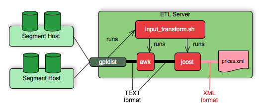
Transfer the Data
Create the target database tables with SQL statements based on the appropriate schema.
There are no special requirements for SynxDB tables that hold loaded data. In the prices example, the following command creates the prices table, where the data is to be loaded.
CREATE TABLE prices (
itemnumber integer,
price decimal
)
DISTRIBUTED BY (itemnumber);
Next, use one of the following approaches to transform the data with gpfdist.
gploadsupports only input transformations, but in many cases is easier to implement.gpfdistwithINSERT INTO SELECT FROMsupports both input and output transformations, but exposes details thatgploadautomates for you.
Transforming with gpload
The SynxDB gpload utility orchestrates a data load operation using the gpfdist parallel file server and a YAML-formatted configuration file. gpload automates these tasks:
- Creates a readable external table in the database.
- Starts
gpfdistinstances with the configuration file that contains the transformation. - Runs
INSERT INTO table\_name SELECT FROM external\_tableto load the data. - Removes the external table definition.
Transforming data with gpload requires that the settings TRANSFORM and TRANSFORM_CONFIG appear in the INPUT section of the gpload control file.
For more information about the syntax and placement of these settings in the gpload control file, see the SynxDB Reference Guide.
TRANSFORM_CONFIGspecifies the name of the gpfdist configuration file.- The
TRANSFORMsetting indicates the name of the transformation that is described in the file named inTRANSFORM_CONFIG.
---
VERSION: 1.0.0.1
DATABASE: ops
USER: gpadmin
GPLOAD:
INPUT:
- TRANSFORM_CONFIG: config.yaml
- TRANSFORM: prices_input
- SOURCE:
FILE: prices.xml
The transformation name must appear in two places: in the TRANSFORM setting of the gpfdist configuration file and in the TRANSFORMATIONS section of the file named in the TRANSFORM_CONFIG section.
In the gpload control file, the optional parameter MAX_LINE_LENGTH specifies the maximum length of a line in the XML transformation data that is passed to gpload.
The following diagram shows the relationships between the gpload control file, the gpfdist configuration file, and the XML data file.
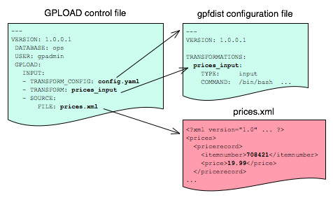
Transforming with gpfdist and INSERT INTO SELECT FROM
With this load method, you perform each of the tasks that gpload automates. You start gpfdist, create an external table, load the data, and clean up by dropping the table and stopping gpfdist.
Specify the transformation in the CREATE EXTERNAL TABLE definition’s LOCATION clause. For example, the transform is shown in bold in the following command. (Run gpfdist first, using the command gpfdist -c config.yaml).
CREATE READABLE EXTERNAL TABLE prices_readable (LIKE prices)
LOCATION ('gpfdist://hostname:8080/prices.xml#transform=prices_input')
FORMAT 'TEXT' (DELIMITER '|')
LOG ERRORS SEGMENT REJECT LIMIT 10;
In the command above, change hostname to your hostname. prices_input comes from the gpfdist configuration file.
The following query then loads the data into the prices table.
INSERT INTO prices SELECT * FROM prices_readable;
Configuration File Format
The gpfdist configuration file uses the YAML 1.1 document format and implements a schema for defining the transformation parameters. The configuration file must be a valid YAML document.
The gpfdist program processes the document in order and uses indentation (spaces) to determine the document hierarchy and relationships of the sections to one another. The use of white space is significant. Do not use white space for formatting and do not use tabs.
The following is the basic structure of a configuration file.
---
VERSION: 1.0.0.1
TRANSFORMATIONS:
transformation_name1:
TYPE: input | output
COMMAND: command
CONTENT: data | paths
SAFE: posix-regex
STDERR: server | console
transformation_name2:
TYPE: input | output
COMMAND: command
...
VERSION : Required. The version of the gpfdist configuration file schema. The current version is 1.0.0.1.
TRANSFORMATIONS : Required. Begins the transformation specification section. A configuration file must have at least one transformation. When gpfdist receives a transformation request, it looks in this section for an entry with the matching transformation name.
TYPE
: Required. Specifies the direction of transformation. Values are input or output.
input: gpfdist treats the standard output of the transformation process as a stream of records to load into SynxDB.output: gpfdist treats the standard input of the transformation process as a stream of records from SynxDB to transform and write to the appropriate output.
COMMAND : Required. Specifies the command gpfdist will run to perform the transformation.
For input transformations, gpfdist invokes the command specified in the CONTENT setting. The command is expected to open the underlying file(s) as appropriate and produce one line of TEXT for each row to load into SynxDB. The input transform determines whether the entire content should be converted to one row or to multiple rows.
For output transformations, gpfdist invokes this command as specified in the CONTENT setting. The output command is expected to open and write to the underlying file(s) as appropriate. The output transformation determines the final placement of the converted output.
CONTENT
: Optional. The values are data and paths. The default value is data.
- When
CONTENTspecifiesdata, the text%filename%in theCOMMANDsection is replaced by the path to the file to read or write. - When
CONTENTspecifiespaths, the text%filename%in theCOMMANDsection is replaced by the path to the temporary file that contains the list of files to read or write.
The following is an example of a COMMAND section showing the text %filename% that is replaced.
COMMAND: /bin/bash input_transform.sh %filename%
SAFE
: Optional. A POSIX regular expression that the paths must match to be passed to the transformation. Specify SAFE when there is a concern about injection or improper interpretation of paths passed to the command. The default is no restriction on paths.
STDERR
: Optional. The values are server and console.
This setting specifies how to handle standard error output from the transformation. The default, server, specifies that gpfdist will capture the standard error output from the transformation in a temporary file and send the first 8k of that file to SynxDB as an error message. The error message will appear as an SQL error. Console specifies that gpfdist does not redirect or transmit the standard error output from the transformation.
XML Transformation Examples
The following examples demonstrate the complete process for different types of XML data and STX transformations. Files and detailed instructions associated with these examples are in the GitHub repo https://github.com/apache/cloudberry in the gpMgmt/demo/gpfdist_transform directory. Read the README file in the Before You Begin section before you run the examples. The README file explains how to download the example data file used in the examples.
Command-based External Web Tables
The output of a shell command or script defines command-based web table data. Specify the command in the EXECUTE clause of CREATE EXTERNAL WEB TABLE. The data is current as of the time the command runs. The EXECUTE clause runs the shell command or script on the specified master, and/or segment host or hosts. The command or script must reside on the hosts corresponding to the host(s) defined in the EXECUTE clause.
By default, the command is run on segment hosts when active segments have output rows to process. For example, if each segment host runs four primary segment instances that have output rows to process, the command runs four times per segment host. You can optionally limit the number of segment instances that run the web table command. All segments included in the web table definition in the ON clause run the command in parallel.
The command that you specify in the external table definition runs from the database and cannot access environment variables from .bashrc or .profile. Set environment variables in the EXECUTE clause. For example:
=# CREATE EXTERNAL WEB TABLE output (output text)
EXECUTE 'PATH=/home/gpadmin/programs; export PATH; myprogram.sh'
FORMAT 'TEXT';
Scripts must be executable by the gpadmin user and reside in the same location on the master or segment hosts.
The following command defines a web table that runs a script. The script runs on each segment host where a segment has output rows to process.
=# CREATE EXTERNAL WEB TABLE log_output
(linenum int, message text)
EXECUTE '/var/load_scripts/get_log_data.sh' ON HOST
FORMAT 'TEXT' (DELIMITER '|');
IRS MeF XML Files (In demo Directory)
This example demonstrates loading a sample IRS Modernized eFile tax return using a Joost STX transformation. The data is in the form of a complex XML file.
The U.S. Internal Revenue Service (IRS) made a significant commitment to XML and specifies its use in its Modernized e-File (MeF) system. In MeF, each tax return is an XML document with a deep hierarchical structure that closely reflects the particular form of the underlying tax code.
XML, XML Schema and stylesheets play a role in their data representation and business workflow. The actual XML data is extracted from a ZIP file attached to a MIME “transmission file” message. For more information about MeF, see Modernized e-File (Overview) on the IRS web site.
The sample XML document, RET990EZ_2006.xml, is about 350KB in size with two elements:
- ReturnHeader
- ReturnData
The <ReturnHeader> element contains general details about the tax return such as the taxpayer’s name, the tax year of the return, and the preparer. The <ReturnData> element contains multiple sections with specific details about the tax return and associated schedules.
The following is an abridged sample of the XML file.
<?xml version="1.0" encoding="UTF-8"?>
<Return returnVersion="2006v2.0"
xmlns="https://www.irs.gov/efile"
xmlns:efile="https://www.irs.gov/efile"
xsi:schemaLocation="https://www.irs.gov/efile"
xmlns:xsi="http://www.w3.org/2001/XMLSchema-instance">
<ReturnHeader binaryAttachmentCount="1">
<ReturnId>AAAAAAAAAAAAAAAAAAAA</ReturnId>
<Timestamp>1999-05-30T12:01:01+05:01</Timestamp>
<ReturnType>990EZ</ReturnType>
<TaxPeriodBeginDate>2005-01-01</TaxPeriodBeginDate>
<TaxPeriodEndDate>2005-12-31</TaxPeriodEndDate>
<Filer>
<EIN>011248772</EIN>
... more data ...
</Filer>
<Preparer>
<Name>Percy Polar</Name>
... more data ...
</Preparer>
<TaxYear>2005</TaxYear>
</ReturnHeader>
... more data ..
The goal is to import all the data into a SynxDB database. First, convert the XML document into text with newlines “escaped”, with two columns: ReturnId and a single column on the end for the entire MeF tax return. For example:
AAAAAAAAAAAAAAAAAAAA|<Return returnVersion="2006v2.0"...
Load the data into SynxDB.
WITSML™ Files (In demo Directory)
This example demonstrates loading sample data describing an oil rig using a Joost STX transformation. The data is in the form of a complex XML file downloaded from energistics.org.
The Wellsite Information Transfer Standard Markup Language (WITSML™) is an oil industry initiative to provide open, non-proprietary, standard interfaces for technology and software to share information among oil companies, service companies, drilling contractors, application vendors, and regulatory agencies. For more information about WITSML™, see https://www.energistics.org/.
The oil rig information consists of a top level <rigs> element with multiple child elements such as <documentInfo>, <rig>, and so on. The following excerpt from the file shows the type of information in the <rig> tag.
<?xml version="1.0" encoding="UTF-8"?>
<?xml-stylesheet href="../stylesheets/rig.xsl" type="text/xsl" media="screen"?>
<rigs
xmlns="https://www.energistics.org/schemas/131"
xmlns:xsi="https://www.w3.org/2001/XMLSchema-instance"
xsi:schemaLocation="https://www.energistics.org/schemas/131 ../obj_rig.xsd"
version="1.3.1.1">
<documentInfo>
... misc data ...
</documentInfo>
<rig uidWell="W-12" uidWellbore="B-01" uid="xr31">
<nameWell>6507/7-A-42</nameWell>
<nameWellbore>A-42</nameWellbore>
<name>Deep Drill #5</name>
<owner>Deep Drilling Co.</owner>
<typeRig>floater</typeRig>
<manufacturer>Fitsui Engineering</manufacturer>
<yearEntService>1980</yearEntService>
<classRig>ABS Class A1 M CSDU AMS ACCU</classRig>
<approvals>DNV</approvals>
... more data ...
The goal is to import the information for this rig into SynxDB.
The sample document, rig.xml, is about 11KB in size. The input does not contain tabs so the relevant information can be converted into records delimited with a pipe (|).
W-12|6507/7-A-42|xr31|Deep Drill #5|Deep Drilling Co.|John Doe|John.Doe@example.com|
With the columns:
well_uid text, – e.g. W-12well_name text, – e.g. 6507/7-A-42rig_uid text, – e.g. xr31rig_name text, – e.g. Deep Drill #5rig_owner text, – e.g. Deep Drilling Co.rig_contact text, – e.g. John Doerig_email text, – e.g. John.Doe@example.comdoc xml
Then, load the data into SynxDB.
Loading Data with COPY
COPY FROM copies data from a file or standard input into a table and appends the data to the table contents. COPY is non-parallel: data is loaded in a single process using the SynxDB master instance. Using COPY is only recommended for very small data files.
The COPY source file must be accessible to the postgres process on the master host. Specify the COPY source file name relative to the data directory on the master host, or specify an absolute path.
SynxDB copies data from STDIN or STDOUT using the connection between the client and the master server.
Loading From a File
The COPY command asks the postgres backend to open the specified file, read it and append it to the table. In order to be able to read the file, the backend needs to have read permissions on the file, and the file name must be specified using an absolute path on the master host, or a relative path to the master data directory.
COPY <table_name> FROM </path/to/filename>;
Loading From STDIN
To avoid the problem of copying the data file to the master host before loading the data, COPY FROM STDIN uses the Standard Input channel and feeds data directly into the postgres backend. After the COPY FROM STDIN command started, the backend will accept lines of data until a single line only contains a backslash-period (\.).
COPY <table_name> FROM <STDIN>;
Loading Data Using \copy in psql
Do not confuse the psql \copy command with the COPY SQL command. The \copy invokes a regular COPY FROM STDIN and sends the data from the psql client to the backend. Therefore any file must reside on the host where the psql client runs, and must be accessible to the user which runs the client.
To avoid the problem of copying the data file to the master host before loading the data, COPY FROM STDIN uses the Standard Input channel and feeds data directly into the postgres backend. After the COPY FROM STDIN command started, the backend will accept lines of data until a single line only contains a backslash-period (\.). psql is wrapping all of this into the handy \copy command.
\copy <table_name> FROM <filename>;
Input Format
COPY FROM accepts a FORMAT parameter, which specifies the format of the input data. The possible values are TEXT, CSV (Comma Separated Values), and BINARY.
COPY <table_name> FROM </path/to/filename> WITH (FORMAT csv);
The FORMAT csv will read comma-separated values. The FORMAT text by default uses tabulators to separate the values, the DELIMITER option specifies a different character as value delimiter.
COPY <table_name> FROM </path/to/filename> WITH (FORMAT text, DELIMITER '|');
By default, the default client encoding is used, this can be changed with the ENCODING option. This is useful if data is coming from another operating system.
COPY <table_name> FROM </path/to/filename> WITH (ENCODING 'latin1');
Running COPY in Single Row Error Isolation Mode
By default, COPY stops an operation at the first error: if the data contains an error, the operation fails and no data loads. If you run COPY FROM in single row error isolation mode, SynxDB skips rows that contain format errors and loads properly formatted rows. Single row error isolation mode applies only to rows in the input file that contain format errors. If the data contains a constraint error such as violation of a NOT NULL, CHECK, or UNIQUE constraint, the operation fails and no data loads.
Specifying SEGMENT REJECT LIMIT runs the COPY operation in single row error isolation mode. Specify the acceptable number of error rows on each segment, after which the entire COPY FROM operation fails and no rows load. The error row count is for each SynxDB segment, not for the entire load operation.
If the COPY operation does not reach the error limit, SynxDB loads all correctly-formatted rows and discards the error rows. Use the LOG ERRORS clause to capture data formatting errors internally in SynxDB. For example:
=> COPY country FROM '/data/gpdb/country_data'
WITH DELIMITER '|' LOG ERRORS
SEGMENT REJECT LIMIT 10 ROWS;
See Viewing Bad Rows in the Error Log for information about investigating error rows.
Optimizing Data Load and Query Performance
Use the following tips to help optimize your data load and subsequent query performance.
-
Drop indexes before loading data into existing tables.
Creating an index on pre-existing data is faster than updating it incrementally as each row is loaded. You can temporarily increase the
maintenance_work_memserver configuration parameter to help speed upCREATE INDEXcommands, though load performance is affected. Drop and recreate indexes only when there are no active users on the system. -
Create indexes last when loading data into new tables. Create the table, load the data, and create any required indexes.
-
Run
ANALYZEafter loading data. If you significantly altered the data in a table, runANALYZEorVACUUM ANALYZEto update table statistics for the query optimizer. Current statistics ensure that the optimizer makes the best decisions during query planning and avoids poor performance due to inaccurate or nonexistent statistics. -
Run
VACUUMafter load errors. If the load operation does not run in single row error isolation mode, the operation stops at the first error. The target table contains the rows loaded before the error occurred. You cannot access these rows, but they occupy disk space. Use theVACUUMcommand to recover the wasted space.
Unloading Data from SynxDB
A writable external table allows you to select rows from other database tables and output the rows to files, named pipes, to applications, or as output targets for SynxDB parallel MapReduce calculations. You can define file-based and web-based writable external tables.
This topic describes how to unload data from SynxDB using parallel unload (writable external tables) and non-parallel unload (COPY).
Defining a File-Based Writable External Table
Writable external tables that output data to files can use the SynxDB parallel file server program, gpfdist, or the SynxDB Platform Extension Framework (PXF), SynxDB’s interface to Hadoop.
Use the CREATE WRITABLE EXTERNAL TABLE command to define the external table and specify the location and format of the output files. See Using the SynxDB Parallel File Server (gpfdist) for instructions on setting up gpfdist for use with an external table and Accessing External Data with PXF for instructions on setting up PXF for use with an external table
- With a writable external table using the gpfdist protocol, the SynxDB segments send their data to gpfdist, which writes the data to the named file. gpfdist must run on a host that the SynxDB segments can access over the network. gpfdist points to a file location on the output host and writes data received from the SynxDB segments to the file. To divide the output data among multiple files, list multiple gpfdist URIs in your writable external table definition.
- A writable external web table sends data to an application as a stream of data. For example, unload data from SynxDB and send it to an application that connects to another database or ETL tool to load the data elsewhere. Writable external web tables use the
EXECUTEclause to specify a shell command, script, or application to run on the segment hosts and accept an input stream of data. See Defining a Command-Based Writable External Web Table for more information about usingEXECUTEcommands in a writable external table definition.
You can optionally declare a distribution policy for your writable external tables. By default, writable external tables use a random distribution policy. If the source table you are exporting data from has a hash distribution policy, defining the same distribution key column(s) for the writable external table improves unload performance by eliminating the requirement to move rows over the interconnect. If you unload data from a particular table, you can use the LIKE clause to copy the column definitions and distribution policy from the source table.
Example 1—SynxDB file server (gpfdist)
=# CREATE WRITABLE EXTERNAL TABLE unload_expenses
( LIKE expenses )
LOCATION ('gpfdist://etlhost-1:8081/expenses1.out',
'gpfdist://etlhost-2:8081/expenses2.out')
FORMAT 'TEXT' (DELIMITER ',')
DISTRIBUTED BY (exp_id);
Example 2—Hadoop file server (pxf)
=# CREATE WRITABLE EXTERNAL TABLE unload_expenses
( LIKE expenses )
LOCATION ('pxf://dir/path?PROFILE=hdfs:text')
FORMAT 'TEXT' (DELIMITER ',')
DISTRIBUTED BY (exp_id);
You specify an HDFS directory for a writable external table that you create with the pxf protocol.
Defining a Command-Based Writable External Web Table
You can define writable external web tables to send output rows to an application or script. The application must accept an input stream, reside in the same location on all of the SynxDB segment hosts, and be executable by the gpadmin user. All segments in the SynxDB system run the application or script, whether or not a segment has output rows to process.
Use CREATE WRITABLE EXTERNAL WEB TABLE to define the external table and specify the application or script to run on the segment hosts. Commands run from within the database and cannot access environment variables (such as $PATH). Set environment variables in the EXECUTE clause of your writable external table definition. For example:
=# CREATE WRITABLE EXTERNAL WEB TABLE output (output text)
EXECUTE 'export PATH=$PATH:/home/`gpadmin`
/programs;
myprogram.sh'
FORMAT 'TEXT'
DISTRIBUTED RANDOMLY;
The following SynxDB variables are available for use in OS commands run by a web or writable external table. Set these variables as environment variables in the shell that runs the command(s). They can be used to identify a set of requests made by an external table statement across the SynxDB array of hosts and segment instances.
| Variable | Description |
|---|---|
| $GP_CID | Command count of the transaction running the external table statement. |
| $GP_DATABASE | The database in which the external table definition resides. |
| $GP_DATE | The date on which the external table command ran. |
| $GP_MASTER_HOST | The host name of the SynxDB master host from which the external table statement was dispatched. |
| $GP_MASTER_PORT | The port number of the SynxDB master instance from which the external table statement was dispatched. |
| $GP_QUERY_STRING | The SQL command (DML or SQL query) run by SynxDB. |
| $GP_SEG_DATADIR | The location of the data directory of the segment instance running the external table command. |
| $GP_SEG_PG_CONF | The location of the postgresql.conf file of the segment instance running the external table command. |
| $GP_SEG_PORT | The port number of the segment instance running the external table command. |
| $GP_SEGMENT_COUNT | The total number of primary segment instances in the SynxDB system. |
| $GP_SEGMENT_ID | The ID number of the segment instance running the external table command (same as content in gp_segment_configuration). |
| $GP_SESSION_ID | The database session identifier number associated with the external table statement. |
| $GP_SN | Serial number of the external table scan node in the query plan of the external table statement. |
| $GP_TIME | The time the external table command was run. |
| $GP_USER | The database user running the external table statement. |
| $GP_XID | The transaction ID of the external table statement. |
Deactivating EXECUTE for Web or Writable External Tables
There is a security risk associated with allowing external tables to run OS commands or scripts. To deactivate the use of EXECUTE in web and writable external table definitions, set the gp_external_enable_exec server configuration parameter to off in your master postgresql.conf file:
gp_external_enable_exec = off
Note You must restart the database in order for changes to the
gp_external_enable_execserver configuration parameter to take effect.
Unloading Data Using a Writable External Table
Writable external tables allow only INSERT operations. You must grant INSERT permission on a table to enable access to users who are not the table owner or a superuser. For example:
GRANT INSERT ON writable_ext_table TO admin;
To unload data using a writable external table, select the data from the source table(s) and insert it into the writable external table. The resulting rows are output to the writable external table. For example:
INSERT INTO writable_ext_table SELECT * FROM regular_table;
Unloading Data Using COPY
COPY TO copies data from a table to a file (or standard input) on the SynxDB master host using a single process on the SynxDB master instance. Use COPY to output a table’s entire contents, or filter the output using a SELECT statement. For example:
COPY (SELECT * FROM country WHERE country_name LIKE 'A%')
TO '/home/gpadmin/a_list_countries.out';
Formatting Data Files
When you use the SynxDB tools for loading and unloading data, you must specify how your data is formatted. COPY, CREATE EXTERNAL TABLE,and gpload have clauses that allow you to specify how your data is formatted. Data can be delimited text (TEXT) or comma separated values (CSV) format. External data must be formatted correctly to be read by SynxDB. This topic explains the format of data files expected by SynxDB.
Formatting Rows
SynxDB expects rows of data to be separated by the LF character (Line feed, 0x0A), CR (Carriage return, 0x0D), or CR followed by LF (CR+LF, 0x0D 0x0A). LF is the standard newline representation on UNIX or UNIX-like operating systems. Operating systems such as Windows or Mac OS X use CR or CR+LF. All of these representations of a newline are supported by SynxDB as a row delimiter. For more information, see Importing and Exporting Fixed Width Data.
Formatting Columns
The default column or field delimiter is the horizontal TAB character (0x09) for text files and the comma character (0x2C) for CSV files. You can declare a single character delimiter using the DELIMITER clause of COPY, CREATE EXTERNAL TABLE or gpload when you define your data format. The delimiter character must appear between any two data value fields. Do not place a delimiter at the beginning or end of a row. For example, if the pipe character ( | ) is your delimiter:
data value 1|data value 2|data value 3
The following command shows the use of the pipe character as a column delimiter:
=# CREATE EXTERNAL TABLE ext_table (name text, date date)
LOCATION ('gpfdist://<hostname>/filename.txt)
FORMAT 'TEXT' (DELIMITER '|');
Representing NULL Values
NULL represents an unknown piece of data in a column or field. Within your data files you can designate a string to represent null values. The default string is \N (backslash-N) in TEXT mode, or an empty value with no quotations in CSV mode. You can also declare a different string using the NULL clause of COPY, CREATE EXTERNAL TABLEor gpload when defining your data format. For example, you can use an empty string if you do not want to distinguish nulls from empty strings. When using the SynxDB loading tools, any data item that matches the designated null string is considered a null value.
Escaping
There are two reserved characters that have special meaning to SynxDB:
- The designated delimiter character separates columns or fields in the data file.
- The newline character designates a new row in the data file.
If your data contains either of these characters, you must escape the character so that SynxDB treats it as data and not as a field separator or new row. By default, the escape character is a \ (backslash) for text-formatted files and a double quote (“) for csv-formatted files.
Escaping in Text Formatted Files
By default, the escape character is a \ (backslash) for text-formatted files. You can declare a different escape character in the ESCAPE clause of COPY, CREATE EXTERNAL TABLEor gpload. If your escape character appears in your data, use it to escape itself.
For example, suppose you have a table with three columns and you want to load the following three fields:
backslash = \vertical bar = |exclamation point = !
Your designated delimiter character is | (pipe character), and your designated escape character is \ (backslash). The formatted row in your data file looks like this:
backslash = \\ | vertical bar = \| | exclamation point = !
Notice how the backslash character that is part of the data is escaped with another backslash character, and the pipe character that is part of the data is escaped with a backslash character.
You can use the escape character to escape octal and hexadecimal sequences. The escaped value is converted to the equivalent character when loaded into SynxDB. For example, to load the ampersand character (&), use the escape character to escape its equivalent hexadecimal (\0x26) or octal (\046) representation.
You can deactivate escaping in TEXT-formatted files using the ESCAPE clause of COPY, CREATE EXTERNAL TABLEor gpload as follows:
ESCAPE 'OFF'
This is useful for input data that contains many backslash characters, such as web log data.
Escaping in CSV Formatted Files
By default, the escape character is a " (double quote) for CSV-formatted files. If you want to use a different escape character, use the ESCAPE clause of COPY, CREATE EXTERNAL TABLE or gpload to declare a different escape character. In cases where your selected escape character is present in your data, you can use it to escape itself.
For example, suppose you have a table with three columns and you want to load the following three fields:
Free trip to A,B5.89Special rate "1.79"
Your designated delimiter character is , (comma), and your designated escape character is " (double quote). The formatted row in your data file looks like this:
"Free trip to A,B","5.89","Special rate ""1.79"""
The data value with a comma character that is part of the data is enclosed in double quotes. The double quotes that are part of the data are escaped with a double quote even though the field value is enclosed in double quotes.
Embedding the entire field inside a set of double quotes guarantees preservation of leading and trailing whitespace characters:
"Free trip to A,B ","5.89 ","Special rate ""1.79"" "
Note In CSV mode, all characters are significant. A quoted value surrounded by white space, or any characters other than
DELIMITER, includes those characters. This can cause errors if you import data from a system that pads CSV lines with white space to some fixed width. In this case, preprocess the CSV file to remove the trailing white space before importing the data into SynxDB.
Character Encoding
Character encoding systems consist of a code that pairs each character from a character set with something else, such as a sequence of numbers or octets, to facilitate data transmission and storage. SynxDB supports a variety of character sets, including single-byte character sets such as the ISO 8859 series and multiple-byte character sets such as EUC (Extended UNIX Code), UTF-8, and Mule internal code. The server-side character set is defined during database initialization, UTF-8 is the default and can be changed. Clients can use all supported character sets transparently, but a few are not supported for use within the server as a server-side encoding. When loading or inserting data into SynxDB, SynxDB transparently converts the data from the specified client encoding into the server encoding. When sending data back to the client, SynxDB converts the data from the server character encoding into the specified client encoding.
Data files must be in a character encoding recognized by SynxDB. See the SynxDB Reference Guide for the supported character sets.Data files that contain invalid or unsupported encoding sequences encounter errors when loading into SynxDB.
Note On data files generated on a Microsoft Windows operating system, run the
dos2unixsystem command to remove any Windows-only characters before loading into SynxDB.
Note If you change the
ENCODINGvalue in an existinggploadcontrol file, you must manually drop any external tables that were creating using the previousENCODINGconfiguration.gploaddoes not drop and recreate external tables to use the newENCODINGifREUSE_TABLESis set totrue.
Changing the Client-Side Character Encoding
The client-side character encoding can be changed for a session by setting the server configuration parameter client_encoding
SET client_encoding TO 'latin1';
Change the client-side character encoding back to the default value:
RESET client_encoding;
Show the current client-side character encoding setting:
SHOW client_encoding;
Example Custom Data Access Protocol
The following is the API for the SynxDB custom data access protocol. The example protocol implementation gpextprotocal.c is written in C and shows how the API can be used. For information about accessing a custom data access protocol, see Using a Custom Protocol.
/* ---- Read/Write function API ------*/
CALLED_AS_EXTPROTOCOL(fcinfo)
EXTPROTOCOL_GET_URL(fcinfo)(fcinfo)
EXTPROTOCOL_GET_DATABUF(fcinfo)
EXTPROTOCOL_GET_DATALEN(fcinfo)
EXTPROTOCOL_GET_SCANQUALS(fcinfo)
EXTPROTOCOL_GET_USER_CTX(fcinfo)
EXTPROTOCOL_IS_LAST_CALL(fcinfo)
EXTPROTOCOL_SET_LAST_CALL(fcinfo)
EXTPROTOCOL_SET_USER_CTX(fcinfo, p)
/* ------ Validator function API ------*/
CALLED_AS_EXTPROTOCOL_VALIDATOR(fcinfo)
EXTPROTOCOL_VALIDATOR_GET_URL_LIST(fcinfo)
EXTPROTOCOL_VALIDATOR_GET_NUM_URLS(fcinfo)
EXTPROTOCOL_VALIDATOR_GET_NTH_URL(fcinfo, n)
EXTPROTOCOL_VALIDATOR_GET_DIRECTION(fcinfo)
Notes
The protocol corresponds to the example described in Using a Custom Protocol. The source code file name and shared object are gpextprotocol.c and gpextprotocol.so.
The protocol has the following properties:
-
The name defined for the protocol is
myprot. -
The protocol has the following simple form: the protocol name and a path, separated by
://.myprot://path -
Three functions are implemented:
myprot_import()a read functionmyprot_export()a write functionmyprot_validate_urls()a validation function These functions are referenced in theCREATE PROTOCOLstatement when the protocol is created and declared in the database.
The example implementation gpextprotocal.c uses fopen() and fread() to simulate a simple protocol that reads local files. In practice, however, the protocol would implement functionality such as a remote connection to some process over the network.
Installing the External Table Protocol
To use the example external table protocol, you use the C compiler cc to compile and link the source code to create a shared object that can be dynamically loaded by SynxDB. The commands to compile and link the source code on a Linux system are similar to this:
cc -fpic -c gpextprotocal.c cc -shared -o gpextprotocal.so gpextprotocal.o
The option -fpic specifies creating position-independent code (PIC) and the -c option compiles the source code without linking and creates an object file. The object file needs to be created as position-independent code (PIC) so that it can be loaded at any arbitrary location in memory by SynxDB.
The flag -shared specifies creating a shared object (shared library) and the -o option specifies the shared object file name gpextprotocal.so. Refer to the GCC manual for more information on the cc options.
The header files that are declared as include files in gpextprotocal.c are located in subdirectories of $GPHOME/include/postgresql/.
For more information on compiling and linking dynamically-loaded functions and examples of compiling C source code to create a shared library on other operating systems, see the PostgreSQL documentation at https://www.postgresql.org/docs/9.4/xfunc-c.html#DFUNC.
The manual pages for the C compiler cc and the link editor ld for your operating system also contain information on compiling and linking source code on your system.
The compiled code (shared object file) for the custom protocol must be placed in the same location on every host in your SynxDB array (master and all segments). This location must also be in the LD_LIBRARY_PATH so that the server can locate the files. It is recommended to locate shared libraries either relative to $libdir (which is located at $GPHOME/lib) or through the dynamic library path (set by the dynamic_library_path server configuration parameter) on all master segment instances in the SynxDB array. You can use the SynxDB utilities gpssh and gpscp to update segments.
gpextprotocal.c
#include "postgres.h"
#include "fmgr.h"
#include "funcapi.h"
#include "access/extprotocol.h"
#include "catalog/pg_proc.h"
#include "utils/array.h"
#include "utils/builtins.h"
#include "utils/memutils.h"
/* Our chosen URI format. We can change it however needed */
typedef struct DemoUri
{
char *protocol;
char *path;
} DemoUri;
static DemoUri *ParseDemoUri(const char *uri_str);
static void FreeDemoUri(DemoUri* uri);
/* Do the module magic dance */
PG_MODULE_MAGIC;
PG_FUNCTION_INFO_V1(demoprot_export);
PG_FUNCTION_INFO_V1(demoprot_import);
PG_FUNCTION_INFO_V1(demoprot_validate_urls);
Datum demoprot_export(PG_FUNCTION_ARGS);
Datum demoprot_import(PG_FUNCTION_ARGS);
Datum demoprot_validate_urls(PG_FUNCTION_ARGS);
/* A user context that persists across calls. Can be
declared in any other way */
typedef struct {
char *url;
char *filename;
FILE *file;
} extprotocol_t;
/*
* The read function - Import data into GPDB.
*/
Datum
myprot_import(PG_FUNCTION_ARGS)
{
extprotocol_t *myData;
char *data;
int datlen;
size_t nread = 0;
/* Must be called via the external table format manager */
if (!CALLED_AS_EXTPROTOCOL(fcinfo))
elog(ERROR, "myprot_import: not called by external
protocol manager");
/* Get our internal description of the protocol */
myData = (extprotocol_t *) EXTPROTOCOL_GET_USER_CTX(fcinfo);
if(EXTPROTOCOL_IS_LAST_CALL(fcinfo))
{
/* we're done receiving data. close our connection */
if(myData && myData->file)
if(fclose(myData->file))
ereport(ERROR,
(errcode_for_file_access(),
errmsg("could not close file \"%s\": %m",
myData->filename)));
PG_RETURN_INT32(0);
}
if (myData == NULL)
{
/* first call. do any desired init */
const char *p_name = "myprot";
DemoUri *parsed_url;
char *url = EXTPROTOCOL_GET_URL(fcinfo);
myData = palloc(sizeof(extprotocol_t));
myData->url = pstrdup(url);
parsed_url = ParseDemoUri(myData->url);
myData->filename = pstrdup(parsed_url->path);
if(strcasecmp(parsed_url->protocol, p_name) != 0)
elog(ERROR, "internal error: myprot called with a
different protocol (%s)",
parsed_url->protocol);
FreeDemoUri(parsed_url);
/* open the destination file (or connect to remote server in
other cases) */
myData->file = fopen(myData->filename, "r");
if (myData->file == NULL)
ereport(ERROR,
(errcode_for_file_access(),
errmsg("myprot_import: could not open file \"%s\"
for reading: %m",
myData->filename),
errOmitLocation(true)));
EXTPROTOCOL_SET_USER_CTX(fcinfo, myData);
}
/* ==========================================
* DO THE IMPORT
* ========================================== */
data = EXTPROTOCOL_GET_DATABUF(fcinfo);
datlen = EXTPROTOCOL_GET_DATALEN(fcinfo);
/* read some bytes (with fread in this example, but normally
in some other method over the network) */
if(datlen > 0)
{
nread = fread(data, 1, datlen, myData->file);
if (ferror(myData->file))
ereport(ERROR,
(errcode_for_file_access(),
errmsg("myprot_import: could not write to file
\"%s\": %m",
myData->filename)));
}
PG_RETURN_INT32((int)nread);
}
/*
* Write function - Export data out of GPDB
*/
Datum
myprot_export(PG_FUNCTION_ARGS)
{
extprotocol_t *myData;
char *data;
int datlen;
size_t wrote = 0;
/* Must be called via the external table format manager */
if (!CALLED_AS_EXTPROTOCOL(fcinfo))
elog(ERROR, "myprot_export: not called by external
protocol manager");
/* Get our internal description of the protocol */
myData = (extprotocol_t *) EXTPROTOCOL_GET_USER_CTX(fcinfo);
if(EXTPROTOCOL_IS_LAST_CALL(fcinfo))
{
/* we're done sending data. close our connection */
if(myData && myData->file)
if(fclose(myData->file))
ereport(ERROR,
(errcode_for_file_access(),
errmsg("could not close file \"%s\": %m",
myData->filename)));
PG_RETURN_INT32(0);
}
if (myData == NULL)
{
/* first call. do any desired init */
const char *p_name = "myprot";
DemoUri *parsed_url;
char *url = EXTPROTOCOL_GET_URL(fcinfo);
myData = palloc(sizeof(extprotocol_t));
myData->url = pstrdup(url);
parsed_url = ParseDemoUri(myData->url);
myData->filename = pstrdup(parsed_url->path);
if(strcasecmp(parsed_url->protocol, p_name) != 0)
elog(ERROR, "internal error: myprot called with a
different protocol (%s)",
parsed_url->protocol);
FreeDemoUri(parsed_url);
/* open the destination file (or connect to remote server in
other cases) */
myData->file = fopen(myData->filename, "a");
if (myData->file == NULL)
ereport(ERROR,
(errcode_for_file_access(),
errmsg("myprot_export: could not open file \"%s\"
for writing: %m",
myData->filename),
errOmitLocation(true)));
EXTPROTOCOL_SET_USER_CTX(fcinfo, myData);
}
/* ========================================
* DO THE EXPORT
* ======================================== */
data = EXTPROTOCOL_GET_DATABUF(fcinfo);
datlen = EXTPROTOCOL_GET_DATALEN(fcinfo);
if(datlen > 0)
{
wrote = fwrite(data, 1, datlen, myData->file);
if (ferror(myData->file))
ereport(ERROR,
(errcode_for_file_access(),
errmsg("myprot_import: could not read from file
\"%s\": %m",
myData->filename)));
}
PG_RETURN_INT32((int)wrote);
}
Datum
myprot_validate_urls(PG_FUNCTION_ARGS)
{
List *urls;
int nurls;
int i;
ValidatorDirection direction;
/* Must be called via the external table format manager */
if (!CALLED_AS_EXTPROTOCOL_VALIDATOR(fcinfo))
elog(ERROR, "myprot_validate_urls: not called by external
protocol manager");
nurls = EXTPROTOCOL_VALIDATOR_GET_NUM_URLS(fcinfo);
urls = EXTPROTOCOL_VALIDATOR_GET_URL_LIST(fcinfo);
direction = EXTPROTOCOL_VALIDATOR_GET_DIRECTION(fcinfo);
/*
* Dumb example 1: search each url for a substring
* we don't want to be used in a url. in this example
* it's 'secured_directory'.
*/
for (i = 1 ; i <= nurls ; i++)
{
char *url = EXTPROTOCOL_VALIDATOR_GET_NTH_URL(fcinfo, i);
if (strstr(url, "secured_directory") != 0)
{
ereport(ERROR,
(errcode(ERRCODE_PROTOCOL_VIOLATION),
errmsg("using 'secured_directory' in a url
isn't allowed ")));
}
}
/*
* Dumb example 2: set a limit on the number of urls
* used. In this example we limit readable external
* tables that use our protocol to 2 urls max.
*/
if(direction == EXT_VALIDATE_READ && nurls > 2)
{
ereport(ERROR,
(errcode(ERRCODE_PROTOCOL_VIOLATION),
errmsg("more than 2 urls aren't allowed in this protocol ")));
}
PG_RETURN_VOID();
}
/* --- utility functions --- */
static
DemoUri *ParseDemoUri(const char *uri_str)
{
DemoUri *uri = (DemoUri *) palloc0(sizeof(DemoUri));
int protocol_len;
uri->path = NULL;
uri->protocol = NULL;
/*
* parse protocol
*/
char *post_protocol = strstr(uri_str, "://");
if(!post_protocol)
{
ereport(ERROR,
(errcode(ERRCODE_SYNTAX_ERROR),
errmsg("invalid protocol URI \'%s\'", uri_str),
errOmitLocation(true)));
}
protocol_len = post_protocol - uri_str;
uri->protocol = (char *)palloc0(protocol_len + 1);
strncpy(uri->protocol, uri_str, protocol_len);
/* make sure there is more to the uri string */
if (strlen(uri_str) <= protocol_len)
ereport(ERROR,
(errcode(ERRCODE_SYNTAX_ERROR),
errmsg("invalid myprot URI \'%s\' : missing path",
uri_str),
errOmitLocation(true)));
/* parse path */
uri->path = pstrdup(uri_str + protocol_len + strlen("://"));
return uri;
}
static
void FreeDemoUri(DemoUri *uri)
{
if (uri->path)
pfree(uri->path);
if (uri->protocol)
pfree(uri->protocol);
pfree(uri);
}
Querying Data
This topic provides information about using SQL in SynxDB databases.
You enter SQL statements called queries to view, change, and analyze data in a database using the psql interactive SQL client and other client tools.
- About SynxDB Query Processing
This topic provides an overview of how SynxDB processes queries. Understanding this process can be useful when writing and tuning queries. - About GPORCA
In SynxDB, the default GPORCA optimizer co-exists with the Postgres Planner. - Defining Queries
SynxDB is based on the PostgreSQL implementation of the SQL standard. - WITH Queries (Common Table Expressions)
TheWITHclause provides a way to use subqueries or perform a data modifying operation in a largerSELECTquery. You can also use theWITHclause in anINSERT,UPDATE, orDELETEcommand. - Using Functions and Operators
Description of user-defined and built-in functions and operators in SynxDB. - Working with JSON Data
SynxDB supports thejsonandjsonbdata types that store JSON (JavaScript Object Notation) data. - Working with XML Data
SynxDB supports thexmldata type that stores XML data. - Using Full Text Search
SynxDB provides data types, functions, operators, index types, and configurations for querying natural language documents. - Using SynxDB MapReduce
MapReduce is a programming model developed by Google for processing and generating large data sets on an array of commodity servers. SynxDB MapReduce allows programmers who are familiar with the MapReduce model to write map and reduce functions and submit them to the SynxDB parallel engine for processing. - Query Performance
SynxDB dynamically eliminates irrelevant partitions in a table and optimally allocates memory for different operators in a query. - Managing Spill Files Generated by Queries
SynxDB creates spill files, also known as workfiles, on disk if it does not have sufficient memory to run an SQL query in memory. - Query Profiling
Examine the query plans of poorly performing queries to identify possible performance tuning opportunities.
About SynxDB Query Processing
This topic provides an overview of how SynxDB processes queries. Understanding this process can be useful when writing and tuning queries.
Users issue queries to SynxDB as they would to any database management system. They connect to the database instance on the SynxDB master host using a client application such as psql and submit SQL statements.
Understanding Query Planning and Dispatch
The master receives, parses, and optimizes the query. The resulting query plan is either parallel or targeted. The master dispatches parallel query plans to all segments, as shown in Figure 1. The master dispatches targeted query plans to a single segment, as shown in Figure 2. Each segment is responsible for running local database operations on its own set of data.
Most database operations—such as table scans, joins, aggregations, and sorts—run across all segments in parallel. Each operation is performed on a segment database independent of the data stored in the other segment databases.

Certain queries may access only data on a single segment, such as single-row INSERT, UPDATE, DELETE, or SELECT operations or queries that filter on the table distribution key column(s). In queries such as these, the query plan is not dispatched to all segments, but is targeted at the segment that contains the affected or relevant row(s).

Understanding SynxDB Query Plans
A query plan is the set of operations SynxDB will perform to produce the answer to a query. Each node or step in the plan represents a database operation such as a table scan, join, aggregation, or sort. Plans are read and run from bottom to top.
In addition to common database operations such as table scans, joins, and so on, SynxDB has an additional operation type called motion. A motion operation involves moving tuples between the segments during query processing. Note that not every query requires a motion. For example, a targeted query plan does not require data to move across the interconnect.
To achieve maximum parallelism during query runtime, SynxDB divides the work of the query plan into slices. A slice is a portion of the plan that segments can work on independently. A query plan is sliced wherever a motion operation occurs in the plan, with one slice on each side of the motion.
For example, consider the following simple query involving a join between two tables:
SELECT customer, amount
FROM sales JOIN customer USING (cust_id)
WHERE dateCol = '04-30-2016';
Figure 3 shows the query plan. Each segment receives a copy of the query plan and works on it in parallel.
The query plan for this example has a redistribute motion that moves tuples between the segments to complete the join. The redistribute motion is necessary because the customer table is distributed across the segments by cust_id, but the sales table is distributed across the segments by sale_id. To perform the join, the sales tuples must be redistributed by cust_id. The plan is sliced on either side of the redistribute motion, creating slice 1 and slice 2.
This query plan has another type of motion operation called a gather motion. A gather motion is when the segments send results back up to the master for presentation to the client. Because a query plan is always sliced wherever a motion occurs, this plan also has an implicit slice at the very top of the plan (slice 3). Not all query plans involve a gather motion. For example, a CREATE TABLE x AS SELECT... statement would not have a gather motion because tuples are sent to the newly created table, not to the master.

Understanding Parallel Query Execution
SynxDB creates a number of database processes to handle the work of a query. On the master, the query worker process is called the query dispatcher (QD). The QD is responsible for creating and dispatching the query plan. It also accumulates and presents the final results. On the segments, a query worker process is called a query executor (QE). A QE is responsible for completing its portion of work and communicating its intermediate results to the other worker processes.
There is at least one worker process assigned to each slice of the query plan. A worker process works on its assigned portion of the query plan independently. During query runtime, each segment will have a number of processes working on the query in parallel.
Related processes that are working on the same slice of the query plan but on different segments are called gangs. As a portion of work is completed, tuples flow up the query plan from one gang of processes to the next. This inter-process communication between the segments is referred to as the interconnect component of SynxDB.
Figure 4 shows the query worker processes on the master and two segment instances for the query plan illustrated in Figure 3.

About GPORCA
In SynxDB, the default GPORCA optimizer co-exists with the Postgres Planner.
- Overview of GPORCA
GPORCA extends the planning and optimization capabilities of the Postgres Planner. - Activating and Deactivating GPORCA
By default, SynxDB uses GPORCA instead of the Postgres Planner. Server configuration parameters activate or deactivate GPORCA. - Collecting Root Partition Statistics
For a partitioned table, GPORCA uses statistics of the table root partition to generate query plans. These statistics are used for determining the join order, for splitting and joining aggregate nodes, and for costing the query steps. In contrast, the Postgres Planner uses the statistics of each leaf partition. - Considerations when Using GPORCA
To run queries optimally with GPORCA, consider the query criteria closely. - GPORCA Features and Enhancements
GPORCA, the SynxDB next generation query optimizer, includes enhancements for specific types of queries and operations: - Changed Behavior with GPORCA
There are changes to SynxDB behavior with the GPORCA optimizer enabled (the default) as compared to the Postgres Planner. - GPORCA Limitations
There are limitations in SynxDB when using the default GPORCA optimizer. GPORCA and the Postgres Planner currently coexist in SynxDB because GPORCA does not support all SynxDB features. - Determining the Query Optimizer that is Used
When GPORCA is enabled (the default), you can determine if SynxDB is using GPORCA or is falling back to the Postgres Planner. - About Uniform Multi-level Partitioned Tables
Overview of GPORCA
GPORCA extends the planning and optimization capabilities of the Postgres Planner.GPORCA is extensible and achieves better optimization in multi-core architecture environments. SynxDB uses GPORCA by default to generate an execution plan for a query when possible.
GPORCA also enhances SynxDB query performance tuning in the following areas:
- Queries against partitioned tables
- Queries that contain a common table expression (CTE)
- Queries that contain subqueries
In SynxDB, GPORCA co-exists with the Postgres Planner. By default, SynxDB uses GPORCA. If GPORCA cannot be used, then the Postgres Planner is used.
The following figure shows how GPORCA fits into the query planning architecture.
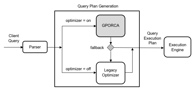
Note All Postgres Planner server configuration parameters are ignored by GPORCA. However, if SynxDB falls back to the Postgres Planner, the planner server configuration parameters will impact the query plan generation. For a list of Postgres Planner server configuration parameters, see Query Tuning Parameters.
Activating and Deactivating GPORCA
By default, SynxDB uses GPORCA instead of the Postgres Planner. Server configuration parameters activate or deactivate GPORCA.
Although GPORCA is on by default, you can configure GPORCA usage at the system, database, session, or query level using the optimizer parameter. Refer to one of the following sections if you want to change the default behavior:
- Enabling GPORCA for a System
- Enabling GPORCA for a Database
- Enabling GPORCA for a Session or a Query
Note You can deactivate the ability to activate or deactivate GPORCA with the server configuration parameter optimizer_control. For information about the server configuration parameters, see the SynxDB Reference Guide.
Enabling GPORCA for a System
Set the server configuration parameter optimizer for the SynxDB system.
-
Log into the SynxDB master host as
gpadmin, the SynxDB administrator. -
Set the values of the server configuration parameters. These SynxDB gpconfig utility commands sets the value of the parameters to
on:$ gpconfig -c optimizer -v on --masteronly -
Restart SynxDB. This SynxDB gpstop utility command reloads the
postgresql.conffiles of the master and segments without shutting down SynxDB.gpstop -u
Enabling GPORCA for a Database
Set the server configuration parameter optimizer for individual SynxDB databases with the ALTER DATABASE command. For example, this command enables GPORCA for the database test_db.
> ALTER DATABASE test_db SET OPTIMIZER = ON ;
Enabling GPORCA for a Session or a Query
You can use the SET command to set optimizer server configuration parameter for a session. For example, after you use the psql utility to connect to SynxDB, this SET command enables GPORCA:
> set optimizer = on ;
To set the parameter for a specific query, include the SET command prior to running the query.
Collecting Root Partition Statistics
For a partitioned table, GPORCA uses statistics of the table root partition to generate query plans. These statistics are used for determining the join order, for splitting and joining aggregate nodes, and for costing the query steps. In contrast, the Postgres Planner uses the statistics of each leaf partition.
If you run queries on partitioned tables, you should collect statistics on the root partition and periodically update those statistics to ensure that GPORCA can generate optimal query plans. If the root partition statistics are not up-to-date or do not exist, GPORCA still performs dynamic partition elimination for queries against the table. However, the query plan might not be optimal.
Running ANALYZE
By default, running the ANALYZE command on the root partition of a partitioned table samples the leaf partition data in the table, and stores the statistics for the root partition. ANALYZE collects statistics on the root and leaf partitions, including HyperLogLog (HLL) statistics on the leaf partitions. ANALYZE ROOTPARTITION collects statistics only on the root partition. The server configuration parameter optimizer_analyze_root_partition controls whether the ROOTPARTITION keyword is required to collect root statistics for the root partition of a partitioned table. See the ANALYZE command for information about collecting statistics on partitioned tables.
Keep in mind that ANALYZE always scans the entire table before updating the root partition statistics. If your table is very large, this operation can take a significant amount of time. ANALYZE ROOTPARTITION also uses an ACCESS SHARE lock that prevents certain operations, such as TRUNCATE and VACUUM operations, during runtime. For these reasons, you should schedule ANALYZE operations periodically, or when there are significant changes to leaf partition data.
Follow these best practices for running ANALYZE or ANALYZE ROOTPARTITION on partitioned tables in your system:
- Run
ANALYZE <root_partition_table_name>on a new partitioned table after adding initial data. RunANALYZE <leaf_partition_table_name>on a new leaf partition or a leaf partition where data has changed. By default, running the command on a leaf partition updates the root partition statistics if the other leaf partitions have statistics. - Update root partition statistics when you observe query performance regression in
EXPLAINplans against the table, or after significant changes to leaf partition data. For example, if you add a new leaf partition at some point after generating root partition statistics, consider runningANALYZEorANALYZE ROOTPARTITIONto update root partition statistics with the new tuples inserted from the new leaf partition. - For very large tables, run
ANALYZEorANALYZE ROOTPARTITIONonly weekly, or at some interval longer than daily. - Avoid running
ANALYZEwith no arguments, because doing so runs the command on all database tables including partitioned tables. With large databases, these globalANALYZEoperations are difficult to monitor, and it can be difficult to predict the time needed for completion. - Consider running multiple
ANALYZE <table_name>orANALYZE ROOTPARTITION <table_name>operations in parallel to speed the operation of statistics collection, if your I/O throughput can support the load. - You can also use the SynxDB utility
analyzedbto update table statistics. Usinganalyzedbensures that tables that were previously analyzed are not re-analyzed if no modifications were made to the leaf partition.
GPORCA and Leaf Partition Statistics
Although creating and maintaining root partition statistics is crucial for GPORCA query performance with partitioned tables, maintaining leaf partition statistics is also important. If GPORCA cannot generate a plan for a query against a partitioned table, then the Postgres Planner is used and leaf partition statistics are needed to produce the optimal plan for that query.
GPORCA itself also uses leaf partition statistics for any queries that access leaf partitions directly, instead of using the root partition with predicates to eliminate partitions. For example, if you know which partitions hold necessary tuples for a query, you can directly query the leaf partition table itself; in this case GPORCA uses the leaf partition statistics.
Deactivating Automatic Root Partition Statistics Collection
If you do not intend to run queries on partitioned tables with GPORCA (setting the server configuration parameter optimizer to off), then you can deactivate the automatic collection of statistics on the root partition of the partitioned table. The server configuration parameter optimizer_analyze_root_partition controls whether the ROOTPARTITION keyword is required to collect root statistics for the root partition of a partitioned table. The default setting for the parameter is on, the ANALYZE command can collect root partition statistics without the ROOTPARTITION keyword. You can deactivate automatic collection of root partition statistics by setting the parameter to off. When the value is off, you must run ANALZYE ROOTPARTITION to collect root partition statistics.
-
Log into the SynxDB master host as
gpadmin, the SynxDB administrator. -
Set the values of the server configuration parameters. These SynxDB
gpconfigutility commands sets the value of the parameters tooff:$ gpconfig -c optimizer_analyze_root_partition -v off --masteronly -
Restart SynxDB. This SynxDB
gpstoputility command reloads thepostgresql.conffiles of the master and segments without shutting down SynxDB.gpstop -u
Considerations when Using GPORCA
To run queries optimally with GPORCA, consider the query criteria closely.
Ensure the following criteria are met:
-
The table does not contain multi-column partition keys.
-
The multi-level partitioned table is a uniform multi-level partitioned table. See About Uniform Multi-level Partitioned Tables.
-
The server configuration parameter
optimizer_enable_master_only_queriesis set toonwhen running against master only tables such as the system table pg_attribute. For information about the parameter, see the SynxDB Reference Guide.Note Enabling this parameter decreases performance of short running catalog queries. To avoid this issue, set this parameter only for a session or a query.
-
Statistics have been collected on the root partition of a partitioned table.
If the partitioned table contains more than 20,000 partitions, consider a redesign of the table schema.
These server configuration parameters affect GPORCA query processing.
-
optimizer_cte_inlining_boundcontrols the amount of inlining performed for common table expression (CTE) queries (queries that contain aWHEREclause). -
optimizer_force_comprehensive_join_implementationaffects GPORCA’s consideration of nested loop join and hash join alternatives. When the value isfalse(the default), GPORCA does not consider nested loop join alternatives when a hash join is available. -
optimizer_force_multistage_aggforces GPORCA to choose a multi-stage aggregate plan for a scalar distinct qualified aggregate. When the value isoff(the default), GPORCA chooses between a one-stage and two-stage aggregate plan based on cost. -
optimizer_force_three_stage_scalar_dqaforces GPORCA to choose a plan with multistage aggregates when such a plan alternative is generated. -
optimizer_join_ordersets the query optimization level for join ordering by specifying which types of join ordering alternatives to evaluate. -
optimizer_join_order_thresholdspecifies the maximum number of join children for which GPORCA uses the dynamic programming-based join ordering algorithm. -
optimizer_nestloop_factorcontrols nested loop join cost factor to apply to during query optimization. -
optimizer_parallel_unioncontrols the amount of parallelization that occurs for queries that contain aUNIONorUNION ALLclause. When the value ison, GPORCA can generate a query plan of the child operations of aUNIONorUNION ALLoperation run in parallel on segment instances. -
optimizer_sort_factorcontrols the cost factor that GPORCA applies to sorting operations during query optimization. The cost factor can be adjusted for queries when data skew is present. -
gp_enable_relsize_collectioncontrols how GPORCA (and the Postgres Planner) handle a table without statistics. By default, GPORCA uses a default value to estimate the number of rows if statistics are not available. When this value ison, GPORCA uses the estimated size of a table if there are no statistics for the table.This parameter is ignored for a root partition of a partitioned table. If the root partition does not have statistics, GPORCA always uses the default value. You can use
ANALZYE ROOTPARTITIONto collect statistics on the root partition. See ANALYZE.
These server configuration parameters control the display and logging of information.
optimizer_print_missing_statscontrols the display of column information about columns with missing statistics for a query (default istrue)optimizer_print_optimization_statscontrols the logging of GPORCA query optimization metrics for a query (default isoff)
For information about the parameters, see the SynxDB Reference Guide.
GPORCA generates minidumps to describe the optimization context for a given query. The minidump files are used by Synx Data Labs support to analyze SynxDB issues. The information in the file is not in a format that can be easily used for debugging or troubleshooting. The minidump file is located under the master data directory and uses the following naming format:
Minidump_date_time.mdp
For information about the minidump file, see the server configuration parameter optimizer_minidump in the SynxDB Reference Guide.
When the EXPLAIN ANALYZE command uses GPORCA, the EXPLAIN plan shows only the number of partitions that are being eliminated. The scanned partitions are not shown. To show the name of the scanned partitions in the segment logs set the server configuration parameter gp_log_dynamic_partition_pruning to on. This example SET command enables the parameter.
SET gp_log_dynamic_partition_pruning = on;
GPORCA Features and Enhancements
GPORCA, the SynxDB next generation query optimizer, includes enhancements for specific types of queries and operations:
- Queries Against Partitioned Tables
- Queries that Contain Subqueries
- Queries that Contain Common Table Expressions
- DML Operation Enhancements with GPORCA
GPORCA also includes these optimization enhancements:
- Improved join ordering
- Join-Aggregate reordering
- Sort order optimization
- Data skew estimates included in query optimization
Queries Against Partitioned Tables
GPORCA includes these enhancements for queries against partitioned tables:
-
Partition elimination is improved.
-
Uniform multi-level partitioned tables are supported. For information about uniform multi-level partitioned tables, see About Uniform Multi-level Partitioned Tables
-
Query plan can contain the Partition selector operator.
-
Partitions are not enumerated in EXPLAIN plans.
For queries that involve static partition selection where the partitioning key is compared to a constant, GPORCA lists the number of partitions to be scanned in the
EXPLAINoutput under the Partition Selector operator. This example Partition Selector operator shows the filter and number of partitions selected:Partition Selector for Part_Table (dynamic scan id: 1) Filter: a > 10 Partitions selected: 1 (out of 3)For queries that involve dynamic partition selection where the partitioning key is compared to a variable, the number of partitions that are scanned will be known only during query execution. The partitions selected are not shown in the
EXPLAINoutput. -
Plan size is independent of number of partitions.
-
Out of memory errors caused by number of partitions are reduced.
This example CREATE TABLE command creates a range partitioned table.
CREATE TABLE sales(order_id int, item_id int, amount numeric(15,2),
date date, yr_qtr int)
PARTITION BY RANGE (yr_qtr) (start (201501) INCLUSIVE end (201504) INCLUSIVE,
start (201601) INCLUSIVE end (201604) INCLUSIVE,
start (201701) INCLUSIVE end (201704) INCLUSIVE,
start (201801) INCLUSIVE end (201804) INCLUSIVE,
start (201901) INCLUSIVE end (201904) INCLUSIVE,
start (202001) INCLUSIVE end (202004) INCLUSIVE);
GPORCA improves on these types of queries against partitioned tables:
-
Full table scan. Partitions are not enumerated in plans.
SELECT * FROM sales; -
Query with a constant filter predicate. Partition elimination is performed.
SELECT * FROM sales WHERE yr_qtr = 201501; -
Range selection. Partition elimination is performed.
SELECT * FROM sales WHERE yr_qtr BETWEEN 201601 AND 201704 ; -
Joins involving partitioned tables. In this example, the partitioned dimension table date_dim is joined with fact table catalog_sales:
SELECT * FROM catalog_sales WHERE date_id IN (SELECT id FROM date_dim WHERE month=12);
Queries that Contain Subqueries
GPORCA handles subqueries more efficiently. A subquery is query that is nested inside an outer query block. In the following query, the SELECT in the WHERE clause is a subquery.
SELECT * FROM part
WHERE price > (SELECT avg(price) FROM part);
GPORCA also handles queries that contain a correlated subquery (CSQ) more efficiently. A correlated subquery is a subquery that uses values from the outer query. In the following query, the price column is used in both the outer query and the subquery.
SELECT * FROM part p1 WHERE price > (SELECT avg(price) FROM part p2 WHERE p2.brand = p1.brand);
GPORCA generates more efficient plans for the following types of subqueries:
-
CSQ in the SELECT list.
SELECT *, (SELECT min(price) FROM part p2 WHERE p1.brand = p2.brand) AS foo FROM part p1; -
CSQ in disjunctive (OR) filters.
SELECT FROM part p1 WHERE p_size > 40 OR p_retailprice > (SELECT avg(p_retailprice) FROM part p2 WHERE p2.p_brand = p1.p_brand) -
Nested CSQ with skip level correlations
SELECT * FROM part p1 WHERE p1.p_partkey IN (SELECT p_partkey FROM part p2 WHERE p2.p_retailprice = (SELECT min(p_retailprice) FROM part p3 WHERE p3.p_brand = p1.p_brand) );Note Nested CSQ with skip level correlations are not supported by the Postgres Planner.
-
CSQ with aggregate and inequality. This example contains a CSQ with an inequality.
SELECT * FROM part p1 WHERE p1.p_retailprice = (SELECT min(p_retailprice) FROM part p2 WHERE p2.p_brand <> p1.p_brand); -
CSQ that must return one row.
SELECT p_partkey, (SELECT p_retailprice FROM part p2 WHERE p2.p_brand = p1.p_brand ) FROM part p1;
Queries that Contain Common Table Expressions
GPORCA handles queries that contain the WITH clause. The WITH clause, also known as a common table expression (CTE), generates temporary tables that exist only for the query. This example query contains a CTE.
WITH v AS (SELECT a, sum(b) as s FROM T where c < 10 GROUP BY a)
SELECT *FROM v AS v1 , v AS v2
WHERE v1.a <> v2.a AND v1.s < v2.s;
As part of query optimization, GPORCA can push down predicates into a CTE. For example query, GPORCA pushes the equality predicates to the CTE.
WITH v AS (SELECT a, sum(b) as s FROM T GROUP BY a)
SELECT *
FROM v as v1, v as v2, v as v3
WHERE v1.a < v2.a
AND v1.s < v3.s
AND v1.a = 10
AND v2.a = 20
AND v3.a = 30;
GPORCA can handle these types of CTEs:
-
CTE that defines one or multiple tables. In this query, the CTE defines two tables.
WITH cte1 AS (SELECT a, sum(b) as s FROM T where c < 10 GROUP BY a), cte2 AS (SELECT a, s FROM cte1 where s > 1000) SELECT * FROM cte1 as v1, cte2 as v2, cte2 as v3 WHERE v1.a < v2.a AND v1.s < v3.s; -
Nested CTEs.
WITH v AS (WITH w AS (SELECT a, b FROM foo WHERE b < 5) SELECT w1.a, w2.b FROM w AS w1, w AS w2 WHERE w1.a = w2.a AND w1.a > 2) SELECT v1.a, v2.a, v2.b FROM v as v1, v as v2 WHERE v1.a < v2.a;
DML Operation Enhancements with GPORCA
GPORCA contains enhancements for DML operations such as INSERT, UPDATE, and DELETE.
-
A DML node in a query plan is a query plan operator.
- Can appear anywhere in the plan, as a regular node (top slice only for now)
- Can have consumers
-
UPDATE operations use the query plan operator Split and supports these operations:
- UPDATE operations on the table distribution key columns.
- UPDATE operations on the table on the partition key column. This example plan shows the Split operator.
QUERY PLAN -------------------------------------------------------------- Update (cost=0.00..5.46 rows=1 width=1) -> Redistribute Motion 2:2 (slice1; segments: 2) Hash Key: a -> Result (cost=0.00..3.23 rows=1 width=48) -> Split (cost=0.00..2.13 rows=1 width=40) -> Result (cost=0.00..1.05 rows=1 width=40) -> Seq Scan on dmltest -
New query plan operator Assert is used for constraints checking.
This example plan shows the Assert operator.
QUERY PLAN ------------------------------------------------------------ Insert (cost=0.00..4.61 rows=3 width=8) -> Assert (cost=0.00..3.37 rows=3 width=24) Assert Cond: (dmlsource.a > 2) IS DISTINCT FROM false -> Assert (cost=0.00..2.25 rows=3 width=24) Assert Cond: NOT dmlsource.b IS NULL -> Result (cost=0.00..1.14 rows=3 width=24) -> Seq Scan on dmlsource
Changed Behavior with GPORCA
There are changes to SynxDB behavior with the GPORCA optimizer enabled (the default) as compared to the Postgres Planner.
-
UPDATE operations on distribution keys are allowed.
-
UPDATE operations on partitioned keys are allowed.
-
Queries against uniform partitioned tables are supported.
-
Queries against partitioned tables that are altered to use an external table as a leaf child partition fall back to the Postgres Planner.
-
Except for
INSERT, DML operations directly on partition (child table) of a partitioned table are not supported.For the
INSERTcommand, you can specify a leaf child table of the partitioned table to insert data into a partitioned table. An error is returned if the data is not valid for the specified leaf child table. Specifying a child table that is not a leaf child table is not supported. -
The command CREATE TABLE AS distributes table data randomly if the DISTRIBUTED BY clause is not specified and no primary or unique keys are specified.
-
Non-deterministic updates not allowed. The following UPDATE command returns an error.
update r set b = r.b + 1 from s where r.a in (select a from s); -
Statistics are required on the root table of a partitioned table. The ANALYZE command generates statistics on both root and individual partition tables (leaf child tables). See the ROOTPARTITION clause for ANALYZE command.
-
Additional Result nodes in the query plan:
- Query plan Assert operator.
- Query plan Partition selector operator.
- Query plan Split operator.
-
When running EXPLAIN, the query plan generated by GPORCA is different than the plan generated by the Postgres Planner.
-
SynxDB adds the log file message
Planner produced planwhen GPORCA is enabled and SynxDB falls back to the Postgres Planner to generate the query plan. -
SynxDB issues a warning when statistics are missing from one or more table columns. When running an SQL command with GPORCA, SynxDB issues a warning if the command performance could be improved by collecting statistics on a column or set of columns referenced by the command. The warning is issued on the command line and information is added to the SynxDB log file. For information about collecting statistics on table columns, see the ANALYZE command in the SynxDB Reference Guide.
GPORCA Limitations
There are limitations in SynxDB when using the default GPORCA optimizer. GPORCA and the Postgres Planner currently coexist in SynxDB because GPORCA does not support all SynxDB features.
This section describes the limitations.
Unsupported SQL Query Features
Certain query features are not supported with the default GPORCA optimizer. When an unsupported query is run, SynxDB logs this notice along with the query text:
Feature not supported by the SynxDB Query Optimizer: UTILITY command
These features are unsupported when GPORCA is enabled (the default):
- Prepared statements that have parameterized values.
- Indexed expressions (an index defined as expression based on one or more columns of the table)
- SP-GiST indexing method. GPORCA supports only B-tree, bitmap, GIN, and GiST indexes. GPORCA ignores indexes created with unsupported methods.
- External parameters
- These types of partitioned tables:
- Non-uniform partitioned tables.
- Partitioned tables that have been altered to use an external table as a leaf child partition.
- SortMergeJoin (SMJ).
- Ordered aggregates are not supported by default. You can enable GPORCA support for ordered aggregates with the optimizer_enable_orderedagg server configuration parameter.
- Grouping sets with ordered aggregates.
- Multi-argument
DISTINCTqualified aggregates, for exampleSELECT corr(DISTINCT a, b) FROM tbl1;, are not supported by default. You can enable GPORCA support for multi-argument distinct aggregates with the optimizer_enable_orderedagg server configuration parameter. - These analytics extensions:
- CUBE
- Multiple grouping sets
- These scalar operators:
- ROW
- ROWCOMPARE
- FIELDSELECT
- Aggregate functions that take set operators as input arguments.
- Multiple Distinct Qualified Aggregates, such as
SELECT count(DISTINCT a), sum(DISTINCT b) FROM foo, are not supported by default. They can be enabled with theoptimizer_enable_multiple_distinct_aggsConfiguration Parameter. - percentile_* window functions (ordered-set aggregate functions).
- Inverse distribution functions.
- Queries that run functions that are defined with the
ON MASTERorON ALL SEGMENTSattribute. - Queries that contain UNICODE characters in metadata names, such as table names, and the characters are not compatible with the host system locale.
SELECT,UPDATE, andDELETEcommands where a table name is qualified by theONLYkeyword.- Per-column collation. GPORCA supports collation only when all columns in the query use the same collation. If columns in the query use different collations, then SynxDB uses the Postgres Planner.
Performance Regressions
The following features are known performance regressions that occur with GPORCA enabled:
- Short running queries - For GPORCA, short running queries might encounter additional overhead due to GPORCA enhancements for determining an optimal query execution plan.
- ANALYZE - For GPORCA, the ANALYZE command generates root partition statistics for partitioned tables. For the Postgres Planner, these statistics are not generated.
- DML operations - For GPORCA, DML enhancements including the support of updates on partition and distribution keys might require additional overhead.
Also, enhanced functionality of the features from previous versions could result in additional time required when GPORCA runs SQL statements with the features.
Determining the Query Optimizer that is Used
When GPORCA is enabled (the default), you can determine if SynxDB is using GPORCA or is falling back to the Postgres Planner.
You can examine the EXPLAIN query plan for the query to determine which query optimizer was used by SynxDB to run the query:
-
The optimizer is listed at the end of the query plan. For example, when GPORCA generates the query plan, the query plan ends with:
Optimizer: Pivotal Optimizer (GPORCA)When SynxDB falls back to the Postgres Planner to generate the plan, the query plan ends with:
Optimizer: Postgres query optimizer -
These plan items appear only in the
EXPLAINplan output generated by GPORCA. The items are not supported in a Postgres Planner query plan.- Assert operator
- Sequence operator
- Dynamic Index Scan
- Dynamic Seq Scan
-
When a query against a partitioned table is generated by GPORCA, the
EXPLAINplan displays only the number of partitions that are being eliminated is listed. The scanned partitions are not shown. TheEXPLAINplan generated by the Postgres Planner lists the scanned partitions.
The log file contains messages that indicate which query optimizer was used. If SynxDB falls back to the Postgres Planner, a message with NOTICE information is added to the log file that indicates the unsupported feature. Also, the label Planner produced plan: appears before the query in the query execution log message when SynxDB falls back to the Postgres optimizer.
Note You can configure SynxDB to display log messages on the psql command line by setting the SynxDB server configuration parameter
client_min_messagestoLOG. See the SynxDB Reference Guide for information about the parameter.
Examples
This example shows the differences for a query that is run against partitioned tables when GPORCA is enabled.
This CREATE TABLE statement creates a table with single level partitions:
CREATE TABLE sales (trans_id int, date date,
amount decimal(9,2), region text)
DISTRIBUTED BY (trans_id)
PARTITION BY RANGE (date)
(START (date '20160101')
INCLUSIVE END (date '20170101')
EXCLUSIVE EVERY (INTERVAL '1 month'),
DEFAULT PARTITION outlying_dates );
This query against the table is supported by GPORCA and does not generate errors in the log file:
select * from sales ;
The EXPLAIN plan output lists only the number of selected partitions.
-> Partition Selector for sales (dynamic scan id: 1) (cost=10.00..100.00 rows=50 width=4)
Partitions selected: 13 (out of 13)
If a query against a partitioned table is not supported by GPORCA. SynxDB falls back to the Postgres Planner. The EXPLAIN plan generated by the Postgres Planner lists the selected partitions. This example shows a part of the explain plan that lists some selected partitions.
-> Append (cost=0.00..0.00 rows=26 width=53)
-> Seq Scan on sales2_1_prt_7_2_prt_usa sales2 (cost=0.00..0.00 rows=1 width=53)
-> Seq Scan on sales2_1_prt_7_2_prt_asia sales2 (cost=0.00..0.00 rows=1 width=53)
...
This example shows the log output when the SynxDB falls back to the Postgres Planner from GPORCA.
When this query is run, SynxDB falls back to the Postgres Planner.
explain select * from pg_class;
A message is added to the log file. The message contains this NOTICE information that indicates the reason GPORCA did not run the query:
NOTICE,""Feature not supported: Queries on master-only tables"
About Uniform Multi-level Partitioned Tables
GPORCA supports queries on a multi-level partitioned (MLP) table if the MLP table is a uniform partitioned table. A multi-level partitioned table is a partitioned table that was created with the SUBPARTITION clause. A uniform partitioned table must meet these requirements.
- The partitioned table structure is uniform. Each partition node at the same level must have the same hierarchical structure.
- The partition key constraints must be consistent and uniform. At each subpartition level, the sets of constraints on the child tables created for each branch must match.
You can display information about partitioned tables in several ways, including displaying information from these sources:
- The
pg_partitionssystem view contains information on the structure of a partitioned table. - The
pg_constraintsystem catalog table contains information on table constraints. - The psql meta command \d+ tablename displays the table constraints for child leaf tables of a partitioned table.
Example
This CREATE TABLE command creates a uniform partitioned table.
CREATE TABLE mlp (id int, year int, month int, day int,
region text)
DISTRIBUTED BY (id)
PARTITION BY RANGE ( year)
SUBPARTITION BY LIST (region)
SUBPARTITION TEMPLATE (
SUBPARTITION usa VALUES ( 'usa'),
SUBPARTITION europe VALUES ( 'europe'),
SUBPARTITION asia VALUES ( 'asia'))
( START ( 2006) END ( 2016) EVERY ( 5));
These are child tables and the partition hierarchy that are created for the table mlp. This hierarchy consists of one subpartition level that contains two branches.
mlp_1_prt_11
mlp_1_prt_11_2_prt_usa
mlp_1_prt_11_2_prt_europe
mlp_1_prt_11_2_prt_asia
mlp_1_prt_21
mlp_1_prt_21_2_prt_usa
mlp_1_prt_21_2_prt_europe
mlp_1_prt_21_2_prt_asia
The hierarchy of the table is uniform, each partition contains a set of three child tables (subpartitions). The constraints for the region subpartitions are uniform, the set of constraints on the child tables for the branch table mlp_1_prt_11 are the same as the constraints on the child tables for the branch table mlp_1_prt_21.
As a quick check, this query displays the constraints for the partitions.
WITH tbl AS (SELECT oid, partitionlevel AS level,
partitiontablename AS part
FROM pg_partitions, pg_class
WHERE tablename = 'mlp' AND partitiontablename=relname
AND partitionlevel=1 )
SELECT tbl.part, consrc
FROM tbl, pg_constraint
WHERE tbl.oid = conrelid ORDER BY consrc;
Note You will need modify the query for more complex partitioned tables. For example, the query does not account for table names in different schemas.
The consrc column displays constraints on the subpartitions. The set of region constraints for the subpartitions in mlp_1_prt_1 match the constraints for the subpartitions in mlp_1_prt_2. The constraints for year are inherited from the parent branch tables.
part | consrc
--------------------------+------------------------------------
mlp_1_prt_2_2_prt_asia | (region = 'asia'::text)
mlp_1_prt_1_2_prt_asia | (region = 'asia'::text)
mlp_1_prt_2_2_prt_europe | (region = 'europe'::text)
mlp_1_prt_1_2_prt_europe | (region = 'europe'::text)
mlp_1_prt_1_2_prt_usa | (region = 'usa'::text)
mlp_1_prt_2_2_prt_usa | (region = 'usa'::text)
mlp_1_prt_1_2_prt_asia | ((year >= 2006) AND (year < 2011))
mlp_1_prt_1_2_prt_usa | ((year >= 2006) AND (year < 2011))
mlp_1_prt_1_2_prt_europe | ((year >= 2006) AND (year < 2011))
mlp_1_prt_2_2_prt_usa | ((year >= 2011) AND (year < 2016))
mlp_1_prt_2_2_prt_asia | ((year >= 2011) AND (year < 2016))
mlp_1_prt_2_2_prt_europe | ((year >= 2011) AND (year < 2016))
(12 rows)
If you add a default partition to the example partitioned table with this command:
ALTER TABLE mlp ADD DEFAULT PARTITION def
The partitioned table remains a uniform partitioned table. The branch created for default partition contains three child tables and the set of constraints on the child tables match the existing sets of child table constraints.
In the above example, if you drop the subpartition mlp_1_prt_21_2_prt_asia and add another subpartition for the region canada, the constraints are no longer uniform.
ALTER TABLE mlp ALTER PARTITION FOR (RANK(2))
DROP PARTITION asia ;
ALTER TABLE mlp ALTER PARTITION FOR (RANK(2))
ADD PARTITION canada VALUES ('canada');
Also, if you add a partition canada under mlp_1_prt_21, the partitioning hierarchy is not uniform.
However, if you add the subpartition canada to both mlp_1_prt_21 and mlp_1_prt_11 the of the original partitioned table, it remains a uniform partitioned table.
Note Only the constraints on the sets of partitions at a partition level must be the same. The names of the partitions can be different.
Defining Queries
SynxDB is based on the PostgreSQL implementation of the SQL standard.
This topic describes how to construct SQL queries in SynxDB.
SQL Lexicon
SQL is a standard language for accessing databases. The language consists of elements that enable data storage, retrieval, analysis, viewing, manipulation, and so on. You use SQL commands to construct queries and commands that the SynxDB engine understands. SQL queries consist of a sequence of commands. Commands consist of a sequence of valid tokens in correct syntax order, terminated by a semicolon (;).
For more information about SQL commands, see SQL Command Reference.
SynxDB uses PostgreSQL’s structure and syntax, with some exceptions. For more information about SQL rules and concepts in PostgreSQL, see “SQL Syntax” in the PostgreSQL documentation.
SQL Value Expressions
SQL value expressions consist of one or more values, symbols, operators, SQL functions, and data. The expressions compare data or perform calculations and return a value as the result. Calculations include logical, arithmetic, and set operations.
The following are value expressions:
- An aggregate expression
- An array constructor
- A column reference
- A constant or literal value
- A correlated subquery
- A field selection expression
- A function call
- A new column value in an
INSERTorUPDATE - An operator invocation column reference
- A positional parameter reference, in the body of a function definition or prepared statement
- A row constructor
- A scalar subquery
- A search condition in a
WHEREclause - A target list of a
SELECTcommand - A type cast
- A value expression in parentheses, useful to group sub-expressions and override precedence
- A window expression
SQL constructs such as functions and operators are expressions but do not follow any general syntax rules. For more information about these constructs, see Using Functions and Operators.
Column References
A column reference has the form:
<correlation>.<columnname>
Here, correlation is the name of a table (possibly qualified with a schema name) or an alias for a table defined with a FROM clause or one of the keywords NEW or OLD. NEW and OLD can appear only in rewrite rules, but you can use other correlation names in any SQL statement. If the column name is unique across all tables in the query, you can omit the “correlation.” part of the column reference.
Positional Parameters
Positional parameters are arguments to SQL statements or functions that you reference by their positions in a series of arguments. For example, $1 refers to the first argument, $2 to the second argument, and so on. The values of positional parameters are set from arguments external to the SQL statement or supplied when SQL functions are invoked. Some client libraries support specifying data values separately from the SQL command, in which case parameters refer to the out-of-line data values. A parameter reference has the form:
$number
For example:
CREATE FUNCTION dept(text) RETURNS dept
AS $$ SELECT * FROM dept WHERE name = $1 $$
LANGUAGE SQL;
Here, the $1 references the value of the first function argument whenever the function is invoked.
Subscripts
If an expression yields a value of an array type, you can extract a specific element of the array value as follows:
<expression>[<subscript>]
You can extract multiple adjacent elements, called an array slice, as follows (including the brackets):
<expression>[<lower_subscript>:<upper_subscript>]
Each subscript is an expression and yields an integer value.
Array expressions usually must be in parentheses, but you can omit the parentheses when the expression to be subscripted is a column reference or positional parameter. You can concatenate multiple subscripts when the original array is multidimensional. For example (including the parentheses):
mytable.arraycolumn[4]
mytable.two_d_column[17][34]
$1[10:42]
(arrayfunction(a,b))[42]
Field Selection
If an expression yields a value of a composite type (row type), you can extract a specific field of the row as follows:
<expression>.<fieldname>
The row expression usually must be in parentheses, but you can omit these parentheses when the expression to be selected from is a table reference or positional parameter. For example:
mytable.mycolumn
$1.somecolumn
(rowfunction(a,b)).col3
A qualified column reference is a special case of field selection syntax.
Operator Invocations
Operator invocations have the following possible syntaxes:
<expression operator expression>(binary infix operator)
<operator expression>(unary prefix operator)
<expression operator>(unary postfix operator)
Where operator is an operator token, one of the key words AND, OR, or NOT, or qualified operator name in the form:
OPERATOR(<schema>.<operatorname>)
Available operators and whether they are unary or binary depends on the operators that the system or user defines. For more information about built-in operators, see Built-in Functions and Operators.
Function Calls
The syntax for a function call is the name of a function (possibly qualified with a schema name), followed by its argument list enclosed in parentheses:
function ([expression [, expression ... ]])
For example, the following function call computes the square root of 2:
sqrt(2)
See Summary of Built-in Functions for lists of the built-in functions by category. You can add custom functions, too.
Aggregate Expressions
An aggregate expression applies an aggregate function across the rows that a query selects. An aggregate function performs a calculation on a set of values and returns a single value, such as the sum or average of the set of values. The syntax of an aggregate expression is one of the following:
aggregate_name(expression [ , ... ] ) [ FILTER ( WHERE filter_clause ) ]— operates across all input rows for which the expected result value is non-null.ALLis the default.aggregate_name(ALL expression [ , ... ] ) [ FILTER ( WHERE filter_clause ) ]— operates identically to the first form becauseALLis the default.aggregate_name(DISTINCT expression [ , ... ] ) [ FILTER ( WHERE filter_clause ) ]— operates across all distinct non-null values of input rows.aggregate_name(*) [ FILTER ( WHERE filter_clause ) ]— operates on all rows with values both null and non-null. Generally, this form is most useful for thecount(*)aggregate function.
Where aggregate_name is a previously defined aggregate (possibly schema-qualified) and expression is any value expression that does not contain an aggregate expression.
For example, count(*) yields the total number of input rows, count(f1) yields the number of input rows in which f1 is non-null, andcount(distinct f1) yields the number of distinct non-null values of f1.
If FILTER is specified, then only the input rows for which the filter_clause evaluates to true are fed to the aggregate function; other rows are discarded. For example:
SELECT
count(*) AS unfiltered,
count(*) FILTER (WHERE i < 5) AS filtered
FROM generate_series(1,10) AS s(i);
unfiltered | filtered
------------+----------
10 | 4
(1 row)
For predefined aggregate functions, see Built-in Functions and Operators. You can also add custom aggregate functions.
SynxDB provides the MEDIAN aggregate function, which returns the fiftieth percentile of the PERCENTILE_CONT result and special aggregate expressions for inverse distribution functions as follows:
PERCENTILE_CONT(_percentage_) WITHIN GROUP (ORDER BY _expression_)
PERCENTILE_DISC(_percentage_) WITHIN GROUP (ORDER BY _expression_)
Currently you can use only these two expressions with the keyword WITHIN GROUP.
Limitations of Aggregate Expressions
The following are current limitations of the aggregate expressions:
- SynxDB does not support the following keywords:
ALL,DISTINCT, andOVER. See Using Functions and Operators for more details. - An aggregate expression can appear only in the result list or
HAVINGclause of aSELECTcommand. It is forbidden in other clauses, such asWHERE, because those clauses are logically evaluated before the results of aggregates form. This restriction applies to the query level to which the aggregate belongs. - When an aggregate expression appears in a subquery, the aggregate is normally evaluated over the rows of the subquery. If the aggregate’s arguments (and filter_clause if any) contain only outer-level variables, the aggregate belongs to the nearest such outer level and evaluates over the rows of that query. The aggregate expression as a whole is then an outer reference for the subquery in which it appears, and the aggregate expression acts as a constant over any one evaluation of that subquery. The restriction about appearing only in the result list or
HAVINGclause applies with respect to the query level at which the aggregate appears. See Scalar Subqueries and Using Functions and Operators. - SynxDB does not support specifying an aggregate function as an argument to another aggregate function.
- SynxDB does not support specifying a window function as an argument to an aggregate function.
Window Expressions
Window expressions allow application developers to more easily compose complex online analytical processing (OLAP) queries using standard SQL commands. For example, with window expressions, users can calculate moving averages or sums over various intervals, reset aggregations and ranks as selected column values change, and express complex ratios in simple terms.
A window expression represents the application of a window function to a window frame, which is defined with an OVER() clause. This is comparable to the type of calculation that can be done with an aggregate function and a GROUP BY clause. Unlike aggregate functions, which return a single result value for each group of rows, window functions return a result value for every row, but that value is calculated with respect to the set of rows in the window frame to which the row belongs. The OVER() clause allows dividing the rows into partitions and then further restricting the window frame by specifying which rows preceding or following the current row within its partition to include in the calculation.
SynxDB does not support specifying a window function as an argument to another window function.
The syntax of a window expression is:
window_function ( [expression [, ...]] ) [ FILTER ( WHERE filter_clause ) ] OVER ( window_specification )
Where window_function is one of the functions listed in Using Functions and Operators or a user-defined window function, expression is any value expression that does not contain a window expression, and window_specification is:
[window_name]
[PARTITION BY expression [, ...]]
[[ORDER BY expression [ASC | DESC | USING operator] [NULLS {FIRST | LAST}] [, ...]
[{RANGE | ROWS}
{ UNBOUNDED PRECEDING
| expression PRECEDING
| CURRENT ROW
| BETWEEN window_frame_bound AND window_frame_bound }]]
and where window_frame_bound can be one of:
UNBOUNDED PRECEDING
expression PRECEDING
CURRENT ROW
expression FOLLOWING
UNBOUNDED FOLLOWING
A window expression can appear only in the select list of a SELECT command. For example:
SELECT count(*) OVER(PARTITION BY customer_id), * FROM sales;
If FILTER is specified, then only the input rows for which the filter_clause evaluates to true are fed to the window function; other rows are discarded. In a window expression, a FILTER clause can be used only with a window_function that is an aggregate function.
In a window expression, the expression must contain an OVER clause. The OVER clause specifies the window frame—the rows to be processed by the window function. This syntactically distinguishes the function from a regular or aggregate function.
In a window aggregate function that is used in a window expression, SynxDB does not support a DISTINCT clause with multiple input expressions.
A window specification has the following characteristics:
- The
PARTITION BYclause defines the window partitions to which the window function is applied. If omitted, the entire result set is treated as one partition. - The
ORDER BYclause defines the expression(s) for sorting rows within a window partition. TheORDER BYclause of a window specification is separate and distinct from theORDER BYclause of a regular query expression. TheORDER BYclause is required for the window functions that calculate rankings, as it identifies the measure(s) for the ranking values. For OLAP aggregations, theORDER BYclause is required to use window frames (theROWSorRANGEclause).
Note Columns of data types without a coherent ordering, such as
time, are not good candidates for use in theORDER BYclause of a window specification.Time, with or without a specified time zone, lacks a coherent ordering because addition and subtraction do not have the expected effects. For example, the following is not generally true:x::time < x::time + '2 hour'::interval
- The
ROWSorRANGEclause defines a window frame for aggregate (non-ranking) window functions. A window frame defines a set of rows within a window partition. When a window frame is defined, the window function computes on the contents of this moving frame rather than the fixed contents of the entire window partition. Window frames are row-based (ROWS) or value-based (RANGE).
Window Examples
The following examples demonstrate using window functions with partitions and window frames.
Example 1 – Aggregate Window Function Over a Partition
The PARTITION BY list in the OVER clause divides the rows into groups, or partitions, that have the same values as the specified expressions.
This example compares employees’ salaries with the average salaries for their departments:
SELECT depname, empno, salary, avg(salary) OVER(PARTITION BY depname)
FROM empsalary;
depname | empno | salary | avg
-----------+-------+--------+-----------------------
develop | 9 | 4500 | 5020.0000000000000000
develop | 10 | 5200 | 5020.0000000000000000
develop | 11 | 5200 | 5020.0000000000000000
develop | 7 | 4200 | 5020.0000000000000000
develop | 8 | 6000 | 5020.0000000000000000
personnel | 5 | 3500 | 3700.0000000000000000
personnel | 2 | 3900 | 3700.0000000000000000
sales | 1 | 5000 | 4866.6666666666666667
sales | 3 | 4800 | 4866.6666666666666667
sales | 4 | 4800 | 4866.6666666666666667
(10 rows)
The first three output columns come from the table empsalary, and there is one output row for each row in the table. The fourth column is the average calculated on all rows that have the same depname value as the current row. Rows that share the same depname value constitute a partition, and there are three partitions in this example. The avg function is the same as the regular avg aggregate function, but the OVER clause causes it to be applied as a window function.
You can also put the window specification in a WINDOW clause and reference it in the select list. This example is equivalent to the previous query:
SELECT depname, empno, salary, avg(salary) OVER(mywindow)
FROM empsalary
WINDOW mywindow AS (PARTITION BY depname);
Defining a named window is useful when the select list has multiple window functions using the same window specification.
Example 2 – Ranking Window Function With an ORDER BY Clause
An ORDER BY clause within the OVER clause controls the order in which rows are processed by window functions. The ORDER BY list for the window function does not have to match the output order of the query. This example uses the rank() window function to rank employees’ salaries within their departments:
SELECT depname, empno, salary,
rank() OVER (PARTITION BY depname ORDER BY salary DESC)
FROM empsalary;
depname | empno | salary | rank
-----------+-------+--------+------
develop | 8 | 6000 | 1
develop | 11 | 5200 | 2
develop | 10 | 5200 | 2
develop | 9 | 4500 | 4
develop | 7 | 4200 | 5
personnel | 2 | 3900 | 1
personnel | 5 | 3500 | 2
sales | 1 | 5000 | 1
sales | 4 | 4800 | 2
sales | 3 | 4800 | 2
(10 rows)
Example 3 – Aggregate Function over a Row Window Frame
A RANGE or ROWS clause defines the window frame—a set of rows within a partition—that the window function includes in the calculation. ROWS specifies a physical set of rows to process, for example all rows from the beginning of the partition to the current row.
This example calculates a running total of employee’s salaries by department using the sum() function to total rows from the start of the partition to the current row:
SELECT depname, empno, salary,
sum(salary) OVER (PARTITION BY depname ORDER BY salary
ROWS between UNBOUNDED PRECEDING AND CURRENT ROW)
FROM empsalary ORDER BY depname, sum;
depname | empno | salary | sum
-----------+-------+--------+-------
develop | 7 | 4200 | 4200
develop | 9 | 4500 | 8700
develop | 11 | 5200 | 13900
develop | 10 | 5200 | 19100
develop | 8 | 6000 | 25100
personnel | 5 | 3500 | 3500
personnel | 2 | 3900 | 7400
sales | 4 | 4800 | 4800
sales | 3 | 4800 | 9600
sales | 1 | 5000 | 14600
(10 rows)
Example 4 – Aggregate Function for a Range Window Frame
RANGE specifies logical values based on values of the ORDER BY expression in the OVER clause. This example demonstrates the difference between ROWS and RANGE. The frame contains all rows with salary values less than or equal to the current row. Unlike the previous example, for employees with the same salary, the sum is the same and includes the salaries of all of those employees.
SELECT depname, empno, salary,
sum(salary) OVER (PARTITION BY depname ORDER BY salary
RANGE between UNBOUNDED PRECEDING AND CURRENT ROW)
FROM empsalary ORDER BY depname, sum;
depname | empno | salary | sum
-----------+-------+--------+-------
develop | 7 | 4200 | 4200
develop | 9 | 4500 | 8700
develop | 11 | 5200 | 19100
develop | 10 | 5200 | 19100
develop | 8 | 6000 | 25100
personnel | 5 | 3500 | 3500
personnel | 2 | 3900 | 7400
sales | 4 | 4800 | 9600
sales | 3 | 4800 | 9600
sales | 1 | 5000 | 14600
(10 rows)
Type Casts
A type cast specifies a conversion from one data type to another. A cast applied to a value expression of a known type is a run-time type conversion. The cast succeeds only if a suitable type conversion is defined. This differs from the use of casts with constants. A cast applied to a string literal represents the initial assignment of a type to a literal constant value, so it succeeds for any type if the contents of the string literal are acceptable input syntax for the data type.
SynxDB supports three types of casts applied to a value expression:
-
Explicit cast - SynxDB applies a cast when you explicitly specify a cast between two data types. SynxDB accepts two equivalent syntaxes for explicit type casts:
CAST ( expression AS type ) expression::typeThe
CASTsyntax conforms to SQL; the syntax using::is historical PostgreSQL usage. -
Assignment cast - SynxDB implicitly invokes a cast in assignment contexts, when assigning a value to a column of the target data type. For example, a CREATE CAST command with the
AS ASSIGNMENTclause creates a cast that is applied implicitly in the assignment context. This example assignment cast assumes thattbl1.f1is a column of typetext. TheINSERTcommand is allowed because the value is implicitly cast from theintegertotexttype.INSERT INTO tbl1 (f1) VALUES (42); -
Implicit cast - SynxDB implicitly invokes a cast in assignment or expression contexts. For example, a
CREATE CASTcommand with theAS IMPLICITclause creates an implicit cast, a cast that is applied implicitly in both the assignment and expression context. This example implicit cast assumes thattbl1.c1is a column of typeint. For the calculation in the predicate, the value ofc1is implicitly cast fromintto adecimaltype.SELECT * FROM tbl1 WHERE tbl1.c2 = (4.3 + tbl1.c1) ;
You can usually omit an explicit type cast if there is no ambiguity about the type a value expression must produce (for example, when it is assigned to a table column); the system automatically applies a type cast. SynxDB implicitly applies casts only to casts defined with a cast context of assignment or explicit in the system catalogs. Other casts must be invoked with explicit casting syntax to prevent unexpected conversions from being applied without the user’s knowledge.
You can display cast information with the psql meta-command \dC. Cast information is stored in the catalog table pg_cast, and type information is stored in the catalog table pg_type.
Scalar Subqueries
A scalar subquery is a SELECT query in parentheses that returns exactly one row with one column. Do not use a SELECT query that returns multiple rows or columns as a scalar subquery. The query runs and uses the returned value in the surrounding value expression. A correlated scalar subquery contains references to the outer query block.
Correlated Subqueries
A correlated subquery (CSQ) is a SELECT query with a WHERE clause or target list that contains references to the parent outer clause. CSQs efficiently express results in terms of results of another query. SynxDB supports correlated subqueries that provide compatibility with many existing applications. A CSQ is a scalar or table subquery, depending on whether it returns one or multiple rows. SynxDB does not support correlated subqueries with skip-level correlations.
Correlated Subquery Examples
Example 1 – Scalar correlated subquery
SELECT * FROM t1 WHERE t1.x
> (SELECT MAX(t2.x) FROM t2 WHERE t2.y = t1.y);
Example 2 – Correlated EXISTS subquery
SELECT * FROM t1 WHERE
EXISTS (SELECT 1 FROM t2 WHERE t2.x = t1.x);
SynxDB uses one of the following methods to run CSQs:
- Unnest the CSQ into join operations – This method is most efficient, and it is how SynxDB runs most CSQs, including queries from the TPC-H benchmark.
- Run the CSQ on every row of the outer query – This method is relatively inefficient, and it is how SynxDB runs queries that contain CSQs in the
SELECTlist or are connected byORconditions.
The following examples illustrate how to rewrite some of these types of queries to improve performance.
Example 3 - CSQ in the Select List
Original Query
SELECT T1.a,
(SELECT COUNT(DISTINCT T2.z) FROM t2 WHERE t1.x = t2.y) dt2
FROM t1;
Rewrite this query to perform an inner join with t1 first and then perform a left join with t1 again. The rewrite applies for only an equijoin in the correlated condition.
Rewritten Query
SELECT t1.a, dt2 FROM t1
LEFT JOIN
(SELECT t2.y AS csq_y, COUNT(DISTINCT t2.z) AS dt2
FROM t1, t2 WHERE t1.x = t2.y
GROUP BY t1.x)
ON (t1.x = csq_y);
Example 4 - CSQs connected by OR Clauses
Original Query
SELECT * FROM t1
WHERE
x > (SELECT COUNT(*) FROM t2 WHERE t1.x = t2.x)
OR x < (SELECT COUNT(*) FROM t3 WHERE t1.y = t3.y)
Rewrite this query to separate it into two parts with a union on the OR conditions.
Rewritten Query
SELECT * FROM t1
WHERE x > (SELECT count(*) FROM t2 WHERE t1.x = t2.x)
UNION
SELECT * FROM t1
WHERE x < (SELECT count(*) FROM t3 WHERE t1.y = t3.y)
To view the query plan, use EXPLAIN SELECT or EXPLAIN ANALYZE SELECT. Subplan nodes in the query plan indicate that the query will run on every row of the outer query, and the query is a candidate for rewriting. For more information about these statements, see Query Profiling.
Array Constructors
An array constructor is an expression that builds an array value from values for its member elements. A simple array constructor consists of the key word ARRAY, a left square bracket [, one or more expressions separated by commas for the array element values, and a right square bracket ]. For example,
SELECT ARRAY[1,2,3+4];
array
---------
{1,2,7}
The array element type is the common type of its member expressions, determined using the same rules as for UNION or CASE constructs.
You can build multidimensional array values by nesting array constructors. In the inner constructors, you can omit the keyword ARRAY. For example, the following two SELECT statements produce the same result:
SELECT ARRAY[ARRAY[1,2], ARRAY[3,4]];
SELECT ARRAY[[1,2],[3,4]];
array
---------------
{{1,2},{3,4}}
Since multidimensional arrays must be rectangular, inner constructors at the same level must produce sub-arrays of identical dimensions.
Multidimensional array constructor elements are not limited to a sub-ARRAY construct; they are anything that produces an array of the proper kind. For example:
CREATE TABLE arr(f1 int[], f2 int[]);
INSERT INTO arr VALUES (ARRAY[[1,2],[3,4]],
ARRAY[[5,6],[7,8]]);
SELECT ARRAY[f1, f2, '{{9,10},{11,12}}'::int[]] FROM arr;
array
------------------------------------------------
{{{1,2},{3,4}},{{5,6},{7,8}},{{9,10},{11,12}}}
You can construct an array from the results of a subquery. Write the array constructor with the keyword ARRAY followed by a subquery in parentheses. For example:
SELECT ARRAY(SELECT oid FROM pg_proc WHERE proname LIKE 'bytea%');
?column?
-----------------------------------------------------------
{2011,1954,1948,1952,1951,1244,1950,2005,1949,1953,2006,31}
The subquery must return a single column. The resulting one-dimensional array has an element for each row in the subquery result, with an element type matching that of the subquery’s output column. The subscripts of an array value built with ARRAY always begin with 1.
Row Constructors
A row constructor is an expression that builds a row value (also called a composite value) from values for its member fields. For example,
SELECT ROW(1,2.5,'this is a test');
Row constructors have the syntax rowvalue.*, which expands to a list of the elements of the row value, as when you use the syntax .* at the top level of a SELECT list. For example, if table t has columns f1 and f2, the following queries are the same:
SELECT ROW(t.*, 42) FROM t;
SELECT ROW(t.f1, t.f2, 42) FROM t;
By default, the value created by a ROW expression has an anonymous record type. If necessary, it can be cast to a named composite type — either the row type of a table, or a composite type created with CREATE TYPE AS. To avoid ambiguity, you can explicitly cast the value if necessary. For example:
CREATE TABLE mytable(f1 int, f2 float, f3 text);
CREATE FUNCTION getf1(mytable) RETURNS int AS 'SELECT $1.f1'
LANGUAGE SQL;
In the following query, you do not need to cast the value because there is only one getf1() function and therefore no ambiguity:
SELECT getf1(ROW(1,2.5,'this is a test'));
getf1
-------
1
CREATE TYPE myrowtype AS (f1 int, f2 text, f3 numeric);
CREATE FUNCTION getf1(myrowtype) RETURNS int AS 'SELECT
$1.f1' LANGUAGE SQL;
Now we need a cast to indicate which function to call:
SELECT getf1(ROW(1,2.5,'this is a test'));
ERROR: function getf1(record) is not unique
SELECT getf1(ROW(1,2.5,'this is a test')::mytable);
getf1
-------
1
SELECT getf1(CAST(ROW(11,'this is a test',2.5) AS
myrowtype));
getf1
-------
11
You can use row constructors to build composite values to be stored in a composite-type table column or to be passed to a function that accepts a composite parameter.
Expression Evaluation Rules
The order of evaluation of subexpressions is undefined. The inputs of an operator or function are not necessarily evaluated left-to-right or in any other fixed order.
If you can determine the result of an expression by evaluating only some parts of the expression, then other subexpressions might not be evaluated at all. For example, in the following expression:
SELECT true OR somefunc();
somefunc() would probably not be called at all. The same is true in the following expression:
SELECT somefunc() OR true;
This is not the same as the left-to-right evaluation order that Boolean operators enforce in some programming languages.
Do not use functions with side effects as part of complex expressions, especially in WHERE and HAVING clauses, because those clauses are extensively reprocessed when developing an execution plan. Boolean expressions (AND/OR/NOT combinations) in those clauses can be reorganized in any manner that Boolean algebra laws allow.
Use a CASE construct to force evaluation order. The following example is an untrustworthy way to avoid division by zero in a WHERE clause:
SELECT ... WHERE x <> 0 AND y/x > 1.5;
The following example shows a trustworthy evaluation order:
SELECT ... WHERE CASE WHEN x <> 0 THEN y/x > 1.5 ELSE false
END;
This CASE construct usage defeats optimization attempts; use it only when necessary.
WITH Queries (Common Table Expressions)
The WITH clause provides a way to use subqueries or perform a data modifying operation in a larger SELECT query. You can also use the WITH clause in an INSERT, UPDATE, or DELETE command.
See SELECT in a WITH Clause for information about using SELECT in a WITH clause.
See Data-Modifying Statements in a WITH clause, for information about using INSERT, UPDATE, or DELETE in a WITH clause.
Note These are limitations for using a
WITHclause.
- For a
SELECTcommand that includes aWITHclause, the clause can contain at most a single clause that modifies table data (INSERT,UPDATE, orDELETEcommand). - For a data-modifying command (
INSERT,UPDATE, orDELETE) that includes aWITHclause, the clause can only contain aSELECTcommand, theWITHclause cannot contain a data-modifying command.
By default, the RECURSIVE keyword for the WITH clause is enabled. RECURSIVE can be deactivated by setting the server configuration parameter gp_recursive_cte to false.
SELECT in a WITH Clause
The subqueries, which are often referred to as Common Table Expressions or CTEs, can be thought of as defining temporary tables that exist just for the query. These examples show the WITH clause being used with a SELECT command. The example WITH clauses can be used the same way with INSERT, UPDATE, or DELETE. In each case, the WITH clause effectively provides temporary tables that can be referred to in the main command.
A SELECT command in the WITH clause is evaluated only once per execution of the parent query, even if it is referred to more than once by the parent query or sibling WITH clauses. Thus, expensive calculations that are needed in multiple places can be placed within a WITH clause to avoid redundant work. Another possible application is to prevent unwanted multiple evaluations of functions with side-effects. However, the other side of this coin is that the optimizer is less able to push restrictions from the parent query down into a WITH query than an ordinary sub-query. The WITH query will generally be evaluated as written, without suppression of rows that the parent query might discard afterwards. However, evaluation might stop early if the references to the query demand only a limited number of rows.
One use of this feature is to break down complicated queries into simpler parts. This example query displays per-product sales totals in only the top sales regions:
WITH regional_sales AS (
SELECT region, SUM(amount) AS total_sales
FROM orders
GROUP BY region
), top_regions AS (
SELECT region
FROM regional_sales
WHERE total_sales > (SELECT SUM(total_sales)/10 FROM regional_sales)
)
SELECT region,
product,
SUM(quantity) AS product_units,
SUM(amount) AS product_sales
FROM orders
WHERE region IN (SELECT region FROM top_regions)
GROUP BY region, product;
The query could have been written without the WITH clause, but would have required two levels of nested sub-SELECTs. It is easier to follow with the WITH clause.
When the optional RECURSIVE keyword is enabled, the WITH clause can accomplish things not otherwise possible in standard SQL. Using RECURSIVE, a query in the WITH clause can refer to its own output. This is a simple example that computes the sum of integers from 1 through 100:
WITH RECURSIVE t(n) AS (
VALUES (1)
UNION ALL
SELECT n+1 FROM t WHERE n < 100
)
SELECT sum(n) FROM t;
The general form of a recursive WITH clause (a WITH clause that uses a the RECURSIVE keyword) is a non-recursive term, followed by a UNION (or UNION ALL), and then a recursive term, where only the recursive term can contain a reference to the query output.
<non_recursive_term> UNION [ ALL ] <recursive_term>
A recursive WITH query that contains a UNION [ ALL ] is run as follows:
- Evaluate the non-recursive term. For
UNION(but notUNION ALL), discard duplicate rows. Include all remaining rows in the result of the recursive query, and also place them in a temporary working table. - As long as the working table is not empty, repeat these steps:
- Evaluate the recursive term, substituting the current contents of the working table for the recursive self-reference. For
UNION(but notUNION ALL), discard duplicate rows and rows that duplicate any previous result row. Include all remaining rows in the result of the recursive query, and also place them in a temporary intermediate table. - Replace the contents of the working table with the contents of the intermediate table, then empty the intermediate table.
- Evaluate the recursive term, substituting the current contents of the working table for the recursive self-reference. For
Note Strictly speaking, the process is iteration not recursion, but
RECURSIVEis the terminology chosen by the SQL standards committee.
Recursive WITH queries are typically used to deal with hierarchical or tree-structured data. An example is this query to find all the direct and indirect sub-parts of a product, given only a table that shows immediate inclusions:
WITH RECURSIVE included_parts(sub_part, part, quantity) AS (
SELECT sub_part, part, quantity FROM parts WHERE part = 'our_product'
UNION ALL
SELECT p.sub_part, p.part, p.quantity
FROM included_parts pr, parts p
WHERE p.part = pr.sub_part
)
SELECT sub_part, SUM(quantity) as total_quantity
FROM included_parts
GROUP BY sub_part ;
When working with recursive WITH queries, you must ensure that the recursive part of the query eventually returns no tuples, or else the query loops indefinitely. In the example that computes the sum of integers, the working table contains a single row in each step, and it takes on the values from 1 through 100 in successive steps. In the 100th step, there is no output because of the WHERE clause, and the query terminates.
For some queries, using UNION instead of UNION ALL can ensure that the recursive part of the query eventually returns no tuples by discarding rows that duplicate previous output rows. However, often a cycle does not involve output rows that are complete duplicates: it might be sufficient to check just one or a few fields to see if the same point has been reached before. The standard method for handling such situations is to compute an array of the visited values. For example, consider the following query that searches a table graph using a link field:
WITH RECURSIVE search_graph(id, link, data, depth) AS (
SELECT g.id, g.link, g.data, 1
FROM graph g
UNION ALL
SELECT g.id, g.link, g.data, sg.depth + 1
FROM graph g, search_graph sg
WHERE g.id = sg.link
)
SELECT * FROM search_graph;
This query loops if the link relationships contain cycles. Because the query requires a depth output, changing UNION ALL to UNION does not eliminate the looping. Instead the query needs to recognize whether it has reached the same row again while following a particular path of links. This modified query adds two columns, path and cycle, to the loop-prone query:
WITH RECURSIVE search_graph(id, link, data, depth, path, cycle) AS (
SELECT g.id, g.link, g.data, 1,
ARRAY[g.id],
false
FROM graph g
UNION ALL
SELECT g.id, g.link, g.data, sg.depth + 1,
path || g.id,
g.id = ANY(path)
FROM graph g, search_graph sg
WHERE g.id = sg.link AND NOT cycle
)
SELECT * FROM search_graph;
Aside from detecting cycles, the array value of path is useful in its own right since it represents the path taken to reach any particular row.
In the general case where more than one field needs to be checked to recognize a cycle, an array of rows can be used. For example, if we needed to compare fields f1 and f2:
WITH RECURSIVE search_graph(id, link, data, depth, path, cycle) AS (
SELECT g.id, g.link, g.data, 1,
ARRAY[ROW(g.f1, g.f2)],
false
FROM graph g
UNION ALL
SELECT g.id, g.link, g.data, sg.depth + 1,
path || ROW(g.f1, g.f2),
ROW(g.f1, g.f2) = ANY(path)
FROM graph g, search_graph sg
WHERE g.id = sg.link AND NOT cycle
)
SELECT * FROM search_graph;
Tip: Omit the ROW() syntax in the case where only one field needs to be checked to recognize a cycle. This uses a simple array rather than a composite-type array, gaining efficiency.
Tip: The recursive query evaluation algorithm produces its output in breadth-first search order. You can display the results in depth-first search order by making the outer query ORDER BY a path column constructed in this way.
A helpful technique for testing a query when you are not certain if it might loop indefinitely is to place a LIMIT in the parent query. For example, this query would loop forever without the LIMIT clause:
WITH RECURSIVE t(n) AS (
SELECT 1
UNION ALL
SELECT n+1 FROM t
)
SELECT n FROM t LIMIT 100;
The technique works because the recursive WITH implementation evaluates only as many rows of a WITH query as are actually fetched by the parent query. Using this technique in production is not recommended, because other systems might work differently. Also, the technique might not work if the outer query sorts the recursive WITH results or join the results to another table.
Data-Modifying Statements in a WITH clause
For a SELECT command, you can use the data-modifying commands INSERT, UPDATE, or DELETE in a WITH clause. This allows you to perform several different operations in the same query.
A data-modifying statement in a WITH clause is run exactly once, and always to completion, independently of whether the primary query reads all (or indeed any) of the output. This is different from the rule when using SELECT in a WITH clause, the execution of a SELECT continues only as long as the primary query demands its output.
This simple CTE query deletes rows from products. The DELETE in the WITH clause deletes the specified rows from products, returning their contents by means of its RETURNING clause.
WITH deleted_rows AS (
DELETE FROM products
WHERE
"date" >= '2010-10-01' AND
"date" < '2010-11-01'
RETURNING *
)
SELECT * FROM deleted_rows;
Data-modifying statements in a WITH clause must have RETURNING clauses, as shown in the previous example. It is the output of the RETURNING clause, not the target table of the data-modifying statement, that forms the temporary table that can be referred to by the rest of the query. If a data-modifying statement in a WITH lacks a RETURNING clause, an error is returned.
If the optional RECURSIVE keyword is enabled, recursive self-references in data-modifying statements are not allowed. In some cases it is possible to work around this limitation by referring to the output of a recursive WITH. For example, this query would remove all direct and indirect subparts of a product.
WITH RECURSIVE included_parts(sub_part, part) AS (
SELECT sub_part, part FROM parts WHERE part = 'our_product'
UNION ALL
SELECT p.sub_part, p.part
FROM included_parts pr, parts p
WHERE p.part = pr.sub_part
)
DELETE FROM parts
WHERE part IN (SELECT part FROM included_parts);
The sub-statements in a WITH clause are run concurrently with each other and with the main query. Therefore, when using a data-modifying statement in a WITH, the statement is run in a snapshot. The effects of the statement are not visible on the target tables. The RETURNING data is the only way to communicate changes between different WITH sub-statements and the main query. In this example, the outer SELECT returns the original prices before the action of the UPDATE in the WITH clause.
WITH t AS (
UPDATE products SET price = price * 1.05
RETURNING *
)
SELECT * FROM products;
In this example the outer SELECT returns the updated data.
WITH t AS (
UPDATE products SET price = price * 1.05
RETURNING *
)
SELECT * FROM t;
Updating the same row twice in a single statement is not supported. The effects of such a statement will not be predictable. Only one of the modifications takes place, but it is not easy (and sometimes not possible) to predict which modification occurs.
Any table used as the target of a data-modifying statement in a WITH clause must not have a conditional rule, or an ALSO rule, or an INSTEAD rule that expands to multiple statements.
Using Functions and Operators
Description of user-defined and built-in functions and operators in SynxDB.
- Using Functions in SynxDB
- User-Defined Functions
- Built-in Functions and Operators
- Window Functions
- Advanced Aggregate Functions
Using Functions in SynxDB
When you invoke a function in SynxDB, function attributes control the execution of the function. The volatility attributes (IMMUTABLE, STABLE, VOLATILE) and the EXECUTE ON attributes control two different aspects of function execution. In general, volatility indicates when the function is run, and EXECUTE ON indicates where it is run. The volatility attributes are PostgreSQL based attributes, the EXECUTE ON attributes are SynxDB attributes.
For example, a function defined with the IMMUTABLE attribute can be run at query planning time, while a function with the VOLATILE attribute must be run for every row in the query. A function with the EXECUTE ON MASTER attribute runs only on the master instance, and a function with the EXECUTE ON ALL SEGMENTS attribute runs on all primary segment instances (not the master).
These tables summarize what SynxDB assumes about function execution based on the attribute.
| Function Attribute | SynxDB Support | Description | Comments |
|---|---|---|---|
| IMMUTABLE | Yes | Relies only on information directly in its argument list. Given the same argument values, always returns the same result. | |
| STABLE | Yes, in most cases | Within a single table scan, returns the same result for same argument values, but results change across SQL statements. | Results depend on database lookups or parameter values. current_timestamp family of functions is STABLE; values do not change within an execution. |
| VOLATILE | Restricted | Function values can change within a single table scan. For example: random(), timeofday(). This is the default attribute. | Any function with side effects is volatile, even if its result is predictable. For example: setval(). |
| Function Attribute | Description | Comments |
|---|---|---|
| EXECUTE ON ANY | Indicates that the function can be run on the master, or any segment instance, and it returns the same result regardless of where it runs. This is the default attribute. | SynxDB determines where the function runs. |
| EXECUTE ON MASTER | Indicates that the function must be run on the master instance. | Specify this attribute if the user-defined function runs queries to access tables. |
| EXECUTE ON ALL SEGMENTS | Indicates that for each invocation, the function must be run on all primary segment instances, but not the master. | |
| EXECUTE ON INITPLAN | Indicates that the function contains an SQL command that dispatches queries to the segment instances and requires special processing on the master instance by SynxDB when possible. |
You can display the function volatility and EXECUTE ON attribute information with the psql \df+ function command.
Refer to the PostgreSQL Function Volatility Categories documentation for additional information about the SynxDB function volatility classifications.
For more information about EXECUTE ON attributes, see CREATE FUNCTION.
In SynxDB, data is divided up across segments — each segment is a distinct PostgreSQL database. To prevent inconsistent or unexpected results, do not run functions classified as VOLATILE at the segment level if they contain SQL commands or modify the database in any way. For example, functions such as setval() are not allowed to run on distributed data in SynxDB because they can cause inconsistent data between segment instances.
A function can run read-only queries on replicated tables (DISTRIBUTED REPLICATED) on the segments, but any SQL command that modifies data must run on the master instance.
Note The hidden system columns (
ctid,cmin,cmax,xmin,xmax, andgp_segment_id) cannot be referenced in user queries on replicated tables because they have no single, unambiguous value. SynxDB returns acolumn does not existerror for the query.
To ensure data consistency, you can safely use VOLATILE and STABLE functions in statements that are evaluated on and run from the master. For example, the following statements run on the master (statements without a FROM clause):
SELECT setval('myseq', 201);
SELECT foo();
If a statement has a FROM clause containing a distributed table and the function in the FROM clause returns a set of rows, the statement can run on the segments:
SELECT * from foo();
SynxDB does not support functions that return a table reference (rangeFuncs) or functions that use the refCursor data type.
Function Volatility and Plan Caching
There is relatively little difference between the STABLE and IMMUTABLE function volatility categories for simple interactive queries that are planned and immediately run. It does not matter much whether a function is run once during planning or once during query execution start up. But there is a big difference when you save the plan and reuse it later. If you mislabel a function IMMUTABLE, SynxDB may prematurely fold it to a constant during planning, possibly reusing a stale value during subsequent execution of the plan. You may run into this hazard when using PREPAREd statements, or when using languages such as PL/pgSQL that cache plans.
User-Defined Functions
SynxDB supports user-defined functions. See Extending SQL in the PostgreSQL documentation for more information.
Use the CREATE FUNCTION statement to register user-defined functions that are used as described in Using Functions in SynxDB. By default, user-defined functions are declared as VOLATILE, so if your user-defined function is IMMUTABLE or STABLE, you must specify the correct volatility level when you register your function.
By default, user-defined functions are declared as EXECUTE ON ANY. A function that runs queries to access tables is supported only when the function runs on the master instance, except that a function can run SELECT commands that access only replicated tables on the segment instances. A function that accesses hash-distributed or randomly distributed tables must be defined with the EXECUTE ON MASTER attribute. Otherwise, the function might return incorrect results when the function is used in a complicated query. Without the attribute, planner optimization might determine it would be beneficial to push the function invocation to segment instances.
When you create user-defined functions, avoid using fatal errors or destructive calls. SynxDB may respond to such errors with a sudden shutdown or restart.
In SynxDB, the shared library files for user-created functions must reside in the same library path location on every host in the SynxDB array (masters, segments, and mirrors).
You can also create and run anonymous code blocks that are written in a SynxDB procedural language such as PL/pgSQL. The anonymous blocks run as transient anonymous functions. For information about creating and running anonymous blocks, see the DO command.
Built-in Functions and Operators
The following table lists the categories of built-in functions and operators supported by PostgreSQL. All functions and operators are supported in SynxDB as in PostgreSQL with the exception of STABLE and VOLATILE functions, which are subject to the restrictions noted in Using Functions in SynxDB. See the Functions and Operators section of the PostgreSQL documentation for more information about these built-in functions and operators.
SynxDB includes JSON processing functions that manipulate values the json data type. For information about JSON data, see Working with JSON Data.
| Operator/Function Category | VOLATILE Functions | STABLE Functions | Restrictions |
|---|---|---|---|
| Logical Operators | |||
| Comparison Operators | |||
| Mathematical Functions and Operators | random setseed |
||
| String Functions and Operators | All built-in conversion functions | convert pg_client_encoding |
|
| Binary String Functions and Operators | |||
| Bit String Functions and Operators | |||
| Pattern Matching | |||
| Data Type Formatting Functions | to_char to_timestamp |
||
| Date/Time Functions and Operators | timeofday | age current_date current_time current_timestamp localtime localtimestamp now |
|
| Enum Support Functions | |||
| Geometric Functions and Operators | |||
| Network Address Functions and Operators | |||
| Sequence Manipulation Functions | nextval() setval() |
||
| Conditional Expressions | |||
| Array Functions and Operators | All array functions | ||
| Aggregate Functions | |||
| Subquery Expressions | |||
| Row and Array Comparisons | |||
| Set Returning Functions | generate_series | ||
| System Information Functions |
All session information functions
All access privilege inquiry functions All schema visibility inquiry functions All system catalog information functions All comment information functions All transaction ids and snapshots |
||
| System Administration Functions | set_config pg_cancel_backend pg_terminate_backend pg_reload_conf pg_rotate_logfile pg_start_backup pg_stop_backup pg_size_pretty pg_ls_dir pg_read_file pg_stat_file |
current_setting All database object size functions |
Note: The function
pg_column_size displays bytes required to store
the value, possibly with TOAST compression. |
| XML Functions and function-like expressions |
cursor_to_xml(cursor refcursor, count int, nulls boolean, tableforest boolean, targetns text) cursor_to_xmlschema(cursor refcursor, nulls boolean, tableforest boolean, targetns text) database_to_xml(nulls boolean, tableforest boolean, targetns text) database_to_xmlschema(nulls boolean, tableforest boolean, targetns text) database_to_xml_and_xmlschema( nulls boolean, tableforest boolean, targetns text) query_to_xml(query text, nulls boolean, tableforest boolean, targetns text) query_to_xmlschema(query text, nulls boolean, tableforest boolean, targetns text) query_to_xml_and_xmlschema( query text, nulls boolean, tableforest boolean, targetns text) schema_to_xml(schema name, nulls boolean, tableforest boolean, targetns text) schema_to_xmlschema( schema name, nulls boolean, tableforest boolean, targetns text) schema_to_xml_and_xmlschema( schema name, nulls boolean, tableforest boolean, targetns text) table_to_xml(tbl regclass, nulls boolean, tableforest boolean, targetns text) table_to_xmlschema( tbl regclass, nulls boolean, tableforest boolean, targetns text) table_to_xml_and_xmlschema( tbl regclass, nulls boolean, tableforest boolean, targetns text) xmlagg(xml) xmlconcat(xml[, ...]) xmlelement(name name [, xmlattributes(value [AS attname] [, ... ])] [, content, ...]) xmlexists(text, xml) xmlforest(content [AS name] [, ...]) xml_is_well_formed(text) xml_is_well_formed_document(text) xml_is_well_formed_content(text) xmlparse ( { DOCUMENT | CONTENT } value) xpath(text, xml) xpath(text, xml, text[]) xpath_exists(text, xml) xpath_exists(text, xml, text[]) xmlpi(name target [, content]) xmlroot(xml, version text | no value [, standalone yes|no|no value]) xmlserialize ( { DOCUMENT | CONTENT } value AS type ) xml(text) text(xml) xmlcomment(xml) xmlconcat2(xml, xml) |
Window Functions
The following built-in window functions are SynxDB extensions to the PostgreSQL database. All window functions are immutable. For more information about window functions, see Window Expressions.
| Function | Return Type | Full Syntax | Description |
|---|---|---|---|
cume_dist()
|
double precision
|
CUME_DIST() OVER ( [PARTITION BY
expr
] ORDER BY
expr
)
|
Calculates the cumulative distribution of a value in a group of values. Rows with equal values always evaluate to the same cumulative distribution value. |
dense_rank()
|
bigint
|
DENSE_RANK () OVER ( [PARTITION BY
expr
] ORDER BY
expr
)
|
Computes the rank of a row in an ordered group of rows without skipping rank values. Rows with equal values are given the same rank value. |
first_value(expr)
|
same as input expr type |
FIRST_VALUE(
expr
) OVER ( [PARTITION BY
expr
] ORDER BY
expr
[ROWS|RANGE
frame_expr
] )
|
Returns the first value in an ordered set of values. |
lag(expr [,offset] [,default])
|
same as input expr type |
LAG(
expr
[,
offset
] [,
default
]) OVER ( [PARTITION BY
expr
] ORDER BY
expr
)
|
Provides access to more than one row of the same
table without doing a self join. Given a series of rows returned
from a query and a position of the cursor, LAG
provides access to a row at a given physical offset prior to that
position. The default offset is 1. default
sets the value that is returned if the offset goes beyond the scope
of the window. If default is not specified, the default value
is null. |
last_value(expr) |
same as input expr type |
LAST_VALUE(expr) OVER ( [PARTITION BY expr]
ORDER BY expr [ROWS|RANGE frame_expr] )
|
Returns the last value in an ordered set of values. |
|
same as input expr type |
LEAD(expr [,offset]
[,exprdefault]) OVER ( [PARTITION BY
expr] ORDER BY expr )
|
Provides access to more than one row of the same
table without doing a self join. Given a series of rows returned
from a query and a position of the cursor, lead
provides access to a row at a given physical offset after that
position. If offset is not specified, the default offset is
1. default sets the value that is returned if the offset goes
beyond the scope of the window. If default is not specified,
the default value is null. |
ntile(expr)
|
bigint |
NTILE(expr) OVER ( [PARTITION BY expr] ORDER
BY expr )
|
Divides an ordered data set into a number of buckets (as defined by expr) and assigns a bucket number to each row. |
percent_rank() |
double precision
|
PERCENT_RANK () OVER ( [PARTITION BY expr] ORDER BY
expr )
|
Calculates the rank of a hypothetical row
R minus 1, divided by 1 less than the number of
rows being evaluated (within a window partition). |
rank()
|
bigint |
RANK () OVER ( [PARTITION BY expr] ORDER BY expr
)
|
Calculates the rank of a row in an ordered group of values. Rows with equal values for the ranking criteria receive the same rank. The number of tied rows are added to the rank number to calculate the next rank value. Ranks may not be consecutive numbers in this case. |
row_number() |
bigint
|
ROW_NUMBER () OVER ( [PARTITION BY expr] ORDER BY
expr )
|
Assigns a unique number to each row to which it is applied (either each row in a window partition or each row of the query). |
Advanced Aggregate Functions
The following built-in advanced aggregate functions are SynxDB extensions of the PostgreSQL database. These functions are immutable.
Note The SynxDB MADlib Extension for Analytics provides additional advanced functions to perform statistical analysis and machine learning with SynxDB data. See SynxDB MADlib Extension for Analytics in the SynxDB Reference Guide.
| Function | Return Type | Full Syntax | Description |
|---|---|---|---|
MEDIAN (expr)
|
timestamp, timestamptz, interval, float
|
MEDIAN (expression)
Example: |
Can take a two-dimensional array as input. Treats such arrays as matrices. |
sum(array[])
|
smallint[], int[], bigint[], float[]
|
sum(array[[1,2],[3,4]])
Example: |
Performs matrix summation. Can take as input a two-dimensional array that is treated as a matrix. |
pivot_sum (label[], label, expr)
|
int[], bigint[], float[]
|
pivot_sum( array['A1','A2'], attr, value)
|
A pivot aggregation using sum to resolve duplicate entries. |
unnest (array[])
|
set of anyelement |
unnest( array['one', 'row', 'per', 'item'])
|
Transforms a one dimensional array into rows.
Returns a set of anyelement, a polymorphic pseudo-type in
PostgreSQL. |
Working with JSON Data
SynxDB supports the json and jsonb data types that store JSON (JavaScript Object Notation) data.
SynxDB supports JSON as specified in the RFC 7159 document and enforces data validity according to the JSON rules. There are also JSON-specific functions and operators available for the json and jsonb data types. See JSON Functions and Operators.
This section contains the following topics:
- About JSON Data
- JSON Input and Output Syntax
- Designing JSON documents
- jsonb Containment and Existence
- jsonb Indexing
- JSON Functions and Operators
About JSON Data
SynxDB supports two JSON data types: json and jsonb. They accept almost identical sets of values as input. The major difference is one of efficiency.
-
The
jsondata type stores an exact copy of the input text. This requires JSON processing functions to reparsejsondata on each execution. Thejsondata type does not alter the input text.- Semantically-insignificant white space between tokens is retained, as well as the order of keys within JSON objects.
- All key/value pairs are kept even if a JSON object contains duplicate keys. For duplicate keys, JSON processing functions consider the last value as the operative one.
-
The
jsonbdata type stores a decomposed binary format of the input text. The conversion overhead makes data input slightly slower than thejsondata type. However, The JSON processing functions are significantly faster because reparsingjsonbdata is not required. Thejsonbdata type alters the input text.- White space is not preserved.
- The order of object keys is not preserved.
- Duplicate object keys are not kept. If the input includes duplicate keys, only the last value is kept.
The
jsonbdata type supports indexing. See jsonb Indexing.
In general, JSON data should be stored as the jsonb data type unless there are specialized needs, such as legacy assumptions about ordering of object keys.
About Unicode Characters in JSON Data
The RFC 7159 document permits JSON strings to contain Unicode escape sequences denoted by \uXXXX. However, SynxDB allows only one character set encoding per database. It is not possible for the json data type to conform rigidly to the JSON specification unless the database encoding is UTF8. Attempts to include characters that cannot be represented in the database encoding will fail. Characters that can be represented in the database encoding, but not in UTF8, are allowed.
- The SynxDB input function for the
jsondata type allows Unicode escapes regardless of the database encoding and checks Unicode escapes only for syntactic correctness (a\ufollowed by four hex digits). - The SynxDB input function for the
jsonbdata type is more strict. It does not allow Unicode escapes for non-ASCII characters (those aboveU+007F) unless the database encoding is UTF8. It also rejects\u0000, which cannot be represented in the SynxDBtexttype, and it requires that any use of Unicode surrogate pairs to designate characters outside the Unicode Basic Multilingual Plane be correct. Valid Unicode escapes, except for\u0000, are converted to the equivalent ASCII or UTF8 character for storage; this includes folding surrogate pairs into a single character.
Note Many of the JSON processing functions described in JSON Functions and Operators convert Unicode escapes to regular characters. The functions throw an error for characters that cannot be represented in the database encoding. You should avoid mixing Unicode escapes in JSON with a non-UTF8 database encoding, if possible.
Mapping JSON Data Types to SynxDB Data Types
When converting JSON text input into jsonb data, the primitive data types described by RFC 7159 are effectively mapped onto native SynxDB data types, as shown in the following table.
| JSON primitive data type | SynxDB data type | Notes |
|---|---|---|
string | text | \u0000 is not allowed. Non-ASCII Unicode escapes are allowed only if database encoding is UTF8 |
number | numeric | NaN and infinity values are disallowed |
boolean | boolean | Only lowercase true and false spellings are accepted |
null | (none) | The JSON null primitive type is different than the SQL NULL. |
There are some minor constraints on what constitutes valid jsonb data that do not apply to the json data type, nor to JSON in the abstract, corresponding to limits on what can be represented by the underlying data type. Notably, when converting data to the jsonb data type, numbers that are outside the range of the SynxDB numeric data type are rejected, while the json data type does not reject such numbers.
Such implementation-defined restrictions are permitted by RFC 7159. However, in practice such problems might occur in other implementations, as it is common to represent the JSON number primitive type as IEEE 754 double precision floating point (which RFC 7159 explicitly anticipates and allows for).
When using JSON as an interchange format with other systems, be aware of the possibility of losing numeric precision compared to data originally stored by SynxDB.
Also, as noted in the previous table, there are some minor restrictions on the input format of JSON primitive types that do not apply to the corresponding SynxDB data types.
JSON Input and Output Syntax
The input and output syntax for the json data type is as specified in RFC 7159.
The following are all valid json expressions:
-- Simple scalar/primitive value
-- Primitive values can be numbers, quoted strings, true, false, or null
SELECT '5'::json;
-- Array of zero or more elements (elements need not be of same type)
SELECT '[1, 2, "foo", null]'::json;
-- Object containing pairs of keys and values
-- Note that object keys must always be quoted strings
SELECT '{"bar": "baz", "balance": 7.77, "active": false}'::json;
-- Arrays and objects can be nested arbitrarily
SELECT '{"foo": [true, "bar"], "tags": {"a": 1, "b": null}}'::json;
As previously stated, when a JSON value is input and then printed without any additional processing, the json data type outputs the same text that was input, while the jsonb data type does not preserve semantically-insignificant details such as whitespace. For example, note the differences here:
SELECT '{"bar": "baz", "balance": 7.77, "active":false}'::json;
json
-------------------------------------------------
{"bar": "baz", "balance": 7.77, "active":false}
(1 row)
SELECT '{"bar": "baz", "balance": 7.77, "active":false}'::jsonb;
jsonb
--------------------------------------------------
{"bar": "baz", "active": false, "balance": 7.77}
(1 row)
One semantically-insignificant detail worth noting is that with the jsonb data type, numbers will be printed according to the behavior of the underlying numeric type. In practice, this means that numbers entered with E notation will be printed without it, for example:
SELECT '{"reading": 1.230e-5}'::json, '{"reading": 1.230e-5}'::jsonb;
json | jsonb
-----------------------+-------------------------
{"reading": 1.230e-5} | {"reading": 0.00001230}
(1 row)
However, the jsonb data type preserves trailing fractional zeroes, as seen in previous example, even though those are semantically insignificant for purposes such as equality checks.
Designing JSON documents
Representing data as JSON can be considerably more flexible than the traditional relational data model, which is compelling in environments where requirements are fluid. It is quite possible for both approaches to co-exist and complement each other within the same application. However, even for applications where maximal flexibility is desired, it is still recommended that JSON documents have a somewhat fixed structure. The structure is typically unenforced (though enforcing some business rules declaratively is possible), but having a predictable structure makes it easier to write queries that usefully summarize a set of JSON documents (datums) in a table.
JSON data is subject to the same concurrency-control considerations as any other data type when stored in a table. Although storing large documents is practicable, keep in mind that any update acquires a row-level lock on the whole row. Consider limiting JSON documents to a manageable size in order to decrease lock contention among updating transactions. Ideally, JSON documents should each represent an atomic datum that business rules dictate cannot reasonably be further subdivided into smaller datums that could be modified independently.
jsonb Containment and Existence
Testing containment is an important capability of jsonb. There is no parallel set of facilities for the json type. Containment tests whether one jsonb document has contained within it another one. These examples return true except as noted:
-- Simple scalar/primitive values contain only the identical value:
SELECT '"foo"'::jsonb @> '"foo"'::jsonb;
-- The array on the right side is contained within the one on the left:
SELECT '[1, 2, 3]'::jsonb @> '[1, 3]'::jsonb;
-- Order of array elements is not significant, so this is also true:
SELECT '[1, 2, 3]'::jsonb @> '[3, 1]'::jsonb;
-- Duplicate array elements don't matter either:
SELECT '[1, 2, 3]'::jsonb @> '[1, 2, 2]'::jsonb;
-- The object with a single pair on the right side is contained
-- within the object on the left side:
SELECT '{"product": "SynxDB", "version": "6.0.0", "jsonb":true}'::jsonb @> '{"version":"6.0.0"}'::jsonb;
-- The array on the right side is not considered contained within the
-- array on the left, even though a similar array is nested within it:
SELECT '[1, 2, [1, 3]]'::jsonb @> '[1, 3]'::jsonb; -- yields false
-- But with a layer of nesting, it is contained:
SELECT '[1, 2, [1, 3]]'::jsonb @> '[[1, 3]]'::jsonb;
-- Similarly, containment is not reported here:
SELECT '{"foo": {"bar": "baz", "zig": "zag"}}'::jsonb @> '{"bar": "baz"}'::jsonb; -- yields false
-- But with a layer of nesting, it is contained:
SELECT '{"foo": {"bar": "baz", "zig": "zag"}}'::jsonb @> '{"foo": {"bar": "baz"}}'::jsonb;
The general principle is that the contained object must match the containing object as to structure and data contents, possibly after discarding some non-matching array elements or object key/value pairs from the containing object. For containment, the order of array elements is not significant when doing a containment match, and duplicate array elements are effectively considered only once.
As an exception to the general principle that the structures must match, an array may contain a primitive value:
-- This array contains the primitive string value:
SELECT '["foo", "bar"]'::jsonb @> '"bar"'::jsonb;
-- This exception is not reciprocal -- non-containment is reported here:
SELECT '"bar"'::jsonb @> '["bar"]'::jsonb; -- yields false
jsonb also has an existence operator, which is a variation on the theme of containment: it tests whether a string (given as a text value) appears as an object key or array element at the top level of the jsonb value. These examples return true except as noted:
-- String exists as array element:
SELECT '["foo", "bar", "baz"]'::jsonb ? 'bar';
-- String exists as object key:
SELECT '{"foo": "bar"}'::jsonb ? 'foo';
-- Object values are not considered:
SELECT '{"foo": "bar"}'::jsonb ? 'bar'; -- yields false
-- As with containment, existence must match at the top level:
SELECT '{"foo": {"bar": "baz"}}'::jsonb ? 'bar'; -- yields false
-- A string is considered to exist if it matches a primitive JSON string:
SELECT '"foo"'::jsonb ? 'foo';
JSON objects are better suited than arrays for testing containment or existence when there are many keys or elements involved, because unlike arrays they are internally optimized for searching, and do not need to be searched linearly.
The various containment and existence operators, along with all other JSON operators and functions are documented in JSON Functions and Operators.
Because JSON containment is nested, an appropriate query can skip explicit selection of sub-objects. As an example, suppose that we have a doc column containing objects at the top level, with most objects containing tags fields that contain arrays of sub-objects. This query finds entries in which sub-objects containing both "term":"paris" and "term":"food" appear, while ignoring any such keys outside the tags array:
SELECT doc->'site_name' FROM websites
WHERE doc @> '{"tags":[{"term":"paris"}, {"term":"food"}]}';
The query with this predicate could accomplish the same thing.
SELECT doc->'site_name' FROM websites
WHERE doc->'tags' @> '[{"term":"paris"}, {"term":"food"}]';
However, the second approach is less flexible and is often less efficient as well.
On the other hand, the JSON existence operator is not nested: it will only look for the specified key or array element at top level of the JSON value.
jsonb Indexing
The SynxDB jsonb data type, supports GIN, btree, and hash indexes.
GIN Indexes on jsonb Data
GIN indexes can be used to efficiently search for keys or key/value pairs occurring within a large number of jsonb documents (datums). Two GIN operator classes are provided, offering different performance and flexibility trade-offs.
The default GIN operator class for jsonb supports queries with the @>, ?, ?& and ?| operators. (For details of the semantics that these operators implement, see the operator table.) An example of creating an index with this operator class is:
CREATE INDEX idxgin ON api USING gin (jdoc);
The non-default GIN operator class jsonb_path_ops supports indexing the @> operator only. An example of creating an index with this operator class is:
CREATE INDEX idxginp ON api USING gin (jdoc jsonb_path_ops);
Consider the example of a table that stores JSON documents retrieved from a third-party web service, with a documented schema definition. This is a typical document:
{
"guid": "9c36adc1-7fb5-4d5b-83b4-90356a46061a",
"name": "Angela Barton",
"is_active": true,
"company": "Magnafone",
"address": "178 Howard Place, Gulf, Washington, 702",
"registered": "2009-11-07T08:53:22 +08:00",
"latitude": 19.793713,
"longitude": 86.513373,
"tags": [
"enim",
"aliquip",
"qui"
]
}
The JSON documents are stored a table named api, in a jsonb column named jdoc. If a GIN index is created on this column, queries like the following can make use of the index:
-- Find documents in which the key "company" has value "Magnafone"
SELECT jdoc->'guid', jdoc->'name' FROM api WHERE jdoc @> '{"company": "Magnafone"}';
However, the index could not be used for queries like the following. The operator ? is indexable, however, the comparison is not applied directly to the indexed column jdoc:
-- Find documents in which the key "tags" contains key or array element "qui"
SELECT jdoc->'guid', jdoc->'name' FROM api WHERE jdoc -> 'tags' ? 'qui';
With appropriate use of expression indexes, the above query can use an index. If querying for particular items within the tags key is common, defining an index like this might be worthwhile:
CREATE INDEX idxgintags ON api USING gin ((jdoc -> 'tags'));
Now, the WHERE clause jdoc -> 'tags' ? 'qui' is recognized as an application of the indexable operator ? to the indexed expression jdoc -> 'tags'. For information about expression indexes, see Indexes on Expressions.
Another approach to querying JSON documents is to exploit containment, for example:
-- Find documents in which the key "tags" contains array element "qui"
SELECT jdoc->'guid', jdoc->'name' FROM api WHERE jdoc @> '{"tags": ["qui"]}';
A simple GIN index on the jdoc column can support this query. However, the index will store copies of every key and value in the jdoc column, whereas the expression index of the previous example stores only data found under the tags key. While the simple-index approach is far more flexible (since it supports queries about any key), targeted expression indexes are likely to be smaller and faster to search than a simple index.
Although the jsonb_path_ops operator class supports only queries with the @> operator, it has performance advantages over the default operator class jsonb_ops. A jsonb_path_ops index is usually much smaller than a jsonb_ops index over the same data, and the specificity of searches is better, particularly when queries contain keys that appear frequently in the data. Therefore search operations typically perform better than with the default operator class.
The technical difference between a jsonb_ops and a jsonb_path_ops GIN index is that the former creates independent index items for each key and value in the data, while the latter creates index items only for each value in the data.
Note For this discussion, the term value includes array elements, though JSON terminology sometimes considers array elements distinct from values within objects.
Basically, each jsonb_path_ops index item is a hash of the value and the key(s) leading to it; for example to index {"foo": {"bar": "baz"}}, a single index item would be created incorporating all three of foo, bar, and baz into the hash value. Thus a containment query looking for this structure would result in an extremely specific index search; but there is no way at all to find out whether foo appears as a key. On the other hand, a jsonb_ops index would create three index items representing foo, bar, and baz separately; then to do the containment query, it would look for rows containing all three of these items. While GIN indexes can perform such an AND search fairly efficiently, it will still be less specific and slower than the equivalent jsonb_path_ops search, especially if there are a very large number of rows containing any single one of the three index items.
A disadvantage of the jsonb_path_ops approach is that it produces no index entries for JSON structures not containing any values, such as {"a": {}}. If a search for documents containing such a structure is requested, it will require a full-index scan, which is quite slow. jsonb_path_ops is ill-suited for applications that often perform such searches.
Btree and Hash Indexes on jsonb Data
jsonb also supports btree and hash indexes. These are usually useful only when it is important to check the equality of complete JSON documents.
For completeness the btree ordering for jsonb datums is:
Object > Array > Boolean > Number > String > Null
Object with n pairs > object with n - 1 pairs
Array with n elements > array with n - 1 elements
Objects with equal numbers of pairs are compared in the order:
key-1, value-1, key-2 ...
Object keys are compared in their storage order. In particular, since shorter keys are stored before longer keys, this can lead to orderings that might not be intuitive, such as:
{ "aa": 1, "c": 1} > {"b": 1, "d": 1}
Similarly, arrays with equal numbers of elements are compared in the order:
element-1, element-2 ...
Primitive JSON values are compared using the same comparison rules as for the underlying SynxDB data type. Strings are compared using the default database collation.
JSON Functions and Operators
SynxDB includes built-in functions and operators that create and manipulate JSON data.
Note For
jsondata type values, all key/value pairs are kept even if a JSON object contains duplicate keys. For duplicate keys, JSON processing functions consider the last value as the operative one. For thejsonbdata type, duplicate object keys are not kept. If the input includes duplicate keys, only the last value is kept. See About JSON Data.
JSON Operators
This table describes the operators that are available for use with the json and jsonb data types.
| Operator | Right Operand Type | Description | Example | Example Result |
|---|---|---|---|---|
-> | int | Get the JSON array element (indexed from zero). | '[{"a":"foo"},{"b":"bar"},{"c":"baz"}]'::json->2 | {"c":"baz"} |
-> | text | Get the JSON object field by key. | '{"a": {"b":"foo"}}'::json->'a' | {"b":"foo"} |
->> | int | Get the JSON array element as text. | '[1,2,3]'::json->>2 | 3 |
->> | text | Get the JSON object field as text. | '{"a":1,"b":2}'::json->>'b' | 2 |
#> | text[] | Get the JSON object at specified path. | '{"a": {"b":{"c": "foo"}}}'::json#>'{a,b}’ | {"c": "foo"} |
#>> | text[] | Get the JSON object at specified path as text. | '{"a":[1,2,3],"b":[4,5,6]}'::json#>>'{a,2}' | 3 |
Note There are parallel variants of these operators for both the
jsonandjsonbdata types. The field, element, and path extraction operators return the same data type as their left-hand input (eitherjsonorjsonb), except for those specified as returningtext, which coerce the value totext. The field, element, and path extraction operators returnNULL, rather than failing, if the JSON input does not have the right structure to match the request; for example if no such element exists.
Operators that require the jsonb data type as the left operand are described in the following table. Many of these operators can be indexed by jsonb operator classes. For a full description of jsonb containment and existence semantics, see jsonb Containment and Existence. For information about how these operators can be used to effectively index jsonb data, see jsonb Indexing.
| Operator | Right Operand Type | Description | Example |
|---|---|---|---|
@>
|
jsonb
|
Does the left JSON value contain within it the right value? |
'{"a":1, "b":2}'::jsonb @> '{"b":2}'::jsonb
|
<@
|
jsonb
|
Is the left JSON value contained within the right value? |
'{"b":2}'::jsonb <@ '{"a":1, "b":2}'::jsonb
|
?
|
text
|
Does the key/element string exist within the JSON value? |
'{"a":1, "b":2}'::jsonb ? 'b'
|
?|
|
text[]
|
Do any of these key/element strings exist? |
'{"a":1, "b":2, "c":3}'::jsonb ?| array['b', 'c']
|
?&
|
text[]
|
Do all of these key/element strings exist? |
'["a", "b"]'::jsonb ?& array['a', 'b']
|
The standard comparison operators in the following table are available only for the jsonb data type, not for the json data type. They follow the ordering rules for B-tree operations described in jsonb Indexing.
| Operator | Description |
|---|---|
< | less than |
> | greater than |
<= | less than or equal to |
>= | greater than or equal to |
= | equal |
<> or != | not equal |
Note The
!=operator is converted to<>in the parser stage. It is not possible to implement!=and<>operators that do different things.
JSON Creation Functions
This table describes the functions that create json data type values. (Currently, there are no equivalent functions for jsonb, but you can cast the result of one of these functions to jsonb.)
| Function | Description | Example | Example Result |
|---|---|---|---|
to_json(anyelement)
|
Returns the value as a JSON object. Arrays and composites are processed
recursively and are converted to arrays and objects. If the input contains a cast
from the type to json, the cast function is used to perform the
conversion; otherwise, a JSON scalar value is produced. For any scalar type other
than a number, a Boolean, or a null value, the text representation will be used,
properly quoted and escaped so that it is a valid JSON string. |
to_json('Fred said "Hi."'::text)
|
"Fred said \"Hi.\""
|
array_to_json(anyarray [, pretty_bool])
|
Returns the array as a JSON array. A multidimensional array becomes a JSON
array of arrays. Line feeds will be added between dimension-1 elements if
|
array_to_json('{{1,5},{99,100}}'::int[])
|
[[1,5],[99,100]]
|
row_to_json(record [, pretty_bool])
|
Returns the row as a JSON object. Line feeds will be added between level-1
elements if |
row_to_json(row(1,'foo'))
|
{"f1":1,"f2":"foo"}
|
json_build_array(VARIADIC "any") |
Builds a possibly-heterogeneously-typed JSON array out of a
VARIADIC argument list. |
json_build_array(1,2,'3',4,5)
|
[1, 2, "3", 4, 5]
|
json_build_object(VARIADIC "any")
|
Builds a JSON object out of a VARIADIC argument list. The
argument list is taken in order and converted to a set of key/value pairs. |
json_build_object('foo',1,'bar',2)
|
{"foo": 1, "bar": 2}
|
json_object(text[])
|
Builds a JSON object out of a text array. The array must be either a one or a
two dimensional array. The one dimensional array must have an even number of elements. The elements are taken as key/value pairs. For a two dimensional array, each inner array must have exactly two elements, which are taken as a key/value pair. |
|
{"a": "1", "b": "def", "c": "3.5"}
|
json_object(keys text[], values text[])
|
Builds a JSON object out of a text array. This form of
json_object takes keys and values pairwise from two separate
arrays. In all other respects it is identical to the one-argument form. |
json_object('{a, b}', '{1,2}')
|
{"a": "1", "b": "2"}
|
Note
array_to_jsonandrow_to_jsonhave the same behavior asto_jsonexcept for offering a pretty-printing option. The behavior described forto_jsonlikewise applies to each individual value converted by the other JSON creation functions.
Note The hstore module contains functions that cast from
hstoretojson, so thathstorevalues converted via the JSON creation functions will be represented as JSON objects, not as primitive string values.
JSON Aggregate Functions
This table shows the functions aggregate records to an array of JSON objects and pairs of values to a JSON object
| Function | Argument Types | Return Type | Description |
|---|---|---|---|
json_agg(record) | record | json | Aggregates records as a JSON array of objects. |
json_object_agg(name, value) | ("any", "any") | json | Aggregates name/value pairs as a JSON object. |
JSON Processing Functions
This table shows the functions that are available for processing json and jsonb values.
Many of these processing functions and operators convert Unicode escapes in JSON strings to the appropriate single character. This is a not an issue if the input data type is jsonb, because the conversion was already done. However, for json data type input, this might result in an error being thrown. See About JSON Data.
| Function | Return Type | Description | Example | Example Result |
|---|---|---|---|---|
json_array_length(json)
|
int
|
Returns the number of elements in the outermost JSON array. | json_array_length('[1,2,3,{"f1":1,"f2":[5,6]},4]')
|
5
|
json_each(json)
|
setof key text, value json
|
Expands the outermost JSON object into a set of key/value pairs. | select * from json_each('{"a":"foo", "b":"bar"}')
|
key | value -----+------- a | "foo" b | "bar" |
json_each_text(json)
|
setof key text, value text
|
Expands the outermost JSON object into a set of key/value pairs. The returned
values will be of type text. |
select * from json_each_text('{"a":"foo", "b":"bar"}')
|
key | value -----+------- a | foo b | bar |
json_extract_path(from_json json, VARIADIC path_elems
text[])
|
|
Returns the JSON value pointed to by path_elems (equivalent
to #> operator). |
json_extract_path('{"f2":{"f3":1},"f4":{"f5":99,"f6":"foo"}}','f4')
|
{"f5":99,"f6":"foo"}
|
json_extract_path_text(from_json json, VARIADIC path_elems
text[])
|
text
|
Returns the JSON value pointed to by path_elems as text.
Equivalent to #>> operator. |
json_extract_path_text('{"f2":{"f3":1},"f4":{"f5":99,"f6":"foo"}}','f4',
'f6')
|
foo
|
json_object_keys(json)
|
setof text
|
Returns set of keys in the outermost JSON object. | json_object_keys('{"f1":"abc","f2":{"f3":"a", "f4":"b"}}')
|
json_object_keys ------------------ f1 f2 |
json_populate_record(base anyelement, from_json
json)
|
anyelement
|
Expands the object in from_json to a row whose columns match
the record type defined by base. See Note 1. |
select * from json_populate_record(null::myrowtype,
'{"a":1,"b":2}')
|
a | b ---+--- 1 | 2 |
json_populate_recordset(base anyelement, from_json json)
|
setof anyelement
|
Expands the outermost array of objects in from_json to a set
of rows whose columns match the record type defined by base. See Note 1. |
select * from json_populate_recordset(null::myrowtype,
'[{"a":1,"b":2},{"a":3,"b":4}]')
|
a | b ---+--- 1 | 2 3 | 4 |
json_array_elements(json)
|
|
Expands a JSON array to a set of JSON values. | select * from json_array_elements('[1,true, [2,false]]')
|
value ----------- 1 true [2,false] |
json_array_elements_text(json)
|
setof text
|
Expands a JSON array to a set of text values. |
select * from json_array_elements_text('["foo", "bar"]')
|
value ----------- foo bar |
json_typeof(json)
|
text
|
Returns the type of the outermost JSON value as a text string. Possible types
are object, array, string,
number, boolean, and null.
See Note
2. |
json_typeof('-123.4')
|
number
|
json_to_record(json)
|
record
|
Builds an arbitrary record from a JSON object. See Note 1. As with all
functions returning record, the caller must explicitly define the structure of
the record with an |
select * from json_to_record('{"a":1,"b":[1,2,3],"c":"bar"}') as x(a
int, b text, d text)
|
a | b | d ---+---------+--- 1 | [1,2,3] | |
json_to_recordset(json)
|
setof record
|
Builds an arbitrary set of records from a JSON array of objects See Note 1. As with all
functions returning record, the caller must explicitly define the structure of
the record with an |
select * from
json_to_recordset('[{"a":1,"b":"foo"},{"a":"2","c":"bar"}]') as x(a int, b
text);
|
a | b ---+----- 1 | foo 2 | |
Note The examples for the functions
json_populate_record(),json_populate_recordset(),json_to_record()andjson_to_recordset()use constants. However, the typical use would be to reference a table in theFROMclause and use one of itsjsonorjsonbcolumns as an argument to the function. The extracted key values can then be referenced in other parts of the query. For example the value can be referenced inWHEREclauses and target lists. Extracting multiple values in this way can improve performance over extracting them separately with per-key operators.
JSON keys are matched to identical column names in the target row type. JSON type coercion for these functions might not result in desired values for some types. JSON fields that do not appear in the target row type will be omitted from the output, and target columns that do not match any JSON field will be
NULL.
The
json_typeoffunction null return value ofnullshould not be confused with a SQLNULL. While callingjson_typeof('null'::json)will returnnull, callingjson_typeof(NULL::json)will return a SQLNULL.
Working with XML Data
SynxDB supports the xml data type that stores XML data.
The xml data type checks the input values for well-formedness, providing an advantage over simply storing XML data in a text field. Additionally, support functions allow you to perform type-safe operations on this data; refer to XML Function Reference, below.
Use of this data type requires the installation to have been built with configure --with-libxml. This is enabled by default for SynxDB builds.
The xml type can store well-formed “documents”, as defined by the XML standard, as well as “content” fragments, which are defined by reference to the more permissive document node of the XQuery and XPath model. Roughly, this means that content fragments can have more than one top-level element or character node. The expression xmlvalue IS DOCUMENT can be used to evaluate whether a particular xml value is a full document or only a content fragment.
This section contains the following topics:
- Creating XML Values
- Encoding Handling
- Accessing XML Values
- Processing XML
- Mapping Tables to XML
- Using XML Functions and Expressions
Creating XML Values
To produce a value of type xml from character data, use the function xmlparse:
xmlparse ( { DOCUMENT | CONTENT } value)
For example:
XMLPARSE (DOCUMENT '<?xml version="1.0"?><book><title>Manual</title><chapter>...</chapter></book>')
XMLPARSE (CONTENT 'abc<foo>bar</foo><bar>foo</bar>')
The above method converts character strings into XML values according to the SQL standard, but you can also use SynxDB syntax like the following:
xml '<foo>bar</foo>'
'<foo>bar</foo>'::xml
The xml type does not validate input values against a document type declaration (DTD), even when the input value specifies a DTD. There is also currently no built-in support for validating against other XML schema languages such as XML schema.
The inverse operation, producing a character string value from xml, uses the function xmlserialize:
xmlserialize ( { DOCUMENT | CONTENT } <value> AS <type> )
type can be character, character varying, or text (or an alias for one of those). Again, according to the SQL standard, this is the only way to convert between type xml and character types, but SynxDB also allows you to simply cast the value.
When a character string value is cast to or from type xml without going through XMLPARSE or XMLSERIALIZE, respectively, the choice of DOCUMENT versus CONTENT is determined by the XML OPTION session configuration parameter, which can be set using the standard command:
SET XML OPTION { DOCUMENT | CONTENT };
or simply like SynxDB:
SET XML OPTION TO { DOCUMENT | CONTENT };
The default is CONTENT, so all forms of XML data are allowed.
Encoding Handling
Be careful when dealing with multiple character encodings on the client, server, and in the XML data passed through them. When using the text mode to pass queries to the server and query results to the client (which is the normal mode), SynxDB converts all character data passed between the client and the server, and vice versa, to the character encoding of the respective endpoint; see Character Set Support. This includes string representations of XML values, such as in the above examples. Ordinarily, this means that encoding declarations contained in XML data can become invalid, as the character data is converted to other encodings while traveling between client and server, because the embedded encoding declaration is not changed. To cope with this behavior, encoding declarations contained in character strings presented for input to the xml type are ignored, and content is assumed to be in the current server encoding. Consequently, for correct processing, character strings of XML data must be sent from the client in the current client encoding. It is the responsibility of the client to either convert documents to the current client encoding before sending them to the server, or to adjust the client encoding appropriately. On output, values of type xml will not have an encoding declaration, and clients should assume all data is in the current client encoding.
When using binary mode to pass query parameters to the server and query results back to the client, no character set conversion is performed, so the situation is different. In this case, an encoding declaration in the XML data will be observed, and if it is absent, the data will be assumed to be in UTF-8 (as required by the XML standard; note that SynxDB does not support UTF-16). On output, data will have an encoding declaration specifying the client encoding, unless the client encoding is UTF-8, in which case it will be omitted.
Note Processing XML data with SynxDB will be less error-prone and more efficient if the XML data encoding, client encoding, and server encoding are the same. Because XML data is internally processed in UTF-8, computations will be most efficient if the server encoding is also UTF-8.
Accessing XML Values
The xml data type is unusual in that it does not provide any comparison operators. This is because there is no well-defined and universally useful comparison algorithm for XML data. One consequence of this is that you cannot retrieve rows by comparing an xml column against a search value. XML values should therefore typically be accompanied by a separate key field such as an ID. An alternative solution for comparing XML values is to convert them to character strings first, but note that character string comparison has little to do with a useful XML comparison method.
Because there are no comparison operators for the xml data type, it is not possible to create an index directly on a column of this type. If speedy searches in XML data are desired, possible workarounds include casting the expression to a character string type and indexing that, or indexing an XPath expression. Of course, the actual query would have to be adjusted to search by the indexed expression.
Processing XML
To process values of data type xml, SynxDB offers the functions xpath and xpath_exists, which evaluate XPath 1.0 expressions.
xpath(<xpath>, <xml> [, <nsarray>])
The function xpath evaluates the XPath expression xpath (a text value) against the XML value xml. It returns an array of XML values corresponding to the node set produced by the XPath expression.
The second argument must be a well formed XML document. In particular, it must have a single root node element.
The optional third argument of the function is an array of namespace mappings. This array should be a two-dimensional text array with the length of the second axis being equal to 2 (i.e., it should be an array of arrays, each of which consists of exactly 2 elements). The first element of each array entry is the namespace name (alias), the second the namespace URI. It is not required that aliases provided in this array be the same as those being used in the XML document itself (in other words, both in the XML document and in the xpath function context, aliases are local).
Example:
SELECT xpath('/my:a/<text>()', '<my:a xmlns:my="http://example.com">test</my:a>',
ARRAY[ARRAY['my', 'http://example.com']]);
xpath
--------
{test}
(1 row)
To deal with default (anonymous) namespaces, do something like this:
SELECT xpath('//mydefns:b/<text>()', '<a xmlns="http://example.com"><b>test</b></a>',
ARRAY[ARRAY['mydefns', 'http://example.com']]);
xpath
--------
{test}
(1 row)
xpath_exists(<xpath>, <xml> [, <nsarray>])
The function xpath_exists is a specialized form of the xpath function. Instead of returning the individual XML values that satisfy the XPath, this function returns a Boolean indicating whether the query was satisfied or not. This function is equivalent to the standard XMLEXISTS predicate, except that it also offers support for a namespace mapping argument.
Example:
SELECT xpath_exists('/my:a/<text>()', '<my:a xmlns:my="http://example.com">test</my:a>',
ARRAY[ARRAY['my', 'http://example.com']]);
xpath_exists
--------------
t
(1 row)
Mapping Tables to XML
The following functions map the contents of relational tables to XML values. They can be thought of as XML export functionality:
table_to_xml(tbl regclass, nulls boolean, tableforest boolean, targetns text)
query_to_xml(query <text>, nulls boolean, tableforest boolean, targetns text)
cursor_to_xml(cursor refcursor, count int, nulls boolean,
tableforest boolean, targetns text)
The return type of each function is xml.
table_to_xml maps the content of the named table, passed as parameter tbl. The regclass type accepts strings identifying tables using the usual notation, including optional schema qualifications and double quotes. query_to_xml runs the query whose text is passed as parameter query and maps the result set. cursor_to_xml fetches the indicated number of rows from the cursor specified by the parameter cursor. This variant is recommended if large tables have to be mapped, because the result value is built up in memory by each function.
If tableforest is false, then the resulting XML document looks like this:
<tablename>
<row>
<columnname1>data</columnname1>
<columnname2>data</columnname2>
</row>
<row>
...
</row>
...
</tablename>
If tableforest is true, the result is an XML content fragment that looks like this:
<tablename>
<columnname1>data</columnname1>
<columnname2>data</columnname2>
</tablename>
<tablename>
...
</tablename>
...
If no table name is available, that is, when mapping a query or a cursor, the string table is used in the first format, row in the second format.
The choice between these formats is up to the user. The first format is a proper XML document, which will be important in many applications. The second format tends to be more useful in the cursor_to_xml function if the result values are to be later reassembled into one document. The functions for producing XML content discussed above, in particular xmlelement, can be used to alter the results as desired.
The data values are mapped in the same way as described for the function xmlelement, above.
The parameter nulls determines whether null values should be included in the output. If true, null values in columns are represented as:
<columnname xsi:nil="true"/>
where xsi is the XML namespace prefix for XML schema Instance. An appropriate namespace declaration will be added to the result value. If false, columns containing null values are simply omitted from the output.
The parameter targetns specifies the desired XML namespace of the result. If no particular namespace is wanted, an empty string should be passed.
The following functions return XML schema documents describing the mappings performed by the corresponding functions above:
able_to_xmlschema(tbl regclass, nulls boolean, tableforest boolean, targetns text)
query_to_xmlschema(query <text>, nulls boolean, tableforest boolean, targetns text)
cursor_to_xmlschema(cursor refcursor, nulls boolean, tableforest boolean, targetns text)
It is essential that the same parameters are passed in order to obtain matching XML data mappings and XML schema documents.
The following functions produce XML data mappings and the corresponding XML schema in one document (or forest), linked together. They can be useful where self-contained and self-describing results are desired:
table_to_xml_and_xmlschema(tbl regclass, nulls boolean, tableforest boolean, targetns text)
query_to_xml_and_xmlschema(query <text>, nulls boolean, tableforest boolean, targetns text)
In addition, the following functions are available to produce analogous mappings of entire schemas or the entire current database:
schema_to_xml(schema name, nulls boolean, tableforest boolean, targetns text)
schema_to_xmlschema(schema name, nulls boolean, tableforest boolean, targetns text)
schema_to_xml_and_xmlschema(schema name, nulls boolean, tableforest boolean, targetns text)
database_to_xml(nulls boolean, tableforest boolean, targetns text)
database_to_xmlschema(nulls boolean, tableforest boolean, targetns text)
database_to_xml_and_xmlschema(nulls boolean, tableforest boolean, targetns text)
Note that these potentially produce large amounts of data, which needs to be built up in memory. When requesting content mappings of large schemas or databases, consider mapping the tables separately instead, possibly even through a cursor.
The result of a schema content mapping looks like this:
<schemaname>
table1-mapping
table2-mapping
...
</schemaname>
where the format of a table mapping depends on the tableforest parameter, as explained above.
The result of a database content mapping looks like this:
<dbname>
<schema1name>
...
</schema1name>
<schema2name>
...
</schema2name>
...
</dbname>
where the schema mapping is as above.
The example below demonstrates using the output produced by these functions, The example shows an XSLT stylesheet that converts the output of table_to_xml_and_xmlschema to an HTML document containing a tabular rendition of the table data. In a similar manner, the results from these functions can be converted into other XML-based formats.
<?xml version="1.0"?>
<xsl:stylesheet version="1.0"
xmlns:xsl="http://www.w3.org/1999/XSL/Transform"
xmlns:xsd="http://www.w3.org/2001/XMLSchema"
xmlns="http://www.w3.org/1999/xhtml"
>
<xsl:output method="xml"
doctype-system="http://www.w3.org/TR/xhtml1/DTD/xhtml1-strict.dtd"
doctype-public="-//W3C/DTD XHTML 1.0 Strict//EN"
indent="yes"/>
<xsl:template match="/*">
<xsl:variable name="schema" select="//xsd:schema"/>
<xsl:variable name="tabletypename"
select="$schema/xsd:element[@name=name(current())]/@type"/>
<xsl:variable name="rowtypename"
select="$schema/xsd:complexType[@name=$tabletypename]/xsd:sequence/xsd:element[@name='row']/@type"/>
<html>
<head>
<title><xsl:value-of select="name(current())"/></title>
</head>
<body>
<table>
<tr>
<xsl:for-each select="$schema/xsd:complexType[@name=$rowtypename]/xsd:sequence/xsd:element/@name">
<th><xsl:value-of select="."/></th>
</xsl:for-each>
</tr>
<xsl:for-each select="row">
<tr>
<xsl:for-each select="*">
<td><xsl:value-of select="."/></td>
</xsl:for-each>
</tr>
</xsl:for-each>
</table>
</body>
</html>
</xsl:template>
</xsl:stylesheet>
XML Function Reference
The functions described in this section operate on values of type xml. The section XML Predicatesalso contains information about the xml functions and function-like expressions.
Function:
xmlcomment
Synopsis:
xmlcomment(<text>)
The function xmlcomment creates an XML value containing an XML comment with the specified text as content. The text cannot contain “–” or end with a “-” so that the resulting construct is a valid XML comment. If the argument is null, the result is null.
Example:
SELECT xmlcomment('hello');
xmlcomment
--------------
<!--hello-->
Function:
xmlconcat
Synopsis:
xmlconcat(xml[, …])
The function xmlconcat concatenates a list of individual XML values to create a single value containing an XML content fragment. Null values are omitted; the result is only null if there are no nonnull arguments.
Example:
SELECT xmlconcat('<abc/>', '<bar>foo</bar>');
xmlconcat
----------------------
<abc/><bar>foo</bar>
XML declarations, if present, are combined as follows:
- If all argument values have the same XML version declaration, that version is used in the result, else no version is used.
- If all argument values have the standalone declaration value “yes”, then that value is used in the result.
- If all argument values have a standalone declaration value and at least one is “no”, then that is used in the result. Otherwise, the result will have no standalone declaration.
- If the result is determined to require a standalone declaration but no version declaration, a version declaration with version 1.0 will be used because XML requires an XML declaration to contain a version declaration.
Encoding declarations are ignored and removed in all cases.
Example:
SELECT xmlconcat('<?xml version="1.1"?><foo/>', '<?xml version="1.1" standalone="no"?><bar/>');
xmlconcat
-----------------------------------
<?xml version="1.1"?><foo/><bar/>
Function:
xmlelement
Synopsis:
xmlelement(name name [, xmlattributes(value [AS attname] [, ... ])] [, content, ...])
The xmlelement expression produces an XML element with the given name, attributes, and content.
Examples:
SELECT xmlelement(name foo);
xmlelement
------------
<foo/>
SELECT xmlelement(name foo, xmlattributes('xyz' as bar));
xmlelement
------------------
<foo bar="xyz"/>
SELECT xmlelement(name foo, xmlattributes(current_date as bar), 'cont', 'ent');
xmlelement
-------------------------------------
<foo bar="2017-01-26">content</foo>
Element and attribute names that are not valid XML names are escaped by replacing the offending characters by the sequence _xHHHH_, where HHHH is the character’s Unicode codepoint in hexadecimal notation. For example:
SELECT xmlelement(name "foo$bar", xmlattributes('xyz' as "a&b"));
xmlelement
----------------------------------
<foo_x0024_bar a_x0026_b="xyz"/>
An explicit attribute name need not be specified if the attribute value is a column reference, in which case the column’s name will be used as the attribute name by default. In other cases, the attribute must be given an explicit name. So this example is valid:
CREATE TABLE test (a xml, b xml);
SELECT xmlelement(name test, xmlattributes(a, b)) FROM test;
But these are not:
SELECT xmlelement(name test, xmlattributes('constant'), a, b) FROM test;
SELECT xmlelement(name test, xmlattributes(func(a, b))) FROM test;
Element content, if specified, will be formatted according to its data type. If the content is itself of type xml, complex XML documents can be constructed. For example:
SELECT xmlelement(name foo, xmlattributes('xyz' as bar),
xmlelement(name abc),
xmlcomment('test'),
xmlelement(name xyz));
xmlelement
----------------------------------------------
<foo bar="xyz"><abc/><!--test--><xyz/></foo>
Content of other types will be formatted into valid XML character data. This means in particular that the characters <, >, and & will be converted to entities. Binary data (data type bytea) will be represented in base64 or hex encoding, depending on the setting of the configuration parameter xmlbinary. The particular behavior for individual data types is expected to evolve in order to align the SQL and SynxDB data types with the XML schema specification, at which point a more precise description will appear.
Function:
xmlforest
Synopsis:
xmlforest(<content> [AS <name>] [, ...])
The xmlforest expression produces an XML forest (sequence) of elements using the given names and content.
Examples:
SELECT xmlforest('abc' AS foo, 123 AS bar);
xmlforest
------------------------------
<foo>abc</foo><bar>123</bar>
SELECT xmlforest(table_name, column_name)
FROM information_schema.columns
WHERE table_schema = 'pg_catalog';
xmlforest
-------------------------------------------------------------------------------------------
<table_name>pg_authid</table_name><column_name>rolname</column_name>
<table_name>pg_authid</table_name><column_name>rolsuper</column_name>
As seen in the second example, the element name can be omitted if the content value is a column reference, in which case the column name is used by default. Otherwise, a name must be specified.
Element names that are not valid XML names are escaped as shown for xmlelement above. Similarly, content data is escaped to make valid XML content, unless it is already of type xml.
Note that XML forests are not valid XML documents if they consist of more than one element, so it might be useful to wrap xmlforest expressions in xmlelement.
Function:
xmlpi
Synopsis:
xmlpi(name <target> [, <content>])
The xmlpi expression creates an XML processing instruction. The content, if present, must not contain the character sequence ?>.
Example:
SELECT xmlpi(name php, 'echo "hello world";');
xmlpi
-----------------------------
<?php echo "hello world";?>
Function:
xmlroot
Synopsis:
xmlroot(<xml>, version <text> | no value [, standalone yes|no|no value])
The xmlroot expression alters the properties of the root node of an XML value. If a version is specified, it replaces the value in the root node’s version declaration; if a standalone setting is specified, it replaces the value in the root node’s standalone declaration.
SELECT xmlroot(xmlparse(document '<?xml version="1.1"?><content>abc</content>'),
version '1.0', standalone yes);
xmlroot
----------------------------------------
<?xml version="1.0" standalone="yes"?>
<content>abc</content>
Function:
xmlagg
xmlagg (<xml>)
The function xmlagg is, unlike the other functions described here, an aggregate function. It concatenates the input values to the aggregate function call, much like xmlconcat does, except that concatenation occurs across rows rather than across expressions in a single row. See Using Functions and Operators for additional information about aggregate functions.
Example:
CREATE TABLE test (y int, x xml);
INSERT INTO test VALUES (1, '<foo>abc</foo>');
INSERT INTO test VALUES (2, '<bar/>');
SELECT xmlagg(x) FROM test;
xmlagg
----------------------
<foo>abc</foo><bar/>
To determine the order of the concatenation, an ORDER BY clause may be added to the aggregate call. For example:
SELECT xmlagg(x ORDER BY y DESC) FROM test;
xmlagg
----------------------
<bar/><foo>abc</foo>
The following non-standard approach used to be recommended in previous versions, and may still be useful in specific cases:
SELECT xmlagg(x) FROM (SELECT * FROM test ORDER BY y DESC) AS tab;
xmlagg
----------------------
<bar/><foo>abc</foo>
XML Predicates
The expressions described in this section check properties of xml values.
Expression:
IS DOCUMENT
Synopsis:
<xml> IS DOCUMENT
The expression IS DOCUMENT returns true if the argument XML value is a proper XML document, false if it is not (that is, it is a content fragment), or null if the argument is null.
Expression:
XMLEXISTS
Synopsis:
XMLEXISTS(<text> PASSING [BY REF] <xml> [BY REF])
The function xmlexists returns true if the XPath expression in the first argument returns any nodes, and false otherwise. (If either argument is null, the result is null.)
Example:
SELECT xmlexists('//town[<text>() = ''Toronto'']' PASSING BY REF '<towns><town>Toronto</town><town>Ottawa</town></towns>');
xmlexists
------------
t
(1 row)
The BY REF clauses have no effect in SynxDB, but are allowed for SQL conformance and compatibility with other implementations. Per SQL standard, the first BY REF is required, the second is optional. Also note that the SQL standard specifies the xmlexists construct to take an XQuery expression as first argument, but SynxDB currently only supports XPath, which is a subset of XQuery.
Expression:
xml_is_well_formed
Synopsis:
xml_is_well_formed(<text>)
xml_is_well_formed_document(<text>)
xml_is_well_formed_content(<text>)
These functions check whether a text string is well-formed XML, returning a Boolean result. xml_is_well_formed_document checks for a well-formed document, while xml_is_well_formed_content checks for well-formed content. xml_is_well_formed does the former if the xmloption configuration parameter is set to DOCUMENT, or the latter if it is set to CONTENT. This means that xml_is_well_formed is useful for seeing whether a simple cast to type xml will succeed, whereas the other two functions are useful for seeing whether the corresponding variants of XMLPARSE will succeed.
Examples:
SET xmloption TO DOCUMENT;
SELECT xml_is_well_formed('<>');
xml_is_well_formed
--------------------
f
(1 row)
SELECT xml_is_well_formed('<abc/>');
xml_is_well_formed
--------------------
t
(1 row)
SET xmloption TO CONTENT;
SELECT xml_is_well_formed('abc');
xml_is_well_formed
--------------------
t
(1 row)
SELECT xml_is_well_formed_document('<pg:foo xmlns:pg="http://postgresql.org/stuff">bar</pg:foo>');
xml_is_well_formed_document
-----------------------------
t
(1 row)
SELECT xml_is_well_formed_document('<pg:foo xmlns:pg="http://postgresql.org/stuff">bar</my:foo>');
xml_is_well_formed_document
-----------------------------
f
(1 row)
The last example shows that the checks include whether namespaces are correctly matched.
Using Full Text Search
SynxDB provides data types, functions, operators, index types, and configurations for querying natural language documents.
- About Full Text Search
This topic provides an overview of SynxDB full text search, basic text search expressions, configuring, and customizing text search. - Searching Text in Database Tables
This topic shows how to use text search operators to search database tables and how to create indexes to speed up text searches. - Controlling Text Search
This topic shows how to create search and query vectors, how to rank search results, and how to highlight search terms in the results of text search queries. - Additional Text Search Features
SynxDB has additional functions and operators you can use to manipulate search and query vectors, and to rewrite search queries. - Text Search Parser
This topic describes the types of tokens the SynxDB text search parser produces from raw text. - Text Search Dictionaries
Tokens produced by the SynxDB full text search parser are passed through a chain of dictionaries to produce a normalized term or “lexeme”. Different kinds of dictionaries are available to filter and transform tokens in different ways and for different languages. - Text Search Configuration Example
This topic shows how to create a customized text search configuration to process document and query text. - Testing and Debugging Text Search
This topic introduces the SynxDB functions you can use to test and debug a search configuration or the individual parser and dictionaries specified in a configuration. - GiST and GIN Indexes for Text Search
This topic describes and compares the SynxDB index types that are used for full text searching. - psql Support
The psql command-line utility provides a meta-command to display information about SynxDB full text search configurations. - Limitations
This topic lists limitations and maximums for SynxDB full text search objects.
About Full Text Search
This topic provides an overview of SynxDB full text search, basic text search expressions, configuring, and customizing text search.
This section contains the following subtopics:
Full Text Searching (or just “text search”) provides the capability to identify natural-language documents that satisfy a query, and optionally to rank them by relevance to the query. The most common type of search is to find all documents containing given query terms and return them in order of their similarity to the query.
SynxDB provides a data type tsvector to store preprocessed documents, and a data type tsquery to store processed queries (Text Search Data Types). There are many functions and operators available for these data types (Text Search Functions and Operators), the most important of which is the match operator @@, which we introduce in Basic Text Matching. Full text searches can be accelerated using indexes (GiST and GIN Indexes for Text Search).
Notions of query and similarity are very flexible and depend on the specific application. The simplest search considers query as a set of words and similarity as the frequency of query words in the document.
SynxDB supports the standard text matching operators ~, ~*, LIKE, and ILIKE for textual data types, but these operators lack many essential properties required for searching documents:
-
There is no linguistic support, even for English. Regular expressions are not sufficient because they cannot easily handle derived words, e.g.,
satisfiesandsatisfy. You might miss documents that containsatisfies, although you probably would like to find them when searching forsatisfy. It is possible to use OR to search for multiple derived forms, but this is tedious and error-prone (some words can have several thousand derivatives). -
They provide no ordering (ranking) of search results, which makes them ineffective when thousands of matching documents are found.
-
They tend to be slow because there is no index support, so they must process all documents for every search.
Full text indexing allows documents to be preprocessed and an index saved for later rapid searching. Preprocessing includes:
- Parsing documents into tokens. It is useful to identify various classes of tokens, e.g., numbers, words, complex words, email addresses, so that they can be processed differently. In principle token classes depend on the specific application, but for most purposes it is adequate to use a predefined set of classes. SynxDB uses a parser to perform this step. A standard parser is provided, and custom parsers can be created for specific needs.
- Converting tokens into lexemes. A lexeme is a string, just like a token, but it has been normalized so that different forms of the same word are made alike. For example, normalization almost always includes folding upper-case letters to lower-case, and often involves removal of suffixes (such as s or es in English). This allows searches to find variant forms of the same word, without tediously entering all the possible variants. Also, this step typically eliminates stop words, which are words that are so common that they are useless for searching. (In short, then, tokens are raw fragments of the document text, while lexemes are words that are believed useful for indexing and searching.) SynxDB uses dictionaries to perform this step. Various standard dictionaries are provided, and custom ones can be created for specific needs.
- Storing preprocessed documents optimized for searching. For example, each document can be represented as a sorted array of normalized lexemes. Along with the lexemes it is often desirable to store positional information to use for proximity ranking, so that a document that contains a more “dense” region of query words is assigned a higher rank than one with scattered query words.
Dictionaries allow fine-grained control over how tokens are normalized. With appropriate dictionaries, you can:
- Define stop words that should not be indexed.
- Map synonyms to a single word using Ispell.
- Map phrases to a single word using a thesaurus.
- Map different variations of a word to a canonical form using an Ispell dictionary.
- Map different variations of a word to a canonical form using Snowball stemmer rules.
What is a Document?
A document is the unit of searching in a full text search system; for example, a magazine article or email message. The text search engine must be able to parse documents and store associations of lexemes (key words) with their parent document. Later, these associations are used to search for documents that contain query words.
For searches within SynxDB, a document is normally a textual field within a row of a database table, or possibly a combination (concatenation) of such fields, perhaps stored in several tables or obtained dynamically. In other words, a document can be constructed from different parts for indexing and it might not be stored anywhere as a whole. For example:
SELECT title || ' ' || author || ' ' || abstract || ' ' || body AS document
FROM messages
WHERE mid = 12;
SELECT m.title || ' ' || m.author || ' ' || m.abstract || ' ' || d.body AS document
FROM messages m, docs d
WHERE mid = did AND mid = 12;
Note In these example queries,
coalesceshould be used to prevent a singleNULLattribute from causing aNULLresult for the whole document.
Another possibility is to store the documents as simple text files in the file system. In this case, the database can be used to store the full text index and to run searches, and some unique identifier can be used to retrieve the document from the file system. However, retrieving files from outside the database requires superuser permissions or special function support, so this is usually less convenient than keeping all the data inside SynxDB. Also, keeping everything inside the database allows easy access to document metadata to assist in indexing and display.
For text search purposes, each document must be reduced to the preprocessed tsvector format. Searching and ranking are performed entirely on the tsvector representation of a document — the original text need only be retrieved when the document has been selected for display to a user. We therefore often speak of the tsvector as being the document, but of course it is only a compact representation of the full document.
Basic Text Matching
Full text searching in SynxDB is based on the match operator @@, which returns true if a tsvector (document) matches a tsquery (query). It does not matter which data type is written first:
SELECT 'a fat cat sat on a mat and ate a fat rat'::tsvector @@ 'cat & rat'::tsquery;
?column?
----------
t
SELECT 'fat & cow'::tsquery @@ 'a fat cat sat on a mat and ate a fat rat'::tsvector;
?column?
----------
f
As the above example suggests, a tsquery is not just raw text, any more than a tsvector is. A tsquery contains search terms, which must be already-normalized lexemes, and may combine multiple terms using AND, OR, and NOT operators. (For details see.) There are functions to_tsquery and plainto_tsquery that are helpful in converting user-written text into a proper tsquery, for example by normalizing words appearing in the text. Similarly, to_tsvector is used to parse and normalize a document string. So in practice a text search match would look more like this:
SELECT to_tsvector('fat cats ate fat rats') @@ to_tsquery('fat & rat');
?column?
----------
t
Observe that this match would not succeed if written as
SELECT 'fat cats ate fat rats'::tsvector @@ to_tsquery('fat & rat');
?column?
----------
f
since here no normalization of the word rats will occur. The elements of a tsvector are lexemes, which are assumed already normalized, so rats does not match rat.
The @@ operator also supports text input, allowing explicit conversion of a text string to tsvector or tsquery to be skipped in simple cases. The variants available are:
tsvector @@ tsquery
tsquery @@ tsvector
text @@ tsquery
text @@ text
The first two of these we saw already. The form text @@ tsquery is equivalent to to_tsvector(x) @@ y. The form text @@ text is equivalent to to_tsvector(x) @@ plainto_tsquery(y).
Configurations
The above are all simple text search examples. As mentioned before, full text search functionality includes the ability to do many more things: skip indexing certain words (stop words), process synonyms, and use sophisticated parsing, e.g., parse based on more than just white space. This functionality is controlled by text search configurations. SynxDB comes with predefined configurations for many languages, and you can easily create your own configurations. (psql’s \dF command shows all available configurations.)
During installation an appropriate configuration is selected and default_text_search_config is set accordingly in postgresql.conf. If you are using the same text search configuration for the entire cluster you can use the value in postgresql.conf. To use different configurations throughout the cluster but the same configuration within any one database, useALTER DATABASE ... SET. Otherwise, you can set default_text_search_config in each session.
Each text search function that depends on a configuration has an optional regconfig argument, so that the configuration to use can be specified explicitly. default_text_search_config is used only when this argument is omitted.
To make it easier to build custom text search configurations, a configuration is built up from simpler database objects. SynxDB’s text search facility provides four types of configuration-related database objects:
- Text search parsers break documents into tokens and classify each token (for example, as words or numbers).
- Text search dictionaries convert tokens to normalized form and reject stop words.
- Text search templates provide the functions underlying dictionaries. (A dictionary simply specifies a template and a set of parameters for the template.)
- Text search configurations select a parser and a set of dictionaries to use to normalize the tokens produced by the parser.
Text search parsers and templates are built from low-level C functions; therefore it requires C programming ability to develop new ones, and superuser privileges to install one into a database. (There are examples of add-on parsers and templates in the contrib/ area of the SynxDB distribution.) Since dictionaries and configurations just parameterize and connect together some underlying parsers and templates, no special privilege is needed to create a new dictionary or configuration. Examples of creating custom dictionaries and configurations appear later in this chapter.
Searching Text in Database Tables
This topic shows how to use text search operators to search database tables and how to create indexes to speed up text searches.
The examples in the previous section illustrated full text matching using simple constant strings. This section shows how to search table data, optionally using indexes.
This section contains the following subtopics:
Searching a Table
It is possible to do a full text search without an index. A simple query to print the title of each row that contains the word friend in its body field is:
SELECT title
FROM pgweb
WHERE to_tsvector('english', body) @@ to_tsquery('english', 'friend');
This will also find related words such as friends and friendly, since all these are reduced to the same normalized lexeme.
The query above specifies that the english configuration is to be used to parse and normalize the strings. Alternatively we could omit the configuration parameters:
SELECT title
FROM pgweb
WHERE to_tsvector(body) @@ to_tsquery('friend');
This query will use the configuration set by default_text_search_config.
A more complex example is to select the ten most recent documents that contain create and table in the title or body:
SELECT title
FROM pgweb
WHERE to_tsvector(title || ' ' || body) @@ to_tsquery('create & table')
ORDER BY last_mod_date DESC
LIMIT 10;
For clarity we omitted the coalesce function calls which would be needed to find rows that contain NULL in one of the two fields.
Although these queries will work without an index, most applications will find this approach too slow, except perhaps for occasional ad-hoc searches. Practical use of text searching usually requires creating an index.
Creating Indexes
We can create a GIN index (GiST and GIN Indexes for Text Search) to speed up text searches:
CREATE INDEX pgweb_idx ON pgweb USING gin(to_tsvector('english', body));
Notice that the two-argument version of to_tsvector is used. Only text search functions that specify a configuration name can be used in expression indexes. This is because the index contents must be unaffected by default_text_search_config. If they were affected, the index contents might be inconsistent because different entries could contain tsvectors that were created with different text search configurations, and there would be no way to guess which was which. It would be impossible to dump and restore such an index correctly.
Because the two-argument version of to_tsvector was used in the index above, only a query reference that uses the two-argument version of to_tsvector with the same configuration name will use that index. That is, WHERE to_tsvector('english', body) @@ 'a & b' can use the index, but WHERE to_tsvector(body) @@ 'a & b' cannot. This ensures that an index will be used only with the same configuration used to create the index entries.
It is possible to set up more complex expression indexes wherein the configuration name is specified by another column, e.g.:
CREATE INDEX pgweb_idx ON pgweb USING gin(to_tsvector(config_name, body));
where config_name is a column in the pgweb table. This allows mixed configurations in the same index while recording which configuration was used for each index entry. This would be useful, for example, if the document collection contained documents in different languages. Again, queries that are meant to use the index must be phrased to match, e.g., WHERE to_tsvector(config_name, body) @@ 'a & b'.
Indexes can even concatenate columns:
CREATE INDEX pgweb_idx ON pgweb USING gin(to_tsvector('english', title || ' ' || body));
Another approach is to create a separate tsvector column to hold the output of to_tsvector. This example is a concatenation of title and body, using coalesce to ensure that one field will still be indexed when the other is NULL:
ALTER TABLE pgweb ADD COLUMN textsearchable_index_col tsvector;
UPDATE pgweb SET textsearchable_index_col =
to_tsvector('english', coalesce(title,'') || ' ' || coalesce(body,''));
Then we create a GIN index to speed up the search:
CREATE INDEX textsearch_idx ON pgweb USING gin(textsearchable_index_col);
Now we are ready to perform a fast full text search:
SELECT title FROM pgweb WHERE textsearchable_index_col @@ to_tsquery('create & table')
ORDER BY last_mod_date DESC LIMIT 10;
One advantage of the separate-column approach over an expression index is that it is not necessary to explicitly specify the text search configuration in queries in order to make use of the index. As shown in the example above, the query can depend on default_text_search_config. Another advantage is that searches will be faster, since it will not be necessary to redo the to_tsvector calls to verify index matches. (This is more important when using a GiST index than a GIN index; see GiST and GIN Indexes for Text Search.) The expression-index approach is simpler to set up, however, and it requires less disk space since the tsvector representation is not stored explicitly.
Controlling Text Search
This topic shows how to create search and query vectors, how to rank search results, and how to highlight search terms in the results of text search queries.
To implement full text searching there must be a function to create a tsvector from a document and a tsquery from a user query. Also, we need to return results in a useful order, so we need a function that compares documents with respect to their relevance to the query. It’s also important to be able to display the results nicely. SynxDB provides support for all of these functions.
This topic contains the following subtopics:
Parsing Documents
SynxDB provides the function to_tsvector for converting a document to the tsvector data type.
to_tsvector([<config> regconfig, ] <document> text) returns tsvector
to_tsvector parses a textual document into tokens, reduces the tokens to lexemes, and returns a tsvector which lists the lexemes together with their positions in the document. The document is processed according to the specified or default text search configuration. Here is a simple example:
SELECT to_tsvector('english', 'a fat cat sat on a mat - it ate a fat rats');
to_tsvector
-----------------------------------------------------
'ate':9 'cat':3 'fat':2,11 'mat':7 'rat':12 'sat':4
In the example above we see that the resulting tsvector does not contain the words a, on, or it, the word rats became rat, and the punctuation sign - was ignored.
The to_tsvector function internally calls a parser which breaks the document text into tokens and assigns a type to each token. For each token, a list of dictionaries (Text Search Dictionaries) is consulted, where the list can vary depending on the token type. The first dictionary that recognizes the token emits one or more normalized lexemes to represent the token. For example, rats became rat because one of the dictionaries recognized that the word rats is a plural form of rat. Some words are recognized as stop words, which causes them to be ignored since they occur too frequently to be useful in searching. In our example these are a, on, and it. If no dictionary in the list recognizes the token then it is also ignored. In this example that happened to the punctuation sign - because there are in fact no dictionaries assigned for its token type (Space symbols), meaning space tokens will never be indexed. The choices of parser, dictionaries and which types of tokens to index are determined by the selected text search configuration (Text Search Configuration Example). It is possible to have many different configurations in the same database, and predefined configurations are available for various languages. In our example we used the default configuration english for the English language.
The function setweight can be used to label the entries of a tsvector with a given weight, where a weight is one of the letters A, B, C, or D. This is typically used to mark entries coming from different parts of a document, such as title versus body. Later, this information can be used for ranking of search results.
Because to_tsvector(NULL) will return NULL, it is recommended to use coalesce whenever a field might be null. Here is the recommended method for creating a tsvector from a structured document:
UPDATE tt SET ti = setweight(to_tsvector(coalesce(title,'')), 'A')
|| setweight(to_tsvector(coalesce(keyword,'')), 'B')
|| setweight(to_tsvector(coalesce(abstract,'')), 'C')
|| setweight(to_tsvector(coalesce(body,'')), 'D');
Here we have used setweight to label the source of each lexeme in the finished tsvector, and then merged the labeled tsvector values using the tsvector concatenation operator ||. (Additional Text Search Features gives details about these operations.)
Parsing Queries
SynxDB provides the functions to_tsquery and plainto_tsquery for converting a query to the tsquery data type. to_tsquery offers access to more features than plainto_tsquery, but is less forgiving about its input.
to_tsquery([<config> regconfig, ] <querytext> text) returns tsquery
to_tsquery creates a tsquery value from querytext, which must consist of single tokens separated by the Boolean operators & (AND), | (OR), and !(NOT). These operators can be grouped using parentheses. In other words, the input to to_tsquery must already follow the general rules for tsquery input, as described in Text Search Data Types. The difference is that while basic tsquery input takes the tokens at face value, to_tsquery normalizes each token to a lexeme using the specified or default configuration, and discards any tokens that are stop words according to the configuration. For example:
SELECT to_tsquery('english', 'The & Fat & Rats');
to_tsquery
---------------
'fat' & 'rat'
As in basic tsquery input, weight(s) can be attached to each lexeme to restrict it to match only tsvector lexemes of those weight(s). For example:
SELECT to_tsquery('english', 'Fat | Rats:AB');
to_tsquery
------------------
'fat' | 'rat':AB
Also, * can be attached to a lexeme to specify prefix matching:
SELECT to_tsquery('supern:*A & star:A*B');
to_tsquery
--------------------------
'supern':*A & 'star':*AB
Such a lexeme will match any word in a tsvector that begins with the given string.
to_tsquery can also accept single-quoted phrases. This is primarily useful when the configuration includes a thesaurus dictionary that may trigger on such phrases. In the example below, a thesaurus contains the rule supernovae stars : sn:
SELECT to_tsquery('''supernovae stars'' & !crab');
to_tsquery
---------------
'sn' & !'crab'
Without quotes, to_tsquery will generate a syntax error for tokens that are not separated by an AND or OR operator.
plainto_tsquery([ <config> regconfig, ] <querytext> ext) returns tsquery
plainto_tsquery transforms unformatted text *querytext* to tsquery. The text is parsed and normalized much as for to_tsvector, then the & (AND) Boolean operator is inserted between surviving words.
Example:
SELECT plainto_tsquery('english', 'The Fat Rats');
plainto_tsquery
-----------------
'fat' & 'rat'
Note that plainto_tsquery cannot recognize Boolean operators, weight labels, or prefix-match labels in its input:
SELECT plainto_tsquery('english', 'The Fat & Rats:C');
plainto_tsquery
---------------------
'fat' & 'rat' & 'c'
Here, all the input punctuation was discarded as being space symbols.
Ranking Search Results
Ranking attempts to measure how relevant documents are to a particular query, so that when there are many matches the most relevant ones can be shown first. SynxDB provides two predefined ranking functions, which take into account lexical, proximity, and structural information; that is, they consider how often the query terms appear in the document, how close together the terms are in the document, and how important is the part of the document where they occur. However, the concept of relevancy is vague and very application-specific. Different applications might require additional information for ranking, e.g., document modification time. The built-in ranking functions are only examples. You can write your own ranking functions and/or combine their results with additional factors to fit your specific needs.
The two ranking functions currently available are:
ts_rank([ <weights> float4[], ] <vector> tsvector, <query> tsquery [, <normalization> integer ]) returns float4
: Ranks vectors based on the frequency of their matching lexemes.
ts_rank_cd([ <weights> float4[], ] <vector> tsvector, <query> tsquery [, <normalization> integer ]) returns float4
: This function computes the cover density ranking for the given document vector and query, as described in Clarke, Cormack, and Tudhope’s “Relevance Ranking for One to Three Term Queries” in the journal “Information Processing and Management”, 1999. Cover density is similar to ts_rank ranking except that the proximity of matching lexemes to each other is taken into consideration.
This function requires lexeme positional information to perform its calculation. Therefore, it ignores any “stripped” lexemes in the tsvector. If there are no unstripped lexemes in the input, the result will be zero. (See Manipulating Documents for more information about the strip function and positional information in tsvectors.)
For both these functions, the optional <weights> argument offers the ability to weigh word instances more or less heavily depending on how they are labeled. The weight arrays specify how heavily to weigh each category of word, in the order:
{D-weight, C-weight, B-weight, A-weight}
If no <weights> are provided, then these defaults are used:
{0.1, 0.2, 0.4, 1.0}
Typically weights are used to mark words from special areas of the document, like the title or an initial abstract, so they can be treated with more or less importance than words in the document body.
Since a longer document has a greater chance of containing a query term it is reasonable to take into account document size, e.g., a hundred-word document with five instances of a search word is probably more relevant than a thousand-word document with five instances. Both ranking functions take an integer <normalization> option that specifies whether and how a document’s length should impact its rank. The integer option controls several behaviors, so it is a bit mask: you can specify one or more behaviors using | (for example, 2|4).
- 0 (the default) ignores the document length
- 1 divides the rank by 1 + the logarithm of the document length
- 2 divides the rank by the document length
- 4 divides the rank by the mean harmonic distance between extents (this is implemented only by
ts_rank_cd) - 8 divides the rank by the number of unique words in document
- 16 divides the rank by 1 + the logarithm of the number of unique words in document
- 32 divides the rank by itself + 1
If more than one flag bit is specified, the transformations are applied in the order listed.
It is important to note that the ranking functions do not use any global information, so it is impossible to produce a fair normalization to 1% or 100% as sometimes desired. Normalization option 32 (rank/(rank+1)) can be applied to scale all ranks into the range zero to one, but of course this is just a cosmetic change; it will not affect the ordering of the search results.
Here is an example that selects only the ten highest-ranked matches:
SELECT title, ts_rank_cd(textsearch, query) AS rank
FROM apod, to_tsquery('neutrino|(dark & matter)') query
WHERE query @@ textsearch
ORDER BY rank DESC
LIMIT 10;
title | rank
-----------------------------------------------+----------
Neutrinos in the Sun | 3.1
The Sudbury Neutrino Detector | 2.4
A MACHO View of Galactic Dark Matter | 2.01317
Hot Gas and Dark Matter | 1.91171
The Virgo Cluster: Hot Plasma and Dark Matter | 1.90953
Rafting for Solar Neutrinos | 1.9
NGC 4650A: Strange Galaxy and Dark Matter | 1.85774
Hot Gas and Dark Matter | 1.6123
Ice Fishing for Cosmic Neutrinos | 1.6
Weak Lensing Distorts the Universe | 0.818218
This is the same example using normalized ranking:
SELECT title, ts_rank_cd(textsearch, query, 32 /* rank/(rank+1) */ ) AS rank
FROM apod, to_tsquery('neutrino|(dark & matter)') query
WHERE query @@ textsearch
ORDER BY rank DESC
LIMIT 10;
title | rank
-----------------------------------------------+-------------------
Neutrinos in the Sun | 0.756097569485493
The Sudbury Neutrino Detector | 0.705882361190954
A MACHO View of Galactic Dark Matter | 0.668123210574724
Hot Gas and Dark Matter | 0.65655958650282
The Virgo Cluster: Hot Plasma and Dark Matter | 0.656301290640973
Rafting for Solar Neutrinos | 0.655172410958162
NGC 4650A: Strange Galaxy and Dark Matter | 0.650072921219637
Hot Gas and Dark Matter | 0.617195790024749
Ice Fishing for Cosmic Neutrinos | 0.615384618911517
Weak Lensing Distorts the Universe | 0.450010798361481
Ranking can be expensive since it requires consulting the tsvector of each matching document, which can be I/O bound and therefore slow. Unfortunately, it is almost impossible to avoid since practical queries often result in large numbers of matches.
Highlighting Results
To present search results it is ideal to show a part of each document and how it is related to the query. Usually, search engines show fragments of the document with marked search terms. SynxDB provides a function ts_headline that implements this functionality.
ts_headline([<config> regconfig, ] <document> text, <query> tsquery [, <options> text ]) returns text
ts_headline accepts a document along with a query, and returns an excerpt from the document in which terms from the query are highlighted. The configuration to be used to parse the document can be specified by *config*; if *config* is omitted, the default_text_search_config configuration is used.
If an *options* string is specified it must consist of a comma-separated list of one or more *option=value* pairs. The available options are:
StartSel,StopSel: the strings with which to delimit query words appearing in the document, to distinguish them from other excerpted words. You must double-quote these strings if they contain spaces or commas.MaxWords,MinWords: these numbers determine the longest and shortest headlines to output.ShortWord: words of this length or less will be dropped at the start and end of a headline. The default value of three eliminates common English articles.HighlightAll: Boolean flag; iftruethe whole document will be used as the headline, ignoring the preceding three parameters.MaxFragments: maximum number of text excerpts or fragments to display. The default value of zero selects a non-fragment-oriented headline generation method. A value greater than zero selects fragment-based headline generation. This method finds text fragments with as many query words as possible and stretches those fragments around the query words. As a result query words are close to the middle of each fragment and have words on each side. Each fragment will be of at mostMaxWordsand words of lengthShortWordor less are dropped at the start and end of each fragment. If not all query words are found in the document, then a single fragment of the firstMinWordsin the document will be displayed.FragmentDelimiter: When more than one fragment is displayed, the fragments will be separated by this string.
Any unspecified options receive these defaults:
StartSel=<b>, StopSel=</b>,
MaxWords=35, MinWords=15, ShortWord=3, HighlightAll=FALSE,
MaxFragments=0, FragmentDelimiter=" ... "
For example:
SELECT ts_headline('english',
'The most common type of search
is to find all documents containing given query terms
and return them in order of their similarity to the
query.',
to_tsquery('query & similarity'));
ts_headline
------------------------------------------------------------
containing given <b>query</b> terms
and return them in order of their <b>similarity</b> to the
<b>query</b>.
SELECT ts_headline('english',
'The most common type of search
is to find all documents containing given query terms
and return them in order of their similarity to the
query.',
to_tsquery('query & similarity'),
'StartSel = <, StopSel = >');
ts_headline
-------------------------------------------------------
containing given <query> terms
and return them in order of their <similarity> to the
<query>.
ts_headline uses the original document, not a tsvector summary, so it can be slow and should be used with care. A typical mistake is to call ts_headline for every matching document when only ten documents are to be shown. SQL subqueries can help; here is an example:
SELECT id, ts_headline(body, q), rank
FROM (SELECT id, body, q, ts_rank_cd(ti, q) AS rank
FROM apod, to_tsquery('stars') q
WHERE ti @@ q
ORDER BY rank DESC
LIMIT 10) AS foo;
Additional Text Search Features
SynxDB has additional functions and operators you can use to manipulate search and query vectors, and to rewrite search queries.
This section contains the following subtopics:
Manipulating Documents
Parsing Documents showed how raw textual documents can be converted into tsvector values. SynxDB also provides functions and operators that can be used to manipulate documents that are already in tsvector form.
tsvector || tsvector
: The tsvector concatenation operator returns a vector which combines the lexemes and positional information of the two vectors given as arguments. Positions and weight labels are retained during the concatenation. Positions appearing in the right-hand vector are offset by the largest position mentioned in the left-hand vector, so that the result is nearly equivalent to the result of performing to_tsvector on the concatenation of the two original document strings. (The equivalence is not exact, because any stop-words removed from the end of the left-hand argument will not affect the result, whereas they would have affected the positions of the lexemes in the right-hand argument if textual concatenation were used.)
One advantage of using concatenation in the vector form, rather than concatenating text before applying to_tsvector, is that you can use different configurations to parse different sections of the document. Also, because the setweight function marks all lexemes of the given vector the same way, it is necessary to parse the text and do setweight before concatenating if you want to label different parts of the document with different weights.
setweight(<vector> tsvector, <weight> "char") returns tsvector
: setweight returns a copy of the input vector in which every position has been labeled with the given <weight>, either A, B, C, or D. (D is the default for new vectors and as such is not displayed on output.) These labels are retained when vectors are concatenated, allowing words from different parts of a document to be weighted differently by ranking functions.
Note that weight labels apply to positions, not lexemes. If the input vector has been stripped of positions then setweight does nothing.
length(<vector> tsvector) returns integer
: Returns the number of lexemes stored in the vector.
strip(vector tsvector) returns tsvector
: Returns a vector which lists the same lexemes as the given vector, but which lacks any position or weight information. While the returned vector is much less useful than an unstripped vector for relevance ranking, it will usually be much smaller.
Manipulating Queries
Parsing Queries showed how raw textual queries can be converted into tsquery values. SynxDB also provides functions and operators that can be used to manipulate queries that are already in tsquery form.
tsquery && tsquery
: Returns the AND-combination of the two given queries.
tsquery || tsquery
: Returns the OR-combination of the two given queries.
!! tsquery
: Returns the negation (NOT) of the given query.
numnode(<query> tsquery) returns integer
: Returns the number of nodes (lexemes plus operators) in a tsquery. This function is useful to determine if the query is meaningful (returns > 0), or contains only stop words (returns 0). Examples:
SELECT numnode(plainto_tsquery('the any'));
NOTICE: query contains only stopword(s) or doesn't contain lexeme(s), ignored
numnode
---------
0
SELECT numnode('foo & bar'::tsquery);
numnode
---------
3
querytree(<query> tsquery) returns text
: Returns the portion of a tsquery that can be used for searching an index. This function is useful for detecting unindexable queries, for example those containing only stop words or only negated terms. For example:
SELECT querytree(to_tsquery('!defined'));
querytree
-----------
Rewriting Queries
The ts_rewrite family of functions search a given tsquery for occurrences of a target subquery, and replace each occurrence with a substitute subquery. In essence this operation is a tsquery-specific version of substring replacement. A target and substitute combination can be thought of as a query rewrite rule. A collection of such rewrite rules can be a powerful search aid. For example, you can expand the search using synonyms (e.g., new york, big apple, nyc, gotham) or narrow the search to direct the user to some hot topic. There is some overlap in functionality between this feature and thesaurus dictionaries (Thesaurus Dictionary). However, you can modify a set of rewrite rules on-the-fly without reindexing, whereas updating a thesaurus requires reindexing to be effective.
ts_rewrite(<query> tsquery, <target> tsquery, <substitute> tsquery) returns tsquery
: This form of ts_rewrite simply applies a single rewrite rule: <target> is replaced by <substitute> wherever it appears in <query>. For example:
SELECT ts_rewrite('a & b'::tsquery, 'a'::tsquery, 'c'::tsquery);
ts_rewrite
------------
'b' & 'c'
ts_rewrite(<query> tsquery, <select> text) returns tsquery
: This form of ts_rewrite accepts a starting <query> and a SQL <select> command, which is given as a text string. The <select> must yield two columns of tsquery type. For each row of the <select> result, occurrences of the first column value (the target) are replaced by the second column value (the substitute) within the current <query> value. For example:
CREATE TABLE aliases (id int, t tsquery, s tsquery);
INSERT INTO aliases VALUES(1, 'a', 'c');
SELECT ts_rewrite('a & b'::tsquery, 'SELECT t,s FROM aliases');
ts_rewrite
------------
'b' & 'c'
Note that when multiple rewrite rules are applied in this way, the order of application can be important; so in practice you will want the source query to ORDER BY some ordering key.
Let’s consider a real-life astronomical example. We’ll expand query supernovae using table-driven rewriting rules:
CREATE TABLE aliases (id int, t tsquery primary key, s tsquery);
INSERT INTO aliases VALUES(1, to_tsquery('supernovae'), to_tsquery('supernovae|sn'));
SELECT ts_rewrite(to_tsquery('supernovae & crab'), 'SELECT t, s FROM aliases');
ts_rewrite
---------------------------------
'crab' & ( 'supernova' | 'sn' )
We can change the rewriting rules just by updating the table:
UPDATE aliases
SET s = to_tsquery('supernovae|sn & !nebulae')
WHERE t = to_tsquery('supernovae');
SELECT ts_rewrite(to_tsquery('supernovae & crab'), 'SELECT t, s FROM aliases');
ts_rewrite
---------------------------------------------
'crab' & ( 'supernova' | 'sn' & !'nebula' )
Rewriting can be slow when there are many rewriting rules, since it checks every rule for a possible match. To filter out obvious non-candidate rules we can use the containment operators for the tsquery type. In the example below, we select only those rules which might match the original query:
SELECT ts_rewrite('a & b'::tsquery,
'SELECT t,s FROM aliases WHERE ''a & b''::tsquery @> t');
ts_rewrite
------------
'b' & 'c'
Gathering Document Statistics
The function ts_stat is useful for checking your configuration and for finding stop-word candidates.
ts_stat(<sqlquery> text, [ <weights> text, ]
OUT <word> text, OUT <ndoc> integer,
OUT <nentry> integer) returns setof record
<sqlquery> is a text value containing an SQL query which must return a single tsvector column. ts_stat runs the query and returns statistics about each distinct lexeme (word) contained in the tsvector data. The columns returned are
<word> text— the value of a lexeme<ndoc> integer— number of documents (tsvectors) the word occurred in<nentry> integer— total number of occurrences of the word
If weights is supplied, only occurrences having one of those weights are counted.
For example, to find the ten most frequent words in a document collection:
SELECT * FROM ts_stat('SELECT vector FROM apod')
ORDER BY nentry DESC, ndoc DESC, word
LIMIT 10;
The same, but counting only word occurrences with weight A or B:
SELECT * FROM ts_stat('SELECT vector FROM apod', 'ab')
ORDER BY nentry DESC, ndoc DESC, word
LIMIT 10;
Text Search Parsers
This topic describes the types of tokens the SynxDB text search parser produces from raw text.
Text search parsers are responsible for splitting raw document text into tokens and identifying each token’s type, where the set of possible types is defined by the parser itself. Note that a parser does not modify the text at all — it simply identifies plausible word boundaries. Because of this limited scope, there is less need for application-specific custom parsers than there is for custom dictionaries. At present SynxDB provides just one built-in parser, which has been found to be useful for a wide range of applications.
The built-in parser is named pg_catalog.default. It recognizes 23 token types, shown in the following table.
| Alias | Description | Example |
|---|---|---|
| asciiword | Word, all ASCII letters | elephant |
| word | Word, all letters | mañana |
| numword | Word, letters and digits | beta1 |
| asciihword | Hyphenated word, all ASCII | up-to-date |
| hword | Hyphenated word, all letters | lógico-matemática |
| numhword | Hyphenated word, letters and digits | postgresql-beta1 |
| hword_asciipart | Hyphenated word part, all ASCII | postgresql in the context postgresql-beta1 |
| hword_part | Hyphenated word part, all letters | lógico or matemática in the context lógico-matemática |
| hword_numpart | Hyphenated word part, letters and digits | beta1 in the context postgresql-beta1 |
| Email address | foo@example.com | |
| protocol | Protocol head | http:// |
| url | URL | example.com/stuff/index.html |
| host | Host | example.com |
| url_path | URL path | /stuff/index.html, in the context of a URL |
| file | File or path name | /usr/local/foo.txt, if not within a URL |
| sfloat | Scientific notation | -1.234e56 |
| float | Decimal notation | -1.234 |
| int | Signed integer | -1234 |
| uint | Unsigned integer | 1234 |
| version | Version number | 8.3.0 |
| tag | XML tag | <a href=“dictionaries.html”> |
| entity | XML entity | & |
| blank | Space symbols | (any whitespace or punctuation not otherwise recognized) |
Note The parser’s notion of a “letter” is determined by the database’s locale setting, specifically
lc_ctype. Words containing only the basic ASCII letters are reported as a separate token type, since it is sometimes useful to distinguish them. In most European languages, token typeswordandasciiwordshould be treated alike.
email does not support all valid email characters as defined by RFC 5322. Specifically, the only non-alphanumeric characters supported for email user names are period, dash, and underscore.
It is possible for the parser to produce overlapping tokens from the same piece of text. As an example, a hyphenated word will be reported both as the entire word and as each component:
SELECT alias, description, token FROM ts_debug('foo-bar-beta1');
alias | description | token
-----------------+------------------------------------------+---------------
numhword | Hyphenated word, letters and digits | foo-bar-beta1
hword_asciipart | Hyphenated word part, all ASCII | foo
blank | Space symbols | -
hword_asciipart | Hyphenated word part, all ASCII | bar
blank | Space symbols | -
hword_numpart | Hyphenated word part, letters and digits | beta1
This behavior is desirable since it allows searches to work for both the whole compound word and for components. Here is another instructive example:
SELECT alias, description, token FROM ts_debug('http://example.com/stuff/index.html');
alias | description | token
----------+---------------+------------------------------
protocol | Protocol head | http://
url | URL | example.com/stuff/index.html
host | Host | example.com
url_path | URL path | /stuff/index.html
Text Search Dictionaries
Tokens produced by the SynxDB full text search parser are passed through a chain of dictionaries to produce a normalized term or “lexeme”. Different kinds of dictionaries are available to filter and transform tokens in different ways and for different languages.
This section contains the following subtopics:
- About Text Search Dictionaries
- Stop Words
- Simple Dictionary
- Synonym Dictionary
- Thesaurus Dictionary
- Ispell Dictionary
- SnowBall Dictionary
About Text Search Dictionaries
Dictionaries are used to eliminate words that should not be considered in a search (stop words), and to normalize words so that different derived forms of the same word will match. A successfully normalized word is called a lexeme. Aside from improving search quality, normalization and removal of stop words reduces the size of the tsvector representation of a document, thereby improving performance. Normalization does not always have linguistic meaning and usually depends on application semantics.
Some examples of normalization:
- Linguistic - Ispell dictionaries try to reduce input words to a normalized form; stemmer dictionaries remove word endings
- URL locations can be canonicalized to make equivalent URLs match:
http://www.pgsql.ru/db/mw/index.htmlhttp://www.pgsql.ru/db/mw/http://www.pgsql.ru/db/../db/mw/index.html
- Color names can be replaced by their hexadecimal values, e.g.,
red,green,blue,magenta->FF0000,00FF00,0000FF,FF00FF - If indexing numbers, we can remove some fractional digits to reduce the range of possible numbers, so for example 3.14159265359, 3.1415926, 3.14 will be the same after normalization if only two digits are kept after the decimal point.
A dictionary is a program that accepts a token as input and returns:
- an array of lexemes if the input token is known to the dictionary (notice that one token can produce more than one lexeme)
- a single lexeme with the
TSL_FILTERflag set, to replace the original token with a new token to be passed to subsequent dictionaries (a dictionary that does this is called a filtering dictionary) - an empty array if the dictionary knows the token, but it is a stop word
NULLif the dictionary does not recognize the input token
SynxDB provides predefined dictionaries for many languages. There are also several predefined templates that can be used to create new dictionaries with custom parameters. Each predefined dictionary template is described below. If no existing template is suitable, it is possible to create new ones; see the contrib/ area of the SynxDB distribution for examples.
A text search configuration binds a parser together with a set of dictionaries to process the parser’s output tokens. For each token type that the parser can return, a separate list of dictionaries is specified by the configuration. When a token of that type is found by the parser, each dictionary in the list is consulted in turn, until some dictionary recognizes it as a known word. If it is identified as a stop word, or if no dictionary recognizes the token, it will be discarded and not indexed or searched for. Normally, the first dictionary that returns a non-NULL output determines the result, and any remaining dictionaries are not consulted; but a filtering dictionary can replace the given word with a modified word, which is then passed to subsequent dictionaries.
The general rule for configuring a list of dictionaries is to place first the most narrow, most specific dictionary, then the more general dictionaries, finishing with a very general dictionary, like a Snowball stemmer or simple, which recognizes everything. For example, for an astronomy-specific search (astro_en configuration) one could bind token type asciiword (ASCII word) to a synonym dictionary of astronomical terms, a general English dictionary and a Snowball English stemmer:
ALTER TEXT SEARCH CONFIGURATION astro_en
ADD MAPPING FOR asciiword WITH astrosyn, english_ispell, english_stem;
A filtering dictionary can be placed anywhere in the list, except at the end where it’d be useless. Filtering dictionaries are useful to partially normalize words to simplify the task of later dictionaries. For example, a filtering dictionary could be used to remove accents from accented letters, as is done by the unaccent module.
Stop Words
Stop words are words that are very common, appear in almost every document, and have no discrimination value. Therefore, they can be ignored in the context of full text searching. For example, every English text contains words like a and the, so it is useless to store them in an index. However, stop words do affect the positions in tsvector, which in turn affect ranking:
SELECT to_tsvector('english','in the list of stop words');
to_tsvector
----------------------------
'list':3 'stop':5 'word':6
The missing positions 1,2,4 are because of stop words. Ranks calculated for documents with and without stop words are quite different:
SELECT ts_rank_cd (to_tsvector('english','in the list of stop words'), to_tsquery('list & stop'));
ts_rank_cd
------------
0.05
SELECT ts_rank_cd (to_tsvector('english','list stop words'), to_tsquery('list & stop'));
ts_rank_cd
------------
0.1
It is up to the specific dictionary how it treats stop words. For example, ispell dictionaries first normalize words and then look at the list of stop words, while Snowball stemmers first check the list of stop words. The reason for the different behavior is an attempt to decrease noise.
Simple Dictionary
The simple dictionary template operates by converting the input token to lower case and checking it against a file of stop words. If it is found in the file then an empty array is returned, causing the token to be discarded. If not, the lower-cased form of the word is returned as the normalized lexeme. Alternatively, the dictionary can be configured to report non-stop-words as unrecognized, allowing them to be passed on to the next dictionary in the list.
Here is an example of a dictionary definition using the simple template:
CREATE TEXT SEARCH DICTIONARY public.simple_dict (
TEMPLATE = pg_catalog.simple,
STOPWORDS = english
);
Here, english is the base name of a file of stop words. The file’s full name will be $SHAREDIR/tsearch_data/english.stop, where $SHAREDIR means the SynxDB installation’s shared-data directory, often /usr/local/synxdb/share/postgresql (use pg_config --sharedir to determine it if you’re not sure). The file format is simply a list of words, one per line. Blank lines and trailing spaces are ignored, and upper case is folded to lower case, but no other processing is done on the file contents.
Now we can test our dictionary:
SELECT ts_lexize('public.simple_dict','YeS');
ts_lexize
-----------
{yes}
SELECT ts_lexize('public.simple_dict','The');
ts_lexize
-----------
{}
We can also choose to return NULL, instead of the lower-cased word, if it is not found in the stop words file. This behavior is selected by setting the dictionary’s Accept parameter to false. Continuing the example:
ALTER TEXT SEARCH DICTIONARY public.simple_dict ( Accept = false );
SELECT ts_lexize('public.simple_dict','YeS');
ts_lexize
-----------
{yes}
SELECT ts_lexize('public.simple_dict','The');
ts_lexize
-----------
{}
With the default setting of Accept = true, it is only useful to place a simple dictionary at the end of a list of dictionaries, since it will never pass on any token to a following dictionary. Conversely, Accept = false is only useful when there is at least one following dictionary.
Caution Most types of dictionaries rely on configuration files, such as files of stop words. These files must be stored in UTF-8 encoding. They will be translated to the actual database encoding, if that is different, when they are read into the server. Normally, a database session will read a dictionary configuration file only once, when it is first used within the session. If you modify a configuration file and want to force existing sessions to pick up the new contents, issue an
ALTER TEXT SEARCH DICTIONARYcommand on the dictionary. This can be a “dummy” update that doesn’t actually change any parameter values.
Synonym Dictionary
This dictionary template is used to create dictionaries that replace a word with a synonym. Phrases are not supported—use the thesaurus template (Thesaurus Dictionary) for that. A synonym dictionary can be used to overcome linguistic problems, for example, to prevent an English stemmer dictionary from reducing the word “Paris” to “pari”. It is enough to have a Paris paris line in the synonym dictionary and put it before the english_stem dictionary. For example:
SELECT * FROM ts_debug('english', 'Paris');
alias | description | token | dictionaries | dictionary | lexemes
-----------+-----------------+-------+----------------+--------------+---------
asciiword | Word, all ASCII | Paris | {english_stem} | english_stem | {pari}
CREATE TEXT SEARCH DICTIONARY my_synonym (
TEMPLATE = synonym,
SYNONYMS = my_synonyms
);
ALTER TEXT SEARCH CONFIGURATION english
ALTER MAPPING FOR asciiword
WITH my_synonym, english_stem;
SELECT * FROM ts_debug('english', 'Paris');
alias | description | token | dictionaries | dictionary | lexemes
-----------+-----------------+-------+---------------------------+------------+---------
asciiword | Word, all ASCII | Paris | {my_synonym,english_stem} | my_synonym | {paris}
The only parameter required by the synonym template is SYNONYMS, which is the base name of its configuration file — my_synonyms in the above example. The file’s full name will be $SHAREDIR/tsearch_data/my_synonyms.syn (where $SHAREDIR means the SynxDB installation’s shared-data directory). The file format is just one line per word to be substituted, with the word followed by its synonym, separated by white space. Blank lines and trailing spaces are ignored.
The synonym template also has an optional parameter CaseSensitive, which defaults to false. When CaseSensitive is false, words in the synonym file are folded to lower case, as are input tokens. When it is true, words and tokens are not folded to lower case, but are compared as-is.
An asterisk (*) can be placed at the end of a synonym in the configuration file. This indicates that the synonym is a prefix. The asterisk is ignored when the entry is used in to_tsvector(), but when it is used in to_tsquery(), the result will be a query item with the prefix match marker (see Parsing Queries). For example, suppose we have these entries in $SHAREDIR/tsearch_data/synonym_sample.syn:
postgres pgsql postgresql pgsql postgre pgsql
gogle googl
indices index*
Then we will get these results:
mydb=# CREATE TEXT SEARCH DICTIONARY syn (template=synonym, synonyms='synonym_sample');
mydb=# SELECT ts_lexize('syn','indices');
ts_lexize
-----------
{index}
(1 row)
mydb=# CREATE TEXT SEARCH CONFIGURATION tst (copy=simple);
mydb=# ALTER TEXT SEARCH CONFIGURATION tst ALTER MAPPING FOR asciiword WITH syn;
mydb=# SELECT to_tsvector('tst','indices');
to_tsvector
-------------
'index':1
(1 row)
mydb=# SELECT to_tsquery('tst','indices');
to_tsquery
------------
'index':*
(1 row)
mydb=# SELECT 'indexes are very useful'::tsvector;
tsvector
---------------------------------
'are' 'indexes' 'useful' 'very'
(1 row)
mydb=# SELECT 'indexes are very useful'::tsvector @@ to_tsquery('tst','indices');
?column?
----------
t
(1 row)
Thesaurus Dictionary
A thesaurus dictionary (sometimes abbreviated as TZ) is a collection of words that includes information about the relationships of words and phrases, i.e., broader terms (BT), narrower terms (NT), preferred terms, non-preferred terms, related terms, etc.
Basically a thesaurus dictionary replaces all non-preferred terms by one preferred term and, optionally, preserves the original terms for indexing as well. SynxDB’s current implementation of the thesaurus dictionary is an extension of the synonym dictionary with added phrase support. A thesaurus dictionary requires a configuration file of the following format:
# this is a comment
sample word(s) : indexed word(s)
more sample word(s) : more indexed word(s)
...
where the colon (:) symbol acts as a delimiter between a phrase and its replacement.
A thesaurus dictionary uses a subdictionary (which is specified in the dictionary’s configuration) to normalize the input text before checking for phrase matches. It is only possible to select one subdictionary. An error is reported if the subdictionary fails to recognize a word. In that case, you should remove the use of the word or teach the subdictionary about it. You can place an asterisk (*) at the beginning of an indexed word to skip applying the subdictionary to it, but all sample words must be known to the subdictionary.
The thesaurus dictionary chooses the longest match if there are multiple phrases matching the input, and ties are broken by using the last definition.
Specific stop words recognized by the subdictionary cannot be specified; instead use ? to mark the location where any stop word can appear. For example, assuming that a and the are stop words according to the subdictionary:
? one ? two : swsw
matches a one the two and the one a two; both would be replaced by swsw.
Since a thesaurus dictionary has the capability to recognize phrases it must remember its state and interact with the parser. A thesaurus dictionary uses these assignments to check if it should handle the next word or stop accumulation. The thesaurus dictionary must be configured carefully. For example, if the thesaurus dictionary is assigned to handle only the asciiword token, then a thesaurus dictionary definition like one 7 will not work since token type uint is not assigned to the thesaurus dictionary.
Caution Thesauruses are used during indexing so any change in the thesaurus dictionary’s parameters requires reindexing. For most other dictionary types, small changes such as adding or removing stopwords does not force reindexing.
Thesaurus Configuration
To define a new thesaurus dictionary, use the thesaurus template. For example:
CREATE TEXT SEARCH DICTIONARY thesaurus_simple (
TEMPLATE = thesaurus,
DictFile = mythesaurus,
Dictionary = pg_catalog.english_stem
);
Here:
thesaurus_simpleis the new dictionary’s namemythesaurusis the base name of the thesaurus configuration file. (Its full name will be$SHAREDIR/tsearch_data/mythesaurus.ths, where$SHAREDIRmeans the installation shared-data directory.)pg_catalog.english_stemis the subdictionary (here, a Snowball English stemmer) to use for thesaurus normalization. Notice that the subdictionary will have its own configuration (for example, stop words), which is not shown here.
Now it is possible to bind the thesaurus dictionary thesaurus_simple to the desired token types in a configuration, for example:
ALTER TEXT SEARCH CONFIGURATION russian
ALTER MAPPING FOR asciiword, asciihword, hword_asciipart
WITH thesaurus_simple;
Thesaurus Example
Consider a simple astronomical thesaurus thesaurus_astro, which contains some astronomical word combinations:
supernovae stars : sn
crab nebulae : crab
Below we create a dictionary and bind some token types to an astronomical thesaurus and English stemmer:
CREATE TEXT SEARCH DICTIONARY thesaurus_astro (
TEMPLATE = thesaurus,
DictFile = thesaurus_astro,
Dictionary = english_stem
);
ALTER TEXT SEARCH CONFIGURATION russian
ALTER MAPPING FOR asciiword, asciihword, hword_asciipart
WITH thesaurus_astro, english_stem;
Now we can see how it works. ts_lexize is not very useful for testing a thesaurus, because it treats its input as a single token. Instead we can use plainto_tsquery and to_tsvector, which will break their input strings into multiple tokens:
SELECT plainto_tsquery('supernova star');
plainto_tsquery
-----------------
'supernova' & 'star'
SELECT to_tsvector('supernova star');
to_tsvector
-------------
'star':2 'supernova':1
In principle, one can use to_tsquery if you quote the argument:
SELECT to_tsquery('''supernova star''');
to_tsquery
------------
'supernova' & 'star'
Notice that supernova star matches supernovae stars in thesaurus_astro because we specified the english_stem stemmer in the thesaurus definition. The stemmer removed the e and s.
To index the original phrase as well as the substitute, just include it in the right-hand part of the definition:
supernovae stars : sn supernovae stars
SELECT plainto_tsquery('supernova star');
plainto_tsquery
-----------------------------
'supernova' & 'star'
Ispell Dictionary
The Ispell dictionary template supports morphological dictionaries, which can normalize many different linguistic forms of a word into the same lexeme. For example, an English Ispell dictionary can match all declensions and conjugations of the search term bank, e.g., banking, banked, banks, banks’, and bank's.
The standard SynxDB distribution does not include any Ispell configuration files. Dictionaries for a large number of languages are available from Ispell. Also, some more modern dictionary file formats are supported — MySpell (OO < 2.0.1) and Hunspell (OO >= 2.0.2). A large list of dictionaries is available on the OpenOffice Wiki.
To create an Ispell dictionary, use the built-in ispell template and specify several parameters:
CREATE TEXT SEARCH DICTIONARY english_ispell (
TEMPLATE = ispell,
DictFile = english,
AffFile = english,
StopWords = english
);
Here, DictFile, AffFile, and StopWords specify the base names of the dictionary, affixes, and stop-words files. The stop-words file has the same format explained above for the simple dictionary type. The format of the other files is not specified here but is available from the above-mentioned web sites.
Ispell dictionaries usually recognize a limited set of words, so they should be followed by another broader dictionary; for example, a Snowball dictionary, which recognizes everything.
Ispell dictionaries support splitting compound words; a useful feature. Notice that the affix file should specify a special flag using the compoundwords controlled statement that marks dictionary words that can participate in compound formation:
compoundwords controlled z
Here are some examples for the Norwegian language:
SELECT ts_lexize('norwegian_ispell', 'overbuljongterningpakkmesterassistent');
{over,buljong,terning,pakk,mester,assistent}
SELECT ts_lexize('norwegian_ispell', 'sjokoladefabrikk');
{sjokoladefabrikk,sjokolade,fabrikk}
Note MySpell does not support compound words. Hunspell has sophisticated support for compound words. At present, SynxDB implements only the basic compound word operations of Hunspell.
SnowBall Dictionary
The Snowball dictionary template is based on a project by Martin Porter, inventor of the popular Porter’s stemming algorithm for the English language. Snowball now provides stemming algorithms for many languages (see the Snowball site for more information). Each algorithm understands how to reduce common variant forms of words to a base, or stem, spelling within its language. A Snowball dictionary requires a language parameter to identify which stemmer to use, and optionally can specify a stopword file name that gives a list of words to eliminate. (SynxDB’s standard stopword lists are also provided by the Snowball project.) For example, there is a built-in definition equivalent to
CREATE TEXT SEARCH DICTIONARY english_stem (
TEMPLATE = snowball,
Language = english,
StopWords = english
);
The stopword file format is the same as already explained.
A Snowball dictionary recognizes everything, whether or not it is able to simplify the word, so it should be placed at the end of the dictionary list. It is useless to have it before any other dictionary because a token will never pass through it to the next dictionary.
Text Search Configuration Example
This topic shows how to create a customized text search configuration to process document and query text.
A text search configuration specifies all options necessary to transform a document into a tsvector: the parser to use to break text into tokens, and the dictionaries to use to transform each token into a lexeme. Every call of to_tsvector or to_tsquery needs a text search configuration to perform its processing. The configuration parameter default_text_search_config specifies the name of the default configuration, which is the one used by text search functions if an explicit configuration parameter is omitted. It can be set in postgresql.conf using the gpconfig command-line utility, or set for an individual session using the SET command.
Several predefined text search configurations are available, and you can create custom configurations easily. To facilitate management of text search objects, a set of SQL commands is available, and there are several psql commands that display information about text search objects (psql Support).
As an example we will create a configuration pg, starting by duplicating the built-in english configuration:
CREATE TEXT SEARCH CONFIGURATION public.pg ( COPY = pg_catalog.english );
We will use a PostgreSQL-specific synonym list and store it in $SHAREDIR/tsearch_data/pg_dict.syn. The file contents look like:
postgres pg
pgsql pg
postgresql pg
We define the synonym dictionary like this:
CREATE TEXT SEARCH DICTIONARY pg_dict (
TEMPLATE = synonym,
SYNONYMS = pg_dict
);
Next we register the Ispell dictionary english_ispell, which has its own configuration files:
CREATE TEXT SEARCH DICTIONARY english_ispell (
TEMPLATE = ispell,
DictFile = english,
AffFile = english,
StopWords = english
);
Now we can set up the mappings for words in configuration pg:
ALTER TEXT SEARCH CONFIGURATION pg
ALTER MAPPING FOR asciiword, asciihword, hword_asciipart,
word, hword, hword_part
WITH pg_dict, english_ispell, english_stem;
We choose not to index or search some token types that the built-in configuration does handle:
ALTER TEXT SEARCH CONFIGURATION pg
DROP MAPPING FOR email, url, url_path, sfloat, float;
Now we can test our configuration:
SELECT * FROM ts_debug('public.pg', '
PostgreSQL, the highly scalable, SQL compliant, open source object-relational
database management system, is now undergoing beta testing of the next
version of our software.
');
The next step is to set the session to use the new configuration, which was created in the public schema:
=> \dF
List of text search configurations
Schema | Name | Description
---------+------+-------------
public | pg |
SET default_text_search_config = 'public.pg';
SET
SHOW default_text_search_config;
default_text_search_config
----------------------------
public.pg
Testing and Debugging Text Search
This topic introduces the SynxDB functions you can use to test and debug a search configuration or the individual parser and dictionaries specified in a configuration.
The behavior of a custom text search configuration can easily become confusing. The functions described in this section are useful for testing text search objects. You can test a complete configuration, or test parsers and dictionaries separately.
This section contains the following subtopics:
Configuration Testing
The function ts_debug allows easy testing of a text search configuration.
ts_debug([<config> regconfig, ] <document> text,
OUT <alias> text,
OUT <description> text,
OUT <token> text,
OUT <dictionaries> regdictionary[],
OUT <dictionary> regdictionary,
OUT <lexemes> text[])
returns setof record
ts_debug displays information about every token of *document* as produced by the parser and processed by the configured dictionaries. It uses the configuration specified by *config*, or default_text_search_config if that argument is omitted.
ts_debug returns one row for each token identified in the text by the parser. The columns returned are
*alias* text— short name of the token type*description* text— description of the token type*token* text— text of the token*dictionaries* regdictionary[]— the dictionaries selected by the configuration for this token type*dictionary* regdictionary— the dictionary that recognized the token, orNULLif none did*lexemes* text[]— the lexeme(s) produced by the dictionary that recognized the token, orNULLif none did; an empty array ({}) means it was recognized as a stop word
Here is a simple example:
SELECT * FROM ts_debug('english','a fat cat sat on a mat - it ate a fat rats');
alias | description | token | dictionaries | dictionary | lexemes
-----------+-----------------+-------+----------------+--------------+---------
asciiword | Word, all ASCII | a | {english_stem} | english_stem | {}
blank | Space symbols | | {} | |
asciiword | Word, all ASCII | fat | {english_stem} | english_stem | {fat}
blank | Space symbols | | {} | |
asciiword | Word, all ASCII | cat | {english_stem} | english_stem | {cat}
blank | Space symbols | | {} | |
asciiword | Word, all ASCII | sat | {english_stem} | english_stem | {sat}
blank | Space symbols | | {} | |
asciiword | Word, all ASCII | on | {english_stem} | english_stem | {}
blank | Space symbols | | {} | |
asciiword | Word, all ASCII | a | {english_stem} | english_stem | {}
blank | Space symbols | | {} | |
asciiword | Word, all ASCII | mat | {english_stem} | english_stem | {mat}
blank | Space symbols | | {} | |
blank | Space symbols | - | {} | |
asciiword | Word, all ASCII | it | {english_stem} | english_stem | {}
blank | Space symbols | | {} | |
asciiword | Word, all ASCII | ate | {english_stem} | english_stem | {ate}
blank | Space symbols | | {} | |
asciiword | Word, all ASCII | a | {english_stem} | english_stem | {}
blank | Space symbols | | {} | |
asciiword | Word, all ASCII | fat | {english_stem} | english_stem | {fat}
blank | Space symbols | | {} | |
asciiword | Word, all ASCII | rats | {english_stem} | english_stem | {rat}
For a more extensive demonstration, we first create a public.english configuration and Ispell dictionary for the English language:
CREATE TEXT SEARCH CONFIGURATION public.english ( COPY = pg_catalog.english );
CREATE TEXT SEARCH DICTIONARY english_ispell (
TEMPLATE = ispell,
DictFile = english,
AffFile = english,
StopWords = english
);
ALTER TEXT SEARCH CONFIGURATION public.english
ALTER MAPPING FOR asciiword WITH english_ispell, english_stem;
SELECT * FROM ts_debug('public.english','The Brightest supernovaes');
alias | description | token | dictionaries | dictionary | lexemes
-----------+-----------------+-------------+-------------------------------+----------------+-------------
asciiword | Word, all ASCII | The | {english_ispell,english_stem} | english_ispell | {}
blank | Space symbols | | {} | |
asciiword | Word, all ASCII | Brightest | {english_ispell,english_stem} | english_ispell | {bright}
blank | Space symbols | | {} | |
asciiword | Word, all ASCII | supernovaes | {english_ispell,english_stem} | english_stem | {supernova}
In this example, the word Brightest was recognized by the parser as an ASCII word (alias asciiword). For this token type the dictionary list is english_ispell and english_stem. The word was recognized by english_ispell, which reduced it to the noun bright. The word supernovaes is unknown to the english_ispell dictionary so it was passed to the next dictionary, and, fortunately, was recognized (in fact, english_stem is a Snowball dictionary which recognizes everything; that is why it was placed at the end of the dictionary list).
The word The was recognized by the english_ispell dictionary as a stop word (Stop Words) and will not be indexed. The spaces are discarded too, since the configuration provides no dictionaries at all for them.
You can reduce the width of the output by explicitly specifying which columns you want to see:
SELECT alias, token, dictionary, lexemes FROM ts_debug('public.english','The Brightest supernovaes');
alias | token | dictionary | lexemes
-----------+-------------+----------------+-------------
asciiword | The | english_ispell | {}
blank | | |
asciiword | Brightest | english_ispell | {bright}
blank | | |
asciiword | supernovaes | english_stem | {supernova}
Parser Testing
The following functions allow direct testing of a text search parser.
ts_parse(<parser_name> text, <document> text,
OUT <tokid> integer, OUT <token> text) returns setof record
ts_parse(<parser_oid> oid, <document> text,
OUT <tokid> integer, OUT <token> text) returns setof record
ts_parse parses the given document and returns a series of records, one for each token produced by parsing. Each record includes a tokid showing the assigned token type and a token, which is the text of the token. For example:
SELECT * FROM ts_parse('default', '123 - a number');
tokid | token
-------+--------
22 | 123
12 |
12 | -
1 | a
12 |
1 | number
ts_token_type(<parser_name> text, OUT <tokid> integer,
OUT <alias> text, OUT <description> text) returns setof record
ts_token_type(<parser_oid> oid, OUT <tokid> integer,
OUT <alias> text, OUT <description> text) returns setof record
ts_token_type returns a table which describes each type of token the specified parser can recognize. For each token type, the table gives the integer tokid that the parser uses to label a token of that type, the alias that names the token type in configuration commands, and a short description. For example:
SELECT * FROM ts_token_type('default');
tokid | alias | description
-------+-----------------+------------------------------------------
1 | asciiword | Word, all ASCII
2 | word | Word, all letters
3 | numword | Word, letters and digits
4 | email | Email address
5 | url | URL
6 | host | Host
7 | sfloat | Scientific notation
8 | version | Version number
9 | hword_numpart | Hyphenated word part, letters and digits
10 | hword_part | Hyphenated word part, all letters
11 | hword_asciipart | Hyphenated word part, all ASCII
12 | blank | Space symbols
13 | tag | XML tag
14 | protocol | Protocol head
15 | numhword | Hyphenated word, letters and digits
16 | asciihword | Hyphenated word, all ASCII
17 | hword | Hyphenated word, all letters
18 | url_path | URL path
19 | file | File or path name
20 | float | Decimal notation
21 | int | Signed integer
22 | uint | Unsigned integer
23 | entity | XML entity
Dictionary Testing
The ts_lexize function facilitates dictionary testing.
ts_lexize(*dictreg* dictionary, *token* text) returns text[]
ts_lexize returns an array of lexemes if the input *token* is known to the dictionary, or an empty array if the token is known to the dictionary but it is a stop word, or NULL if it is an unknown word.
Examples:
SELECT ts_lexize('english_stem', 'stars');
ts_lexize
-----------
{star}
SELECT ts_lexize('english_stem', 'a');
ts_lexize
-----------
{}
Note The
ts_lexizefunction expects a single token, not text. Here is a case where this can be confusing:
SELECT ts_lexize('thesaurus_astro','supernovae stars') is null;
?column?
----------
t
The thesaurus dictionary thesaurus_astro does know the phrase supernovae stars, but ts_lexize fails since it does not parse the input text but treats it as a single token. Use plainto_tsquery or to_tsvector to test thesaurus dictionaries, for example:
SELECT plainto_tsquery('supernovae stars');
plainto_tsquery
-----------------
'sn'
GiST and GIN Indexes for Text Search
This topic describes and compares the SynxDB index types that are used for full text searching.
There are two kinds of indexes that can be used to speed up full text searches. Indexes are not mandatory for full text searching, but in cases where a column is searched on a regular basis, an index is usually desirable.
CREATE INDEX <name> ON <table> USING gist(<column>);
: Creates a GiST (Generalized Search Tree)-based index. The <column> can be of tsvector or tsquery type.
CREATE INDEX <name> ON <table> USING gin(<column>);
: Creates a GIN (Generalized Inverted Index)-based index. The <column> must be of tsvector type.
There are substantial performance differences between the two index types, so it is important to understand their characteristics.
A GiST index is lossy, meaning that the index may produce false matches, and it is necessary to check the actual table row to eliminate such false matches. (SynxDB does this automatically when needed.) GiST indexes are lossy because each document is represented in the index by a fixed-length signature. The signature is generated by hashing each word into a single bit in an n-bit string, with all these bits OR-ed together to produce an n-bit document signature. When two words hash to the same bit position there will be a false match. If all words in the query have matches (real or false) then the table row must be retrieved to see if the match is correct.
Lossiness causes performance degradation due to unnecessary fetches of table records that turn out to be false matches. Since random access to table records is slow, this limits the usefulness of GiST indexes. The likelihood of false matches depends on several factors, in particular the number of unique words, so using dictionaries to reduce this number is recommended.
GIN indexes are not lossy for standard queries, but their performance depends logarithmically on the number of unique words. (However, GIN indexes store only the words (lexemes) of tsvector values, and not their weight labels. Thus a table row recheck is needed when using a query that involves weights.)
In choosing which index type to use, GiST or GIN, consider these performance differences:
- GIN index lookups are about three times faster than GiST
- GIN indexes take about three times longer to build than GiST
- GIN indexes are moderately slower to update than GiST indexes, but about 10 times slower if fast-update support was deactivated (see GIN Fast Update Technique in the PostgreSQL documentation for details)
- GIN indexes are two-to-three times larger than GiST indexes
As a general rule, GIN indexes are best for static data because lookups are faster. For dynamic data, GiST indexes are faster to update. Specifically, GiST indexes are very good for dynamic data and fast if the number of unique words (lexemes) is under 100,000, while GIN indexes will handle 100,000+ lexemes better but are slower to update.
Note that GIN index build time can often be improved by increasing maintenance_work_mem, while GiST index build time is not sensitive to that parameter.
Partitioning of big collections and the proper use of GiST and GIN indexes allows the implementation of very fast searches with online update. Partitioning can be done at the database level using table inheritance, or by distributing documents over servers and collecting search results using dblink. The latter is possible because ranking functions use only local information.
psql Support
The psql command-line utility provides a meta-command to display information about SynxDB full text search configurations.
Information about text search configuration objects can be obtained in psql using a set of commands:
\dF{d,p,t}[+] [PATTERN]
An optional + produces more details.
The optional parameter PATTERN can be the name of a text search object, optionally schema-qualified. If PATTERN is omitted then information about all visible objects will be displayed. PATTERN can be a regular expression and can provide separate patterns for the schema and object names. The following examples illustrate this:
=> \dF *fulltext*
List of text search configurations
Schema | Name | Description
--------+--------------+-------------
public | fulltext_cfg |
=> \dF *.fulltext*
List of text search configurations
Schema | Name | Description
----------+----------------------------
fulltext | fulltext_cfg |
public | fulltext_cfg |
The available commands are:
\dF[+] [PATTERN]
: List text search configurations (add + for more detail).
=> \dF russian
List of text search configurations
Schema | Name | Description
------------+---------+------------------------------------
pg_catalog | russian | configuration for russian language
=> \dF+ russian
Text search configuration "pg_catalog.russian"
Parser: "pg_catalog.default"
Token | Dictionaries
-----------------+--------------
asciihword | english_stem
asciiword | english_stem
email | simple
file | simple
float | simple
host | simple
hword | russian_stem
hword_asciipart | english_stem
hword_numpart | simple
hword_part | russian_stem
int | simple
numhword | simple
numword | simple
sfloat | simple
uint | simple
url | simple
url_path | simple
version | simple
word | russian_stem
\dFd[+] [PATTERN]
: List text search dictionaries (add + for more detail).
=> \dFd
List of text search dictionaries
Schema | Name | Description
------------+-----------------+-----------------------------------------------------------
pg_catalog | danish_stem | snowball stemmer for danish language
pg_catalog | dutch_stem | snowball stemmer for dutch language
pg_catalog | english_stem | snowball stemmer for english language
pg_catalog | finnish_stem | snowball stemmer for finnish language
pg_catalog | french_stem | snowball stemmer for french language
pg_catalog | german_stem | snowball stemmer for german language
pg_catalog | hungarian_stem | snowball stemmer for hungarian language
pg_catalog | italian_stem | snowball stemmer for italian language
pg_catalog | norwegian_stem | snowball stemmer for norwegian language
pg_catalog | portuguese_stem | snowball stemmer for portuguese language
pg_catalog | romanian_stem | snowball stemmer for romanian language
pg_catalog | russian_stem | snowball stemmer for russian language
pg_catalog | simple | simple dictionary: just lower case and check for stopword
pg_catalog | spanish_stem | snowball stemmer for spanish language
pg_catalog | swedish_stem | snowball stemmer for swedish language
pg_catalog | turkish_stem | snowball stemmer for turkish language
\dFp[+] [PATTERN]
: List text search parsers (add + for more detail).
=> \dFp
List of text search parsers
Schema | Name | Description
------------+---------+---------------------
pg_catalog | default | default word parser
=> \dFp+
Text search parser "pg_catalog.default"
Method | Function | Description
-----------------+----------------+-------------
Start parse | prsd_start |
Get next token | prsd_nexttoken |
End parse | prsd_end |
Get headline | prsd_headline |
Get token types | prsd_lextype |
Token types for parser "pg_catalog.default"
Token name | Description
-----------------+------------------------------------------
asciihword | Hyphenated word, all ASCII
asciiword | Word, all ASCII
blank | Space symbols
email | Email address
entity | XML entity
file | File or path name
float | Decimal notation
host | Host
hword | Hyphenated word, all letters
hword_asciipart | Hyphenated word part, all ASCII
hword_numpart | Hyphenated word part, letters and digits
hword_part | Hyphenated word part, all letters
int | Signed integer
numhword | Hyphenated word, letters and digits
numword | Word, letters and digits
protocol | Protocol head
sfloat | Scientific notation
tag | XML tag
uint | Unsigned integer
url | URL
url_path | URL path
version | Version number
word | Word, all letters
(23 rows)
\dFt[+] [PATTERN]
: List text search templates (add + for more detail).
=> \dFt
List of text search templates
Schema | Name | Description
------------+-----------+-----------------------------------------------------------
pg_catalog | ispell | ispell dictionary
pg_catalog | simple | simple dictionary: just lower case and check for stopword
pg_catalog | snowball | snowball stemmer
pg_catalog | synonym | synonym dictionary: replace word by its synonym
pg_catalog | thesaurus | thesaurus dictionary: phrase by phrase substitution
Limitations
This topic lists limitations and maximums for SynxDB full text search objects.
The current limitations of SynxDB’s text search features are:
- The
tsvectorandtsquerytypes are not supported in the distribution key for a SynxDB table - The length of each lexeme must be less than 2K bytes
- The length of a
tsvector(lexemes + positions) must be less than 1 megabyte - The number of lexemes must be less than 264
- Position values in
tsvectormust be greater than 0 and no more than 16,383 - No more than 256 positions per lexeme
- The number of nodes (lexemes + operators) in a tsquery must be less than 32,768
For comparison, the PostgreSQL 8.1 documentation contained 10,441 unique words, a total of 335,420 words, and the most frequent word “postgresql” was mentioned 6,127 times in 655 documents.
Another example — the PostgreSQL mailing list archives contained 910,989 unique words with 57,491,343 lexemes in 461,020 messages.
Using SynxDB MapReduce
MapReduce is a programming model developed by Google for processing and generating large data sets on an array of commodity servers. SynxDB MapReduce allows programmers who are familiar with the MapReduce model to write map and reduce functions and submit them to the SynxDB parallel engine for processing.
You configure a SynxDB MapReduce job via a YAML-formatted configuration file, then pass the file to the SynxDB MapReduce program, gpmapreduce, for execution by the SynxDB parallel engine. The SynxDB system distributes the input data, runs the program across a set of machines, handles machine failures, and manages the required inter-machine communication.
Refer to gpmapreduce for details about running the SynxDB MapReduce program.
About the SynxDB MapReduce Configuration File
This section explains some basics of the SynxDB MapReduce configuration file format to help you get started creating your own SynxDB MapReduce configuration files. SynxDB uses the YAML 1.1 document format and then implements its own schema for defining the various steps of a MapReduce job.
All SynxDB MapReduce configuration files must first declare the version of the YAML specification they are using. After that, three dashes (---) denote the start of a document, and three dots (...) indicate the end of a document without starting a new one. (A document in this context is equivalent to a MapReduce job.) Comment lines are prefixed with a pound symbol (#). You can declare multiple SynxDB MapReduce documents/jobs in the same file:
%YAML 1.1
---
# Begin Document 1
# ...
---
# Begin Document 2
# ...
Within a SynxDB MapReduce document, there are three basic types of data structures or nodes: scalars, sequences and mappings.
A scalar is a basic string of text indented by a space. If you have a scalar input that spans multiple lines, a preceding pipe ( | ) denotes a literal style, where all line breaks are significant. Alternatively, a preceding angle bracket ( > ) folds a single line break to a space for subsequent lines that have the same indentation level. If a string contains characters that have reserved meaning, the string must be quoted or the special character must be escaped with a backslash ( \ ).
# Read each new line literally
somekey: | this value contains two lines
and each line is read literally
# Treat each new line as a space
anotherkey: >
this value contains two lines
but is treated as one continuous line
# This quoted string contains a special character
ThirdKey: "This is a string: not a mapping"
A sequence is a list with each entry in the list on its own line denoted by a dash and a space (-). Alternatively, you can specify an inline sequence as a comma-separated list within square brackets. A sequence provides a set of data and gives it an order. When you load a list into the SynxDB MapReduce program, the order is kept.
# list sequence
- this
- is
- a list
- with
- five scalar values
# inline sequence
[this, is, a list, with, five scalar values]
A mapping is used to pair up data values with identifiers called keys. Mappings use a colon and space (:) for each key: value pair, or can also be specified inline as a comma-separated list within curly braces. The key is used as an index for retrieving data from a mapping.
# a mapping of items
title: War and Peace
author: Leo Tolstoy
date: 1865
# same mapping written inline
{title: War and Peace, author: Leo Tolstoy, date: 1865}
Keys are used to associate meta information with each node and specify the expected node type (scalar, sequence or mapping).
The SynxDB MapReduce program processes the nodes of a document in order and uses indentation (spaces) to determine the document hierarchy and the relationships of the nodes to one another. The use of white space is significant. White space should not be used simply for formatting purposes, and tabs should not be used at all.
Refer to gpmapreduce.yaml for detailed information about the SynxDB MapReduce configuration file format and the keys and values supported.
Example SynxDB MapReduce Job
In this example, you create a MapReduce job that processes text documents and reports on the number of occurrences of certain keywords in each document. The documents and keywords are stored in separate SynxDB tables that you create as part of the exercise.
This example MapReduce job utilizes the untrusted plpythonu language; as such, you must run the job as a user with SynxDB administrative privileges.
-
Log in to the SynxDB master host as the
gpadminadministrative user and set up your environment. For example:$ ssh gpadmin@<gpmaster> gpadmin@gpmaster$ . /usr/local/synxdb/synxdb_path.sh -
Create a new database for the MapReduce example: For example:
gpadmin@gpmaster$ createdb mapredex_db -
Start the
psqlsubsystem, connecting to the new database:gpadmin@gpmaster$ psql -d mapredex_db -
Register the PL/Python language in the database. For example:
mapredex_db=> CREATE EXTENSION plpythonu; -
Create the
documentstable and add some data to the table. For example:CREATE TABLE documents (doc_id int, url text, data text); INSERT INTO documents VALUES (1, 'http:/url/1', 'this is one document in the corpus'); INSERT INTO documents VALUES (2, 'http:/url/2', 'i am the second document in the corpus'); INSERT INTO documents VALUES (3, 'http:/url/3', 'being third never really bothered me until now'); INSERT INTO documents VALUES (4, 'http:/url/4', 'the document before me is the third document'); -
Create the
keywordstable and add some data to the table. For example:CREATE TABLE keywords (keyword_id int, keyword text); INSERT INTO keywords VALUES (1, 'the'); INSERT INTO keywords VALUES (2, 'document'); INSERT INTO keywords VALUES (3, 'me'); INSERT INTO keywords VALUES (4, 'being'); INSERT INTO keywords VALUES (5, 'now'); INSERT INTO keywords VALUES (6, 'corpus'); INSERT INTO keywords VALUES (7, 'is'); INSERT INTO keywords VALUES (8, 'third'); -
Construct the MapReduce YAML configuration file. For example, open a file named
mymrjob.yamlin the editor of your choice and copy/paste the following large text block:# This example MapReduce job processes documents and looks for keywords in them. # It takes two database tables as input: # - documents (doc_id integer, url text, data text) # - keywords (keyword_id integer, keyword text)# # The documents data is searched for occurrences of keywords and returns results of # url, data and keyword (a keyword can be multiple words, such as "high performance # computing") %YAML 1.1 --- VERSION: 1.0.0.2 # Connect to SynxDB using this database and role DATABASE: mapredex_db USER: gpadmin # Begin definition section DEFINE: # Declare the input, which selects all columns and rows from the # 'documents' and 'keywords' tables. - INPUT: NAME: doc TABLE: documents - INPUT: NAME: kw TABLE: keywords # Define the map functions to extract terms from documents and keyword # This example simply splits on white space, but it would be possible # to make use of a python library like nltk (the natural language toolkit) # to perform more complex tokenization and word stemming. - MAP: NAME: doc_map LANGUAGE: python FUNCTION: | i = 0 # the index of a word within the document terms = {}# a hash of terms and their indexes within the document # Lower-case and split the text string on space for term in data.lower().split(): i = i + 1# increment i (the index) # Check for the term in the terms list: # if stem word already exists, append the i value to the array entry # corresponding to the term. This counts multiple occurrences of the word. # If stem word does not exist, add it to the dictionary with position i. # For example: # data: "a computer is a machine that manipulates data" # "a" [1, 4] # "computer" [2] # "machine" [3] # … if term in terms: terms[term] += ','+str(i) else: terms[term] = str(i) # Return multiple lines for each document. Each line consists of # the doc_id, a term and the positions in the data where the term appeared. # For example: # (doc_id => 100, term => "a", [1,4] # (doc_id => 100, term => "computer", [2] # … for term in terms: yield([doc_id, term, terms[term]]) OPTIMIZE: STRICT IMMUTABLE PARAMETERS: - doc_id integer - data text RETURNS: - doc_id integer - term text - positions text # The map function for keywords is almost identical to the one for documents # but it also counts of the number of terms in the keyword. - MAP: NAME: kw_map LANGUAGE: python FUNCTION: | i = 0 terms = {} for term in keyword.lower().split(): i = i + 1 if term in terms: terms[term] += ','+str(i) else: terms[term] = str(i) # output 4 values including i (the total count for term in terms): yield([keyword_id, i, term, terms[term]]) OPTIMIZE: STRICT IMMUTABLE PARAMETERS: - keyword_id integer - keyword text RETURNS: - keyword_id integer - nterms integer - term text - positions text # A TASK is an object that defines an entire INPUT/MAP/REDUCE stage # within a SynxDB MapReduce pipeline. It is like EXECUTION, but it is # run only when called as input to other processing stages. # Identify a task called 'doc_prep' which takes in the 'doc' INPUT defined earlier # and runs the 'doc_map' MAP function which returns doc_id, term, [term_position] - TASK: NAME: doc_prep SOURCE: doc MAP: doc_map # Identify a task called 'kw_prep' which takes in the 'kw' INPUT defined earlier # and runs the kw_map MAP function which returns kw_id, term, [term_position] - TASK: NAME: kw_prep SOURCE: kw MAP: kw_map # One advantage of SynxDB MapReduce is that MapReduce tasks can be # used as input to SQL operations and SQL can be used to process a MapReduce task. # This INPUT defines a SQL query that joins the output of the 'doc_prep' # TASK to that of the 'kw_prep' TASK. Matching terms are output to the 'candidate' # list (any keyword that shares at least one term with the document). - INPUT: NAME: term_join QUERY: | SELECT doc.doc_id, kw.keyword_id, kw.term, kw.nterms, doc.positions as doc_positions, kw.positions as kw_positions FROM doc_prep doc INNER JOIN kw_prep kw ON (doc.term = kw.term) # In SynxDB MapReduce, a REDUCE function is comprised of one or more functions. # A REDUCE has an initial 'state' variable defined for each grouping key. that is # A TRANSITION function adjusts the state for every value in a key grouping. # If present, an optional CONSOLIDATE function combines multiple # 'state' variables. This allows the TRANSITION function to be run locally at # the segment-level and only redistribute the accumulated 'state' over # the network. If present, an optional FINALIZE function can be used to perform # final computation on a state and emit one or more rows of output from the state. # # This REDUCE function is called 'term_reducer' with a TRANSITION function # called 'term_transition' and a FINALIZE function called 'term_finalizer' - REDUCE: NAME: term_reducer TRANSITION: term_transition FINALIZE: term_finalizer - TRANSITION: NAME: term_transition LANGUAGE: python PARAMETERS: - state text - term text - nterms integer - doc_positions text - kw_positions text FUNCTION: | # 'state' has an initial value of '' and is a colon delimited set # of keyword positions. keyword positions are comma delimited sets of # integers. For example, '1,3,2:4:' # If there is an existing state, split it into the set of keyword positions # otherwise construct a set of 'nterms' keyword positions - all empty if state: kw_split = state.split(':') else: kw_split = [] for i in range(0,nterms): kw_split.append('') # 'kw_positions' is a comma delimited field of integers indicating what # position a single term occurs within a given keyword. # Splitting based on ',' converts the string into a python list. # add doc_positions for the current term for kw_p in kw_positions.split(','): kw_split[int(kw_p)-1] = doc_positions # This section takes each element in the 'kw_split' array and strings # them together placing a ':' in between each element from the array. # For example: for the keyword "computer software computer hardware", # the 'kw_split' array matched up to the document data of # "in the business of computer software software engineers" # would look like: ['5', '6,7', '5', ''] # and the outstate would look like: 5:6,7:5: outstate = kw_split[0] for s in kw_split[1:]: outstate = outstate + ':' + s return outstate - FINALIZE: NAME: term_finalizer LANGUAGE: python RETURNS: - count integer MODE: MULTI FUNCTION: | if not state: yield 0 kw_split = state.split(':') # This function does the following: # 1) Splits 'kw_split' on ':' # for example, 1,5,7:2,8 creates '1,5,7' and '2,8' # 2) For each group of positions in 'kw_split', splits the set on ',' # to create ['1','5','7'] from Set 0: 1,5,7 and # eventually ['2', '8'] from Set 1: 2,8 # 3) Checks for empty strings # 4) Adjusts the split sets by subtracting the position of the set # in the 'kw_split' array # ['1','5','7'] - 0 from each element = ['1','5','7'] # ['2', '8'] - 1 from each element = ['1', '7'] # 5) Resulting arrays after subtracting the offset in step 4 are # intersected and their overlapping values kept: # ['1','5','7'].intersect['1', '7'] = [1,7] # 6) Determines the length of the intersection, which is the number of # times that an entire keyword (with all its pieces) matches in the # document data. previous = None for i in range(0,len(kw_split)): isplit = kw_split[i].split(',') if any(map(lambda(x): x == '', isplit)): yield 0 adjusted = set(map(lambda(x): int(x)-i, isplit)) if (previous): previous = adjusted.intersection(previous) else: previous = adjusted # return the final count if previous: yield len(previous) # Define the 'term_match' task which is then run as part # of the 'final_output' query. It takes the INPUT 'term_join' defined # earlier and uses the REDUCE function 'term_reducer' defined earlier - TASK: NAME: term_match SOURCE: term_join REDUCE: term_reducer - INPUT: NAME: final_output QUERY: | SELECT doc.*, kw.*, tm.count FROM documents doc, keywords kw, term_match tm WHERE doc.doc_id = tm.doc_id AND kw.keyword_id = tm.keyword_id AND tm.count > 0 # Execute this MapReduce job and send output to STDOUT EXECUTE: - RUN: SOURCE: final_output TARGET: STDOUT -
Save the file and exit the editor.
-
Run the MapReduce job. For example:
gpadmin@gpmaster$ gpmapreduce -f mymrjob.yamlThe job displays the number of occurrences of each keyword in each document to
stdout.
Flow Diagram for MapReduce Example
The following diagram shows the job flow of the MapReduce job defined in the example:
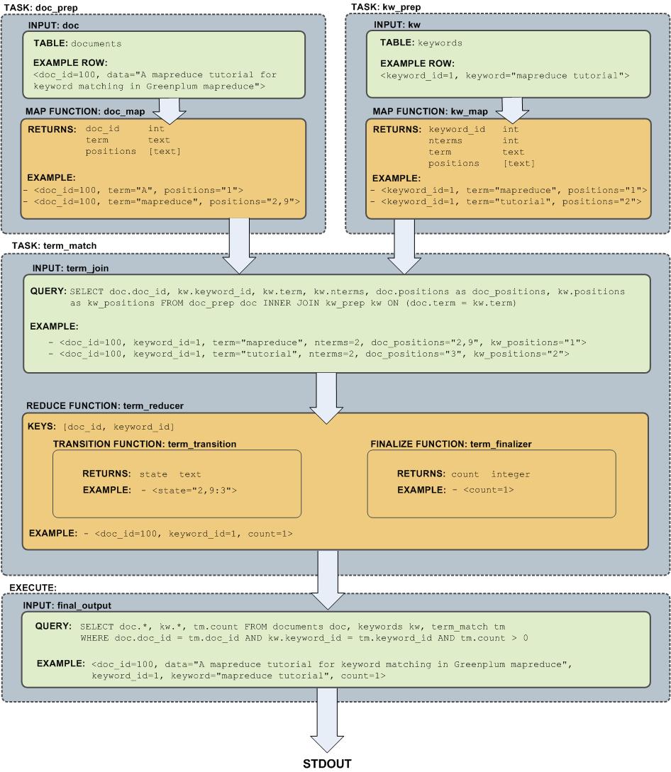
Query Performance
SynxDB dynamically eliminates irrelevant partitions in a table and optimally allocates memory for different operators in a query.These enhancements scan less data for a query, accelerate query processing, and support more concurrency.
-
Dynamic Partition Elimination
In SynxDB, values available only when a query runs are used to dynamically prune partitions, which improves query processing speed. Enable or deactivate dynamic partition elimination by setting the server configuration parameter
gp_dynamic_partition_pruningtoONorOFF; it isONby default. -
Memory Optimizations
SynxDB allocates memory optimally for different operators in a query and frees and re-allocates memory during the stages of processing a query.
Note SynxDB uses GPORCA, the SynxDB next generation query optimizer, by default. GPORCA extends the planning and optimization capabilities of the Postgres optimizer. For information about the features and limitations of GPORCA, see Overview of GPORCA.
Managing Spill Files Generated by Queries
SynxDB creates spill files, also known as workfiles, on disk if it does not have sufficient memory to run an SQL query in memory.
The maximum number of spill files for a given query is governed by the gp_workfile_limit_files_per_query server configuration parameter setting. The default value of 100,000 spill files is sufficient for the majority of queries.
If a query creates more than the configured number of spill files, SynxDB returns this error:
ERROR: number of workfiles per query limit exceeded
SynxDB may generate a large number of spill files when:
- Data skew is present in the queried data. To check for data skew, see Checking for Data Distribution Skew.
- The amount of memory allocated for the query is too low. You control the maximum amount of memory that can be used by a query with the SynxDB server configuration parameters max_statement_mem and statement_mem, or through resource group or resource queue configuration.
You might be able to run the query successfully by changing the query, changing the data distribution, or changing the system memory configuration. The gp_toolkit gp_workfile_* views display spill file usage information. You can use this information to troubleshoot and tune queries. The gp_workfile_* views are described in Checking Query Disk Spill Space Usage.
Additional documentation resources:
- Memory Consumption Parameters identifies the memory-related spill file server configuration parameters.
- Using Resource Groups describes memory and spill considerations when resource group-based resource management is active.
- Using Resource Queues describes memory and spill considerations when resource queue-based resource management is active.
Query Profiling
Examine the query plans of poorly performing queries to identify possible performance tuning opportunities.
SynxDB devises a query plan for each query. Choosing the right query plan to match the query and data structure is necessary for good performance. A query plan defines how SynxDB will run the query in the parallel execution environment.
The query optimizer uses data statistics maintained by the database to choose a query plan with the lowest possible cost. Cost is measured in disk I/O, shown as units of disk page fetches. The goal is to minimize the total execution cost for the plan.
View the plan for a given query with the EXPLAIN command. EXPLAIN shows the query optimizer’s estimated cost for the query plan. For example:
EXPLAIN SELECT * FROM names WHERE id=22;
EXPLAIN ANALYZE runs the statement in addition to displaying its plan. This is useful for determining how close the optimizer’s estimates are to reality. For example:
EXPLAIN ANALYZE SELECT * FROM names WHERE id=22;
Note In SynxDB, the default GPORCA optimizer co-exists with the Postgres Planner. The EXPLAIN output generated by GPORCA is different than the output generated by the Postgres Planner.
By default, SynxDB uses GPORCA to generate an execution plan for a query when possible.
When the EXPLAIN ANALYZE command uses GPORCA, the EXPLAIN plan shows only the number of partitions that are being eliminated. The scanned partitions are not shown. To show name of the scanned partitions in the segment logs set the server configuration parameter gp_log_dynamic_partition_pruning to on. This example SET command enables the parameter.
SET gp_log_dynamic_partition_pruning = on;
For information about GPORCA, see Querying Data.
Reading EXPLAIN Output
A query plan is a tree of nodes. Each node in the plan represents a single operation, such as a table scan, join, aggregation, or sort.
Read plans from the bottom to the top: each node feeds rows into the node directly above it. The bottom nodes of a plan are usually table scan operations: sequential, index, or bitmap index scans. If the query requires joins, aggregations, sorts, or other operations on the rows, there are additional nodes above the scan nodes to perform these operations. The topmost plan nodes are usually SynxDB motion nodes: redistribute, explicit redistribute, broadcast, or gather motions. These operations move rows between segment instances during query processing.
The output of EXPLAIN has one line for each node in the plan tree and shows the basic node type and the following execution cost estimates for that plan node:
-
cost —Measured in units of disk page fetches. 1.0 equals one sequential disk page read. The first estimate is the start-up cost of getting the first row and the second is the total cost of cost of getting all rows. The total cost assumes all rows will be retrieved, which is not always true; for example, if the query uses
LIMIT, not all rows are retrieved.Note The cost values generated by GPORCA and the Postgres Planner are not directly comparable. The two optimizers use different cost models, as well as different algorithms, to determine the cost of an execution plan. Nothing can or should be inferred by comparing cost values between the two optimizers.
In addition, the cost generated for any given optimizer is valid only for comparing plan alternatives for a given single query and set of statistics. Different queries can generate plans with different costs, even when keeping the optimizer a constant.
To summarize, the cost is essentially an internal number used by a given optimizer, and nothing should be inferred by examining only the cost value displayed in the
EXPLAINplans. -
rows —The total number of rows output by this plan node. This number is usually less than the number of rows processed or scanned by the plan node, reflecting the estimated selectivity of any
WHEREclause conditions. Ideally, the estimate for the topmost node approximates the number of rows that the query actually returns, updates, or deletes. -
width —The total bytes of all the rows that this plan node outputs.
Note the following:
- The cost of a node includes the cost of its child nodes. The topmost plan node has the estimated total execution cost for the plan. This is the number the optimizer intends to minimize.
- The cost reflects only the aspects of plan execution that the query optimizer takes into consideration. For example, the cost does not reflect time spent transmitting result rows to the client.
EXPLAIN Example
The following example describes how to read an EXPLAIN query plan for a query:
EXPLAIN SELECT * FROM names WHERE name = 'Joelle';
QUERY PLAN
------------------------------------------------------------
Gather Motion 2:1 (slice1) (cost=0.00..20.88 rows=1 width=13)
-> Seq Scan on 'names' (cost=0.00..20.88 rows=1 width=13)
Filter: name::text ~~ 'Joelle'::text
Read the plan from the bottom to the top. To start, the query optimizer sequentially scans the names table. Notice the WHERE clause is applied as a filter condition. This means the scan operation checks the condition for each row it scans and outputs only the rows that satisfy the condition.
The results of the scan operation are passed to a gather motion operation. In SynxDB, a gather motion is when segments send rows to the master. In this example, we have two segment instances that send to one master instance. This operation is working on slice1 of the parallel query execution plan. A query plan is divided into slices so the segments can work on portions of the query plan in parallel.
The estimated startup cost for this plan is 00.00 (no cost) and a total cost of 20.88 disk page fetches. The optimizer estimates this query will return one row.
Reading EXPLAIN ANALYZE Output
EXPLAIN ANALYZE plans and runs the statement. The EXPLAIN ANALYZE plan shows the actual execution cost along with the optimizer’s estimates. This allows you to see if the optimizer’s estimates are close to reality. EXPLAIN ANALYZE also shows the following:
-
The total runtime (in milliseconds) in which the query ran.
-
The memory used by each slice of the query plan, as well as the memory reserved for the whole query statement.
-
The number of workers (segments) involved in a plan node operation. Only segments that return rows are counted.
-
The maximum number of rows returned by the segment that produced the most rows for the operation. If multiple segments produce an equal number of rows,
EXPLAIN ANALYZEshows the segment with the longest <time> to end. -
The segment id of the segment that produced the most rows for an operation.
-
For relevant operations, the amount of memory (
work_mem) used by the operation. If thework_memwas insufficient to perform the operation in memory, the plan shows the amount of data spilled to disk for the lowest-performing segment. For example:Work_mem used: 64K bytes avg, 64K bytes max (seg0). Work_mem wanted: 90K bytes avg, 90K byes max (seg0) to lessen workfile I/O affecting 2 workers. -
The time (in milliseconds) in which the segment that produced the most rows retrieved the first row, and the time taken for that segment to retrieve all rows. The result may omit <time> to first row if it is the same as the <time> to end.
EXPLAIN ANALYZE Examples
This example describes how to read an EXPLAIN ANALYZE query plan using the same query. The bold parts of the plan show actual timing and rows returned for each plan node, as well as memory and time statistics for the whole query.
EXPLAIN ANALYZE SELECT * FROM names WHERE name = 'Joelle';
QUERY PLAN
------------------------------------------------------------
Gather Motion 2:1 (slice1; segments: 2) (cost=0.00..20.88 rows=1 width=13)
Rows out: 1 rows at destination with 0.305 ms to first row, 0.537 ms to end, start offset by 0.289 ms.
-> Seq Scan on names (cost=0.00..20.88 rows=1 width=13)
Rows out: Avg 1 rows x 2 workers. Max 1 rows (seg0) with 0.255 ms to first row, 0.486 ms to end, start offset by 0.968 ms.
Filter: name = 'Joelle'::text
Slice statistics:
(slice0) Executor memory: 135K bytes.
(slice1) Executor memory: 151K bytes avg x 2 workers, 151K bytes max (seg0).
Statement statistics:
Memory used: 128000K bytes
Total runtime: 22.548 ms
Read the plan from the bottom to the top. The total elapsed time to run this query was 22.548 milliseconds.
The sequential scan operation had only one segment (seg0) that returned rows, and it returned just 1 row. It took 0.255 milliseconds to find the first row and 0.486 to scan all rows. This result is close to the optimizer’s estimate: the query optimizer estimated it would return one row for this query. The gather motion (segments sending data to the master) received 1 row . The total elapsed time for this operation was 0.537 milliseconds.
Determining the Query Optimizer
You can view EXPLAIN output to determine if GPORCA is enabled for the query plan and whether GPORCA or the Postgres Planner generated the explain plan. The information appears at the end of the EXPLAIN output. The Settings line displays the setting of the server configuration parameter OPTIMIZER. The Optimizer status line displays whether GPORCA or the Postgres Planner generated the explain plan.
For these two example query plans, GPORCA is enabled, the server configuration parameter OPTIMIZER is on. For the first plan, GPORCA generated the EXPLAIN plan. For the second plan, SynxDB fell back to the Postgres Planner to generate the query plan.
QUERY PLAN
------------------------------------------------------------------------------------
Aggregate (cost=0.00..296.14 rows=1 width=8)
-> Gather Motion 2:1 (slice1; segments: 2) (cost=0.00..295.10 rows=1 width=8)
-> Aggregate (cost=0.00..294.10 rows=1 width=8)
-> Seq Scan on part (cost=0.00..97.69 rows=100040 width=1)
Settings: optimizer=on
Optimizer status: Pivotal Optimizer (GPORCA) version 1.584
(5 rows)
explain select count(*) from part;
QUERY PLAN
----------------------------------------------------------------------------------------
Aggregate (cost=3519.05..3519.06 rows=1 width=8)
-> Gather Motion 2:1 (slice1; segments: 2) (cost=3518.99..3519.03 rows=1 width=8)
-> Aggregate (cost=3518.99..3519.00 rows=1 width=8)
-> Seq Scan on part (cost=0.00..3018.79 rows=100040 width=1)
Settings: optimizer=on
Optimizer status: Postgres query optimizer
(5 rows)
For this query, the server configuration parameter OPTIMIZER is off.
explain select count(*) from part;
QUERY PLAN
----------------------------------------------------------------------------------------
Aggregate (cost=3519.05..3519.06 rows=1 width=8)
-> Gather Motion 2:1 (slice1; segments: 2) (cost=3518.99..3519.03 rows=1 width=8)
-> Aggregate (cost=3518.99..3519.00 rows=1 width=8)
-> Seq Scan on part (cost=0.00..3018.79 rows=100040 width=1)
Settings: optimizer=off
Optimizer status: Postgres query optimizer
(5 rows)
Examining Query Plans to Solve Problems
If a query performs poorly, examine its query plan and ask the following questions:
-
Do operations in the plan take an exceptionally long time? Look for an operation consumes the majority of query processing time. For example, if an index scan takes longer than expected, the index could be out-of-date and need to be reindexed. Or, adjust
enable_<operator>parameters to see if you can force the Postgres Planner to choose a different plan by deactivating a particular query plan operator for that query. -
Does the query planning time exceed query execution time? When the query involves many table joins, the Postgres Planner uses a dynamic algorithm to plan the query that is in part based on the number of table joins. You can reduce the amount of time that the Postgres Planner spends planning the query by setting the
join_collapse_limitandfrom_collapse_limitserver configuration parameters to a smaller value, such as8. Note that while smaller values reduce planning time, they may also yield inferior query plans. -
Are the optimizer’s estimates close to reality? Run
EXPLAIN ANALYZEand see if the number of rows the optimizer estimates is close to the number of rows the query operation actually returns. If there is a large discrepancy, collect more statistics on the relevant columns.See the SynxDB Reference Guide for more information on the
EXPLAIN ANALYZEandANALYZEcommands. -
Are selective predicates applied early in the plan? Apply the most selective filters early in the plan so fewer rows move up the plan tree. If the query plan does not correctly estimate query predicate selectivity, collect more statistics on the relevant columns. See the
ANALYZEcommand in the SynxDB Reference Guide for more information collecting statistics.You can also try reordering theWHEREclause of your SQL statement. -
Does the optimizer choose the best join order? When you have a query that joins multiple tables, make sure that the optimizer chooses the most selective join order. Joins that eliminate the largest number of rows should be done earlier in the plan so fewer rows move up the plan tree.
If the plan is not choosing the optimal join order, set
join_collapse_limit=1and use explicitJOINsyntax in your SQL statement to force the Postgres Planner to the specified join order. You can also collect more statistics on the relevant join columns.See the
ANALYZEcommand in the SynxDB Reference Guide for more information collecting statistics. -
Does the optimizer selectively scan partitioned tables? If you use table partitioning, is the optimizer selectively scanning only the child tables required to satisfy the query predicates? Scans of the parent tables should return 0 rows since the parent tables do not contain any data. See Verifying Your Partition Strategy for an example of a query plan that shows a selective partition scan.
-
Does the optimizer choose hash aggregate and hash join operations where applicable? Hash operations are typically much faster than other types of joins or aggregations. Row comparison and sorting is done in memory rather than reading/writing from disk. To enable the query optimizer to choose hash operations, there must be sufficient memory available to hold the estimated number of rows. Try increasing work memory to improve performance for a query. If possible, run an
EXPLAIN ANALYZEfor the query to show which plan operations spilled to disk, how much work memory they used, and how much memory was required to avoid spilling to disk. For example:Work_mem used: 23430K bytes avg, 23430K bytes max (seg0). Work_mem wanted: 33649K bytes avg, 33649K bytes max (seg0) to lessen workfile I/O affecting 2 workers.The “bytes wanted” message from
EXPLAIN ANALYZEis based on the amount of data written to work files and is not exact. The minimumwork_memneeded can differ from the suggested value.
Overview of SynxDB Integrated Analytics
SynxDB offers a unique combination of a powerful, massively parallel processing (MPP) database and advanced data analytics. This combination creates an ideal framework for data scientists, data architects and business decision makers to explore artificial intelligence (AI), machine learning, deep learning, text analytics, and geospatial analytics.
The SynxDB Integrated Analytics Ecosystem
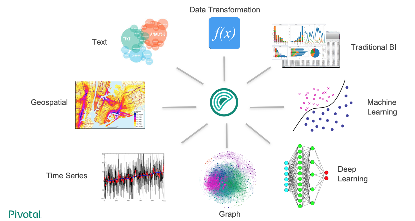
The following SynxDB analytics extensions are explored in different documentation sections, with installation and usage instructions:
Machine Learning and Deep Learning
The Apache MADlib extension allows SynxDB users to run different machine learning and deep learning functions, including feature engineering, model training, evaluation and scoring.
Geospatial Analytics
PostGIS is a spatial database extension for PostgreSQL that allows GIS (Geographic Information Systems) objects to be stored in the database. The SynxDB PostGIS extension includes support for GiST-based R-Tree spatial indexes and functions for analysis and processing of GIS objects.
Text Analytics
Text Analytics and Search enables processing of mass quantities of raw text data (such as social media feeds or e-mail databases) into mission-critical information that guides project and business decisions.
Programming Language Extensions
SynxDB supports a variety of procedural languages that you can use for programming database analytics. Refer to the linked documentation for installation and usage instructions.
Why SynxDB in Integrated Analytics
The importance of advanced analytics in its various forms is growing rapidly in enterprise computing. Key enterprise data typically resides in relational and document form and it is inefficient to copy data between systems to perform analytical operations. SynxDB is able to run both traditional and advanced analytics workloads in-database. This integrated capability greatly reduces the cost and the silos created by procuring and maintaining multiple tools and libraries.
SynxDB advanced analytics can be used to address a wide variety of problems in many verticals including automotive, finance, manufacturing, energy, government, education, telecommunications, on-line and traditional retail.
The SynxDB analytics capabilities allow you to:
- Analyze a multitude of data types – structured, text, geospatial, and graph – in a single environment, which can scale to petabytes and run algorithms designed for parallelism.
- Leverage existing SQL knowledge: SynxDB can run dozens of statistical, machine learning, and graph methods, via SQL.
- Train more models in less time by taking advantage of the parallelism in the MPP architecture and in-database analytics.
- Access the data where it lives, therefore integrate data and analytics in one place. SynxDB is infrastructure-agnostic and runs on bare metal, private cloud, and public cloud deployments.
- Use a multitude of data extensions. SynxDB supports Apache Kafka integration, extensions for HDFS, Hive, and HBase as well as reading/writing data from/to cloud storage, including Amazon S3 objects. Review the capabilities of the SynxDB Platform Extension Framework (PXF), which provides connectors that enable you to access data stored in sources external to your SynxDB deployment.
- Use familiar and leading BI and advanced analytics software that are ODBC/JDBC compatible, or have native integrations, including SAS, IBM Cognos, SAP Analytics Solutions, Qlik, Tableau, Apache Zeppelin, and Jupyter.
- Run deep learning algorithms using popular frameworks like Keras and TensorFlow in an MPP relational database, with GPU (Graphical Processing Unit) acceleration.
- Use containers capable of isolating executors from the host OS. SynxDB PL/Container implements a trusted language execution engine which permits customized data science workloads or environments created for different end user workloads.
- Use procedural languages to customize your analytics. SynxDB supports development in R, Python, Java, and other standard languages allowing you to distribute execution across the entire cluster to take advantage of the scale and parallelism.
Machine Learning and Deep Learning using MADlib
Apache MADlib is an open-source library for scalable in-database analytics. The SynxDB MADlib extension provides the ability to run machine learning and deep learning workloads in a SynxDB.
You can install it as an extension in a SynxDB system you can run data-parallel implementations of mathematical, statistical, graph, machine learning, and deep learning methods on structured and unstructured data. For SynxDB and MADlib version compatibility, refer to MADlib FAQ.
MADlib’s suite of SQL-based algorithms run at scale within a single SynxDB engine without needing to transfer data between the database and other tools.
MADlib is part of the database fabric with no changes to the SynxDB architecture. This makes it easy for database administrators to deploy and manage since it is not a separate daemon or separate software running outside the database.

Machine Learning
Apache MADlib consists of methods to support the full spectrum of data science activities. This includes data transformation and feature engineering, using methods in descriptive and inferential statistics, pivoting, sessionization and encoding categorical variables. There is also a comprehensive library of graph, supervised learning and unsupervised learning methods.
In the area of model selection, MADlib supports cross validation and the most common prediction metrics for evaluating the quality of predictions of a model. Please refer to the MADlib user guide for more information on these methods.
Deep Learning
Starting in Apache MADlib release 1.16, SynxDB supports using Keras and TensorFlow for deep learning. You can review the supported libraries and configuration instructions on the Apache MADlib pages as well as user documentation for Keras API using the Tensorflow backend. Note that it is not supported with RHEL 6.
MADlib supports Keras with a TensorFlow backend, with or without Graphics Processing Units (GPUs). GPUs can significantly accelerate the training of deep neural networks so they are typically used for enterprise level workloads. For further GPU information, visit the MADlib wiki, https://cwiki.apache.org/confluence/display/MADLIB/Deep+Learning.
PivotalR
MADlib can be used with PivotalR, an R client package that enables users to interact with data resident in the SynxDB. PivotalR can be considered as a wrapper around MADlib that translates R code into SQL to run on MPP databases and is designed for users familiar with R but with data sets that are too large for R.
The R language is an open-source language that is used for statistical computing. PivotalR is an R package that enables users to interact with data resident in SynxDB using the R client. Using PivotalR requires that MADlib is installed on the SynxDB.
PivotalR allows R users to leverage the scalability and performance of in-database analytics without leaving the R command line. The computational work is run in-database, while the end user benefits from the familiar R interface. Compared with respective native R functions, there is an increase in scalability and a decrease in running time. Furthermore, data movement, which can take hours for very large data sets, is eliminated with PivotalR.
Key features of the PivotalR package:
- Explore and manipulate data in the database with R syntax. SQL translation is performed by PivotalR.
- Use the familiar R syntax for predictive analytics algorithms, for example linear and logistic regression. PivotalR accesses the MADlib in-database analytics function calls.
- Comprehensive documentation package with examples in standard R format accessible from an R client.
- The PivotalR package also supports access to the MADlib functionality.
For information about PivotalR, including supported MADlib functionality, see https://cwiki.apache.org/confluence/display/MADLIB/PivotalR.
The archived packages for PivotalR can be found at https://cran.r-project.org/src/contrib/Archive/PivotalR/.
Prerequisites
Important SynxDB supports MADlib version 2.x for SynxDB 2 on RHEL8 platforms only. Upgrading from MADlib version 1.x to version 2.x is not supported.
MADlib requires the m4 macro processor version 1.4.13 or later. Ensure that you have access to, or superuser permissions to install, this package on each SynxDB host.
MADlib 2.x requires Python 3. If you are installing version 2.x, you must also set up the Python 3 environment by registering the python3u extension in all databases that will use MADlib:
CREATE EXTENSION python3u;
You must register the extension before you install MADlib 2.x.
Installing MADlib
To install MADlib on SynxDB, you first install a compatible SynxDB MADlib package and then install the MADlib function libraries on all databases that will use MADlib.
If you have GPUs installed on some or across all hosts in the cluster, then the segments residing on those hosts can benefit from GPU acceleration. GPUs and deep learning libraries such as Keras, TensorFlow, cudNN, and CUDA are managed separately from MADlib. For more information see the MADlib wiki instructions for deep learning and the MADlib user documentation for deep learning .
Installing the SynxDB MADlib Package
Before you install the MADlib package, make sure that your SynxDB is running, you have sourced synxdb_path.sh, and that the $MASTER_DATA_DIRECTORY and $GPHOME environment variables are set.
-
Download the MADlib extension package.
-
Copy the MADlib package to the SynxDB master host.
-
Unpack the MADlib distribution package. For example:
To unpack version 1.21:
$ tar xzvf madlib-1.21.0+1-gp6-rhel7-x86_64.tar.gzTo unpack version 2.1.0:
$ tar xzvf madlib-2.1.0-gp6-rhel8-x86_64.tar.gz -
Install the software package by running the
gppkgcommand. For example:To install version 1.21:
$ gppkg -i ./madlib-1.21.0+1-gp6-rhel7-x86_64/madlib-1.21.0+1-gp6-rhel7-x86_64.gppkgTo install version 2.1.0:
$ gppkg -i ./madlib-2.1.0-gp6-rhel8-x86_64/madlib-2.1.0-gp6-rhel8-x86_64.gppkg
Adding MADlib Functions to a Database
After installing the MADlib package, run the madpack command to add MADlib functions to SynxDB. madpack is in $GPHOME/madlib/bin.
$ madpack [-s <schema_name>] -p greenplum -c <user>@<host>:<port>/<database> install
For example, this command creates MADlib functions in the SynxDB testdb running on server mdw on port 5432. The madpack command logs in as the user gpadmin and prompts for password. The target schema is madlib.
$ madpack -s madlib -p greenplum -c gpadmin@mdw:5432/testdb install
After installing the functions, The SynxDB gpadmin superuser role should grant all privileges on the target schema (in the example madlib) to users who will be accessing MADlib functions. Users without access to the functions will get the error ERROR: permission denied for schema MADlib.
The madpack install-check option runs test using Madlib modules to check the MADlib installation:
$ madpack -s madlib -p greenplum -c gpadmin@mdw:5432/testdb install-check
Note The command
madpack -hdisplays information for the utility.
Upgrading MADlib
Important SynxDB does not support directly upgrading from MADlib 1.x to version 2.x. You must back up your MADlib models, uninstall version 1.x, install version 2.x, and reload the models.
You upgrade an installed MADlib version 1.x or 2.x package with the SynxDB gppkg utility and the MADlib madpack command.
For information about the upgrade paths that MADlib supports, see the MADlib support and upgrade matrix in the MADlib FAQ page.
Upgrading a MADlib 1.x Package
Important SynxDB does not support upgrading from MADlib version 1.x to version 2.x. Use this procedure to upgrade from an older MADlib version 1.x release to a newer version 1.x release.
To upgrade MADlib, run the gppkg utility with the -u option. This command upgrades an installed MADlib 1.x package to MADlib 1.21.0+1.
$ gppkg -u madlib-1.21.0+1-gp6-rhel7-x86_64.gppkg
Upgrading a MADlib 2.x Package
Important SynxDB does not support upgrading from MADlib version 1.x to version 2.x. Use this procedure to upgrade from an older MADlib version 2.x release to a newer version 2.x release.
To upgrade MADlib, run the gppkg utility with the -u option. This command upgrades an installed MADlib 2.0.x package to MADlib 2.1.0:
$ gppkg -u madlib-2.1.0-gp6-rhel8-x86_64.gppkg
Upgrading MADlib Functions
After you upgrade the MADlib package from one minor version to another, run madpack upgrade to upgrade the MADlib functions in a database schema.
Note Use
madpack upgradeonly if you upgraded a minor MADlib package version, for example from 1.19.0 to 1.21.0, or from 2.0.0 to 2.1.0. You do not need to update the functions within a patch version upgrade, for example from 1.16+1 to 1.16+3.
This example command upgrades the MADlib functions in the schema madlib of the SynxDB test.
madpack -s madlib -p greenplum -c gpadmin@mdw:5432/testdb upgrade
Uninstalling MADlib
When you remove MADlib support from a database, routines that you created in the database that use MADlib functionality will no longer work.
Remove MADlib objects from the database
Use the madpack uninstall command to remove MADlib objects from a SynxDB. For example, this command removes MADlib objects from the database testdb.
$ madpack -s madlib -p greenplum -c gpadmin@mdw:5432/testdb uninstall
Uninstall the SynxDB MADlib Package
If no databases use the MADlib functions, use the SynxDB gppkg utility with the -r option to uninstall the MADlib package. When removing the package you must specify the package and version. For example:
To uninstall MADlib package version 1.21.0:
$ gppkg -r madlib-1.21.0+1-gp6-rhel7-x86_64
To uninstall MADlib package version 2.1.0:
$ gppkg -r madlib-2.1.0-gp6-rhel8-x86_64
You can run the gppkg utility with the options -q --all to list the installed extensions and their versions.
After you uninstall the package, restart the database.
$ gpstop -r
Examples
Following are examples using the SynxDB MADlib extension:
See the MADlib documentation for additional examples.
Linear Regression
This example runs a linear regression on the table regr_example. The dependent variable data are in the y column and the independent variable data are in the x1 and x2 columns.
The following statements create the regr_example table and load some sample data:
DROP TABLE IF EXISTS regr_example;
CREATE TABLE regr_example (
id int,
y int,
x1 int,
x2 int
);
INSERT INTO regr_example VALUES
(1, 5, 2, 3),
(2, 10, 7, 2),
(3, 6, 4, 1),
(4, 8, 3, 4);
The MADlib linregr_train() function produces a regression model from an input table containing training data. The following SELECT statement runs a simple multivariate regression on the regr_example table and saves the model in the reg_example_model table.
SELECT madlib.linregr_train (
'regr_example', -- source table
'regr_example_model', -- output model table
'y', -- dependent variable
'ARRAY[1, x1, x2]' -- independent variables
);
The madlib.linregr_train() function can have additional arguments to set grouping columns and to calculate the heteroskedasticity of the model.
Note The intercept is computed by setting one of the independent variables to a constant
1, as shown in the preceding example.
Running this query against the regr_example table creates the regr_example_model table with one row of data:
SELECT * FROM regr_example_model;
-[ RECORD 1 ]------------+------------------------
coef | {0.111111111111127,1.14814814814815,1.01851851851852}
r2 | 0.968612680477111
std_err | {1.49587911309236,0.207043331249903,0.346449758034495}
t_stats | {0.0742781352708591,5.54544858420156,2.93987366103776}
p_values | {0.952799748147436,0.113579771006374,0.208730790695278}
condition_no | 22.650203241881
num_rows_processed | 4
num_missing_rows_skipped | 0
variance_covariance | {{2.23765432098598,-0.257201646090342,-0.437242798353582},
{-0.257201646090342,0.042866941015057,0.0342935528120456},
{-0.437242798353582,0.0342935528120457,0.12002743484216}}
The model saved in the regr_example_model table can be used with the MADlib linear regression prediction function, madlib.linregr_predict(), to view the residuals:
SELECT regr_example.*,
madlib.linregr_predict ( ARRAY[1, x1, x2], m.coef ) as predict,
y - madlib.linregr_predict ( ARRAY[1, x1, x2], m.coef ) as residual
FROM regr_example, regr_example_model m;
id | y | x1 | x2 | predict | residual
----+----+----+----+------------------+--------------------
1 | 5 | 2 | 3 | 5.46296296296297 | -0.462962962962971
3 | 6 | 4 | 1 | 5.72222222222224 | 0.277777777777762
2 | 10 | 7 | 2 | 10.1851851851852 | -0.185185185185201
4 | 8 | 3 | 4 | 7.62962962962964 | 0.370370370370364
(4 rows)
Association Rules
This example demonstrates the association rules data mining technique on a transactional data set. Association rule mining is a technique for discovering relationships between variables in a large data set. This example considers items in a store that are commonly purchased together. In addition to market basket analysis, association rules are also used in bioinformatics, web analytics, and other fields.
The example analyzes purchase information for seven transactions that are stored in a table with the MADlib function MADlib.assoc_rules. The function assumes that the data is stored in two columns with a single item and transaction ID per row. Transactions with multiple items consist of multiple rows with one row per item.
These commands create the table.
DROP TABLE IF EXISTS test_data;
CREATE TABLE test_data (
trans_id INT,
product text
);
This INSERT command adds the data to the table.
INSERT INTO test_data VALUES
(1, 'beer'),
(1, 'diapers'),
(1, 'chips'),
(2, 'beer'),
(2, 'diapers'),
(3, 'beer'),
(3, 'diapers'),
(4, 'beer'),
(4, 'chips'),
(5, 'beer'),
(6, 'beer'),
(6, 'diapers'),
(6, 'chips'),
(7, 'beer'),
(7, 'diapers');
The MADlib function madlib.assoc_rules() analyzes the data and determines association rules with the following characteristics.
- A support value of at least .40. Support is the ratio of transactions that contain X to all transactions.
- A confidence value of at least .75. Confidence is the ratio of transactions that contain X to transactions that contain Y. One could view this metric as the conditional probability of X given Y.
This SELECT command determines association rules, creates the table assoc_rules, and adds the statistics to the table.
SELECT * FROM madlib.assoc_rules (
.40, -- support
.75, -- confidence
'trans_id', -- transaction column
'product', -- product purchased column
'test_data', -- table name
'public', -- schema name
false); -- display processing details
This is the output of the SELECT command. There are two rules that fit the characteristics.
output_schema | output_table | total_rules | total_time
--------------+--------------+-------------+-----------------
public | assoc_rules | 2 | 00:00:01.153283
(1 row)
To view the association rules, you can run this SELECT command.
SELECT pre, post, support FROM assoc_rules
ORDER BY support DESC;
This is the output. The pre and post columns are the itemsets of left and right hand sides of the association rule respectively.
pre | post | support
-----------+--------+-------------------
{diapers} | {beer} | 0.714285714285714
{chips} | {beer} | 0.428571428571429
(2 rows)
Based on the data, beer and diapers are often purchased together. To increase sales, you might consider placing beer and diapers closer together on the shelves.
Naive Bayes Classification
Naive Bayes analysis predicts the likelihood of an outcome of a class variable, or category, based on one or more independent variables, or attributes. The class variable is a non-numeric categorial variable, a variable that can have one of a limited number of values or categories. The class variable is represented with integers, each integer representing a category. For example, if the category can be one of “true”, “false”, or “unknown,” the values can be represented with the integers 1, 2, or 3.
The attributes can be of numeric types and non-numeric, categorical, types. The training function has two signatures – one for the case where all attributes are numeric and another for mixed numeric and categorical types. Additional arguments for the latter identify the attributes that should be handled as numeric values. The attributes are submitted to the training function in an array.
The MADlib Naive Bayes training functions produce a features probabilities table and a class priors table, which can be used with the prediction function to provide the probability of a class for the set of attributes.
Naive Bayes Example 1 - Simple All-numeric Attributes
In the first example, the class variable is either 1 or 2 and there are three integer attributes.
-
The following commands create the input table and load sample data.
DROP TABLE IF EXISTS class_example CASCADE; CREATE TABLE class_example ( id int, class int, attributes int[]); INSERT INTO class_example VALUES (1, 1, '{1, 2, 3}'), (2, 1, '{1, 4, 3}'), (3, 2, '{0, 2, 2}'), (4, 1, '{1, 2, 1}'), (5, 2, '{1, 2, 2}'), (6, 2, '{0, 1, 3}');Actual data in production scenarios is more extensive than this example data and yields better results. Accuracy of classification improves significantly with larger training data sets.
-
Train the model with the
create_nb_prepared_data_tables()function.SELECT * FROM madlib.create_nb_prepared_data_tables ( 'class_example', -- name of the training table 'class', -- name of the class (dependent) column 'attributes', -- name of the attributes column 3, -- the number of attributes 'example_feature_probs', -- name for the feature probabilities output table 'example_priors' -- name for the class priors output table ); -
Create a table with data to classify using the model.
DROP TABLE IF EXISTS class_example_topredict; CREATE TABLE class_example_topredict ( id int, attributes int[]); INSERT INTO class_example_topredict VALUES (1, '{1, 3, 2}'), (2, '{4, 2, 2}'), (3, '{2, 1, 1}'); -
Create a classification view using the feature probabilities, class priors, and
class_example_topredicttables.SELECT madlib.create_nb_probs_view ( 'example_feature_probs', -- feature probabilities output table 'example_priors', -- class priors output table 'class_example_topredict', -- table with data to classify 'id', -- name of the key column 'attributes', -- name of the attributes column 3, -- number of attributes 'example_classified' -- name of the view to create ); -
Display the classification results.
SELECT * FROM example_classified; key | class | nb_prob -----+-------+--------- 1 | 1 | 0.4 1 | 2 | 0.6 3 | 1 | 0.5 3 | 2 | 0.5 2 | 1 | 0.25 2 | 2 | 0.75 (6 rows)
Naive Bayes Example 2 – Weather and Outdoor Sports
This example calculates the probability that the user will play an outdoor sport, such as golf or tennis, based on weather conditions.
The table weather_example contains the example values.
The identification column for the table is day, an integer type.
The play column holds the dependent variable and has two classifications:
- 0 - No
- 1 - Yes
There are four attributes: outlook, temperature, humidity, and wind. These are categorical variables. The MADlib create_nb_classify_view() function expects the attributes to be provided as an array of INTEGER, NUMERIC, or FLOAT8 values, so the attributes for this example are encoded with integers as follows:
- outlook may be sunny (1), overcast (2), or rain (3).
- temperature may be hot (1), mild (2), or cool (3).
- humidity may be high (1) or normal (2).
- wind may be strong (1) or weak (2).
The following table shows the training data, before encoding the variables.
day | play | outlook | temperature | humidity | wind
-----+------+----------+-------------+----------+--------
2 | No | Sunny | Hot | High | Strong
4 | Yes | Rain | Mild | High | Weak
6 | No | Rain | Cool | Normal | Strong
8 | No | Sunny | Mild | High | Weak
10 | Yes | Rain | Mild | Normal | Weak
12 | Yes | Overcast | Mild | High | Strong
14 | No | Rain | Mild | High | Strong
1 | No | Sunny | Hot | High | Weak
3 | Yes | Overcast | Hot | High | Weak
5 | Yes | Rain | Cool | Normal | Weak
7 | Yes | Overcast | Cool | Normal | Strong
9 | Yes | Sunny | Cool | Normal | Weak
11 | Yes | Sunny | Mild | Normal | Strong
13 | Yes | Overcast | Hot | Normal | Weak
(14 rows)
-
Create the training table.
DROP TABLE IF EXISTS weather_example; CREATE TABLE weather_example ( day int, play int, attrs int[] ); INSERT INTO weather_example VALUES ( 2, 0, '{1,1,1,1}'), -- sunny, hot, high, strong ( 4, 1, '{3,2,1,2}'), -- rain, mild, high, weak ( 6, 0, '{3,3,2,1}'), -- rain, cool, normal, strong ( 8, 0, '{1,2,1,2}'), -- sunny, mild, high, weak (10, 1, '{3,2,2,2}'), -- rain, mild, normal, weak (12, 1, '{2,2,1,1}'), -- etc. (14, 0, '{3,2,1,1}'), ( 1, 0, '{1,1,1,2}'), ( 3, 1, '{2,1,1,2}'), ( 5, 1, '{3,3,2,2}'), ( 7, 1, '{2,3,2,1}'), ( 9, 1, '{1,3,2,2}'), (11, 1, '{1,2,2,1}'), (13, 1, '{2,1,2,2}'); -
Create the model from the training table.
SELECT madlib.create_nb_prepared_data_tables ( 'weather_example', -- training source table 'play', -- dependent class column 'attrs', -- attributes column 4, -- number of attributes 'weather_probs', -- feature probabilities output table 'weather_priors' -- class priors ); -
View the feature probabilities:
SELECT * FROM weather_probs; class | attr | value | cnt | attr_cnt -------+------+-------+-----+---------- 1 | 3 | 2 | 6 | 2 1 | 1 | 2 | 4 | 3 0 | 1 | 1 | 3 | 3 0 | 1 | 3 | 2 | 3 0 | 3 | 1 | 4 | 2 1 | 4 | 1 | 3 | 2 1 | 2 | 3 | 3 | 3 1 | 2 | 1 | 2 | 3 0 | 2 | 2 | 2 | 3 0 | 4 | 2 | 2 | 2 0 | 3 | 2 | 1 | 2 0 | 1 | 2 | 0 | 3 1 | 1 | 1 | 2 | 3 1 | 1 | 3 | 3 | 3 1 | 3 | 1 | 3 | 2 0 | 4 | 1 | 3 | 2 0 | 2 | 3 | 1 | 3 0 | 2 | 1 | 2 | 3 1 | 2 | 2 | 4 | 3 1 | 4 | 2 | 6 | 2 (20 rows) -
To classify a group of records with a model, first load the data into a table. In this example, the table
t1has four rows to classify.DROP TABLE IF EXISTS t1; CREATE TABLE t1 ( id integer, attributes integer[]); insert into t1 values (1, '{1, 2, 1, 1}'), (2, '{3, 3, 2, 1}'), (3, '{2, 1, 2, 2}'), (4, '{3, 1, 1, 2}'); -
Use the MADlib
create_nb_classify_view()function to classify the rows in the table.SELECT madlib.create_nb_classify_view ( 'weather_probs', -- feature probabilities table 'weather_priors', -- classPriorsName 't1', -- table containing values to classify 'id', -- key column 'attributes', -- attributes column 4, -- number of attributes 't1_out' -- output table name );The result is four rows, one for each record in the
t1table.SELECT * FROM t1_out ORDER BY key; key | nb_classification -----+------------------- 1 | {0} 2 | {1} 3 | {1} 4 | {0} (4 rows)
References
MADlib web site is at http://madlib.apache.org/.
MADlib documentation is at http://madlib.apache.org/documentation.html.
PivotalR is a first class R package that enables users to interact with data resident in SynxDB and MADLib using an R client.
Graph Analytics
Many modern business problems involve connections and relationships between entities, and are not solely based on discrete data. Graphs are powerful at representing complex interconnections, and graph data modeling is very effective and flexible when the number and depth of relationships increase exponentially.
The use cases for graph analytics are diverse: social networks, transportation routes, autonomous vehicles, cyber security, criminal networks, fraud detection, health research, epidemiology, and so forth.
This chapter contains the following information:
What is a Graph?
Graphs represent the interconnections between objects (vertices) and their relationships (edges). Example objects could be people, locations, cities, computers, or components on a circuit board. Example connections could be roads, circuits, cables, or interpersonal relationships. Edges can have directions and weights, for example the distance between towns.
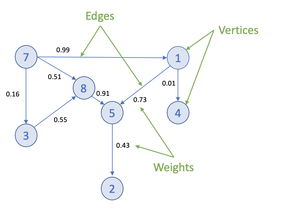
Graphs can be small and easily traversed - as with a small group of friends - or extremely large and complex, similar to contacts in a modern-day social network.
Graph Analytics on SynxDB
Efficient processing of very large graphs can be challenging. SynxDB offers a suitable environment for this work for these key reasons:
-
Using MADlib graph functions in SynxDB brings the graph computation close to where the data lives. Otherwise, large data sets need to be moved to a specialized graph database, requiring additional time and resources.
-
Specialized graph databases frequently use purpose-built languages. With SynxDB, you can invoke graph functions using the familiar SQL interface. For example, for the PageRank graph algorithm:
SELECT madlib.pagerank('vertex', -- Vertex table 'id', -- Vertex id column 'edge', -- Edge table 'src=src, dest=dest', -- Comma delimited string of edge arguments 'pagerank_out', -- Output table of PageRank 0.5); -- Damping factor SELECT * FROM pagerank_out ORDER BY pagerank DESC; -
A lot of data science problems are solved using a combination of models, with graphs being just one. Regression, clustering, and other methods available in SynxDB, make for a powerful combination.
-
SynxDB offers great benefits of scale, taking advantage of years of query execution and optimization research focused on large data sets.
Using Graph
Installing Graph Modules
To use the MADlib graph modules, install the version of MADlib corresponding to your SynxDB version. For SynxDB 2, see Installing MADlib.
Graph modules on MADlib support many algorithms.
Creating a Graph in SynxDB
To represent a graph in SynxDB, create tables that represent the vertices, edges, and their properties.
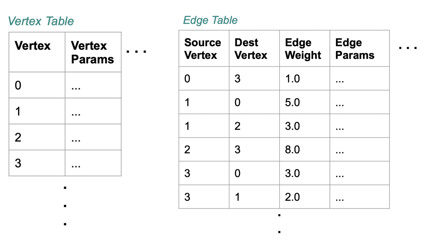
Using SQL, create the relevant tables in the database you want to use. This example uses testdb:
gpadmin@mdw ~]$ psql
dev=# \c testdb
Create a table for vertices, called vertex, and a table for edges and their weights, called edge:
testdb=# DROP TABLE IF EXISTS vertex, edge;
testdb=# CREATE TABLE vertex(id INTEGER);
testdb=# CREATE TABLE edge(
src INTEGER,
dest INTEGER,
weight FLOAT8
);
Insert values related to your specific use case. For example :
testdb#=> INSERT INTO vertex VALUES
(0),
(1),
(2),
(3),
(4),
(5),
(6),
(7);
testdb#=> INSERT INTO edge VALUES
(0, 1, 1.0),
(0, 2, 1.0),
(0, 4, 10.0),
(1, 2, 2.0),
(1, 3, 10.0),
(2, 3, 1.0),
(2, 5, 1.0),
(2, 6, 3.0),
(3, 0, 1.0),
(4, 0, -2.0),
(5, 6, 1.0),
(6, 7, 1.0);
Now select the Graph Module that suits your analysis.
Graph Modules
This section lists the graph functions supported in MADlib. They include: All Pairs Shortest Path (APSP), Breadth-First Search, Hyperlink-Induced Topic Search (HITS), PageRank and Personalized PageRank, Single Source Shortest Path (SSSP), Weakly Connected Components, and Measures. Explore each algorithm using the example edge and vertex tables already created.
All Pairs Shortest Path (APSP)
The all pairs shortest paths (APSP) algorithm finds the length (summed weights) of the shortest paths between all pairs of vertices, such that the sum of the weights of the path edges is minimized.
The function is:
graph_apsp( vertex_table,
vertex_id,
edge_table,
edge_args,
out_table,
grouping_cols
)
For details on the parameters, with examples, see the All Pairs Shortest Path in the Apache MADlib documentation.
Breadth-First Search
Given a graph and a source vertex, the breadth-first search (BFS) algorithm finds all nodes reachable from the source vertex by searching / traversing the graph in a breadth-first manner.
The function is:
graph_bfs( vertex_table,
vertex_id,
edge_table,
edge_args,
source_vertex,
out_table,
max_distance,
directed,
grouping_cols
)
For details on the parameters, with examples, see the Breadth-First Search in the Apache MADlib documentation.
Hyperlink-Induced Topic Search (HITS)
The all pairs shortest paths (APSP) algorithm finds the length (summed weights) of the shortest paths between all pairs of vertices, such that the sum of the weights of the path edges is minimized.
The function is:
graph_apsp( vertex_table,
vertex_id,
edge_table,
edge_args,
out_table,
grouping_cols
)
For details on the parameters, with examples, see the Hyperlink-Induced Topic Search in the Apache MADlib documentation.
PageRank and Personalized PageRank
Given a graph, the PageRank algorithm outputs a probability distribution representing a person’s likelihood to arrive at any particular vertex while randomly traversing the graph.
MADlib graph also includes a personalized PageRank, where a notion of importance provides personalization to a query. For example, importance scores can be biased according to a specified set of graph vertices that are of interest or special in some way.
The function is:
pagerank( vertex_table,
vertex_id,
edge_table,
edge_args,
out_table,
damping_factor,
max_iter,
threshold,
grouping_cols,
personalization_vertices
)
For details on the parameters, with examples, see the PageRank in the Apache MADlib documentation.
Single Source Shortest Path (SSSP)
Given a graph and a source vertex, the single source shortest path (SSSP) algorithm finds a path from the source vertex to every other vertex in the graph, such that the sum of the weights of the path edges is minimized.
The function is:
graph_sssp ( vertex_table,
vertex_id,
edge_table,
edge_args,
source_vertex,
out_table,
grouping_cols
)
For details on the parameters, with examples, see the Single Source Shortest Path in the Apache MADlib documentation.
Weakly Connected Components
Given a directed graph, a weakly connected component (WCC) is a subgraph of the original graph where all vertices are connected to each other by some path, ignoring the direction of edges.
The function is:
weakly_connected_components(
vertex_table,
vertex_id,
edge_table,
edge_args,
out_table,
grouping_cols
)
For details on the parameters, with examples, see the Weakly Connected Components in the Apache MADlib documentation.
Measures
These algorithms relate to metrics computed on a graph and include: Average Path Length, Closeness Centrality , Graph Diameter, and In-Out Degree.
Average Path Length
This function computes the shortest path average between pairs of vertices. Average path length is based on “reachable target vertices”, so it averages the path lengths in each connected component and ignores infinite-length paths between unconnected vertices. If the user requires the average path length of a particular component, the weakly connected components function may be used to isolate the relevant vertices.
The function is:
graph_avg_path_length( apsp_table,
output_table
)
This function uses a previously run APSP (All Pairs Shortest Path) output. For details on the parameters, with examples, see the Average Path Length in the Apache MADlib documentation.
Closeness Centrality
The closeness centrality algorithm helps quantify how much information passes through a given vertex. The function returns various closeness centrality measures and the k-degree for a given subset of vertices.
The function is:
graph_closeness( apsp_table,
output_table,
vertex_filter_expr
)
This function uses a previously run APSP (All Pairs Shortest Path) output. For details on the parameters, with examples, see the Closeness in the Apache MADlib documentation.
Graph Diameter
Graph diameter is defined as the longest of all shortest paths in a graph. The function is:
graph_diameter( apsp_table,
output_table
)
This function uses a previously run APSP (All Pairs Shortest Path) output. For details on the parameters, with examples, see the Graph Diameter in the Apache MADlib documentation.
In-Out Degree
This function computes the degree of each node. The node degree is the number of edges adjacent to that node. The node in-degree is the number of edges pointing in to the node and node out-degree is the number of edges pointing out of the node.
The function is:
graph_vertex_degrees( vertex_table,
vertex_id,
edge_table,
edge_args,
out_table,
grouping_cols
)
For details on the parameters, with examples, see the In-out Degree page in the Apache MADlib documentation.
References
MADlib on SynxDB is at Machine Learning and Deep Learning using MADlib.
MADlib Apache web site and MADlib release notes are at http://madlib.apache.org/.
MADlib user documentation is at http://madlib.apache.org/documentation.html.
Geospatial Analytics
This chapter contains the following information:
- About PostGIS
- SynxDB PostGIS Extension
- Enabling and Removing PostGIS Support
- Usage
- PostGIS Extension Support and Limitations
For information about upgrading PostGIS on SynxDB 2 systems, see Upgrading PostGIS 2.1.5 or 2.5.4
About PostGIS
PostGIS is a spatial database extension for PostgreSQL that allows GIS (Geographic Information Systems) objects to be stored in the database. The SynxDB PostGIS extension includes support for GiST-based R-Tree spatial indexes, and functions for analysis and processing of GIS objects.
The SynxDB PostGIS extension supports some PostGIS optional extensions and includes support for the PostGIS raster data type. With the PostGIS Raster objects, PostGIS geometry data type offers a single set of overlay SQL functions (such as ST_Intersects) operating seamlessly on vector and raster geospatial data. PostGIS Raster uses the GDAL (Geospatial Data Abstraction Library) translator library for raster geospatial data formats that presents a single raster abstract data model to a calling application.
For information about SynxDB PostGIS extension support, see PostGIS Extension Support and Limitations.
For information about PostGIS, see https://postgis.net/
For information about GDAL, see https://gdal.org/.
SynxDB PostGIS Extension
The SynxDB PostGIS extension is provided as a separate package. You can install the package using the SynxDB Package Manager (gppkg). For details, see gppkg in the SynxDB Utility Guide.
SynxDB supports the following PostGIS extension versions and components:
- PostGIS 2.5.4, and components Proj 4.8.0, Geos 3.10.2, GDAL 1.11.1, Json 0.12, Expat 2.4.4
- PostGIS 2.1.5, and components Proj 4.8.0, Geos 3.4.2, GDAL 1.11.1, Json 0.12, Expat 2.1.0
For information about the supported SynxDB extension packages and software versions, see Extensions in the SynxDB Tools and Extensions Compatibility topic.
There are significant changes in PostGIS 2.5.4 compared with 2.1.5. For a list of new and enhanced functions in PostGIS 2.5, see the PostGIS documentation PostGIS Functions new or enhanced in 2.5 and Release 2.5.4.
Note To upgrade PostGIS refer to Upgrading PostGIS 2.1.5 or 2.5.4.
This table lists the PostGIS extensions support by SynxDB PostGIS.
| PostGIS Extension | SynxDB PostGIS Notes |
|---|---|
postgisPostGIS and PostGIS Raster support |
Supported. Both PostGIS and PostGIS Raster are enabled when the SynxDB
postgis extension is enabled. |
postgis_tiger_geocoderThe US TIGER geocoder |
Supported. Installed with SynxDB PostGIS. Requires the
The US TIGER geocoder converts addresses (like a street address) to geographic coordinates. |
address_standardizerRule-based address standardizer |
Supported. Installed but not enabled with SynxDB PostGIS. Can be used with TIGER geocoder. A single line address parser that takes an input
address and normalizes it based on a set of rules stored in a table and helper
|
address_standardizer_data_usSample rules tables for US address data |
Supported. Installed but not enabled with SynxDB PostGIS. Can be used with the address standardizer. The extension contains |
fuzzystrmatchFuzzy string matching |
Supported. This extension is bundled but not enabled with SynxDB
Database. Required for the PostGIS TIGER geocoder. |
Note The PostGIS topology extension
postgis_topologyand the PostGIS 3D and geoprocessing extensionpostgis_sfcgalare not supported by SynxDB PostGIS and are not included in the SynxDB PostGIS extension package.
For information about the PostGIS extensions, see the PostGIS 2.5 documentation.
For information about SynxDB PostGIS feature support, see PostGIS Extension Support and Limitations.
Enabling and Removing PostGIS Support
This section describes how to enable and remove PostGIS and the supported PostGIS extensions, and how to configure PostGIS Raster.
- Enabling PostGIS Support
- Enabling GDAL Raster Drivers
- Enabling Out-of-Database Rasters
- Removing PostGIS Support
For information about upgrading PostGIS on SynxDB 2 systems, see Upgrading PostGIS 2.1.5 or 2.5.4
Enabling PostGIS Support
To enable PostGIS support, install the SynxDB PostGIS extension package into the SynxDB system, and then use the CREATE EXTENSION command to enable PostGIS support for an individual database.
Installing the SynxDB PostGIS Extension Package
Install SynxDB PostGIS extension package with the gppkg utility. For example, this command installs the package for RHEL 7.
gppkg -i postgis-2.5.4+pivotal.2.build.1-gp6-rhel7-x86_64.gppkg
After installing the package, source the synxdb_path.sh file and restart SynxDB. This command restarts SynxDB.
gpstop -ra
Installing the SynxDB PostGIS extension package updates the SynxDB system, including installing the supported PostGIS extensions to the system and updating synxdb_path.sh file with these lines for PostGIS Raster support.
export GDAL_DATA=$GPHOME/share/gdal
export POSTGIS_ENABLE_OUTDB_RASTERS=0
export POSTGIS_GDAL_ENABLED_DRIVERS=DISABLE_ALL
Using the CREATE EXTENSION Command
These steps enable the PostGIS extension and the extensions that are used with PostGIS.
-
To enable PostGIS and PostGIS Raster in a database, run this command after logging into the database.
CREATE EXTENSION postgis ;To enable PostGIS and PostGIS Raster in a specific schema, create the schema, set the
search_pathto the PostGIS schema, and then enable thepostgisextension with theWITH SCHEMAclause.SHOW search_path ; -- display the current search_path CREATE SCHEMA <schema_name> ; SET search_path TO <schema_name> ; CREATE EXTENSION postgis WITH SCHEMA <schema_name> ;After enabling the extension, reset the
search_pathand include the PostGIS schema in thesearch_pathif needed. -
If needed, enable the PostGIS TIGER geocoder after enabling the
postgisextension.To enable the PostGIS TIGER geocoder, you must enable the
fuzzystrmatchextension before enablingpostgis_tiger_geocoder. These two commands enable the extensions.CREATE EXTENSION fuzzystrmatch ; CREATE EXTENSION postgis_tiger_geocoder ; -
If needed, enable the rules-based address standardizer and add rules tables for the standardizer. These commands enable the extensions.
CREATE EXTENSION address_standardizer ; CREATE EXTENSION address_standardizer_data_us ;
Enabling GDAL Raster Drivers
PostGIS uses GDAL raster drivers when processing raster data with commands such as ST_AsJPEG(). As the default, PostGIS deactivates all raster drivers. You enable raster drivers by setting the value of the POSTGIS_GDAL_ENABLED_DRIVERS environment variable in the synxdb_path.sh file on all SynxDB hosts.
Alternatively, you can do it at the session level by setting postgis.gdal_enabled_drivers. For a SynxDB session, this example SET command enables three GDAL raster drivers.
SET postgis.gdal_enabled_drivers TO 'GTiff PNG JPEG';
This SET command sets the enabled drivers to the default for a session.
SET postgis.gdal_enabled_drivers = default;
To see the list of supported GDAL raster drivers for a SynxDB system, run the raster2pgsql utility with the -G option on the SynxDB master.
raster2pgsql -G
The command lists the driver long format name. The GDAL Raster table at https://gdal.org/drivers/raster/index.html lists the long format names and the corresponding codes that you specify as the value of the environment variable. For example, the code for the long name Portable Network Graphics is PNG. This example export line enables four GDAL raster drivers.
export POSTGIS_GDAL_ENABLED_DRIVERS="GTiff PNG JPEG GIF"
The gpstop -r command restarts the SynxDB system to use the updated settings in the synxdb_path.sh file.
After you have updated the synxdb_path.sh file on all hosts, and have restarted the SynxDB system, you can display the enabled raster drivers with the ST_GDALDrivers() function. This SELECT command lists the enabled raster drivers.
SELECT short_name, long_name FROM ST_GDALDrivers();
Enabling Out-of-Database Rasters
After installing PostGIS, the default setting POSTGIS_ENABLE_OUTDB_RASTERS=0 in the synxdb_path.sh file deactivates support for out-of-database rasters. To enable this feature, you can set the value to true (a non-zero value) on all hosts and restart the SynxDB system.
You can also activate or deactivate this feature for a SynxDB session. For example, this SET command enables the feature for the current session.
SET postgis.enable_outdb_rasters = true;
Note When the feature is enabled, the server configuration parameter
postgis.gdal_enabled_driversdetermines the accessible raster formats.
Removing PostGIS Support
You use the DROP EXTENSION command to remove support for the PostGIS extension and the extensions that are used with PostGIS.
Removing PostGIS support from a database does not remove these PostGIS Raster environment variables from the synxdb_path.sh file: GDAL_DATA, POSTGIS_ENABLE_OUTDB_RASTERS, POSTGIS_GDAL_ENABLED_DRIVERS. The environment variables are removed when you uninstall the PostGIS extension package.
Caution Removing PostGIS support from a database drops PostGIS database objects from the database without warning. Users accessing PostGIS objects might interfere with the dropping of PostGIS objects. See Notes.
Using the DROP EXTENSION Command
Depending on the extensions you enabled for PostGIS, drop support for the extensions in the database.
-
If you enabled the address standardizer and sample rules tables, these commands drop support for those extensions from the current database.
DROP EXTENSION IF EXISTS address_standardizer_data_us; DROP EXTENSION IF EXISTS address_standardizer; -
If you enabled the TIGER geocoder and the
fuzzystrmatchextension to use the TIGER geocoder, these commands drop support for those extensions.DROP EXTENSION IF EXISTS postgis_tiger_geocoder; DROP EXTENSION IF EXISTS fuzzystrmatch; -
Drop support for PostGIS and PostGIS Raster. This command drops support for those extensions.
DROP EXTENSION IF EXISTS postgis;If you enabled support for PostGIS and specified a specific schema with the
CREATE EXTENSIONcommand, you can update thesearch_pathand drop the PostGIS schema if required.
Uninstalling the SynxDB PostGIS Extension Package
After PostGIS support has been removed from all databases in the SynxDB system, you can remove the PostGIS extension package. For example, this gppkg command removes the PostGIS extension package.
gppkg -r postgis-2.5.4+pivotal.2
After removing the package, ensure that these lines for PostGIS Raster support are removed from the synxdb_path.sh file.
export GDAL_DATA=$GPHOME/share/gdal
export POSTGIS_ENABLE_OUTDB_RASTERS=0
export POSTGIS_GDAL_ENABLED_DRIVERS=DISABLE_ALL
Source the synxdb_path.sh file and restart SynxDB. This command restarts SynxDB.
gpstop -ra
Notes
Removing PostGIS support from a database drops PostGIS objects from the database. Dropping the PostGIS objects cascades to objects that reference the PostGIS objects. Before removing PostGIS support, ensure that no users are accessing the database. Users accessing PostGIS objects might interfere with dropping PostGIS objects.
For example, this CREATE TABLE command creates a table with column b that is defined with the PostGIS geometry data type.
# CREATE TABLE test(a int, b geometry) DISTRIBUTED RANDOMLY;
This is the table definition in a database with PostGIS enabled.
# \d test
Table "public.test"
Column | Type | Modifiers
--------+----------+-----------
a | integer |
b | geometry |
Distributed randomly
This is the table definition in a database after PostGIS support has been removed.
# \d test
Table "public.test"
Column | Type | Modifiers
--------+---------+-----------
a | integer |
Distributed randomly
Usage
The following example SQL statements create non-OpenGIS tables and geometries.
CREATE TABLE geom_test ( gid int4, geom geometry,
name varchar(25) );
INSERT INTO geom_test ( gid, geom, name )
VALUES ( 1, 'POLYGON((0 0 0,0 5 0,5 5 0,5 0 0,0 0 0))', '3D Square');
INSERT INTO geom_test ( gid, geom, name )
VALUES ( 2, 'LINESTRING(1 1 1,5 5 5,7 7 5)', '3D Line' );
INSERT INTO geom_test ( gid, geom, name )
VALUES ( 3, 'MULTIPOINT(3 4,8 9)', '2D Aggregate Point' );
SELECT * from geom_test WHERE geom &&
Box3D(ST_GeomFromEWKT('LINESTRING(2 2 0, 3 3 0)'));
The following example SQL statements create a table and add a geometry column to the table with a SRID integer value that references an entry in the SPATIAL_REF_SYS table. The INSERT statements add two geopoints to the table.
CREATE TABLE geotest (id INT4, name VARCHAR(32) );
SELECT AddGeometryColumn('geotest','geopoint', 4326,'POINT',2);
INSERT INTO geotest (id, name, geopoint)
VALUES (1, 'Olympia', ST_GeometryFromText('POINT(-122.90 46.97)', 4326));
INSERT INTO geotest (id, name, geopoint)
VALUES (2, 'Renton', ST_GeometryFromText('POINT(-122.22 47.50)', 4326));
SELECT name,ST_AsText(geopoint) FROM geotest;
Spatial Indexes
PostgreSQL provides support for GiST spatial indexing. The GiST scheme offers indexing even on large objects. It uses a system of lossy indexing in which smaller objects act as proxies for larger ones in the index. In the PostGIS indexing system, all objects use their bounding boxes as proxies in the index.
Building a Spatial Index
You can build a GiST index as follows:
CREATE INDEX indexname
ON tablename
USING GIST ( geometryfield );
PostGIS Extension Support and Limitations
This section describes SynxDB PostGIS extension feature support and limitations.
- Supported PostGIS Data Types
- Supported PostGIS Raster Data Types
- Supported PostGIS Index
- PostGIS Extension Limitations
In general, the SynxDB PostGIS extension does not support the following features:
- The PostGIS topology extension
postgis_topology - The PostGIS 3D and geoprocessing extension
postgis_sfcgal - A small number of user defined functions and aggregates
- PostGIS long transactions
For the PostGIS extensions supported by SynxDB PostGIS, see SynxDB PostGIS Extension.
Supported PostGIS Data Types
SynxDB PostGIS extension supports these PostGIS data types:
- box2d
- box3d
- geometry
- geography
For a list of PostGIS data types, operators, and functions, see the PostGIS reference documentation.
Supported PostGIS Raster Data Types
SynxDB PostGIS supports these PostGIS Raster data types.
- geomval
- addbandarg
- rastbandarg
- raster
- reclassarg
- summarystats
- unionarg
For information about PostGIS Raster data Management, queries, and applications, see https://postgis.net/docs/manual-2.5/using_raster_dataman.html.
For a list of PostGIS Raster data types, operators, and functions, see the PostGIS Raster reference documentation.
Supported PostGIS Index
SynxDB PostGIS extension supports the GiST (Generalized Search Tree) index.
PostGIS Extension Limitations
This section lists the SynxDB PostGIS extension limitations for user-defined functions (UDFs), data types, and aggregates.
-
Data types and functions related to PostGIS topology functionality, such as TopoGeometry, are not supported by SynxDB.
-
These PostGIS aggregates are not supported by SynxDB:
- ST_Collect
- ST_MakeLine
On a SynxDB with multiple segments, the aggregate might return different answers if it is called several times repeatedly.
-
SynxDB does not support PostGIS long transactions.
PostGIS relies on triggers and the PostGIS table
public.authorization_tablefor long transaction support. When PostGIS attempts to acquire locks for long transactions, SynxDB reports errors citing that the function cannot access the relation,authorization_table. -
SynxDB does not support type modifiers for user defined types.
The workaround is to use the
AddGeometryColumnfunction for PostGIS geometry. For example, a table with PostGIS geometry cannot be created with the following SQL command:CREATE TABLE geometries(id INTEGER, geom geometry(LINESTRING));Use the
AddGeometryColumnfunction to add PostGIS geometry to a table. For example, these following SQL statements create a table and add PostGIS geometry to the table:CREATE TABLE geometries(id INTEGER); SELECT AddGeometryColumn('public', 'geometries', 'geom', 0, 'LINESTRING', 2); -
The
_postgis_index_extentfunction is not supported on SynxDB 2 due to its dependence on spatial index operations. -
The
<->operator (geometry <-> geometry) returns the centroid/centroid distance for SynxDB 2. -
The TIGER geocoder extension is supported. However, upgrading the TIGER geocoder extension is not supported.
-
The
standardize_address()function useslex,gazorrulestables as parameters. If you are using tables apart fromus_lex,us_gazorus_rules, you should create them with the distribution policyDISTRIBUTED REPLICATEDto work for SynxDB.
Upgrading PostGIS 2.1.5 or 2.5.4
For SynxDB 2, you can upgrade from PostGIS 2.1.5 to 2.5.4, or from a PostGIS 2.5.4 package to a newer PostGIS 2.5.4 package.
- Upgrading from PostGIS 2.1.5 to the PostGIS 2.5.4 pivotal.3 (and later) Package
- Upgrade a PostGIS 2.5.4 Package from pivotal.1 or pivotal.2 to pivotal.3 (and later)
- Checking the PostGIS Version
Note For SynxDB 2, you can upgrade from PostGIS 2.1.5 to 2.5.4, or from a PostGIS 2.5.4 package to a newer PostGIS 2.5.4 package using the
postgis_manager.shscript described in the upgrade instructions.
Upgrading PostGIS using the postgis_manager.sh script does not require you to remove PostGIS support and re-enable it.
Removing PostGIS support from a database drops PostGIS database objects from the database without warning. Users accessing PostGIS objects might interfere with the dropping of PostGIS objects. See the Notes section in Removing PostGIS Support.
Upgrading from PostGIS 2.1.5 to the PostGIS 2.5.4 pivotal.3 (and later) Package
A PostGIS 2.5.4 pivotal.3 (and later) package contains PostGIS 2.5.4. Also, the PostGIS 2.5.4 pivotal.3 (and later) package supports using the CREATE EXTENSION command and the DROP EXTENSION command to enable and remove PostGIS support in a database. See Notes.
After upgrading the SynxDB PostGIS package, you can remove the PostGIS 2.1.5 package (gppkg) from the SynxDB system. See Removing the PostGIS 2.1.5 package.
-
Confirm you have a PostGIS 2.1.5 package such as
postgis-2.1.5+pivotal.1installed in a SynxDB system. See Checking the PostGIS Version. -
Install the PostGIS 2.5.4 package into the SynxDB system with the
gppkgutility.gppkg -i postgis-2.5.4+pivotal.3.build.1-gp6-rhel7-x86_64.gppkgRun the
gppkg -q --allcommand to verify the updated package version is installed in the SynxDB system. -
For all databases with PostGIS enabled, run the PostGIS 2.5.4
postgis_manager.shscript in the directory$GPHOME/share/postgresql/contrib/postgis-2.5to upgrade PostGIS in that database. This command upgrades PostGIS that is enabled in the databasemytestin the SynxDB system.$GPHOME/share/postgresql/contrib/postgis-2.5/postgis_manager.sh mytest upgrade -
After running the script, you can verify that PostGIS 2.5.4 is installed and enabled as an extension in a database with this query.
# SELECT * FROM pg_available_extensions WHERE name = 'postgis' ; -
You can validate that PostGIS 2.5 is enabled in the database with the
postgis_version()function.
After you have completed the upgrade to PostGIS 2.5.4 pivotal.3 or later for the SynxDB system and all the databases with PostGIS enabled, you enable PostGIS in a new database with the CREATE EXTENSION postgis command. To remove PostGIS support, use the DROP EXTENSION postgis CASCADE command.
Removing the PostGIS 2.1.5 package
After upgrading the databases in the SynxDB system, you can remove the PostGIS 2.1.5 package from the system. This command removes the postgis-2.1.5+pivotal.2 package from a SynxDB system.
gppkg -r postgis-2.1.5+pivotal.2
Run the gppkg -q --all command to list the installed SynxDB packages.
Upgrade a PostGIS 2.5.4 Package from pivotal.1 or pivotal.2 to pivotal.3 (or later)
You can upgrade the installed PostGIS 2.5.4 package from pivotal.1 or pivotal.2 to pivotal.3 or later (a minor release upgrade). The upgrade updates the PostGIS 2.5.4 package to the minor release (pivotal.3\ or later) that uses the same PostGIS version (2.5.4).
The pivotal.3 minor release and later support using the CREATE EXTENSION command and the DROP EXTENSION command to enable and remove PostGIS support in a database. See Notes.
-
Confirm you have a PostGIS 2.5.4 package
postgis-2.5.4+**pivotal.1**orpostgis-2.5.4+**pivotal.2**installed in a SynxDB system. See Checking the PostGIS Version. -
Upgrade the PostGIS package in the SynxDB system using the
gppkgoption-u. The following command updates the package to thepostgis-2.5.4+pivotal.3.build.1package.gppkg -u postgis-2.5.4+pivotal.3.build.1-gp6-rhel7-x86_64.gppkg -
Run the
gppkg -q --allcommand to verify the updated package version is installed in the SynxDB system. -
For all databases with PostGIS enabled, upgrade PostGIS with the PostGIS 2.5.4
postgis_manager.shscript that is in the directory$GPHOME/share/postgresql/contrib/postgis-2.5to upgrade PostGIS in that database. This command upgrades PostGIS that is enabled in the databasemytestin the SynxDB system.$GPHOME/share/postgresql/contrib/postgis-2.5/postgis_manager.sh mytest upgrade
After you have completed the upgrade to PostGIS 2.5.4 pivotal.3 or later for the SynxDB system and all the databases with PostGIS enabled, you enable PostGIS in a new database with the CREATE EXTENSION postgis command. To remove PostGIS support, use the DROP EXTENSION postgis CASCADE command.
Checking the PostGIS Version
When upgrading PostGIS you must check the version of the SynxDB PostGIS package installed on the SynxDB system and the version of PostGIS enabled in the database.
-
Check the installed PostGIS package version with the
gppkgutility. This command lists all installed SynxDB packages.gppkg -q --all -
Check the enabled PostGIS version in a database with the
postgis_version()function. Thispsqlcommand displays the version PostGIS that is enabled for the databasetestdb.psql -d testdb -c 'select postgis_version();'If PostGIS is not enabled for the database, SynxDB returns a
function does not existerror. -
For the SynxDB PostGIS package
postgis-2.5.4+pivotal.2and later, you can display the PostGIS extension version and state in a database with this query.# SELECT * FROM pg_available_extensions WHERE name = 'postgis' ;The query displays the version whether the extension is installed and enabled in a database. If the PostGIS package is not installed, no rows are returned.
Notes
Starting with the SynxDB postgis-2.5.4+pivotal.2 package, you enable support for PostGIS in a database with the CREATE EXTENSION command. For previous PostGIS 2.5.4 packages and all PostGIS 2.1.5 packages, you use an SQL script.
Text Analytics and Search
SynxDB text search is PostgreSQL text search ported to the SynxDB MPP platform. SynxDB text search is immediately available to you, with no need to install and maintain additional software. For full details on this topic, see SynxDB text search.
Procedural Languages
SynxDB supports a pluggable procedural language architecture by virtue of its PostgreSQL heritage. This allows user-defined functions to be written in languages other than SQL and C. It may be more convenient to develop analytics functions in a familiar procedural language compared to using only SQL constructs. For example, suppose you have existing Python code that you want to use on data in SynxDB, you can wrap this code in a PL/Python function and call it from SQL.
The available SynxDB procedural languages are typically packaged as extensions. You register a language in a database using the CREATE EXTENSION command. You remove a language from a database with DROP EXTENSION.
The SynxDB distribution supports the following procedural languages; refer to the linked language documentation for installation and usage instructions:
PL/Container Language
PL/Container enables users to run SynxDB procedural language functions inside a Docker container, to avoid security risks associated with running Python or R code on SynxDB segment hosts. For Python, PL/Container also enables you to use the Compute Unified Device Architecture (CUDA) API with NVIDIA GPU hardware in your procedural language functions. This topic covers information about the architecture, installation, and setup of PL/Container:
- About the PL/Container Language Extension
- Install PL/Container
- Upgrade PL/Container
- Uninstall PL/Container
- Docker References
For detailed information about using PL/Container, refer to:
The PL/Container language extension is available as an open source module. For information about the module, see the README file in the GitHub repository at https://github.com/greenplum-db/plcontainer-archive.
About the PL/Container Language Extension
The SynxDB PL/Container language extension allows you to create and run PL/Python or PL/R user-defined functions (UDFs) securely, inside a Docker container. Docker provides the ability to package and run an application in a loosely isolated environment called a container. For information about Docker, see the Docker web site.
Running UDFs inside the Docker container ensures that:
- The function execution process takes place in a separate environment and allows decoupling of the data processing. SQL operators such as “scan,” “filter,” and “project” are run at the query executor (QE) side, and advanced data analysis is run at the container side.
- User code cannot access the OS or the file system of the local host.
- User code cannot introduce any security risks.
- Functions cannot connect back to the SynxDB if the container is started with limited or no network access.
PL/Container Architecture
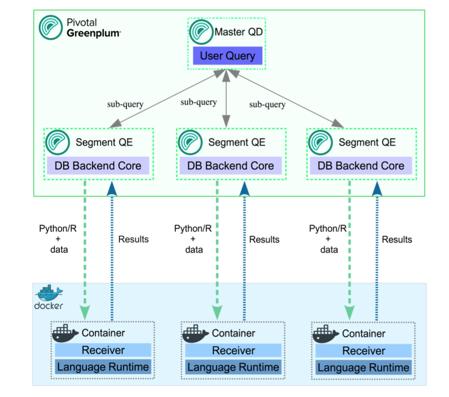
Example of the process flow:
Consider a query that selects table data using all available segments, and transforms the data using a PL/Container function. On the first call to a function in a segment container, the query executor on the master host starts the container on that segment host. It then contacts the running container to obtain the results. The container might respond with a Service Provider Interface (SPI) - a SQL query run by the container to get some data back from the database - returning the result to the query executor.
A container running in standby mode waits on the socket and does not consume any CPU resources. PL/Container memory consumption depends on the amount of data cached in global dictionaries.
The container connection is closed by closing the SynxDB session that started the container, and the container shuts down.
About PL/Container 3 Beta
Note PL/Container 3 Beta is deprecated and will be removed in a future SynxDB release.
SynxDB 2 includes PL/Container version 3 Beta, which:
- Reduces the number of processes created by PL/Container, in order to save system resources.
- Supports more containers running concurrently.
- Includes improved log messages to help diagnose problems.
- Supports the
DOcommand (anonymous code block).
PL/Container 3 is currently a Beta feature, and provides only a Beta R Docker image for running functions; Python images are not yet available. Save and uninstall any existing PL/Container software before you install PL/Container 3 Beta.
Install PL/Container
This topic includes how to:
- Install Docker
- Install PL/Container
- Install the PL/Container Docker images
- Test the PL/Container installation
The following sections describe these tasks in detail.
Prerequisites
-
For PL/Container 2.1.x use SynxDB 2 on CentOS 7.x (or later), RHEL 7.x (or later), or Ubuntu 18.04.
Note PL/Container 2.1.x supports Docker images with Python 3 installed.
-
For PL/Container 3 Beta use SynxDB 2 on CentOS 7.x (or later), RHEL 7.x (or later), or Ubuntu 18.04.
-
The minimum Linux OS kernel version supported is 3.10. To verify your kernel release use:
$ uname -r -
The minimum supported Docker versions on all hosts is Docker 19.03.
Install Docker
To use PL/Container you need to install Docker on all SynxDB host systems. These instructions show how to set up the Docker service on CentOS 7 but RHEL 7 is a similar process.
These steps install the docker package and start the Docker service as a user with sudo privileges.
-
Ensure the user has sudo privileges or is root.
-
Install the dependencies required for Docker:
sudo yum install -y yum-utils device-mapper-persistent-data lvm2 -
Add the Docker repo:
sudo yum-config-manager --add-repo https://download.docker.com/linux/centos/docker-ce.repo -
Update yum cache:
sudo yum makecache fast -
Install Docker:
sudo yum -y install docker-ce -
Start Docker daemon:
sudo systemctl start docker -
On each SynxDB host, the
gpadminuser should be part of the docker group for the user to be able to manage Docker images and containers. Assign the SynxDB administratorgpadminto the groupdocker:sudo usermod -aG docker gpadmin -
Exit the session and login again to update the privileges.
-
Configure Docker to start when the host system starts:
sudo systemctl enable docker.servicesudo systemctl start docker.service -
Run a Docker command to test the Docker installation. This command lists the currently running Docker containers.
docker ps -
After you install Docker on all SynxDB hosts, restart the SynxDB system to give SynxDB access to Docker.
gpstop -ra
For a list of observations while using Docker and PL/Container, see the Notes section. For a list of Docker reference documentation, see Docker References.
Install PL/Container
Install the PL/Container language extension using the gppkg utility.
-
Download the “PL/Container for RHEL 7” package that applies to your SynxDB version. PL/Container is listed under SynxDB Procedural Languages.
-
As
gpadmin, copy the PL/Container language extension package to the master host. -
Run the package installation command:
gppkg -i plcontainer-2.1.1-rhel7-x86_64.gppkg -
Source the file
$GPHOME/synxdb_path.sh:source $GPHOME/synxdb_path.sh -
Make sure SynxDB is up and running:
gpstate -sIf it’s not, start it:
gpstart -a -
For PL/Container version 3 Beta only, add the
plc_coordinatorshared library to the SynxDBshared_preload_librariesserver configuration parameter. Be sure to retain any previous setting of the parameter. For example:gpconfig -s shared_preload_libraries Values on all segments are consistent GUC : shared_preload_libraries Coordinator value: diskquota Segment value: diskquota gpconfig -c shared_preload_libraries -v 'diskquota,plc_coordinator' -
Restart SynxDB:
gpstop -ra -
Login into one of the available databases, for example:
psql postgres -
Register the PL/Container extension, which installs the
plcontainerutility:CREATE EXTENSION plcontainer;You’ll need to register the utility separately on each database that might need the PL/Container functionality.
Install PL/Container Docker Images
Install the Docker images that PL/Container will use to create language-specific containers to run the UDFs. Before installing, review this compatiblity matrix:
| plcontainer version | R image version | python2 image version | python3 image version |
|---|---|---|---|
| 2.3.2 | 2.1.3 | 2.1.3 | 2.3.2 |
| 2.4.0 | 2.1.3 | 2.1.3 | 2.4.0 |
Note: The PL/Container open source module contains dockerfiles to build Docker images that can be used with PL/Container. You can build a Docker image to run PL/Python UDFs and a Docker image to run PL/R UDFs. See the dockerfiles in the GitHub repository at https://github.com/greenplum-db/plcontainer-archive.
-
Download the files that contain the Docker images. For example, click on “PL/Container Image for Python 2.2.0” which downloads plcontainer-python3-image-2.2.0-gp6.tar.gz with Python 3.9 and the Python 3.9 Data Science Module Package.
If you require different images from the ones provided by SynxDB, you can create custom Docker images, install the image and add the image to the PL/ Container configuration.
-
If you are using PL/Container 3 Beta, note that this Beta version is compatible only with the associated
plcontainer-r-image-3.0.0-beta-gp6.tar.gzimage. -
Use the
plcontainer image-addcommand to install an image on all SynxDB hosts. Provide the-foption to specify the file system location of a downloaded image file. For example:# Install a Python 2 based Docker image plcontainer image-add -f /home/gpadmin/plcontainer-python-image-2.2.0-gp6.tar.gz # Install a Python 3 based Docker image plcontainer image-add -f /home/gpadmin/plcontainer-python3-image-2.2.0-gp6.tar.gz # Install an R based Docker image plcontainer image-add -f /home/gpadmin/plcontainer-r-image-2.1.3-gp6.tar.gz # Install the Beta R image for use with PL/Container 3.0.0 Beta plcontainer image-add -f /home/gpadmin/plcontainer-r-image-3.0.0-beta-gp6.tar.gzThe utility displays progress information, similar to:
20200127:21:54:43:004607 plcontainer:mdw:gpadmin-[INFO]:-Checking whether docker is installed on all hosts... 20200127:21:54:43:004607 plcontainer:mdw:gpadmin-[INFO]:-Distributing image file /home/gpadmin/plcontainer-python-images-1.5.0.tar to all hosts... 20200127:21:54:55:004607 plcontainer:mdw:gpadmin-[INFO]:-Loading image on all hosts... 20200127:21:55:37:004607 plcontainer:mdw:gpadmin-[INFO]:-Removing temporary image files on all hosts...By default, the
image-addcommand copies the image to each SynxDB segment and standby master host, and installs the image. When you specify the[-ulc | --use_local_copy]option,plcontainerinstalls the image only on the host on which you run the command. Use this option when the PL/Container image already resides on disk on a host.For more information on
image-addoptions, visit the plcontainer reference page. -
To display the installed Docker images on the local host use:
$ plcontainer image-listREPOSITORY TAG IMAGE ID CREATED pivotaldata/plcontainer_r_shared devel 7427f920669d 10 months ago pivotaldata/plcontainer_python_shared devel e36827eba53e 10 months ago pivotaldata/plcontainer_python3_shared devel y32827ebe55b 5 months ago -
Add the image information to the PL/Container configuration file using
plcontainer runtime-add, to allow PL/Container to associate containers with specified Docker images.Use the
-roption to specify your own user defined runtime ID name, use the-ioption to specify the Docker image, and the-loption to specify the Docker image language. When there are multiple versions of the same docker image, for example 1.0.0 or 1.2.0, specify the TAG version using “:” after the image name.# Add a Python 2 based runtime plcontainer runtime-add -r plc_python_shared -i pivotaldata/plcontainer_python_shared:devel -l python # Add a Python 3 based runtime that is supported with PL/Container 2.2.x plcontainer runtime-add -r plc_python3_shared -i pivotaldata/plcontainer_python3_shared:devel -l python3 # Add an R based runtime plcontainer runtime-add -r plc_r_shared -i pivotaldata/plcontainer_r_shared:devel -l rThe utility displays progress information as it updates the PL/Container configuration file on the SynxDB instances.
For details on other
runtime-addoptions, see the plcontainer reference page. -
Optional: Use SynxDB resource groups to manage and limit the total CPU and memory resources of containers in PL/Container runtimes. In this example, the Python runtime will be used with a preconfigured resource group 16391:
plcontainer runtime-add -r plc_python_shared -i pivotaldata/plcontainer_python_shared:devel -l python -s resource_group_id=16391For more information about enabling, configuring, and using SynxDB resource groups with PL/Container, see PL/Container Resource Management.
You can now create a simple function to test your PL/Container installation.
Test the PL/Container Installation
List the names of the runtimes your created and added to the PL/Container XML file:
plcontainer runtime-show
which will show a list of all installed runtimes:
PL/Container Runtime Configuration:
---------------------------------------------------------
Runtime ID: plc_python_shared
Linked Docker Image: pivotaldata/plcontainer_python_shared:devel
Runtime Setting(s):
Shared Directory:
---- Shared Directory From HOST '/usr/local/synxdb/./bin/plcontainer_clients' to Container '/clientdir', access mode is 'ro'
---------------------------------------------------------
You can also view the PL/Container configuration information with the plcontainer runtime-show -r <runtime_id> command. You can view the PL/Container configuration XML file with the plcontainer runtime-edit command.
Use the psql utility and select an existing database:
psql postgres;
If the PL/Container extension is not registered with the selected database, first enable it using:
postgres=# CREATE EXTENSION plcontainer;
Create a simple function to test your installation; in the example, the function will use the runtime plc_python_shared:
postgres=# CREATE FUNCTION dummyPython() RETURNS text AS $$
# container: plc_python_shared
return 'hello from Python'
$$ LANGUAGE plcontainer;
And test the function using:
postgres=# SELECT dummyPython();
dummypython
-------------------
hello from Python
(1 row)
Similarly, to test the R runtime:
postgres=# CREATE FUNCTION dummyR() RETURNS text AS $$
# container: plc_r_shared
return ('hello from R')
$$ LANGUAGE plcontainer;
CREATE FUNCTION
postgres=# select dummyR();
dummyr
--------------
hello from R
(1 row)
For further details and examples about using PL/Container functions, see PL/Container Functions.
Upgrade PL/Container
To upgrade PL/Container, you save the current configuration, upgrade PL/Container, and then restore the configuration after upgrade. There is no need to update the Docker images when you upgrade PL/Container.
Note Before you perform this upgrade procedure, ensure that you have migrated your PL/Container package from your previous SynxDB installation to your new SynxDB installation. Refer to the gppkg command for package installation and migration information.
Note You cannot upgrade to PL/Container 3 Beta. To install PL/Container 3 Beta, first save and then uninstall your existing PL/Container software. Then follow the instructions in Install PL/Container.
To upgrade, perform the following procedure:
-
Save the PL/Container configuration. For example, to save the configuration to a file named
plcontainer202-backup.xmlin the local directory:$ plcontainer runtime-backup -f plcontainer202-backup.xml -
Use the SynxDB
gppkgutility with the-uoption to update the PL/Container language extension. For example, the following command updates the PL/Container language extension to version 2.2.0 on a Linux system:$ gppkg -u plcontainer-2.2.0-gp6-rhel7_x86_64.gppkg -
Source the SynxDB environment file
$GPHOME/synxdb_path.sh.$ source $GPHOME/synxdb_path.sh -
Restore the PL/Container configuration that you saved in a previous step:
$ plcontainer runtime-restore -f plcontainer202-backup.xml -
Restart SynxDB.
$ gpstop -ra -
You do not need to re-register the PL/Container extension in the databases in which you previously created the extension but ensure that you register the PL/Container extension in each new database that will run PL/Container UDFs. For example, the following command registers PL/Container in a database named
mytest:$ psql -d mytest -c 'CREATE EXTENSION plcontainer;'The command also creates PL/Container-specific functions and views.
Uninstall PL/Container
To uninstall PL/Container, remove Docker containers and images, and then remove the PL/Container support from SynxDB.
When you remove support for PL/Container, the plcontainer user-defined functions that you created in the database will no longer work.
Uninstall Docker Containers and Images
On the SynxDB hosts, uninstall the Docker containers and images that are no longer required.
The plcontainer image-list command lists the Docker images that are installed on the local SynxDB host.
The plcontainer image-delete command deletes a specified Docker image from all SynxDB hosts.
Some Docker containers might exist on a host if the containers were not managed by PL/Container. You might need to remove the containers with Docker commands. These docker commands manage Docker containers and images on a local host.
- The command
docker ps -alists all containers on a host. The commanddocker stopstops a container. - The command
docker imageslists the images on a host. - The command
docker rmiremoves images. - The command
docker rmremoves containers.
Remove PL/Container Support for a Database
To remove support for PL/Container, drop the extension from the database. Use the psql utility with DROP EXTENSION command (using -c) to remove PL/Container from mytest database.
psql -d mytest -c 'DROP EXTENSION plcontainer CASCADE;'
The CASCADE keyword drops PL/Container-specific functions and views.
Remove PL/Container 3 Beta Shared Library
This step is required only if you have installed PL/Container 3 Beta. Before you remove the extension from your system with gppkg, remove the shared library configuration for the plc_coordinator process:
-
Examine the
shared_preload_librariesserver configuration parameter setting.$ gpconfig -s shared_preload_libraries-
If
plc_coordinatoris the only library listed, remove the configuration parameter setting:$ gpconfig -r shared_preload_librariesRemoving a server configuration parameter comments out the setting in the postgresql.conf file.
-
If there are multiple libraries listed, remove
plc_coordinatorfrom the list and re-set the configuration parameter. For example, ifshared_preload_librariesis set to'diskquota,plc_coordinator':$ gpconfig -c shared_preload_libraries -v 'diskquota'
-
-
Restart the SynxDB cluster:
$ gpstop -ra
Uninstall the PL/Container Language Extension
If no databases have plcontainer as a registered language, uninstall the SynxDB PL/Container language extension with the gppkg utility.
-
Use the SynxDB
gppkgutility with the-roption to uninstall the PL/Container language extension. This example uninstalls the PL/Container language extension on a Linux system:$ gppkg -r plcontainer-2.1.1You can run the
gppkgutility with the options-q --allto list the installed extensions and their versions. -
Reload
synxdb_path.sh.$ source $GPHOME/synxdb_path.sh -
Restart the database.
$ gpstop -ra
Notes
Docker Notes
-
If a PL/Container Docker container exceeds the maximum allowed memory, it is terminated and an out of memory warning is displayed.
-
PL/Container does not limit the Docker base device size, the size of the Docker container. In some cases, the Docker daemon controls the base device size. For example, if the Docker storage driver is devicemapper, the Docker daemon
--storage-optoption flagdm.basesizecontrols the base device size. The default base device size for devicemapper is 10GB. The Docker commanddocker infodisplays Docker system information including the storage driver. The base device size is displayed in Docker 1.12 and later. For information about Docker storage drivers, see the Docker information Daemon storage-driver.When setting the Docker base device size, the size must be set on all SynxDB hosts.
-
Known issue:
Occasionally, when PL/Container is running in a high concurrency environment, the Docker daemon hangs with log entries that indicate a memory shortage. This can happen even when the system seems to have adequate free memory.
The issue seems to be triggered by the aggressive virtual memory requirement of the Go language (golang) runtime that is used by PL/Container, and the SynxDB Linux server kernel parameter setting for overcommit_memory. The parameter is set to 2 which does not allow memory overcommit.
A workaround that might help is to increase the amount of swap space and increase the Linux server kernel parameter overcommit_ratio. If the issue still occurs after the changes, there might be memory shortage. You should check free memory on the system and add more RAM if needed. You can also decrease the cluster load.
Docker References
Docker home page https://www.docker.com/
Docker command line interface https://docs.docker.com/engine/reference/commandline/cli/
Dockerfile reference https://docs.docker.com/engine/reference/builder/
For CentOS, see Docker site installation instructions for CentOS.
For a list of Docker commands, see the Docker engine Run Reference.
Installing Docker on Linux systems https://docs.docker.com/engine/installation/linux/centos/
Control and configure Docker with systemd https://docs.docker.com/engine/admin/systemd/
Using PL/Container
This topic covers further details on:
PL/Container Resource Management
The Docker containers and the SynxDB servers share CPU and memory resources on the same hosts. In the default case, SynxDB is unaware of the resources consumed by running PL/Container instances. You can use SynxDB resource groups to control overall CPU and memory resource usage for running PL/Container instances.
PL/Container manages resource usage at two levels - the container level and the runtime level. You can control container-level CPU and memory resources with the memory_mb and cpu_share settings that you configure for the PL/Container runtime. memory_mb governs the memory resources available to each container instance. The cpu_share setting identifies the relative weighting of a container’s CPU usage compared to other containers. See plcontainer Configuration File for further details.
You cannot, by default, restrict the number of running PL/Container container instances, nor can you restrict the total amount of memory or CPU resources that they consume.
Using Resource Groups to Manage PL/Container Resources
With PL/Container 1.2.0 and later, you can use SynxDB resource groups to manage and limit the total CPU and memory resources of containers in PL/Container runtimes. For more information about enabling, configuring, and using SynxDB resource groups, refer to Using Resource Groups in the SynxDB Administrator Guide.
Note If you do not explicitly configure resource groups for a PL/Container runtime, its container instances are limited only by system resources. The containers may consume resources at the expense of the SynxDB server.
Resource groups for external components such as PL/Container use Linux control groups (cgroups) to manage component-level use of memory and CPU resources. When you manage PL/Container resources with resource groups, you configure both a memory limit and a CPU limit that SynxDB applies to all container instances that share the same PL/Container runtime configuration.
When you create a resource group to manage the resources of a PL/Container runtime, you must specify MEMORY_AUDITOR=cgroup and CONCURRENCY=0 in addition to the required CPU and memory limits. For example, the following command creates a resource group named plpy_run1_rg for a PL/Container runtime:
CREATE RESOURCE GROUP plpy_run1_rg WITH (MEMORY_AUDITOR=cgroup, CONCURRENCY=0,
CPU_RATE_LIMIT=10, MEMORY_LIMIT=10);
PL/Container does not use the MEMORY_SHARED_QUOTA and MEMORY_SPILL_RATIO resource group memory limits. Refer to the CREATE RESOURCE GROUP reference page for detailed information about this SQL command.
You can create one or more resource groups to manage your running PL/Container instances. After you create a resource group for PL/Container, you assign the resource group to one or more PL/Container runtimes. You make this assignment using the groupid of the resource group. You can determine the groupid for a given resource group name from the gp_resgroup_config gp_toolkit view. For example, the following query displays the groupid of a resource group named plpy_run1_rg:
SELECT groupname, groupid FROM gp_toolkit.gp_resgroup_config
WHERE groupname='plpy_run1_rg';
groupname | groupid
--------------+----------
plpy_run1_rg | 16391
(1 row)
You assign a resource group to a PL/Container runtime configuration by specifying the -s resource_group_id=rg\_groupid option to the plcontainer runtime-add (new runtime) or plcontainer runtime-replace (existing runtime) commands. For example, to assign the plpy_run1_rg resource group to a new PL/Container runtime named python_run1:
plcontainer runtime-add -r python_run1 -i pivotaldata/plcontainer_python_shared:devel -l python -s resource_group_id=16391
You can also assign a resource group to a PL/Container runtime using the plcontainer runtime-edit command. For information about the plcontainer command, see plcontainer reference page.
After you assign a resource group to a PL/Container runtime, all container instances that share the same runtime configuration are subject to the memory limit and the CPU limit that you configured for the group. If you decrease the memory limit of a PL/Container resource group, queries running in containers in the group may fail with an out of memory error. If you drop a PL/Container resource group while there are running container instances, SynxDB terminates the running containers.
Configuring Resource Groups for PL/Container
To use SynxDB resource groups to manage PL/Container resources, you must explicitly configure both resource groups and PL/Container.
Perform the following procedure to configure PL/Container to use SynxDB resource groups for CPU and memory resource management:
-
If you have not already configured and enabled resource groups in your SynxDB deployment, configure cgroups and enable SynxDB resource groups as described in Using Resource Groups in the SynxDB Administrator Guide.
Note If you have previously configured and enabled resource groups in your deployment, ensure that the SynxDB resource group
gpdb.confcgroups configuration file includes amemory { }block as described in the previous link. -
Analyze the resource usage of your SynxDB deployment. Determine the percentage of resource group CPU and memory resources that you want to allocate to PL/Container Docker containers.
-
Determine how you want to distribute the total PL/Container CPU and memory resources that you identified in the step above among the PL/Container runtimes. Identify:
- The number of PL/Container resource group(s) that you require.
- The percentage of memory and CPU resources to allocate to each resource group.
- The resource-group-to-PL/Container-runtime assignment(s).
-
Create the PL/Container resource groups that you identified in the step above. For example, suppose that you choose to allocate 25% of both memory and CPU SynxDB resources to PL/Container. If you further split these resources among 2 resource groups 60/40, the following SQL commands create the resource groups:
CREATE RESOURCE GROUP plr_run1_rg WITH (MEMORY_AUDITOR=cgroup, CONCURRENCY=0, CPU_RATE_LIMIT=15, MEMORY_LIMIT=15); CREATE RESOURCE GROUP plpy_run1_rg WITH (MEMORY_AUDITOR=cgroup, CONCURRENCY=0, CPU_RATE_LIMIT=10, MEMORY_LIMIT=10); -
Find and note the
groupidassociated with each resource group that you created. For example:SELECT groupname, groupid FROM gp_toolkit.gp_resgroup_config WHERE groupname IN ('plpy_run1_rg', 'plr_run1_rg'); groupname | groupid --------------+---------- plpy_run1_rg | 16391 plr_run1_rg | 16393 (1 row) -
Assign each resource group that you created to the desired PL/Container runtime configuration. If you have not yet created the runtime configuration, use the
plcontainer runtime-addcommand. If the runtime already exists, use theplcontainer runtime-replaceorplcontainer runtime-editcommand to add the resource group assignment to the runtime configuration. For example:plcontainer runtime-add -r python_run1 -i pivotaldata/plcontainer_python_shared:devel -l python -s resource_group_id=16391 plcontainer runtime-replace -r r_run1 -i pivotaldata/plcontainer_r_shared:devel -l r -s resource_group_id=16393For information about the
plcontainercommand, see plcontainer reference page.
Notes
PL/Container logging
When PL/Container logging is enabled, you can set the log level with the SynxDB server configuration parameter log_min_messages. The default log level is warning. The parameter controls the PL/Container log level and also controls the SynxDB log level.
-
PL/Container logging is enabled or deactivated for each runtime ID with the
settingattributeuse_container_logging. The default is no logging. -
The PL/Container log information is the information from the UDF that is run in the Docker container. By default, the PL/Container log information is sent to a system service. On Red Hat 7 or CentOS 7 systems, the log information is sent to the
journaldservice. -
The SynxDB log information is sent to log file on the SynxDB master.
-
When testing or troubleshooting a PL/Container UDF, you can change the SynxDB log level with the
SETcommand. You can set the parameter in the session before you run your PL/Container UDF. This example sets the log level todebug1.SET log_min_messages='debug1' ;Note The parameter
log_min_messagescontrols both the SynxDB and PL/Container logging, increasing the log level might affect SynxDB performance even if a PL/Container UDF is not running.
PL/Container Function Limitations
Review the following limitations when creating and using PL/Container PL/Python and PL/R functions:
- SynxDB domains are not supported.
- Multi-dimensional arrays are not supported.
- Python and R call stack information is not displayed when debugging a UDF.
- The
plpy.execute()methodsnrows()andstatus()are not supported. - The PL/Python function
plpy.SPIError()is not supported. - Running the
SAVEPOINTcommand withplpy.execute()is not supported. - The
DOcommand (anonymous code block) is supported only with PL/Container 3 (currently a Beta feature). - Container flow control is not supported.
- Triggers are not supported.
OUTparameters are not supported.- The Python
dicttype cannot be returned from a PL/Python UDF. When returning the Pythondicttype from a UDF, you can convert thedicttype to a SynxDB user-defined data type (UDT).
Developing PL/Container functions
When you enable PL/Container in a database of a SynxDB system, the language plcontainer is registered in that database. Specify plcontainer as a language in a UDF definition to create and run user-defined functions in the procedural languages supported by the PL/Container Docker images.
A UDF definition that uses PL/Container must have these items.
- The first line of the UDF must be
# container: ID - The
LANGUAGEattribute must beplcontainer
The ID is the name that PL/Container uses to identify a Docker image. When SynxDB runs a UDF on a host, the Docker image on the host is used to start a Docker container that runs the UDF. In the XML configuration file plcontainer_configuration.xml, there is a runtime XML element that contains a corresponding id XML element that specifies the Docker container startup information. See plcontainer Configuration File for information about how PL/Container maps the ID to a Docker image.
The PL/Container configuration file is read only on the first invocation of a PL/Container function in each SynxDB session that runs PL/Container functions. You can force the configuration file to be re-read by performing a SELECT command on the view plcontainer_refresh_config during the session. For example, this SELECT command forces the configuration file to be read.
SELECT * FROM plcontainer_refresh_config;
The command runs a PL/Container function that updates the configuration on the master and segment instances and returns the status of the refresh.
gp_segment_id | plcontainer_refresh_local_config
---------------+----------------------------------
1 | ok
0 | ok
-1 | ok
(3 rows)
Also, you can show all the configurations in the session by performing a SELECT command on the view plcontainer_show_config. For example, this SELECT command returns the PL/Container configurations.
SELECT * FROM plcontainer_show_config;
Running the command executes a PL/Container function that displays configuration information from the master and segment instances. This is an example of the start and end of the view output.
INFO: plcontainer: Container 'plc_py_test' configuration
INFO: plcontainer: image = 'pivotaldata/plcontainer_python_shared:devel'
INFO: plcontainer: memory_mb = '1024'
INFO: plcontainer: use container network = 'no'
INFO: plcontainer: use container logging = 'no'
INFO: plcontainer: shared directory from host '/usr/local/synxdb/./bin/plcontainer_clients' to container '/clientdir'
INFO: plcontainer: access = readonly
...
INFO: plcontainer: Container 'plc_r_example' configuration (seg0 slice3 192.168.180.45:40000 pid=3304)
INFO: plcontainer: image = 'pivotaldata/plcontainer_r_without_clients:0.2' (seg0 slice3 192.168.180.45:40000 pid=3304)
INFO: plcontainer: memory_mb = '1024' (seg0 slice3 192.168.180.45:40000 pid=3304)
INFO: plcontainer: use container network = 'no' (seg0 slice3 192.168.180.45:40000 pid=3304)
INFO: plcontainer: use container logging = 'yes' (seg0 slice3 192.168.180.45:40000 pid=3304)
INFO: plcontainer: shared directory from host '/usr/local/synxdb/bin/plcontainer_clients' to container '/clientdir' (seg0 slice3 192.168.180.45:40000 pid=3304)
INFO: plcontainer: access = readonly (seg0 slice3 192.168.180.45:40000 pid=3304)
gp_segment_id | plcontainer_show_local_config
---------------+-------------------------------
0 | ok
-1 | ok
1 | ok
The PL/Container function plcontainer_containers_summary() displays information about the currently running Docker containers.
SELECT * FROM plcontainer_containers_summary();
If a normal (non-superuser) SynxDB user runs the function, the function displays information only for containers created by the user. If a SynxDB superuser runs the function, information for all containers created by SynxDB users is displayed. This is sample output when 2 containers are running.
SEGMENT_ID | CONTAINER_ID | UP_TIME | OWNER | MEMORY_USAGE(KB)
------------+------------------------------------------------------------------+--------------+---------+------------------
1 | 693a6cb691f1d2881ec0160a44dae2547a0d5b799875d4ec106c09c97da422ea | Up 8 seconds | gpadmin | 12940
1 | bc9a0c04019c266f6d8269ffe35769d118bfb96ec634549b2b1bd2401ea20158 | Up 2 minutes | gpadmin | 13628
(2 rows)
When SynxDB runs a PL/Container UDF, Query Executer (QE) processes start Docker containers and reuse them as needed. After a certain amount of idle time, a QE process quits and destroys its Docker containers. You can control the amount of idle time with the SynxDB server configuration parameter gp_vmem_idle_resource_timeout. Controlling the idle time might help with Docker container reuse and avoid the overhead of creating and starting a Docker container.
Caution Changing
gp_vmem_idle_resource_timeoutvalue, might affect performance due to resource issues. The parameter also controls the freeing of SynxDB resources other than Docker containers.
Basic Function Examples
The values in the # container lines of the examples, plc_python_shared and plc_r_shared, are the id XML elements defined in the plcontainer_config.xml file. The id element is mapped to the image element that specifies the Docker image to be started. If you configured PL/Container with a different ID, change the value of the # container line. For information about configuring PL/Container and viewing the configuration settings, see plcontainer Configuration File.
This is an example of PL/Python function that runs using the plc_python_shared container that contains Python 2:
CREATE OR REPLACE FUNCTION pylog100() RETURNS double precision AS $$
# container: plc_python_shared
import math
return math.log10(100)
$$ LANGUAGE plcontainer;
This is an example of a similar function using the plc_r_shared container:
CREATE OR REPLACE FUNCTION rlog100() RETURNS text AS $$
# container: plc_r_shared
return(log10(100))
$$ LANGUAGE plcontainer;
If the # container line in a UDF specifies an ID that is not in the PL/Container configuration file, SynxDB returns an error when you try to run the UDF.
About PL/Python 2 Functions in PL/Container
In the Python 2 language container, the module plpy is implemented. The module contains these methods:
plpy.execute(stmt)- Runs the query stringstmtand returns query result in a list of dictionary objects. To be able to access the result fields ensure your query returns named fields.plpy.prepare(stmt[, argtypes])- Prepares the execution plan for a query. It is called with a query string and a list of parameter types, if you have parameter references in the query.plpy.execute(plan[, argtypes])- Runs a prepared plan.plpy.debug(msg)- Sends a DEBUG2 message to the SynxDB log.plpy.log(msg)- Sends a LOG message to the SynxDB log.plpy.info(msg)- Sends an INFO message to the SynxDB log.plpy.notice(msg)- Sends a NOTICE message to the SynxDB log.plpy.warning(msg)- Sends a WARNING message to the SynxDB log.plpy.error(msg)- Sends an ERROR message to the SynxDB log. An ERROR message raised in SynxDB causes the query execution process to stop and the transaction to rollback.plpy.fatal(msg)- Sends a FATAL message to the SynxDB log. A FATAL message causes SynxDB session to be closed and transaction to be rolled back.plpy.subtransaction()- Managesplpy.executecalls in an explicit subtransaction. See Explicit Subtransactions in the PostgreSQL documentation for additional information aboutplpy.subtransaction().
If an error of level ERROR or FATAL is raised in a nested Python function call, the message includes the list of enclosing functions.
The Python language container supports these string quoting functions that are useful when constructing ad-hoc queries.
plpy.quote_literal(string)- Returns the string quoted to be used as a string literal in an SQL statement string. Embedded single-quotes and backslashes are properly doubled.quote_literal()returns null on null input (empty input). If the argument might be null,quote_nullable()might be more appropriate.plpy.quote_nullable(string)- Returns the string quoted to be used as a string literal in an SQL statement string. If the argument is null, returnsNULL. Embedded single-quotes and backslashes are properly doubled.plpy.quote_ident(string)- Returns the string quoted to be used as an identifier in an SQL statement string. Quotes are added only if necessary (for example, if the string contains non-identifier characters or would be case-folded). Embedded quotes are properly doubled.
When returning text from a PL/Python function, PL/Container converts a Python unicode object to text in the database encoding. If the conversion cannot be performed, an error is returned.
PL/Container does not support this SynxDB PL/Python feature:
- Multi-dimensional arrays.
Also, the Python module has two global dictionary objects that retain the data between function calls. They are named GD and SD. GD is used to share the data between all the function running within the same container, while SD is used for sharing the data between multiple calls of each separate function. Be aware that accessing the data is possible only within the same session, when the container process lives on a segment or master. Be aware that for idle sessions SynxDB terminates segment processes, which means the related containers would be shut down and the data from GD and SD lost.
For information about PL/Python, see PL/Python Language.
For information about the plpy methods, see https://www.postgresql.org/docs/9.4/plpython-database.htm.
About PL/Python 3 Functions in PL/Container
PL/Container for SynxDB 5 supports Python version 3.6+. PL/Container for SynxDB 2 supports Python 3.7+.
If you want to use PL/Container to run the same function body in both Python2 and Python3, you must create 2 different user-defined functions.
Keep in mind that UDFs that you created for Python 2 may not run in PL/Container with Python 3. The following Python references may be useful:
- Changes to Python - What’s New in Python 3
- Porting from Python 2 to 3 - Porting Python 2 Code to Python 3
Developing CUDA API Functions with PL/Container
Beginning with version 2.2, PL/Container supports developing Compute Unified Device Architecture (CUDA) API functions that utilize NVIDIA GPU hardware. This is accomplished by using the NVIDIA Container Toolkit nvidia-docker image and the pycuda python library. This procedure explains how to set up PL/Container for developing these functions.
Prerequisites
To develop CUDA functions with PL/Container you require:
- A Docker installation having Docker engine version v19.03 or newer
- PL/Container version 2.2.0 or newer
- At least one NVIDIA GPU with the required GPU driver installed on your host
See the Getting Started section of the NVIDIA Container Toolkit GitHub project for information about installing the NVIDIA driver or Docker engine for your Linux distribution.
Follow the Installation Guide for the NVIDIA Container Toolkit GitHub project to install the nvidia-docker container.
Verify that the Docker image can use your installed GPU(s) by running a command similar to:
$ docker run --rm --gpus=all -it nvidia/cuda:11.7.0-devel-ubuntu20.04 nvidia-smi –L
(Substitute the actual nvidia-docker image name and tag that you installed.) The command output should show that GPU hardware is utilized. For example:
GPU 0: NVIDIA GeForce RTX 2070 (UUID: GPU-d4d626a3-bbc9-ef88-98dc-44423ad081bf)
Record the name of the GPU device ID (0 in the above example) or the device UUID (GPU-d4d626a3-bbc9-ef88-98dc-44423ad081bf) that you want to assign to the PL/Container image.
Install and Customize the PL/Container Image
-
Download the
plcontainer-python3-image-2.2.0-gp6.tar.gzfile. -
Load the downloaded PL/Container image into Docker:
$ docker image load < plcontainer-python3-image-2.2.0-gp6.tar.gz -
Customize the PL/Container image to add the required CUDA runtime and
pycudalibrary. The following example Dockerfile contents show how to add CUDA 11.7 andpycuda2021.1 to the PL/Container image. Use a text editor to create the Dockerfile:FROM pivotaldata/plcontainer_python3_shared:devel ENV XKBLAYOUT=en ENV DEBIAN_FRONTEND=noninteractive # Install CUDA from https://developer.nvidia.com/cuda-downloads # By downloading and using the software, you agree to fully comply with the terms and conditions of the CUDA EULA. RUN true &&\ wget https://developer.download.nvidia.com/compute/cuda/repos/ubuntu1804/x86_64/cuda-ubuntu1804.pin && \ mv cuda-ubuntu1804.pin /etc/apt/preferences.d/cuda-repository-pin-600 && \ wget https://developer.download.nvidia.com/compute/cuda/11.7.0/local_installers/cuda-repo-ubuntu1804-11-7-local_11.7.0-515.43.04-1_amd64.deb && \ dpkg -i cuda-repo-ubuntu1804-11-7-local_11.7.0-515.43.04-1_amd64.deb && \ cp /var/cuda-repo-ubuntu1804-11-7-local/cuda-*-keyring.gpg /usr/share/keyrings/ && \ apt-get update && \ apt-get -y install cuda && \ rm cuda-repo-ubuntu1804-11-7-local_11.7.0-515.43.04-1_amd64.deb &&\ rm -rf /var/lib/apt/lists/* ENV PATH="/usr/local/cuda-11.7/bin/:${PATH}" ENV LD_LIBRARY_PATH="/usr/local/cuda-11.7/lib64:${LD_LIBRARY_PATH:+:${LD_LIBRARY_PATH}}" ENV CUDA_HOME="/usr/local/cuda-11.7" RUN true && \ python3.7 -m pip --no-cache-dir install typing-extensions==3.10.0.0 && \ python3.7 -m pip --no-cache-dir install Mako==1.2.0 && \ python3.7 -m pip --no-cache-dir install platformdirs==2.5.2 && \ python3.7 -m pip --no-cache-dir install pytools==2022.1.2 && \ python3.7 -m pip --no-cache-dir install pycuda==2021.1 -
Build the a customized container using your Dockerfile:
$ docker build . -t localhost/plcontainer_python3_cuda_shared:latestNote The remaining instructions use the example image tag
localhost/plcontainer_python3_cuda_shared:latest. Substitute the actual tag name as needed. -
Import the image runtime to PL/Container:
$ plcontainer runtime-add -r plc_python_cuda_shared -I localhost/plcontainer_python3_cuda_shared:latest -l python3 -
Edit the image runtime to assign a GPU. The following example adds GPU device ID
0as the GPU, andgpadminas the designated role. Substitute either the GPU device ID or the device UUID that you recorded earlier:$ plcontainer runtime-edit<runtime> <id>plc_python_cuda_shared</id> <image>localhost/plcontainer_python3_cuda_shared:latest</image> <command>/clientdir/py3client.sh</command> <setting roles="gpadmin"/> <shared_directory access="ro" container="/clientdir" host="/usr/local/synxdb/bin/plcontainer_clients"/> <device_request type="gpu"> <deviceid>0</deviceid> </device_request> </runtime>
Create and Run a Sample CUDA Function
-
Connect to a SynxDB where PL/Container is installed:
$ psql -d mytest -h master_host -p 5432 -U `gpadmin` -
Create a sample PL/Container function that uses the container you customized (
plc_python_cuda_sharedin this example). This simple function multiplies randomized, single-precision numbers by sending them to the CUDA constructor ofpycuda.compiler.SourceModule:CREATE FUNCTION hello_cuda() RETURNS float4[] AS $$ # container: plc_python_cuda_shared import pycuda.driver as drv import pycuda.tools import pycuda.autoinit import numpy import numpy.linalg as la from pycuda.compiler import SourceModule mod = SourceModule(""" __global__ void multiply_them(float *dest, float *a, float *b) { const int i = threadIdx.x; dest[i] = a[i] * b[i]; } """) multiply_them = mod.get_function("multiply_them") a = numpy.random.randn(400).astype(numpy.float32) b = numpy.random.randn(400).astype(numpy.float32) dest = numpy.zeros_like(a) multiply_them( drv.Out(dest), drv.In(a), drv.In(b), block=(400,1,1)) return [float(i) for i in (dest-a*b)] $$ LANGUAGE plcontainer; -
Run the sample function and verify its output:
$ WITH a AS (SELECT unnest(hello) AS cuda FROM hello_cuda() AS hello) SELECT sum(cuda) FROM a;psql> +-----+ psql> | sum | psql> |-----| psql> | 0.0 | psql> +-----+ psql> SELECT 1 psql> Time: 0.012s$ SELECT * FROM hello_cuda();psql> +-----------------------+ psql> | hello_cuda | psql> |-----------------------| psql> | {0, 0.... many 0 ...} | psql> +-----------------------+ psql> SELECT 1 psql> Time: 0.012s
About PL/R Functions in PL/Container
In the R language container, the module pg.spi is implemented. The module contains these methods:
pg.spi.exec(stmt)- Runs the query stringstmtand returns query result in Rdata.frame. To be able to access the result fields make sure your query returns named fields.pg.spi.prepare(stmt[, argtypes])- Prepares the execution plan for a query. It is called with a query string and a list of parameter types if you have parameter references in the query.pg.spi.execp(plan[, argtypes])- Runs a prepared plan.pg.spi.debug(msg)- Sends a DEBUG2 message to the SynxDB log.pg.spi.log(msg)- Sends a LOG message to the SynxDB log.pg.spi.info(msg)- Sends an INFO message to the SynxDB log.pg.spi.notice(msg)- Sends a NOTICE message to the SynxDB log.pg.spi.warning(msg)- Sends a WARNING message to the SynxDB log.pg.spi.error(msg)- Sends an ERROR message to the SynxDB log. An ERROR message raised in SynxDB causes the query execution process to stop and the transaction to rollback.pg.spi.fatal(msg)- Sends a FATAL message to the SynxDB log. A FATAL message causes SynxDB session to be closed and transaction to be rolled back.
PL/Container does not support this PL/R feature:
- Multi-dimensional arrays.
For information about PL/R, see PL/R Language.
For information about the pg.spi methods, see http://www.joeconway.com/plr/doc/plr-spi-rsupport-funcs-normal.html
Configuring a Remote PL/Container
You may configure one or more hosts outside your SynxDB cluster to use as a remote container host. The PL/Container workload can be dispatched to this host for execution and it will return the results, reducing the computing overload of the SynxDB hosts.
Prerequisites
- You are using PL/Container version 2.4.0.
- You are using a Docker installation with a Docker engine version v19.03 or newer.
- You have root or sudo permission on the remote host.
Configure the Remote Host
Install docker on the remote host. This step may vary depending on your operating system. For example, for RHEL 7:
sudo yum install -y yum-utils
sudo yum-config-manager --add-repo https://download.docker.com/linux/centos/docker-ce.repo
sudo yum install docker-ce docker-ce-cli containerd.io docker-buildx-plugin docker-compose-plugin
sudo systemctl enable --now docker
Enable the remote API for Docker:
sudo systemctl edit docker.service
# add the following to the start of the file:
[Service]
ExecStart=
ExecStart=/usr/bin/dockerd -H fd:// -H tcp://0.0.0.0:2375
# restart docker service
sudo systemctl restart docker
Set up the remote host. This example assumes that you have created the gpadmin user, enabled password-less ssh access, and that python3 and rsync are installed in the remote host.
ssh gpadmin@<remoteip> "sudo mkdir $GPHOME && sudo chown gpadmin:gpadmin $GPHOME"
From the SynxDB coordinator, copy the plcontainer client to the remote host.
plcontainer remote-setup --hosts <remoteip>
If you are configuring multiple hosts, you may run the command against multiple remote hosts:
plcontainer remote-setup --hosts <remoteip_1>, <remoteip_2>, <remoteip_3>
Load the Docker Image to the Remote Host
From the coordinator host, load the Docker image into the remote host. You may run the command against multiple remote hosts:
plcontainer image-add --hosts <remoteip_1>, <remoteip_2>, <remoteip_3> -f <image_file>
Configure a Backend Node
Run the following command from the coordinator host:
plcontainer runtime-edit
This command provides the PL/Container configuration XML file. Add the backend section, as depicted in the below example, specifying the remote host IP address and port. Then edit the existing runtime section to use the newly added backend.
<?xml version="1.0" ?>
<configuration>
<backend name="calculate_cluster" type="remote_docker">
<address>{THE REMOTE ADDRESS}</address>
<port>2375</port>
</backend>
<runtime>
<id>plc_python_cuda_shared</id>
<image>localhost/plcontainer_python3_cuda_shared:latest</image>
<command>/clientdir/py3client.sh</command>
<shared_directory access="ro" container="/clientdir" host="/home/sa/GPDB/install/bin/plcontainer_clients"/>
<backend name="calculate_cluster" />
</runtime>
</configuration>
If you are using multiple remote hosts, you must create separate backend sections. Because you can only set one backend per runtime, you must also create a separate runtime section per backend.
Verify the Configuration
Run the following from the psql command line:
CREATE FUNCTION dummyPython() RETURNS text AS $$
# container: plc_python_cuda_shared
return 'hello from Python'
$$ LANGUAGE plcontainer;
SELECT * from dummyPython()
If the function runs successfully, it is running on the remote host.
PL/Java Language
This section contains an overview of the SynxDB PL/Java language.
- About PL/Java
- About SynxDB PL/Java
- Installing Java
- Installing PL/Java
- Enabling PL/Java and Installing JAR Files
- Uninstalling PL/Java
- Writing PL/Java functions
- Using JDBC
- Exception Handling
- Savepoints
- Logging
- Security
- Some PL/Java Issues and Solutions
- Example
- References
About PL/Java
With the SynxDB PL/Java extension, you can write Java methods using your favorite Java IDE and install the JAR files that contain those methods into SynxDB.
SynxDB PL/Java package is based on the open source PL/Java 1.5.0. SynxDB PL/Java provides the following features.
- Ability to run PL/Java functions with Java 8 or Java 11.
- Ability to specify Java runtime.
- Standardized utilities (modeled after the SQL 2003 proposal) to install and maintain Java code in the database.
- Standardized mappings of parameters and result. Complex types as well as sets are supported.
- An embedded, high performance, JDBC driver utilizing the internal SynxDB SPI routines.
- Metadata support for the JDBC driver. Both
DatabaseMetaDataandResultSetMetaDataare included. - The ability to return a ResultSet from a query as an alternative to building a ResultSet row by row.
- Full support for savepoints and exception handling.
- The ability to use IN, INOUT, and OUT parameters.
- Two separate SynxDB languages:
- pljava, TRUSTED PL/Java language
- pljavau, UNTRUSTED PL/Java language
- Transaction and Savepoint listeners enabling code execution when a transaction or savepoint is committed or rolled back.
- Integration with GNU GCJ on selected platforms.
A function in SQL will appoint a static method in a Java class. In order for the function to run, the appointed class must available on the class path specified by the SynxDB server configuration parameter pljava_classpath. The PL/Java extension adds a set of functions that helps installing and maintaining the java classes. Classes are stored in normal Java archives, JAR files. A JAR file can optionally contain a deployment descriptor that in turn contains SQL commands to be run when the JAR is deployed or undeployed. The functions are modeled after the standards proposed for SQL 2003.
PL/Java implements a standardized way of passing parameters and return values. Complex types and sets are passed using the standard JDBC ResultSet class.
A JDBC driver is included in PL/Java. This driver calls SynxDB internal SPI routines. The driver is essential since it is common for functions to make calls back to the database to fetch data. When PL/Java functions fetch data, they must use the same transactional boundaries that are used by the main function that entered PL/Java execution context.
PL/Java is optimized for performance. The Java virtual machine runs within the same process as the backend to minimize call overhead. PL/Java is designed with the objective to enable the power of Java to the database itself so that database intensive business logic can run as close to the actual data as possible.
The standard Java Native Interface (JNI) is used when bridging calls between the backend and the Java VM.
About SynxDB PL/Java
There are a few key differences between the implementation of PL/Java in standard PostgreSQL and SynxDB.
Functions
The following functions are not supported in SynxDB. The classpath is handled differently in a distributed SynxDB environment than in the PostgreSQL environment.
sqlj.install_jarsqlj.replace_jarsqlj.remove_jarsqlj.get_classpathsqlj.set_classpath
SynxDB uses the pljava_classpath server configuration parameter in place of the sqlj.set_classpath function.
Server Configuration Parameters
The following server configuration parameters are used by PL/Java in SynxDB. These parameters replace the pljava.* parameters that are used in the standard PostgreSQL PL/Java implementation:
-
pljava_classpathA colon (
:) separated list of the jar files containing the Java classes used in any PL/Java functions. The jar files must be installed in the same locations on all SynxDB hosts. With the trusted PL/Java language handler, jar file paths must be relative to the$GPHOME/lib/postgresql/java/directory. With the untrusted language handler (javaU language tag), paths may be relative to$GPHOME/lib/postgresql/java/or absolute.The server configuration parameter
pljava_classpath_insecurecontrols whether the server configuration parameterpljava_classpathcan be set by a user without SynxDB superuser privileges. Whenpljava_classpath_insecureis enabled, SynxDB developers who are working on PL/Java functions do not have to be database superusers to changepljava_classpath.Caution Enabling
pljava_classpath_insecureexposes a security risk by giving non-administrator database users the ability to run unauthorized Java methods. -
pljava_statement_cache_sizeSets the size in KB of the Most Recently Used (MRU) cache for prepared statements.
-
pljava_release_lingering_savepointsIf
TRUE, lingering savepoints will be released on function exit. IfFALSE, they will be rolled back. -
pljava_vmoptionsDefines the start up options for the SynxDB Java VM.
See the SynxDB Reference Guide for information about the SynxDB server configuration parameters.
Installing Java
PL/Java requires a Java runtime environment on each SynxDB host. Ensure that the same Java environment is at the same location on all hosts: masters and segments. The command java -version displays the Java version.
The commands that you use to install Java depend on the host system operating system and Java version. This list describes how to install OpenJDK 8 or 11 (Java 8 JDK or Java 11 JDK) on RHEL/CentOS or Ubuntu.
-
RHEL 7/CentOS 7 - This
yumcommand installs OpenJDK 8 or 11.$ sudo yum install java-<version>-openjdk-develFor OpenJDK 8 the version is
1.8.0, for OpenJDK 11 the version is11. -
RHEL 6/CentOS 6
-
Java 8 - This
yumcommand installs OpenJDK 8.$ sudo yum install java-1.8.0-openjdk-devel -
Java 11 - Download the OpenJDK 11 tar file from http://jdk.java.net/archive/ and install and configure the operating system to use Java 11.
-
This example
tarcommand installs the OpenJDK 11 in/usr/lib/jvm.$ sudo tar xzf openjdk-11.0.2_linux-x64_bin.tar.gz --directory /usr/lib/jvm -
Run these two commands to add OpenJDK 11 to the
update-alternativescommand. Theupdate-alternativescommand maintains symbolic links that determine the default version of operating system commands.$ sudo sh -c 'for bin in /usr/lib/jvm/jdk-11.0.2/bin/*; do update-alternatives --install /usr/bin/$(basename $bin) $(basename $bin) $bin 100; done' $ sudo sh -c 'for bin in /usr/lib/jvm/jdk-11.0.2/bin/*; do update-alternatives --set $(basename $bin) $bin; done'The second command returns some
failed to read linkerrors that can be ignored.
-
-
-
Ubuntu - These
aptcommands install OpenJDK 8 or 11.$ sudo apt update $ sudo apt install openjdk-<version>-jdkFor OpenJDK 8 the version is
8, for OpenJDK 11 the version is11.
After installing OpenJDK on a RHEL or CentOS system, run this update-alternatives command to change the default Java. Enter the number that represents the OpenJDK version to use as the default.
$ sudo update-alternatives --config java
The update-alternatives command is not required on Ubuntu systems.
Note When configuring host systems, you can use the gpssh utility to run bash shell commands on multiple remote hosts.
Installing PL/Java
For SynxDB, the PL/Java extension is available as a package. Download the package and then install the software with the SynxDB Package Manager (gppkg).
The gppkg utility installs SynxDB extensions, along with any dependencies, on all hosts across a cluster. It also automatically installs extensions on new hosts in the case of system expansion and segment recovery.
To install and use PL/Java:
- Specify the Java version used by PL/Java. Set the environment variables
JAVA_HOMEandLD_LIBRARY_PATHin thesynxdb_path.sh. - Install the SynxDB PL/Java extension.
- Enable the language for each database where you intend to use PL/Java.
- Install user-created JAR files containing Java methods into the same directory on all SynxDB hosts.
- Add the name of the JAR file to the SynxDB server configuration parameter
pljava_classpath. The parameter lists the installed JAR files. For information about the parameter, see the SynxDB Reference Guide.
Installing the SynxDB PL/Java Extension
Before you install the PL/Java extension, make sure that your SynxDB is running, you have sourced synxdb_path.sh, and that the $MASTER_DATA_DIRECTORY and $GPHOME variables are set.
-
Download the PL/Java extension package and copy it to the master host.
-
Install the software extension package by running the
gppkgcommand. This example installs the PL/Java extension package on a Linux system:$ gppkg -i pljava-1.4.3-gp5-rhel<osversion>_x86_64.gppkg -
Ensure that the environment variables
JAVA_HOMEandLD_LIBRARY_PATHare set properly in$GPHOME/synxdb_path.shon all SynxDB hosts.-
Set the
JAVA_HOMEvariable to the directory where your Java Runtime is installed. For example, for Oracle JRE this directory would be/usr/java/latest. For OpenJDK, the directory is/usr/lib/jvm. This example changes the environment variable to use/usr/lib/jvm.export JAVA_HOME=/usr/lib/jvm -
Set the
LD_LIBRARY_PATHto include the directory with the Java server runtime libraries. PL/Java depends onlibjvm.soand the shared object should be in yourLD_LIBRARY_PATH. By default,libjvm.sois available in$JAVA_HOME/lib/serverwith JDK 11, or in$JAVA_HOME/jre/lib/amd64/serverwith JDK 8. This example adds the JDK 11 directory to the environment variable.export LD_LIBRARY_PATH=$GPHOME/lib:$GPHOME/ext/python/lib:$JAVA_HOME/lib/server:$LD_LIBRARY_PATH
This example gpscp command copies the file to all hosts specified in the file
gphosts_file.$ gpscp -f gphosts_file $GPHOME/synxdb_path.sh =:$GPHOME/synxdb_path.sh -
-
Reload
synxdb_path.sh.$ source $GPHOME/synxdb_path.sh -
Restart SynxDB.
$ gpstop -r
Enabling PL/Java and Installing JAR Files
Perform the following steps as the SynxDB administrator gpadmin.
-
Enable PL/Java in a database by running the
CREATE EXTENSIONcommand to register the language. For example, this command enables PL/Java in thetestdbdatabase:$ psql -d testdb -c 'CREATE EXTENSION pljava;'Note The PL/Java
install.sqlscript, used in previous releases to register the language, is deprecated. -
Copy your Java archives (JAR files) to the same directory on all SynxDB hosts. This example uses the SynxDB
gpscputility to copy the filemyclasses.jarto the directory$GPHOME/lib/postgresql/java/:$ gpscp -f gphosts_file myclasses.jar =:/usr/local/synxdb/lib/postgresql/java/The file
gphosts_filecontains a list of the SynxDB hosts. -
Set the
pljava_classpathserver configuration parameter in the masterpostgresql.conffile. For this example, the parameter value is a colon (:) separated list of the JAR files. For example:$ gpconfig -c pljava_classpath -v 'examples.jar:myclasses.jar'The file
examples.jaris installed when you install the PL/Java extension package with thegppkgutility.Note If you install JAR files in a directory other than
$GPHOME/lib/postgresql/java/, you must specify the absolute path to the JAR file. Each JAR file must be in the same location on all SynxDB hosts. For more information about specifying the location of JAR files, see the information about thepljava_classpathserver configuration parameter in the SynxDB Reference Guide. -
Reload the
postgresql.conffile.$ gpstop -u -
(optional) SynxDB provides an
examples.sqlfile containing sample PL/Java functions that you can use for testing. Run the commands in this file to create the test functions (which use the Java classes inexamples.jar).$ psql -f $GPHOME/share/postgresql/pljava/examples.sql
Uninstalling PL/Java
Remove PL/Java Support for a Database
Use the DROP EXTENSION command to remove support for PL/Java from a database. For example, this command deactivates the PL/Java language in the testdb database:
$ psql -d testdb -c 'DROP EXTENSION pljava;'
The default command fails if any existing objects (such as functions) depend on the language. Specify the CASCADE option to also drop all dependent objects, including functions that you created with PL/Java.
Note The PL/Java
uninstall.sqlscript, used in previous releases to remove the language registration, is deprecated.
Uninstall the Java JAR files and Software Package
If no databases have PL/Java as a registered language, remove the Java JAR files and uninstall the SynxDB PL/Java extension with the gppkg utility.
-
Remove the
pljava_classpathserver configuration parameter from thepostgresql.conffile on all SynxDB hosts. For example:$ gpconfig -r pljava_classpath -
Remove the JAR files from the directories where they were installed on all SynxDB hosts. For information about JAR file installation directories, see Enabling PL/Java and Installing JAR Files.
-
Use the SynxDB
gppkgutility with the-roption to uninstall the PL/Java extension. This example uninstalls the PL/Java extension on a Linux system:$ gppkg -r pljava-1.4.3You can run the
gppkgutility with the options-q --allto list the installed extensions and their versions. -
Remove any updates you made to
synxdb_path.shfor PL/Java. -
Reload
synxdb_path.shand restart the database$ source $GPHOME/synxdb_path.sh $ gpstop -r
Writing PL/Java functions
Information about writing functions with PL/Java.
- SQL Declaration
- Type Mapping
- NULL Handling
- Complex Types
- Returning Complex Types
- Returning Complex Types
- Functions That Return Sets
- Returning a SETOF <scalar type>
- Returning a SETOF <complex type>
SQL Declaration
A Java function is declared with the name of a class and a static method on that class. The class will be resolved using the classpath that has been defined for the schema where the function is declared. If no classpath has been defined for that schema, the public schema is used. If no classpath is found there either, the class is resolved using the system classloader.
The following function can be declared to access the static method getProperty on java.lang.System class:
CREATE FUNCTION getsysprop(VARCHAR)
RETURNS VARCHAR
AS 'java.lang.System.getProperty'
LANGUAGE java;
Run the following command to return the Java user.home property:
SELECT getsysprop('user.home');
Type Mapping
Scalar types are mapped in a straight forward way. This table lists the current mappings.
| PostgreSQL | Java |
|---|---|
| bool | boolean |
| char | byte |
| int2 | short |
| int4 | int |
| int8 | long |
| varchar | java.lang.String |
| text | java.lang.String |
| bytea | byte[ ] |
| date | java.sql.Date |
| time | java.sql.Time (stored value treated as local time) |
| timetz | java.sql.Time |
| timestamp | java.sql.Timestamp (stored value treated as local time) |
| timestamptz | java.sql.Timestamp |
| complex | java.sql.ResultSet |
| setof complex | java.sql.ResultSet |
All other types are mapped to java.lang.String and will utilize the standard textin/textout routines registered for respective type.
NULL Handling
The scalar types that map to Java primitives can not be passed as NULL values. To pass NULL values, those types can have an alternative mapping. You enable this mapping by explicitly denoting it in the method reference.
CREATE FUNCTION trueIfEvenOrNull(integer)
RETURNS bool
AS 'foo.fee.Fum.trueIfEvenOrNull(java.lang.Integer)'
LANGUAGE java;
The Java code would be similar to this:
package foo.fee;
public class Fum
{
static boolean trueIfEvenOrNull(Integer value)
{
return (value == null)
? true
: (value.intValue() % 2) == 0;
}
}
The following two statements both yield true:
SELECT trueIfEvenOrNull(NULL);
SELECT trueIfEvenOrNull(4);
In order to return NULL values from a Java method, you use the object type that corresponds to the primitive (for example, you return java.lang.Integer instead of int). The PL/Java resolve mechanism finds the method regardless. Since Java cannot have different return types for methods with the same name, this does not introduce any ambiguity.
Complex Types
A complex type will always be passed as a read-only java.sql.ResultSet with exactly one row. The ResultSet is positioned on its row so a call to next() should not be made. The values of the complex type are retrieved using the standard getter methods of the ResultSet.
Example:
CREATE TYPE complexTest
AS(base integer, incbase integer, ctime timestamptz);
CREATE FUNCTION useComplexTest(complexTest)
RETURNS VARCHAR
AS 'foo.fee.Fum.useComplexTest'
IMMUTABLE LANGUAGE java;
In the Java class Fum, we add the following static method:
public static String useComplexTest(ResultSet complexTest)
throws SQLException
{
int base = complexTest.getInt(1);
int incbase = complexTest.getInt(2);
Timestamp ctime = complexTest.getTimestamp(3);
return "Base = \"" + base +
"\", incbase = \"" + incbase +
"\", ctime = \"" + ctime + "\"";
}
Returning Complex Types
Java does not stipulate any way to create a ResultSet. Hence, returning a ResultSet is not an option. The SQL-2003 draft suggests that a complex return value should be handled as an IN/OUT parameter. PL/Java implements a ResultSet that way. If you declare a function that returns a complex type, you will need to use a Java method with boolean return type with a last parameter of type java.sql.ResultSet. The parameter will be initialized to an empty updateable ResultSet that contains exactly one row.
Assume that the complexTest type in previous section has been created.
CREATE FUNCTION createComplexTest(int, int)
RETURNS complexTest
AS 'foo.fee.Fum.createComplexTest'
IMMUTABLE LANGUAGE java;
The PL/Java method resolve will now find the following method in the Fum class:
public static boolean complexReturn(int base, int increment,
ResultSet receiver)
throws SQLException
{
receiver.updateInt(1, base);
receiver.updateInt(2, base + increment);
receiver.updateTimestamp(3, new
Timestamp(System.currentTimeMillis()));
return true;
}
The return value denotes if the receiver should be considered as a valid tuple (true) or NULL (false).
Functions That Return Sets
When returning result sets, you should not build a result set before returning it, because building a large result set would consume a large amount of resources. It is better to produce one row at a time. Incidentally, that is what the SynxDB backend expects a function with SETOF return to do. You can return a SETOF a scalar type such as an int, float or varchar, or you can return a SETOF a complex type.
Returning a SETOF <scalar type>
In order to return a set of a scalar type, you need create a Java method that returns something that implements the java.util.Iterator interface. Here is an example of a method that returns a SETOF varchar:
CREATE FUNCTION javatest.getSystemProperties()
RETURNS SETOF varchar
AS 'foo.fee.Bar.getNames'
IMMUTABLE LANGUAGE java;
This simple Java method returns an iterator:
package foo.fee;
import java.util.Iterator;
public class Bar
{
public static Iterator getNames()
{
ArrayList names = new ArrayList();
names.add("Lisa");
names.add("Bob");
names.add("Bill");
names.add("Sally");
return names.iterator();
}
}
Returning a SETOF <complex type>
A method returning a SETOF <complex type> must use either the interface org.postgresql.pljava.ResultSetProvider or org.postgresql.pljava.ResultSetHandle. The reason for having two interfaces is that they cater for optimal handling of two distinct use cases. The former is for cases when you want to dynamically create each row that is to be returned from the SETOF function. The latter makes sense in cases where you want to return the result of a query after it runs.
Using the ResultSetProvider Interface
This interface has two methods. The boolean assignRowValues(java.sql.ResultSet tupleBuilder, int rowNumber) and the void close() method. The SynxDB query evaluator will call the assignRowValues repeatedly until it returns false or until the evaluator decides that it does not need any more rows. Then it calls close.
You can use this interface the following way:
CREATE FUNCTION javatest.listComplexTests(int, int)
RETURNS SETOF complexTest
AS 'foo.fee.Fum.listComplexTest'
IMMUTABLE LANGUAGE java;
The function maps to a static java method that returns an instance that implements the ResultSetProvider interface.
public class Fum implements ResultSetProvider
{
private final int m_base;
private final int m_increment;
public Fum(int base, int increment)
{
m_base = base;
m_increment = increment;
}
public boolean assignRowValues(ResultSet receiver, int
currentRow)
throws SQLException
{
// Stop when we reach 12 rows.
//
if(currentRow >= 12)
return false;
receiver.updateInt(1, m_base);
receiver.updateInt(2, m_base + m_increment * currentRow);
receiver.updateTimestamp(3, new
Timestamp(System.currentTimeMillis()));
return true;
}
public void close()
{
// Nothing needed in this example
}
public static ResultSetProvider listComplexTests(int base,
int increment)
throws SQLException
{
return new Fum(base, increment);
}
}
The listComplextTests method is called once. It may return NULL if no results are available or an instance of the ResultSetProvider. Here the Java class Fum implements this interface so it returns an instance of itself. The method assignRowValues will then be called repeatedly until it returns false. At that time, close will be called.
Using the ResultSetHandle Interface
This interface is similar to the ResultSetProvider interface in that it has a close() method that will be called at the end. But instead of having the evaluator call a method that builds one row at a time, this method has a method that returns a ResultSet. The query evaluator will iterate over this set and deliver the RestulSet contents, one tuple at a time, to the caller until a call to next() returns false or the evaluator decides that no more rows are needed.
Here is an example that runs a query using a statement that it obtained using the default connection. The SQL suitable for the deployment descriptor looks like this:
CREATE FUNCTION javatest.listSupers()
RETURNS SETOF pg_user
AS 'org.postgresql.pljava.example.Users.listSupers'
LANGUAGE java;
CREATE FUNCTION javatest.listNonSupers()
RETURNS SETOF pg_user
AS 'org.postgresql.pljava.example.Users.listNonSupers'
LANGUAGE java;
And in the Java package org.postgresql.pljava.example a class Users is added:
public class Users implements ResultSetHandle
{
private final String m_filter;
private Statement m_statement;
public Users(String filter)
{
m_filter = filter;
}
public ResultSet getResultSet()
throws SQLException
{
m_statement =
DriverManager.getConnection("jdbc:default:connection").cr
eateStatement();
return m_statement.executeQuery("SELECT * FROM pg_user
WHERE " + m_filter);
}
public void close()
throws SQLException
{
m_statement.close();
}
public static ResultSetHandle listSupers()
{
return new Users("usesuper = true");
}
public static ResultSetHandle listNonSupers()
{
return new Users("usesuper = false");
}
}
Using JDBC
PL/Java contains a JDBC driver that maps to the PostgreSQL SPI functions. A connection that maps to the current transaction can be obtained using the following statement:
Connection conn =
DriverManager.getConnection("jdbc:default:connection");
After obtaining a connection, you can prepare and run statements similar to other JDBC connections. These are limitations for the PL/Java JDBC driver:
- The transaction cannot be managed in any way. Thus, you cannot use methods on the connection such as:
commit()rollback()setAutoCommit()setTransactionIsolation()
- Savepoints are available with some restrictions. A savepoint cannot outlive the function in which it was set and it must be rolled back or released by that same function.
- A ResultSet returned from
executeQuery()are alwaysFETCH_FORWARDandCONCUR_READ_ONLY. - Metadata is only available in PL/Java 1.1 or higher.
CallableStatement(for stored procedures) is not implemented.- The types
CloborBlobare not completely implemented, they need more work. The typesbyte[]andStringcan be used forbyteaandtextrespectively.
Exception Handling
You can catch and handle an exception in the SynxDB backend just like any other exception. The backend ErrorData structure is exposed as a property in a class called org.postgresql.pljava.ServerException (derived from java.sql.SQLException) and the Java try/catch mechanism is synchronized with the backend mechanism.
Important You will not be able to continue running backend functions until your function has returned and the error has been propagated when the backend has generated an exception unless you have used a savepoint. When a savepoint is rolled back, the exceptional condition is reset and you can continue your execution.
Savepoints
SynxDB savepoints are exposed using the java.sql.Connection interface. Two restrictions apply.
- A savepoint must be rolled back or released in the function where it was set.
- A savepoint must not outlive the function where it was set.
Logging
PL/Java uses the standard Java Logger. Hence, you can write things like:
Logger.getAnonymousLogger().info( "Time is " + new
Date(System.currentTimeMillis()));
At present, the logger uses a handler that maps the current state of the SynxDB configuration setting log_min_messages to a valid Logger level and that outputs all messages using the SynxDB backend function elog().
Note The
log_min_messagessetting is read from the database the first time a PL/Java function in a session is run. On the Java side, the setting does not change after the first PL/Java function execution in a specific session until the SynxDB session that is working with PL/Java is restarted.
The following mapping apply between the Logger levels and the SynxDB backend levels.
| java.util.logging.Level | SynxDB Level |
|---|---|
| SEVERE ERROR | ERROR |
| WARNING | WARNING |
| CONFIG | LOG |
| INFO | INFO |
| FINE | DEBUG1 |
| FINER | DEBUG2 |
| FINEST | DEBUG3 |
Security
Installation
Only a database superuser can install PL/Java. The PL/Java utility functions are installed using SECURITY DEFINER so that they run with the access permissions that were granted to the creator of the functions.
Trusted Language
PL/Java is a trusted language. The trusted PL/Java language has no access to the file system as stipulated by PostgreSQL definition of a trusted language. Any database user can create and access functions in a trusted language.
PL/Java also installs a language handler for the language javau. This version is not trusted and only a superuser can create new functions that use it. Any user can call the functions.
To install both the trusted and untrusted languages, register the extension by running the 'CREATE EXTENSION pljava' command when Enabling PL/Java and Installing JAR Files.
To install only the trusted language, register the extension by running the 'CREATE EXTENSION pljavat' command when Enabling PL/Java and Installing JAR Files.
Some PL/Java Issues and Solutions
When writing the PL/Java, mapping the JVM into the same process-space as the SynxDB backend code, some concerns have been raised regarding multiple threads, exception handling, and memory management. Here are brief descriptions explaining how these issues where resolved.
Multi-threading
Java is inherently multi-threaded. The SynxDB backend is not. There is nothing stopping a developer from utilizing multiple Threads class in the Java code. Finalizers that call out to the backend might have been spawned from a background Garbage Collection thread. Several third party Java-packages that are likely to be used make use of multiple threads. How can this model coexist with the SynxDB backend in the same process?
Solution
The solution is simple. PL/Java defines a special object called the Backend.THREADLOCK. When PL/Java is initialized, the backend immediately grabs this objects monitor (i.e. it will synchronize on this object). When the backend calls a Java function, the monitor is released and then immediately regained when the call returns. All calls from Java out to backend code are synchronized on the same lock. This ensures that only one thread at a time can call the backend from Java, and only at a time when the backend is awaiting the return of a Java function call.
Exception Handling
Java makes frequent use of try/catch/finally blocks. SynxDB sometimes use an exception mechanism that calls longjmp to transfer control to a known state. Such a jump would normally effectively bypass the JVM.
Solution
The backend now allows errors to be caught using the macros PG_TRY/PG_CATCH/PG_END_TRY and in the catch block, the error can be examined using the ErrorData structure. PL/Java implements a java.sql.SQLException subclass called org.postgresql.pljava.ServerException. The ErrorData can be retrieved and examined from that exception. A catch handler is allowed to issue a rollback to a savepoint. After a successful rollback, execution can continue.
Java Garbage Collector Versus palloc() and Stack Allocation
Primitive types are always be passed by value. This includes the String type (this is a must since Java uses double byte characters). Complex types are often wrapped in Java objects and passed by reference. For example, a Java object can contain a pointer to a palloc’ed or stack allocated memory and use native JNI calls to extract and manipulate data. Such data will become stale once a call has ended. Further attempts to access such data will at best give very unpredictable results but more likely cause a memory fault and a crash.
Solution
The PL/Java contains code that ensures that stale pointers are cleared when the MemoryContext or stack where they were allocated goes out of scope. The Java wrapper objects might live on but any attempt to use them will result in a stale native handle exception.
Example
The following simple Java example creates a JAR file that contains a single method and runs the method.
Note The example requires Java SDK to compile the Java file.
The following method returns a substring.
{
public static String substring(String text, int beginIndex,
int endIndex)
{
return text.substring(beginIndex, endIndex);
}
}
Enter the java code in a text file example.class.
Contents of the file manifest.txt:
Manifest-Version: 1.0
Main-Class: Example
Specification-Title: "Example"
Specification-Version: "1.0"
Created-By: 1.6.0_35-b10-428-11M3811
Build-Date: 01/20/2013 10:09 AM
Compile the java code:
javac *.java
Create a JAR archive named analytics.jar that contains the class file and the manifest file MANIFEST file in the JAR.
jar cfm analytics.jar manifest.txt *.class
Upload the jar file to the SynxDB master host.
Run the gpscp utility to copy the jar file to the SynxDB Java directory. Use the -f option to specify the file that contains a list of the master and segment hosts.
gpscp -f gphosts_file analytics.jar
=:/usr/local/synxdb/lib/postgresql/java/
Use the gpconfig utility to set the SynxDB pljava_classpath server configuration parameter. The parameter lists the installed jar files.
gpconfig -c pljava_classpath -v 'analytics.jar'
Run the gpstop utility with the -u option to reload the configuration files.
gpstop -u
From the psql command line, run the following command to show the installed jar files.
show pljava_classpath
The following SQL commands create a table and define a Java function to test the method in the jar file:
create table temp (a varchar) distributed randomly;
insert into temp values ('my string');
--Example function
create or replace function java_substring(varchar, int, int)
returns varchar as 'Example.substring' language java;
--Example execution
select java_substring(a, 1, 5) from temp;
You can place the contents in a file, mysample.sql and run the command from a psql command line:
> \i mysample.sql
The output is similar to this:
java_substring
----------------
y st
(1 row)
References
The PL/Java Github wiki page - https://github.com/tada/pljava/wiki.
PL/Java 1.5.0 release - https://github.com/tada/pljava/tree/REL1_5_STABLE.
PL/Perl Language
This chapter includes the following information:
- About SynxDB PL/Perl
- SynxDB PL/Perl Limitations
- Trusted/Untrusted Language
- Developing Functions with PL/Perl
About SynxDB PL/Perl
With the SynxDB PL/Perl extension, you can write user-defined functions in Perl that take advantage of its advanced string manipulation operators and functions. PL/Perl provides both trusted and untrusted variants of the language.
PL/Perl is embedded in your SynxDB distribution. SynxDB PL/Perl requires Perl to be installed on the system of each database host.
Refer to the PostgreSQL PL/Perl documentation for additional information.
SynxDB PL/Perl Limitations
Limitations of the SynxDB PL/Perl language include:
- SynxDB does not support PL/Perl triggers.
- PL/Perl functions cannot call each other directly.
- SPI is not yet fully implemented.
- If you fetch very large data sets using
spi_exec_query(), you should be aware that these will all go into memory. You can avoid this problem by usingspi_query()/spi_fetchrow(). A similar problem occurs if a set-returning function passes a large set of rows back to SynxDB via areturnstatement. Usereturn_nextfor each row returned to avoid this problem. - When a session ends normally, not due to a fatal error, PL/Perl runs any
ENDblocks that you have defined. No other actions are currently performed. (File handles are not automatically flushed and objects are not automatically destroyed.)
Trusted/Untrusted Language
PL/Perl includes trusted and untrusted language variants.
The PL/Perl trusted language is named plperl. The trusted PL/Perl language restricts file system operations, as well as require, use, and other statements that could potentially interact with the operating system or database server process. With these restrictions in place, any SynxDB user can create and run functions in the trusted plperl language.
The PL/Perl untrusted language is named plperlu. You cannot restrict the operation of functions you create with the plperlu untrusted language. Only database superusers have privileges to create untrusted PL/Perl user-defined functions. And only database superusers and other database users that are explicitly granted the permissions can run untrusted PL/Perl user-defined functions.
PL/Perl has limitations with respect to communication between interpreters and the number of interpreters running in a single process. Refer to the PostgreSQL Trusted and Untrusted PL/Perl documentation for additional information.
Enabling and Removing PL/Perl Support
You must register the PL/Perl language with a database before you can create and run a PL/Perl user-defined function within that database. To remove PL/Perl support, you must explicitly remove the extension from each database in which it was registered. You must be a database superuser or owner to register or remove trusted languages in SynxDBs.
Note Only database superusers may register or remove support for the untrusted PL/Perl language
plperlu.
Before you enable or remove PL/Perl support in a database, ensure that:
- Your SynxDB is running.
- You have sourced
synxdb_path.sh. - You have set the
$MASTER_DATA_DIRECTORYand$GPHOMEenvironment variables.
Enabling PL/Perl Support
For each database in which you want to enable PL/Perl, register the language using the SQL CREATE EXTENSION command. For example, run the following command as the gpadmin user to register the trusted PL/Perl language for the database named testdb:
$ psql -d testdb -c 'CREATE EXTENSION plperl;'
Removing PL/Perl Support
To remove support for PL/Perl from a database, run the SQL DROP EXTENSION command. For example, run the following command as the gpadmin user to remove support for the trusted PL/Perl language from the database named testdb:
$ psql -d testdb -c 'DROP EXTENSION plperl;'
The default command fails if any existing objects (such as functions) depend on the language. Specify the CASCADE option to also drop all dependent objects, including functions that you created with PL/Perl.
Developing Functions with PL/Perl
You define a PL/Perl function using the standard SQL CREATE FUNCTION syntax. The body of a PL/Perl user-defined function is ordinary Perl code. The PL/Perl interpreter wraps this code inside a Perl subroutine.
You can also create an anonymous code block with PL/Perl. An anonymous code block, called with the SQL DO command, receives no arguments, and whatever value it might return is discarded. Otherwise, a PL/Perl anonymous code block behaves just like a function. Only database superusers create an anonymous code block with the untrusted plperlu language.
The syntax of the CREATE FUNCTION command requires that you write the PL/Perl function body as a string constant. While it is more convenient to use dollar-quoting, you can choose to use escape string syntax (E'') provided that you double any single quote marks and backslashes used in the body of the function.
PL/Perl arguments and results are handled as they are in Perl. Arguments you pass in to a PL/Perl function are accessed via the @_ array. You return a result value with the return statement, or as the last expression evaluated in the function. A PL/Perl function cannot directly return a non-scalar type because you call it in a scalar context. You can return non-scalar types such as arrays, records, and sets in a PL/Perl function by returning a reference.
PL/Perl treats null argument values as “undefined”. Adding the STRICT keyword to the LANGUAGE subclause instructs SynxDB to immediately return null when any of the input arguments are null. When created as STRICT, the function itself need not perform null checks.
The following PL/Perl function utilizes the STRICT keyword to return the greater of two integers, or null if any of the inputs are null:
CREATE FUNCTION perl_max (integer, integer) RETURNS integer AS $$
if ($_[0] > $_[1]) { return $_[0]; }
return $_[1];
$$ LANGUAGE plperl STRICT;
SELECT perl_max( 1, 3 );
perl_max
----------
3
(1 row)
SELECT perl_max( 1, null );
perl_max
----------
(1 row)
PL/Perl considers anything in a function argument that is not a reference to be a string, the standard SynxDB external text representation. The argument values supplied to a PL/Perl function are simply the input arguments converted to text form (just as if they had been displayed by a SELECT statement). In cases where the function argument is not an ordinary numeric or text type, you must convert the SynxDB type to a form that is more usable by Perl. Conversely, the return and return_next statements accept any string that is an acceptable input format for the function’s declared return type.
Refer to the PostgreSQL PL/Perl Functions and Arguments documentation for additional information, including composite type and result set manipulation.
Built-in PL/Perl Functions
PL/Perl includes built-in functions to access the database, including those to prepare and perform queries and manipulate query results. The language also includes utility functions for error logging and string manipulation.
The following example creates a simple table with an integer and a text column. It creates a PL/Perl user-defined function that takes an input string argument and invokes the spi_exec_query() built-in function to select all columns and rows of the table. The function returns all rows in the query results where the v column includes the function input string.
CREATE TABLE test (
i int,
v varchar
);
INSERT INTO test (i, v) VALUES (1, 'first line');
INSERT INTO test (i, v) VALUES (2, 'line2');
INSERT INTO test (i, v) VALUES (3, '3rd line');
INSERT INTO test (i, v) VALUES (4, 'different');
CREATE OR REPLACE FUNCTION return_match(varchar) RETURNS SETOF test AS $$
# store the input argument
$ss = $_[0];
# run the query
my $rv = spi_exec_query('select i, v from test;');
# retrieve the query status
my $status = $rv->{status};
# retrieve the number of rows returned in the query
my $nrows = $rv->{processed};
# loop through all rows, comparing column v value with input argument
foreach my $rn (0 .. $nrows - 1) {
my $row = $rv->{rows}[$rn];
my $textstr = $row->{v};
if( index($textstr, $ss) != -1 ) {
# match! return the row.
return_next($row);
}
}
return undef;
$$ LANGUAGE plperl EXECUTE ON MASTER ;
SELECT return_match( 'iff' );
return_match
---------------
(4,different)
(1 row)
Refer to the PostgreSQL PL/Perl Built-in Functions documentation for a detailed discussion of available functions.
Global Values in PL/Perl
You can use the global hash map %_SHARED to share data, including code references, between PL/Perl function calls for the lifetime of the current session.
The following example uses %_SHARED to share data between the user-defined set_var() and get_var() PL/Perl functions:
CREATE OR REPLACE FUNCTION set_var(name text, val text) RETURNS text AS $$
if ($_SHARED{$_[0]} = $_[1]) {
return 'ok';
} else {
return "cannot set shared variable $_[0] to $_[1]";
}
$$ LANGUAGE plperl;
CREATE OR REPLACE FUNCTION get_var(name text) RETURNS text AS $$
return $_SHARED{$_[0]};
$$ LANGUAGE plperl;
SELECT set_var('key1', 'value1');
set_var
---------
ok
(1 row)
SELECT get_var('key1');
get_var
---------
value1
(1 row)
For security reasons, PL/Perl creates a separate Perl interpreter for each role. This prevents accidental or malicious interference by one user with the behavior of another user’s PL/Perl functions. Each such interpreter retains its own value of the %_SHARED variable and other global state. Two PL/Perl functions share the same value of %_SHARED if and only if they are run by the same SQL role.
There are situations where you must take explicit steps to ensure that PL/Perl functions can share data in %_SHARED. For example, if an application runs under multiple SQL roles (via SECURITY DEFINER functions, use of SET ROLE, etc.) in a single session, make sure that functions that need to communicate are owned by the same user, and mark these functions as SECURITY DEFINER.
Notes
Additional considerations when developing PL/Perl functions:
- PL/Perl internally utilizes the UTF-8 encoding. It converts any arguments provided in other encodings to UTF-8, and converts return values from UTF-8 back to the original encoding.
- Nesting named PL/Perl subroutines retains the same dangers as in Perl.
- Only the untrusted PL/Perl language variant supports module import. Use
plperluwith care. - Any module that you use in a
plperlufunction must be available from the same location on all SynxDB hosts.
PL/pgSQL Language
This section contains an overview of the SynxDB PL/pgSQL language.
About SynxDB PL/pgSQL
SynxDB PL/pgSQL is a loadable procedural language that is installed and registered by default with SynxDB. You can create user-defined functions using SQL statements, functions, and operators.
With PL/pgSQL you can group a block of computation and a series of SQL queries inside the database server, thus having the power of a procedural language and the ease of use of SQL. Also, with PL/pgSQL you can use all the data types, operators and functions of SynxDB SQL.
The PL/pgSQL language is a subset of Oracle PL/SQL. SynxDB PL/pgSQL is based on Postgres PL/pgSQL. The Postgres PL/pgSQL documentation is at https://www.postgresql.org/docs/9.4/plpgsql.html
When using PL/pgSQL functions, function attributes affect how SynxDB creates query plans. You can specify the attribute IMMUTABLE, STABLE, or VOLATILE as part of the LANGUAGE clause to classify the type of function. For information about the creating functions and function attributes, see the CREATE FUNCTION command in the SynxDB Reference Guide.
You can run PL/SQL code blocks as anonymous code blocks. See the DO command in the SynxDB Reference Guide.
SynxDB SQL Limitations
When using SynxDB PL/pgSQL, limitations include
- Triggers are not supported
- Cursors are forward moving only (not scrollable)
- Updatable cursors (
UPDATE...WHERE CURRENT OFandDELETE...WHERE CURRENT OF) are not supported. - Parallel retrieve cursors (
DECLARE...PARALLEL RETRIEVE) are not supported.
For information about SynxDB SQL conformance, see Summary of SynxDB Features in the SynxDB Reference Guide.
The PL/pgSQL Language
PL/pgSQL is a block-structured language. The complete text of a function definition must be a block. A block is defined as:
[ <label> ]
[ DECLARE
declarations ]
BEGIN
statements
END [ <label> ];
Each declaration and each statement within a block is terminated by a semicolon (;). A block that appears within another block must have a semicolon after END, as shown in the previous block. The END that concludes a function body does not require a semicolon.
A label is required only if you want to identify the block for use in an EXIT statement, or to qualify the names of variables declared in the block. If you provide a label after END, it must match the label at the block’s beginning.
Important Do not confuse the use of the
BEGINandENDkeywords for grouping statements in PL/pgSQL with the database commands for transaction control. The PL/pgSQLBEGINandENDkeywords are only for grouping; they do not start or end a transaction. Functions are always run within a transaction established by an outer query — they cannot start or commit that transaction, since there would be no context for them to run in. However, a PL/pgSQL block that contains anEXCEPTIONclause effectively forms a subtransaction that can be rolled back without affecting the outer transaction. For more about theEXCEPTIONclause, see the PostgreSQL documentation on trapping errors at https://www.postgresql.org/docs/9.4/plpgsql-control-structures.html#PLPGSQL-ERROR-TRAPPING.
Keywords are case-insensitive. Identifiers are implicitly converted to lowercase unless double-quoted, just as they are in ordinary SQL commands.
Comments work the same way in PL/pgSQL code as in ordinary SQL:
-
A double dash (–) starts a comment that extends to the end of the line.
-
A /* starts a block comment that extends to the matching occurrence of */.
Block comments nest.
Any statement in the statement section of a block can be a subblock. Subblocks can be used for logical grouping or to localize variables to a small group of statements.
Variables declared in a subblock mask any similarly-named variables of outer blocks for the duration of the subblock. You can access the outer variables if you qualify their names with their block’s label. For example this function declares a variable named quantity several times:
CREATE FUNCTION testfunc() RETURNS integer AS $$
<< outerblock >>
DECLARE
quantity integer := 30;
BEGIN
RAISE NOTICE 'Quantity here is %', quantity; -- Prints 30
quantity := 50;
--
-- Create a subblock
--
DECLARE
quantity integer := 80;
BEGIN
RAISE NOTICE 'Quantity here is %', quantity; -- Prints 80
RAISE NOTICE 'Outer quantity here is %', outerblock.quantity; -- Prints 50
END;
RAISE NOTICE 'Quantity here is %', quantity; -- Prints 50
RETURN quantity;
END;
$$ LANGUAGE plpgsql;
Running SQL Commands
You can run SQL commands with PL/pgSQL statements such as EXECUTE, PERFORM, and SELECT ... INTO. For information about the PL/pgSQL statements, see https://www.postgresql.org/docs/9.4/plpgsql-statements.html.
Note The PL/pgSQL statement
SELECT INTOis not supported in theEXECUTEstatement.
PL/pgSQL Plan Caching
A PL/pgSQL function’s volatility classification has implications on how SynxDB caches plans that reference the function. Refer to Function Volatility and Plan Caching in the SynxDB Administrator Guide for information on plan caching considerations for SynxDB function volatility categories.
When a PL/pgSQL function runs for the first time in a database session, the PL/pgSQL interpreter parses the function’s SQL expressions and commands. The interpreter creates a prepared execution plan as each expression and SQL command is first run in the function. The PL/pgSQL interpreter reuses the execution plan for a specific expression and SQL command for the life of the database connection. While this reuse substantially reduces the total amount of time required to parse and generate plans, errors in a specific expression or command cannot be detected until run time when that part of the function is run.
SynxDB will automatically re-plan a saved query plan if there is any schema change to any relation used in the query, or if any user-defined function used in the query is redefined. This makes the re-use of a prepared plan transparent in most cases.
The SQL commands that you use in a PL/pgSQL function must refer to the same tables and columns on every execution. You cannot use a parameter as the name of a table or a column in an SQL command.
PL/pgSQL caches a separate query plan for each combination of actual argument types in which you invoke a polymorphic function to ensure that data type differences do not cause unexpected failures.
Refer to the PostgreSQL Plan Caching documentation for a detailed discussion of plan caching considerations in the PL/pgSQL language.
PL/pgSQL Examples
The following are examples of PL/pgSQL user-defined functions.
Example: Aliases for Function Parameters
Parameters passed to functions are named with identifiers such as $1, $2. Optionally, aliases can be declared for $n parameter names for increased readability. Either the alias or the numeric identifier can then be used to refer to the parameter value.
There are two ways to create an alias. The preferred way is to give a name to the parameter in the CREATE FUNCTION command, for example:
CREATE FUNCTION sales_tax(subtotal real) RETURNS real AS $$
BEGIN
RETURN subtotal * 0.06;
END;
$$ LANGUAGE plpgsql;
You can also explicitly declare an alias, using the declaration syntax:
name ALIAS FOR $n;
This example, creates the same function with the DECLARE syntax.
CREATE FUNCTION sales_tax(real) RETURNS real AS $$
DECLARE
subtotal ALIAS FOR $1;
BEGIN
RETURN subtotal * 0.06;
END;
$$ LANGUAGE plpgsql;
Example: Using the Data Type of a Table Column
When declaring a variable, you can use the %TYPE construct to specify the data type of a variable or table column. This is the syntax for declaring a variable whose type is the data type of a table column:
name table.column_name%TYPE;
You can use the %TYPE construct to declare variables that will hold database values. For example, suppose you have a column named user_id in your users table. To declare a variable named my_userid with the same data type as the users.user_id column:
my_userid users.user_id%TYPE;
%TYPE is particularly valuable in polymorphic functions, since the data types needed for internal variables may change from one call to the next. Appropriate variables can be created by applying %TYPE to the function’s arguments or result placeholders.
Example: Composite Type Based on a Table Row
A variable of a composite type is called a row variable. The following syntax declares a composite variable based on table row:
name table_name%ROWTYPE;
Such a row variable can hold a whole row of a SELECT or FOR query result, so long as that query’s column set matches the declared type of the variable. The individual fields of the row value are accessed using the usual dot notation, for example rowvar.column.
Parameters to a function can be composite types (complete table rows). In that case, the corresponding identifier $n will be a row variable, and fields can be selected from it, for example $1.user_id.
Only the user-defined columns of a table row are accessible in a row-type variable, not the OID or other system columns. The fields of the row type inherit the table’s field size or precision for data types such as char(n).
The next example function uses a row variable composite type. Before creating the function, create the table that is used by the function with this command.
CREATE TABLE table1 (
f1 text,
f2 numeric,
f3 integer
) distributed by (f1);
This INSERT command adds data to the table.
INSERT INTO table1 values
('test1', 14.1, 3),
('test2', 52.5, 2),
('test3', 32.22, 6),
('test4', 12.1, 4) ;
This function uses a column %TYPE variable and %ROWTYPE composite variable based on table1.
CREATE OR REPLACE FUNCTION t1_calc( name text) RETURNS integer
AS $$
DECLARE
t1_row table1%ROWTYPE;
calc_int table1.f3%TYPE;
BEGIN
SELECT * INTO t1_row FROM table1 WHERE table1.f1 = $1 ;
calc_int = (t1_row.f2 * t1_row.f3)::integer ;
RETURN calc_int ;
END;
$$ LANGUAGE plpgsql VOLATILE;
Note The previous function is classified as a
VOLATILEfunction because function values could change within a single table scan.
The following SELECT command uses the function.
select t1_calc( 'test1' );
Note The example PL/pgSQL function uses
SELECTwith theINTOclause. It is different from the SQL commandSELECT INTO. If you want to create a table from aSELECTresult inside a PL/pgSQL function, use the SQL commandCREATE TABLE AS.
Example: Using a Variable Number of Arguments
You can declare a PL/pgSQL function to accept variable numbers of arguments, as long as all of the optional arguments are of the same data type. You must mark the last argument of the function as VARIADIC and declare the argument using an array type. You can refer to a function that includes VARIADIC arguments as a variadic function.
For example, this variadic function returns the minimum value of a variable array of numerics:
CREATE FUNCTION mleast (VARIADIC numeric[])
RETURNS numeric AS $$
DECLARE minval numeric;
BEGIN
SELECT min($1[i]) FROM generate_subscripts( $1, 1) g(i) INTO minval;
RETURN minval;
END;
$$ LANGUAGE plpgsql;
CREATE FUNCTION
SELECT mleast(10, -1, 5, 4.4);
mleast
--------
-1
(1 row)
Effectively, all of the actual arguments at or beyond the VARIADIC position are gathered up into a one-dimensional array.
You can pass an already-constructed array into a variadic function. This is particularly useful when you want to pass arrays between variadic functions. Specify VARIADIC in the function call as follows:
SELECT mleast(VARIADIC ARRAY[10, -1, 5, 4.4]);
This prevents PL/pgSQL from expanding the function’s variadic parameter into its element type.
Example: Using Default Argument Values
You can declare PL/pgSQL functions with default values for some or all input arguments. The default values are inserted whenever the function is called with fewer than the declared number of arguments. Because arguments can only be omitted from the end of the actual argument list, you must provide default values for all arguments after an argument defined with a default value.
For example:
CREATE FUNCTION use_default_args(a int, b int DEFAULT 2, c int DEFAULT 3)
RETURNS int AS $$
DECLARE
sum int;
BEGIN
sum := $1 + $2 + $3;
RETURN sum;
END;
$$ LANGUAGE plpgsql;
SELECT use_default_args(10, 20, 30);
use_default_args
------------------
60
(1 row)
SELECT use_default_args(10, 20);
use_default_args
------------------
33
(1 row)
SELECT use_default_args(10);
use_default_args
------------------
15
(1 row)
You can also use the = sign in place of the keyword DEFAULT.
Example: Using Polymorphic Data Types
PL/pgSQL supports the polymorphic anyelement, anyarray, anyenum, and anynonarray types. Using these types, you can create a single PL/pgSQL function that operates on multiple data types. Refer to SynxDB Data Types for additional information on polymorphic type support in SynxDB.
A special parameter named $0 is created when the return type of a PL/pgSQL function is declared as a polymorphic type. The data type of $0 identifies the return type of the function as deduced from the actual input types.
In this example, you create a polymorphic function that returns the sum of two values:
CREATE FUNCTION add_two_values(v1 anyelement,v2 anyelement)
RETURNS anyelement AS $$
DECLARE
sum ALIAS FOR $0;
BEGIN
sum := v1 + v2;
RETURN sum;
END;
$$ LANGUAGE plpgsql;
Run add_two_values() providing integer input values:
SELECT add_two_values(1, 2);
add_two_values
----------------
3
(1 row)
The return type of add_two_values() is integer, the type of the input arguments. Now execute add_two_values() providing float input values:
SELECT add_two_values (1.1, 2.2);
add_two_values
----------------
3.3
(1 row)
The return type of add_two_values() in this case is float.
You can also specify VARIADIC arguments in polymorphic functions.
Example: Anonymous Block
This example runs the statements in the t1_calc() function from a previous example as an anonymous block using the DO command. In the example, the anonymous block retrieves the input value from a temporary table.
CREATE TEMP TABLE list AS VALUES ('test1') DISTRIBUTED RANDOMLY;
DO $$
DECLARE
t1_row table1%ROWTYPE;
calc_int table1.f3%TYPE;
BEGIN
SELECT * INTO t1_row FROM table1, list WHERE table1.f1 = list.column1 ;
calc_int = (t1_row.f2 * t1_row.f3)::integer ;
RAISE NOTICE 'calculated value is %', calc_int ;
END $$ LANGUAGE plpgsql ;
References
The PostgreSQL documentation about PL/pgSQL is at https://www.postgresql.org/docs/9.4/plpgsql.html
Also, see the CREATE FUNCTION command in the SynxDB Reference Guide.
For a summary of built-in SynxDB functions, see Summary of Built-in Functions in the SynxDB Reference Guide. For information about using SynxDB functions see “Querying Data” in the SynxDB Administrator Guide
For information about porting Oracle functions, see https://www.postgresql.org/docs/9.4/plpgsql-porting.html. For information about installing and using the Oracle compatibility functions with SynxDB, see “Oracle Compatibility Functions” in the SynxDB Utility Guide.
PL/Python Language
This section contains an overview of the SynxDB PL/Python Language.
- About SynxDB PL/Python
- Enabling and Removing PL/Python support
- Developing Functions with PL/Python
- Installing Python Modules
- Examples
- References
About SynxDB PL/Python
PL/Python is a loadable procedural language. With the SynxDB PL/Python extensions, you can write SynxDB user-defined functions in Python that take advantage of Python features and modules to quickly build robust database applications.
You can run PL/Python code blocks as anonymous code blocks. See the DO command in the SynxDB Reference Guide.
The SynxDB PL/Python extensions are installed by default with SynxDB. Two extensions are provided:
plpythonusupports developing functions using Python 2.7. SynxDB installs a version of Python 2.7 forplpythonuat$GPHOME/ext/python.plpython3usupports developing functions using Python 3.9. SynxDB installs a compatible Python at$GPHOME/ext/python3.9.
SynxDB PL/Python Limitations
- SynxDB does not support PL/Python triggers.
- PL/Python is available only as a SynxDB untrusted language.
- Updatable cursors (
UPDATE...WHERE CURRENT OFandDELETE...WHERE CURRENT OF) are not supported. - Within a single SynxDB session, all PL/Python functions must be called using either
plpythonuorplpython3u. You must start a new session before you can call a function created with different PL/Python version (for example, in order to call aplpythonufunction after calling aplpython3ufunction, or vice versa).
Enabling and Removing PL/Python support
The PL/Python language is installed with SynxDB. To create and run a PL/Python user-defined function (UDF) in a database, you must register the PL/Python language with the database.
Enabling PL/Python Support
SynxDB installs compatible versions of Python 2.7 and 3.9 in $GPHOME/ext.
For each database that requires its use, register the PL/Python language with the SQL command CREATE EXTENSION. Separate extensions are provided for Python 2.7 and Python 3.9 support, and you can install either or both extensions to a database.
Because PL/Python is an untrusted language, only superusers can register PL/Python with a database.
For example, run this command as the gpadmin user to register PL/Python with Python 2.7 support in the database named testdb:
$ psql -d testdb -c 'CREATE EXTENSION plpythonu;'
Run this command as the gpadmin user to register PL/Python with Python 3.9 support:
$ psql -d testdb -c 'CREATE EXTENSION plpython3u;'
PL/Python is registered as an untrusted language.
Removing PL/Python Support
For a database that no longer requires the PL/Python language, remove support for PL/Python with the SQL command DROP EXTENSION. Because PL/Python is an untrusted language, only superusers can remove support for the PL/Python language from a database. For example, running this command as the gpadmin user removes support for PL/Python for Python 2.7 from the database named testdb:
$ psql -d testdb -c 'DROP EXTENSION plpythonu;'
Run this command as the gpadmin user to remove support for PL/Python for Python 3.9:
$ psql -d testdb -c 'DROP EXTENSION plpython3u;'
The default command fails if any existing objects (such as functions) depend on the language. Specify the CASCADE option to also drop all dependent objects, including functions that you created with PL/Python.
Developing Functions with PL/Python
The body of a PL/Python user-defined function is a Python script. When the function is called, its arguments are passed as elements of the array args[]. Named arguments are also passed as ordinary variables to the Python script. The result is returned from the PL/Python function with return statement, or yield statement in case of a result-set statement.
PL/Python translates Python’s None into the SQL null value.
Data Type Mapping
The SynxDB to Python data type mapping follows.
| SynxDB Primitive Type | Python Data Type |
|---|---|
| boolean1 | bool |
| bytea | bytes |
| smallint, bigint, oid | int |
| real, double | float |
| numeric | decimal |
| other primitive types | string |
| SQL null value | None |
1 When the UDF return type is boolean, the SynxDB evaluates the return value for truth according to Python rules. That is, 0 and empty string are false, but notably 'f' is true.
Example:
CREATE OR REPLACE FUNCTION pybool_func(a int) RETURNS boolean AS $$
# container: plc_python3_shared
if (a > 0):
return True
else:
return False
$$ LANGUAGE plpythonu;
SELECT pybool_func(-1);
pybool_func
-------------
f
(1 row)
Arrays and Lists
You pass SQL array values into PL/Python functions with a Python list. Similarly, PL/Python functions return SQL array values as a Python list. In the typical PL/Python usage pattern, you will specify an array with [].
The following example creates a PL/Python function that returns an array of integers:
CREATE FUNCTION return_py_int_array()
RETURNS int[]
AS $$
return [1, 11, 21, 31]
$$ LANGUAGE plpythonu;
SELECT return_py_int_array();
return_py_int_array
---------------------
{1,11,21,31}
(1 row)
PL/Python treats multi-dimensional arrays as lists of lists. You pass a multi-dimensional array to a PL/Python function using nested Python lists. When a PL/Python function returns a multi-dimensional array, the inner lists at each level must all be of the same size.
The following example creates a PL/Python function that takes a multi-dimensional array of integers as input. The function displays the type of the provided argument, and returns the multi-dimensional array:
CREATE FUNCTION return_multidim_py_array(x int4[])
RETURNS int4[]
AS $$
plpy.info(x, type(x))
return x
$$ LANGUAGE plpythonu;
SELECT * FROM return_multidim_py_array(ARRAY[[1,2,3], [4,5,6]]);
INFO: ([[1, 2, 3], [4, 5, 6]], <type 'list'>)
CONTEXT: PL/Python function "return_multidim_py_type"
return_multidim_py_array
--------------------------
{{1,2,3},{4,5,6}}
(1 row)
PL/Python also accepts other Python sequences, such as tuples, as function arguments for backwards compatibility with SynxDB versions where multi-dimensional arrays were not supported. In such cases, the Python sequences are always treated as one-dimensional arrays because they are ambiguous with composite types.
Composite Types
You pass composite-type arguments to a PL/Python function using Python mappings. The element names of the mapping are the attribute names of the composite types. If an attribute has the null value, its mapping value is None.
You can return a composite type result as a sequence type (tuple or list). You must specify a composite type as a tuple, rather than a list, when it is used in a multi-dimensional array. You cannot return an array of composite types as a list because it would be ambiguous to determine whether the list represents a composite type or another array dimension. In the typical usage pattern, you will specify composite type tuples with ().
In the following example, you create a composite type and a PL/Python function that returns an array of the composite type:
CREATE TYPE type_record AS (
first text,
second int4
);
CREATE FUNCTION composite_type_as_list()
RETURNS type_record[]
AS $$
return [[('first', 1), ('second', 1)], [('first', 2), ('second', 2)], [('first', 3), ('second', 3)]];
$$ LANGUAGE plpythonu;
SELECT * FROM composite_type_as_list();
composite_type_as_list
------------------------------------------------------------------------------------
{{"(first,1)","(second,1)"},{"(first,2)","(second,2)"},{"(first,3)","(second,3)"}}
(1 row)
Refer to the PostgreSQL Arrays, Lists documentation for additional information on PL/Python handling of arrays and composite types.
Set-Returning Functions
A Python function can return a set of scalar or composite types from any sequence type (for example: tuple, list, set).
In the following example, you create a composite type and a Python function that returns a SETOF of the composite type:
CREATE TYPE greeting AS (
how text,
who text
);
CREATE FUNCTION greet (how text)
RETURNS SETOF greeting
AS $$
# return tuple containing lists as composite types
# all other combinations work also
return ( {"how": how, "who": "World"}, {"how": how, "who": "SynxDB"} )
$$ LANGUAGE plpythonu;
select greet('hello');
greet
-------------------
(hello,World)
(hello,SynxDB)
(2 rows)
Running and Preparing SQL Queries
The PL/Python plpy module provides two Python functions to run an SQL query and prepare an execution plan for a query, plpy.execute and plpy.prepare. Preparing the execution plan for a query is useful if you run the query from multiple Python functions.
PL/Python also supports the plpy.subtransaction() function to help manage plpy.execute calls in an explicit subtransaction. See Explicit Subtransactions in the PostgreSQL documentation for additional information about plpy.subtransaction().
plpy.execute
Calling plpy.execute with a query string and an optional limit argument causes the query to be run and the result to be returned in a Python result object. The result object emulates a list or dictionary object. The rows returned in the result object can be accessed by row number and column name. The result set row numbering starts with 0 (zero). The result object can be modified. The result object has these additional methods:
nrowsthat returns the number of rows returned by the query.statuswhich is theSPI_execute()return value.
For example, this Python statement in a PL/Python user-defined function runs a query.
rv = plpy.execute("SELECT * FROM my_table", 5)
The plpy.execute function returns up to 5 rows from my_table. The result set is stored in the rv object. If my_table has a column my_column, it would be accessed as:
my_col_data = rv[i]["my_column"]
Since the function returns a maximum of 5 rows, the index i can be an integer between 0 and 4.
plpy.prepare
The function plpy.prepare prepares the execution plan for a query. It is called with a query string and a list of parameter types, if you have parameter references in the query. For example, this statement can be in a PL/Python user-defined function:
plan = plpy.prepare("SELECT last_name FROM my_users WHERE
first_name = $1", [ "text" ])
The string text is the data type of the variable that is passed for the variable $1. After preparing a statement, you use the function plpy.execute to run it:
rv = plpy.execute(plan, [ "Fred" ], 5)
The third argument is the limit for the number of rows returned and is optional.
When you prepare an execution plan using the PL/Python module the plan is automatically saved. See the Postgres Server Programming Interface (SPI) documentation for information about the execution plans https://www.postgresql.org/docs/9.4/spi.html.
To make effective use of saved plans across function calls you use one of the Python persistent storage dictionaries SD or GD.
The global dictionary SD is available to store data between function calls. This variable is private static data. The global dictionary GD is public data, available to all Python functions within a session. Use GD with care.
Each function gets its own execution environment in the Python interpreter, so that global data and function arguments from myfunc are not available to myfunc2. The exception is the data in the GD dictionary, as mentioned previously.
This example uses the SD dictionary:
CREATE FUNCTION usesavedplan() RETURNS trigger AS $$
if SD.has_key("plan"):
plan = SD["plan"]
else:
plan = plpy.prepare("SELECT 1")
SD["plan"] = plan
# rest of function
$$ LANGUAGE plpythonu;
Handling Python Errors and Messages
The Python module plpy implements these functions to manage errors and messages:
plpy.debugplpy.logplpy.infoplpy.noticeplpy.warningplpy.errorplpy.fatalplpy.debug
The message functions plpy.error and plpy.fatal raise a Python exception which, if uncaught, propagates out to the calling query, causing the current transaction or subtransaction to be cancelled. The functions raise plpy.ERROR(msg) and raise plpy.FATAL(msg) are equivalent to calling plpy.error and plpy.fatal, respectively. The other message functions only generate messages of different priority levels.
Whether messages of a particular priority are reported to the client, written to the server log, or both is controlled by the SynxDB server configuration parameters log_min_messages and client_min_messages. For information about the parameters see the SynxDB Reference Guide.
Using the dictionary GD To Improve PL/Python Performance
In terms of performance, importing a Python module is an expensive operation and can affect performance. If you are importing the same module frequently, you can use Python global variables to load the module on the first invocation and not require importing the module on subsequent calls. The following PL/Python function uses the GD persistent storage dictionary to avoid importing a module if it has already been imported and is in the GD.
psql=#
CREATE FUNCTION pytest() returns text as $$
if 'mymodule' not in GD:
import mymodule
GD['mymodule'] = mymodule
return GD['mymodule'].sumd([1,2,3])
$$;
Installing Python Modules
When you install a Python module for development with PL/Python, the SynxDB Python environment must have the module added to it across all segment hosts and mirror hosts in the cluster. When expanding SynxDB, you must add the Python modules to the new segment hosts.
SynxDB provides a collection of data science-related Python modules that you can use to easily develop PL/Python functions in SynxDB. The modules are provided as two .gppkg format files that can be installed into a SynxDB cluster using the gppkg utility, with one package supporting development with Python 2.7 and the other supporting development with Python 3.9. See Python Data Science Module Packages for installation instructions and descriptions of the provided modules.
To develop with modules that are not part of th Python Data Science Module packages, you can use SynxDB utilities such as gpssh and gpscp to run commands or copy files to all hosts in the SynxDB cluster. These sections describe how to use those utilities to install and use additional Python modules:
- Verifying the Python Environment
- Installing Python pip
- Installing Python Packages for Python 2.7
- Installing Python Packages for Python 3.9
- Building and Installing Python Modules Locally
- Testing Installed Python Modules
Verifying the Python Environment
As part of the SynxDB installation, the gpadmin user environment is configured to use Python that is installed with SynxDB. To check the Python environment, you can use the which command:
which python
The command returns the location of the Python installation. All SynxDB installations include Python 2.7 installed as $GPHOME/ext/python and Python 3.9 installed as $GPHOME/ext/python3.9:
which python3.9
When running shell commands on remote hosts with gpssh, specify the -s option to source the synxdb_path.sh file before running commands on the remote hosts. For example, this command should display the Python installed with SynxDB on each host specified in the gpdb_hosts file.
gpssh -s -f gpdb_hosts which python
To display the list of currently installed Python 2.7 modules, run this command.
python -c "help('modules')"
You can optionally run gpssh in interactive mode to display Python modules on remote hosts. This example starts gpssh in interactive mode and lists the Python modules on the SynxDB host sdw1.
$ gpssh -s -h sdw1
=> python -c "help('modules')"
. . .
=> exit
$
Installing Python pip
The Python utility pip installs Python packages that contain Python modules and other resource files from versioned archive files.
Run this command to install pip for Python 2.7:
python -m ensurepip --default-pip
For Python 3.9, use:
python3.9 -m ensurepip --default-pip
The command runs the ensurepip module to bootstrap (install and configure) the pip utility from the local Python installation.
You can run this command to ensure the pip, setuptools and wheel projects are current. Current Python projects ensure that you can install Python packages from source distributions or pre-built distributions (wheels).
python -m pip install --upgrade pip setuptools wheel
You can use gpssh to run the commands on the SynxDB hosts. This example runs gpssh in interactive mode to install pip on the hosts listed in the file gpdb_hosts.
$ gpssh -s -f gpdb_hosts
=> python -m ensurepip --default-pip
[centos6-mdw1] Ignoring indexes: https://pypi.python.org/simple
[centos6-mdw1] Collecting setuptools
[centos6-mdw1] Collecting pip
[centos6-mdw1] Installing collected packages: setuptools, pip
[centos6-mdw1] Successfully installed pip-8.1.1 setuptools-20.10.1
[centos6-sdw1] Ignoring indexes: https://pypi.python.org/simple
[centos6-sdw1] Collecting setuptools
[centos6-sdw1] Collecting pip
[centos6-sdw1] Installing collected packages: setuptools, pip
[centos6-sdw1] Successfully installed pip-8.1.1 setuptools-20.10.1
=> exit
$
The => is the inactive prompt for gpssh. The utility displays the output from each host. The exit command exits from gpssh interactive mode.
This gpssh command runs a single command on all hosts listed in the file gpdb_hosts.
gpssh -s -f gpdb_hosts python -m pip install --upgrade pip setuptools wheel
The utility displays the output from each host.
For more information about installing Python packages, see https://packaging.python.org/tutorials/installing-packages/.
Installing Python Packages for Python 2.7
After installing pip, you can install Python packages. This command installs the numpy and scipy packages for Python 2.7:
python -m pip install --user numpy scipy
For Python 3.9, use the python3.9 command instead:
python3.9 -m pip install --user numpy scipy
The --user option attempts to avoid conflicts when installing Python packages.
You can use gpssh to run the command on the SynxDB hosts.
For information about these and other Python packages, see References.
Installing Python Packages for Python 3.9
By default, synxdb_path.sh changes the PYTHONPATH and PYTHONHOME environment variables for use with the installed Python 2.7 environment. In order to install modules using pip with Python 3.9, you must first unset those parameters. For example to install numpy and scipy for Python 3.9:
gpssh -s -f gpdb_hosts
=> unset PYTHONHOME
=> unset PYTHONPATH
=> $GPHOME/ext/python3.9 -m pip install numpy scipy
You can optionally install Python 3.9 modules to a non-standard location by using the --prefix option with pip. For example:
gpssh -s -f gpdb_hosts
=> unset PYTHONHOME
=> unset PYTHONPATH
=> $GPHOME/ext/python3.9 -m pip install --prefix=/home/gpadmin/my_python numpy scipy
If you use this option, keep in mind that the PYTHONPATH environment variable setting is cleared before initializing or executing functions using plpython3u. If you want to use modules installed to a custom location, you must configure the paths to those modules using the SynxDB configuration parameter plpython3.python_path instead of PYTHONPATH. For example:
$ psql -d testdb
testdb=# load 'plpython3';
testdb=# SET plpython3.python_path='/home/gpadmin/my_python';
SynxDB uses the value of plpython3.python_path to set PLPYTHONPATH in the environment used to create or call plpython3u functions.
Note
plpython3.python_pathis provided as part of theplpython3uextension, so you must load the extension (withload 'plpython3';) before you can set this configuration parameter in a session.
Ensure that you configure plpython3.python_path before you create or call plpython3 functions in a session. If you set or change the parameter after plpython3u is initialized you receive the error:
ERROR: SET PYTHONPATH failed, the GUC value can only be changed before initializing the python interpreter.
To set a default value for the configuration parameter, use gpconfig instead:
gpconfig -c plpython3.python_path \
-v "'/home/gpadmin/my_python'" \
--skipvalidation
gpstop -u
Building and Installing Python Modules Locally
If you are building a Python module, you must ensure that the build creates the correct executable. For example on a Linux system, the build should create a 64-bit executable.
Before building a Python module to be installed, ensure that the appropriate software to build the module is installed and properly configured. The build environment is required only on the host where you build the module.
You can use the SynxDB utilities gpssh and gpscp to run commands on SynxDB hosts and to copy files to the hosts.
Testing Installed Python Modules
You can create a simple PL/Python user-defined function (UDF) to validate that Python a module is available in the SynxDB. This example tests the NumPy module.
This PL/Python UDF imports the NumPy module. The function returns SUCCESS if the module is imported, and FAILURE if an import error occurs.
CREATE OR REPLACE FUNCTION plpy_test(x int)
returns text
as $$
try:
from numpy import *
return 'SUCCESS'
except ImportError, e:
return 'FAILURE'
$$ language plpythonu;
(If you are using Python 3.9, replace plpythonu with plpython3u in the above command.)
Create a table that contains data on each SynxDB segment instance. Depending on the size of your SynxDB installation, you might need to generate more data to ensure data is distributed to all segment instances.
CREATE TABLE DIST AS (SELECT x FROM generate_series(1,50) x ) DISTRIBUTED RANDOMLY ;
This SELECT command runs the UDF on the segment hosts where data is stored in the primary segment instances.
SELECT gp_segment_id, plpy_test(x) AS status
FROM dist
GROUP BY gp_segment_id, status
ORDER BY gp_segment_id, status;
The SELECT command returns SUCCESS if the UDF imported the Python module on the SynxDB segment instance. If the SELECT command returns FAILURE, you can find the segment host of the segment instance host. The SynxDB system table gp_segment_configuration contains information about mirroring and segment configuration. This command returns the host name for a segment ID.
SELECT hostname, content AS seg_ID FROM gp_segment_configuration
WHERE content = <seg_id> ;
If FAILURE is returned, these are some possible causes:
-
A problem accessing required libraries. For the NumPy example, a SynxDB might have a problem accessing the OpenBLAS libraries or the Python libraries on a segment host.
Make sure you get no errors when running command on the segment host as the
gpadminuser. Thisgpsshcommand tests importing the numpy module on the segment hostmdw1.gpssh -s -h mdw1 python -c "import numpy" -
If the Python
importcommand does not return an error, environment variables might not be configured in the SynxDB environment. For example, the SynxDB might not have been restarted after installing the Python Package on the host system.
Examples
This PL/Python function example uses Python 3.9 and returns the value of pi using the numpy module:
CREATE OR REPLACE FUNCTION testpi()
RETURNS float
AS $$
import numpy
return numpy.pi
$$ LANGUAGE plpython3u;
Use SELECT to call the function:
SELECT testpi();
testpi
------------------
3.14159265358979
(1 row)
This PL/Python UDF returns the maximum of two integers:
CREATE FUNCTION pymax (a integer, b integer)
RETURNS integer
AS $$
if (a is None) or (b is None):
return None
if a > b:
return a
return b
$$ LANGUAGE plpythonu;
You can use the STRICT property to perform the null handling instead of using the two conditional statements.
CREATE FUNCTION pymax (a integer, b integer)
RETURNS integer AS $$
return max(a,b)
$$ LANGUAGE plpythonu STRICT ;
You can run the user-defined function pymax with SELECT command. This example runs the UDF and shows the output.
SELECT ( pymax(123, 43));
column1
---------
123
(1 row)
This example that returns data from an SQL query that is run against a table. These two commands create a simple table and add data to the table.
CREATE TABLE sales (id int, year int, qtr int, day int, region text)
DISTRIBUTED BY (id) ;
INSERT INTO sales VALUES
(1, 2014, 1,1, 'usa'),
(2, 2002, 2,2, 'europe'),
(3, 2014, 3,3, 'asia'),
(4, 2014, 4,4, 'usa'),
(5, 2014, 1,5, 'europe'),
(6, 2014, 2,6, 'asia'),
(7, 2002, 3,7, 'usa') ;
This PL/Python UDF runs a SELECT command that returns 5 rows from the table. The Python function returns the REGION value from the row specified by the input value. In the Python function, the row numbering starts from 0. Valid input for the function is an integer between 0 and 4.
CREATE OR REPLACE FUNCTION mypytest(a integer)
RETURNS setof text
AS $$
rv = plpy.execute("SELECT * FROM sales ORDER BY id", 5)
region =[]
region.append(rv[a]["region"])
return region
$$ language plpythonu EXECUTE ON MASTER;
Running this SELECT statement returns the REGION column value from the third row of the result set.
SELECT mypytest(2) ;
This command deletes the UDF from the database.
DROP FUNCTION mypytest(integer) ;
This example runs the PL/Python function in the previous example as an anonymous block with the DO command. In the example, the anonymous block retrieves the input value from a temporary table.
CREATE TEMP TABLE mytemp AS VALUES (2) DISTRIBUTED RANDOMLY;
DO $$
temprow = plpy.execute("SELECT * FROM mytemp", 1)
myval = temprow[0]["column1"]
rv = plpy.execute("SELECT * FROM sales ORDER BY id", 5)
region = rv[myval]["region"]
plpy.notice("region is %s" % region)
$$ language plpythonu;
References
Technical References
For information about the Python language, see https://www.python.org/.
For information about PL/Python see the PostgreSQL documentation at https://www.postgresql.org/docs/9.4/plpython.html.
For information about Python Package Index (PyPI), see https://pypi.python.org/pypi.
These are some Python modules that can be installed:
- SciPy library provides user-friendly and efficient numerical routines such as routines for numerical integration and optimization. The SciPy site includes other similar Python libraries http://www.scipy.org/index.html.
- Natural Language Toolkit (nltk) is a platform for building Python programs to work with human language data. http://www.nltk.org/. For information about installing the toolkit see http://www.nltk.org/install.html.
PL/R Language
This chapter contains the following information:
- About SynxDB PL/R
- Installing R
- Installing PL/R
- Uninstalling PL/R
- Enabling PL/R Language Support
- Examples
- Downloading and Installing R Packages
- Displaying R Library Information
- Loading R Modules at Startup
- References
About SynxDB PL/R
PL/R is a procedural language. With the SynxDB PL/R extension you can write database functions in the R programming language and use R packages that contain R functions and data sets.
For information about supported PL/R versions, see the SynxDB Release Notes.
Installing R
For RHEL and CentOS, installing the PL/R package installs R in $GPHOME/ext/R-<version> and updates $GPHOME/synxdb_path.sh for SynxDB to use R.
To use PL/R on Ubuntu host systems, you must install and configure R on all SynxDB host systems before installing PL/R.
Note You can use the gpssh utility to run bash shell commands on multiple remote hosts.
-
To install R, run these
aptcommands on all host systems.$ sudo apt update && sudo apt install r-baseInstalling
r-basealso installs dependent packages includingr-base-core. -
To configure SynxDB to use R, add the
R_HOMEenvironment variable to$GPHOME/synxdb_path.shon all hosts. This example command returns the R home directory.$ R RHOME /usr/lib/RUsing the previous R home directory as an example, add this line to the file on all hosts.
export R_HOME=/usr/lib/R -
Source
$GPHOME/synxdb_path.shand restart SynxDB. For example, run these commands on the SynxDB master host.$ source $GPHOME/synxdb_path.sh $ gpstop -r
Installing PL/R
The PL/R extension is available as a package. Download the package and install it with the SynxDB Package Manager (gppkg).
The gppkg utility installs SynxDB extensions, along with any dependencies, on all hosts across a cluster. It also automatically installs extensions on new hosts in the case of system expansion and segment recovery.
Installing the Extension Package
Before you install the PL/R extension, make sure that your SynxDB is running, you have sourced synxdb_path.sh, and that the $MASTER_DATA_DIRECTORY and $GPHOME variables are set.
-
Download the PL/R extension package.
-
Copy the PL/R package to the SynxDB master host.
-
Install the software extension package by running the
gppkgcommand. This example installs the PL/R extension on a Linux system:$ gppkg -i plr-3.0.3-gp6-rhel7_x86_64.gppkg -
Source the file
$GPHOME/synxdb_path.sh. -
Restart SynxDB.
$ gpstop -r
Enabling PL/R Language Support
For each database that requires its use, register the PL/R language with the SQL command CREATE EXTENSION. Because PL/R is an untrusted language, only superusers can register PL/R with a database. For example, run this command as the gpadmin user to register the language with the database named testdb:
$ psql -d testdb -c 'CREATE EXTENSION plr;'
PL/R is registered as an untrusted language.
Uninstalling PL/R
When you remove PL/R language support from a database, the PL/R routines that you created in the database will no longer work.
Remove PL/R Support for a Database
For a database that no longer requires the PL/R language, remove support for PL/R with the SQL command DROP EXTENSION. Because PL/R is an untrusted language, only superusers can remove support for the PL/R language from a database. For example, run this command as the gpadmin user to remove support for PL/R from the database named testdb:
$ psql -d testdb -c 'DROP EXTENSION plr;'
The default command fails if any existing objects (such as functions) depend on the language. Specify the CASCADE option to also drop all dependent objects, including functions that you created with PL/R.
Uninstall the Extension Package
If no databases have PL/R as a registered language, uninstall the SynxDB PL/R extension with the gppkg utility. This example uninstalls PL/R package version 3.0.3.
$ gppkg -r plr-3.0.3
On RHEL and CentOS systems, uninstalling the extension uninstalls the R software that was installed with the extension.
You can run the gppkg utility with the options -q --all to list the installed extensions and their versions.
For Ubuntu systems, remove the R_HOME environment variable from synxdb_path.sh on all SynxDB host systems.
Source the file $GPHOME/synxdb_path.sh and restart the database.
$ gpstop -r
Uninstall R (Ubuntu)
For Ubuntu systems, remove R from all SynxDB host systems. These commands remove R from an Ubuntu system.
$ sudo apt remove r-base
$ sudo apt remove r-base-core
Removing r-base does not uninstall the R executable. Removing r-base-core uninstalls the R executable.
Examples
The following are simple PL/R examples.
Example 1: Using PL/R for single row operators
This function generates an array of numbers with a normal distribution using the R function rnorm().
CREATE OR REPLACE FUNCTION r_norm(n integer, mean float8,
std_dev float8) RETURNS float8[ ] AS
$$
x<-rnorm(n,mean,std_dev)
return(x)
$$
LANGUAGE 'plr';
The following CREATE TABLE command uses the r_norm() function to populate the table. The r_norm() function creates an array of 10 numbers.
CREATE TABLE test_norm_var
AS SELECT id, r_norm(10,0,1) as x
FROM (SELECT generate_series(1,30:: bigint) AS ID) foo
DISTRIBUTED BY (id);
Example 2: Returning PL/R data.frames in Tabular Form
Assuming your PL/R function returns an R data.frame as its output, unless you want to use arrays of arrays, some work is required to see your data.frame from PL/R as a simple SQL table:
-
Create a
TYPEin a SynxDB with the same dimensions as your Rdata.frame:CREATE TYPE t1 AS ... -
Use this
TYPEwhen defining your PL/R function... RETURNS SET OF t1 AS ...
Sample SQL for this is given in the next example.
Example 3: Hierarchical Regression using PL/R
The SQL below defines a TYPE and runs hierarchical regression using PL/R:
--Create TYPE to store model results
DROP TYPE IF EXISTS wj_model_results CASCADE;
CREATE TYPE wj_model_results AS (
cs text, coefext float, ci_95_lower float, ci_95_upper float,
ci_90_lower float, ci_90_upper float, ci_80_lower float,
ci_80_upper float);
--Create PL/R function to run model in R
DROP FUNCTION IF EXISTS wj_plr_RE(float [ ], text [ ]);
CREATE FUNCTION wj_plr_RE(response float [ ], cs text [ ])
RETURNS SETOF wj_model_results AS
$$
library(arm)
y<- log(response)
cs<- cs
d_temp<- data.frame(y,cs)
m0 <- lmer (y ~ 1 + (1 | cs), data=d_temp)
cs_unique<- sort(unique(cs))
n_cs_unique<- length(cs_unique)
temp_m0<- data.frame(matrix0,n_cs_unique, 7))
for (i in 1:n_cs_unique){temp_m0[i,]<-
c(exp(coef(m0)$cs[i,1] + c(0,-1.96,1.96,-1.65,1.65,
-1.28,1.28)*se.ranef(m0)$cs[i]))}
names(temp_m0)<- c("Coefest", "CI_95_Lower",
"CI_95_Upper", "CI_90_Lower", "CI_90_Upper",
"CI_80_Lower", "CI_80_Upper")
temp_m0_v2<- data.frames(cs_unique, temp_m0)
return(temp_m0_v2)
$$
LANGUAGE 'plr';
--Run modeling plr function and store model results in a
--table
DROP TABLE IF EXISTS wj_model_results_roi;
CREATE TABLE wj_model_results_roi AS SELECT *
FROM wj_plr_RE('{1,1,1}', '{"a", "b", "c"}');
Downloading and Installing R Packages
R packages are modules that contain R functions and data sets. You can install R packages to extend R and PL/R functionality in SynxDB.
SynxDB provides a collection of data science-related R libraries that can be used with the SynxDB PL/R language. You can download these libraries in .gppkg format. For information about the libraries, see R Data Science Library Package.
Note If you expand SynxDB and add segment hosts, you must install the R packages in the R installation of the new hosts.
-
For an R package, identify all dependent R packages and each package web URL. The information can be found by selecting the given package from the following navigation page:
https://cran.r-project.org/web/packages/available_packages_by_name.html
As an example, the page for the R package arm indicates that the package requires the following R libraries: Matrix, lattice, lme4, R2WinBUGS, coda, abind, foreign, and MASS.
You can also try installing the package with
R CMD INSTALLcommand to determine the dependent packages.For the R installation included with the SynxDB PL/R extension, the required R packages are installed with the PL/R extension. However, the Matrix package requires a newer version.
-
From the command line, use the
wgetutility to download thetar.gzfiles for the arm package to the SynxDB master host:wget https://cran.r-project.org/src/contrib/Archive/arm/arm_1.5-03.tar.gzwget https://cran.r-project.org/src/contrib/Archive/Matrix/Matrix_0.9996875-1.tar.gz -
Use the gpscp utility and the
hosts_allfile to copy thetar.gzfiles to the same directory on all nodes of the SynxDB cluster. Thehosts_allfile contains a list of all the SynxDB segment hosts. You might require root access to do this.gpscp -f hosts_all Matrix_0.9996875-1.tar.gz =:/home/gpadmingpscp -f /hosts_all arm_1.5-03.tar.gz =:/home/gpadmin -
Use the
gpsshutility in interactive mode to log into each SynxDB segment host (gpssh -f all_hosts). Install the packages from the command prompt using theR CMD INSTALLcommand. Note that this may require root access. For example, this R install command installs the packages for the arm package.$R_HOME/bin/R CMD INSTALL Matrix_0.9996875-1.tar.gz arm_1.5-03.tar.gz -
Ensure that the package is installed in the
$R_HOME/librarydirectory on all the segments (thegpsshcan be used to install the package). For example, thisgpsshcommand list the contents of the R library directory.gpssh -s -f all_hosts "ls $R_HOME/library"The
gpsshoption-ssources thesynxdb_path.shfile before running commands on the remote hosts. -
Test if the R package can be loaded.
This function performs a simple test to determine if an R package can be loaded:
CREATE OR REPLACE FUNCTION R_test_require(fname text) RETURNS boolean AS $BODY$ return(require(fname,character.only=T)) $BODY$ LANGUAGE 'plr';This SQL command checks if the R package arm can be loaded:
SELECT R_test_require('arm');
Displaying R Library Information
You can use the R command line to display information about the installed libraries and functions on the SynxDB host. You can also add and remove libraries from the R installation. To start the R command line on the host, log into the host as the gadmin user and run the script R from the directory $GPHOME/ext/R-3.3.3/bin.
This R function lists the available R packages from the R command line:
> library()
Display the documentation for a particular R package
> library(help="<package_name>")
> help(package="<package_name>")
Display the help file for an R function:
> help("<function_name>")
> ?<function_name>
To see what packages are installed, use the R command installed.packages(). This will return a matrix with a row for each package that has been installed. Below, we look at the first 5 rows of this matrix.
> installed.packages()
Any package that does not appear in the installed packages matrix must be installed and loaded before its functions can be used.
An R package can be installed with install.packages():
> install.packages("<package_name>")
> install.packages("mypkg", dependencies = TRUE, type="source")
Load a package from the R command line.
> library(" <package_name> ")
An R package can be removed with remove.packages
> remove.packages("<package_name>")
You can use the R command -e option to run functions from the command line. For example, this command displays help on the R package MASS.
$ R -e 'help("MASS")'
Loading R Modules at Startup
PL/R can automatically load saved R code during interpreter initialization. To use this feature, you create the plr_modules database table and then insert the R modules you want to auto-load into the table. If the table exists, PL/R will load the code it contains into the interpreter.
In a SynxDB system, table rows are usually distributed so that each row exists at only one segment instance. The R interpreter at each segment instance, however, needs to load all of the modules, so a normally distributed table will not work. You must create the plr_modules table as a replicated table in the default schema so that all rows in the table are present at every segment instance. For example:
CREATE TABLE public.plr_modules {
modseq int4,
modsrc text
) DISTRIBUTED REPLICATED;
See https://www.joeconway.com/plr/doc/plr-module-funcs.html for more information about using the PL/R auto-load feature.
References
https://www.r-project.org/ - The R Project home page.
https://cran.r-project.org/src/contrib/Archive/PivotalR/ - The archive page for PivotalR, a package that provides an R interface to operate on SynxDB tables and views that is similar to the R data.frame. PivotalR also supports using the machine learning package MADlib directly from R.
The following links highlight key topics from the R documentation.
- R Functions and Arguments - https://www.joeconway.com/doc/plr-funcs.html
- Passing Data Values in R - https://www.joeconway.com/doc/plr-data.html
- Aggregate Functions in R - https://www.joeconway.com/doc/plr-aggregate-funcs.html
Inserting, Updating, and Deleting Data
This section provides information about manipulating data and concurrent access in SynxDB.
This topic includes the following subtopics:
- About Concurrency Control in SynxDB
- Inserting Rows
- Updating Existing Rows
- Deleting Rows
- Working With Transactions
- Global Deadlock Detector
- Vacuuming the Database
- Running Out of Locks
About Concurrency Control in SynxDB
SynxDB and PostgreSQL do not use locks for concurrency control. They maintain data consistency using a multiversion model, Multiversion Concurrency Control (MVCC). MVCC achieves transaction isolation for each database session, and each query transaction sees a snapshot of data. This ensures the transaction sees consistent data that is not affected by other concurrent transactions.
Because MVCC does not use explicit locks for concurrency control, lock contention is minimized and SynxDB maintains reasonable performance in multiuser environments. Locks acquired for querying (reading) data do not conflict with locks acquired for writing data.
SynxDB provides multiple lock modes to control concurrent access to data in tables. Most SynxDB SQL commands automatically acquire the appropriate locks to ensure that referenced tables are not dropped or modified in incompatible ways while a command runs. For applications that cannot adapt easily to MVCC behavior, you can use the LOCK command to acquire explicit locks. However, proper use of MVCC generally provides better performance.
| Lock Mode | Associated SQL Commands | Conflicts With |
|---|---|---|
| ACCESS SHARE | SELECT | ACCESS EXCLUSIVE |
| ROW SHARE | SELECT...FOR lock_strength | EXCLUSIVE, ACCESS EXCLUSIVE |
| ROW EXCLUSIVE | INSERT, COPY | SHARE, SHARE ROW EXCLUSIVE, EXCLUSIVE, ACCESS EXCLUSIVE |
| SHARE UPDATE EXCLUSIVE | VACUUM (without FULL), ANALYZE | SHARE UPDATE EXCLUSIVE, SHARE, SHARE ROW EXCLUSIVE, EXCLUSIVE, ACCESS EXCLUSIVE |
| SHARE | CREATE INDEX | ROW EXCLUSIVE, SHARE UPDATE EXCLUSIVE, SHARE ROW EXCLUSIVE, EXCLUSIVE, ACCESS EXCLUSIVE |
| SHARE ROW EXCLUSIVE | ROW EXCLUSIVE, SHARE UPDATE EXCLUSIVE, SHARE, SHARE ROW EXCLUSIVE, EXCLUSIVE, ACCESS EXCLUSIVE | |
| EXCLUSIVE | DELETE, UPDATE, SELECT...FOR lock_strength, REFRESH MATERIALIZED VIEW CONCURRENTLY | ROW SHARE, ROW EXCLUSIVE, SHARE UPDATE EXCLUSIVE, SHARE, SHARE ROW EXCLUSIVE, EXCLUSIVE, ACCESS EXCLUSIVE |
| ACCESS EXCLUSIVE | ALTER TABLE, DROP TABLE, TRUNCATE, REINDEX, CLUSTER, REFRESH MATERIALIZED VIEW (without CONCURRENTLY), VACUUM FULL | ACCESS SHARE, ROW SHARE, ROW EXCLUSIVE, SHARE UPDATE EXCLUSIVE, SHARE, SHARE ROW EXCLUSIVE, EXCLUSIVE, ACCESS EXCLUSIVE |
Note By default SynxDB acquires the more restrictive
EXCLUSIVElock (rather thanROW EXCLUSIVEin PostgreSQL) forUPDATE,DELETE, andSELECT...FOR UPDATEoperations on heap tables. When the Global Deadlock Detector is enabled the lock mode forUPDATEandDELETEoperations on heap tables isROW EXCLUSIVE. See Global Deadlock Detector. SynxDB always holds a table-level lock withSELECT...FOR UPDATEstatements.
Inserting Rows
Use the INSERT command to create rows in a table. This command requires the table name and a value for each column in the table; you may optionally specify the column names in any order. If you do not specify column names, list the data values in the order of the columns in the table, separated by commas.
For example, to specify the column names and the values to insert:
INSERT INTO products (name, price, product_no) VALUES ('Cheese', 9.99, 1);
To specify only the values to insert:
INSERT INTO products VALUES (1, 'Cheese', 9.99);
Usually, the data values are literals (constants), but you can also use scalar expressions. For example:
INSERT INTO films SELECT * FROM tmp_films WHERE date_prod <
'2016-05-07';
You can insert multiple rows in a single command. For example:
INSERT INTO products (product_no, name, price) VALUES
(1, 'Cheese', 9.99),
(2, 'Bread', 1.99),
(3, 'Milk', 2.99);
To insert data into a partitioned table, you specify the root partitioned table, the table created with the CREATE TABLE command. You also can specify a leaf child table of the partitioned table in an INSERT command. An error is returned if the data is not valid for the specified leaf child table. Specifying a child table that is not a leaf child table in the INSERT command is not supported.
To insert large amounts of data, use external tables or the COPY command. These load mechanisms are more efficient than INSERT for inserting large quantities of rows. See Loading and Unloading Data for more information about bulk data loading.
The storage model of append-optimized tables is optimized for bulk data loading. SynxDB does not recommend single row INSERT statements for append-optimized tables. For append-optimized tables, SynxDB supports a maximum of 127 concurrent INSERT transactions into a single append-optimized table.
Updating Existing Rows
The UPDATE command updates rows in a table. You can update all rows, a subset of all rows, or individual rows in a table. You can update each column separately without affecting other columns.
To perform an update, you need:
- The name of the table and columns to update
- The new values of the columns
- One or more conditions specifying the row or rows to be updated.
For example, the following command updates all products that have a price of 5 to have a price of 10:
UPDATE products SET price = 10 WHERE price = 5;
Using UPDATE in SynxDB has the following restrictions:
- While GPORCA supports updates to SynxDB distribution key columns, the Postgres Planner does not.
- If mirrors are enabled, you cannot use
STABLEorVOLATILEfunctions in anUPDATEstatement. - SynxDB partitioning columns cannot be updated.
Deleting Rows
The DELETE command deletes rows from a table. Specify a WHERE clause to delete rows that match certain criteria. If you do not specify a WHERE clause, all rows in the table are deleted. The result is a valid, but empty, table. For example, to remove all rows from the products table that have a price of 10:
DELETE FROM products WHERE price = 10;
To delete all rows from a table:
DELETE FROM products;
Using DELETE in SynxDB has similar restrictions to using UPDATE:
- If mirrors are enabled, you cannot use
STABLEorVOLATILEfunctions in anUPDATEstatement.
Truncating a Table
Use the TRUNCATE command to quickly remove all rows in a table. For example:
TRUNCATE mytable;
This command empties a table of all rows in one operation. Note that TRUNCATE does not scan the table, therefore it does not process inherited child tables or ON DELETE rewrite rules. The command truncates only rows in the named table.
Working With Transactions
Transactions allow you to bundle multiple SQL statements in one all-or-nothing operation.
The following are the SynxDB SQL transaction commands:
BEGINorSTART TRANSACTIONstarts a transaction block.ENDorCOMMITcommits the results of a transaction.ROLLBACKabandons a transaction without making any changes.SAVEPOINTmarks a place in a transaction and enables partial rollback. You can roll back commands run after a savepoint while maintaining commands run before the savepoint.ROLLBACK TO SAVEPOINTrolls back a transaction to a savepoint.RELEASE SAVEPOINTdestroys a savepoint within a transaction.
Transaction Isolation Levels
SynxDB accepts the standard SQL transaction levels as follows:
READ UNCOMMITTEDandREAD COMMITTEDbehave like the standardREAD COMMITTED.REPEATABLE READandSERIALIZABLEbehave likeREPEATABLE READ.
The following information describes the behavior of the SynxDB transaction levels.
Read Uncommitted and Read Committed
SynxDB does not allow any command to see an uncommitted update in another concurrent transaction, so READ UNCOMMITTED behaves the same as READ COMMITTED. READ COMMITTED provides fast, simple, partial transaction isolation. SELECT, UPDATE, and DELETE commands operate on a snapshot of the database taken when the query started.
A SELECT query:
- Sees data committed before the query starts.
- Sees updates run within the transaction.
- Does not see uncommitted data outside the transaction.
- Can possibly see changes that concurrent transactions made if the concurrent transaction is committed after the initial read in its own transaction.
Successive SELECT queries in the same transaction can see different data if other concurrent transactions commit changes between the successive queries. UPDATE and DELETE commands find only rows committed before the commands started.
READ COMMITTED transaction isolation allows concurrent transactions to modify or lock a row before UPDATE or DELETE find the row. READ COMMITTED transaction isolation may be inadequate for applications that perform complex queries and updates and require a consistent view of the database.
Repeatable Read and Serializable
SERIALIZABLE transaction isolation, as defined by the SQL standard, ensures that transactions that run concurrently produce the same results as if they were run one after another. If you specify SERIALIZABLE SynxDB falls back to REPEATABLE READ. REPEATABLE READ transactions prevent dirty reads, non-repeatable reads, and phantom reads without expensive locking, but SynxDB does not detect all serializability interactions that can occur during concurrent transaction execution. Concurrent transactions should be examined to identify interactions that are not prevented by disallowing concurrent updates of the same data. You can prevent these interactions by using explicit table locks or by requiring the conflicting transactions to update a dummy row introduced to represent the conflict.
With REPEATABLE READ transactions, a SELECT query:
- Sees a snapshot of the data as of the start of the transaction (not as of the start of the current query within the transaction).
- Sees only data committed before the query starts.
- Sees updates run within the transaction.
- Does not see uncommitted data outside the transaction.
- Does not see changes that concurrent transactions make.
- Successive
SELECTcommands within a single transaction always see the same data. UPDATE,DELETE,SELECT FOR UPDATE, andSELECT FOR SHAREcommands find only rows committed before the command started. If a concurrent transaction has updated, deleted, or locked a target row, theREPEATABLE READtransaction waits for the concurrent transaction to commit or roll back the change. If the concurrent transaction commits the change, theREPEATABLE READtransaction rolls back. If the concurrent transaction rolls back its change, theREPEATABLE READtransaction can commit its changes.
The default transaction isolation level in SynxDB is READ COMMITTED. To change the isolation level for a transaction, declare the isolation level when you BEGIN the transaction or use the SET TRANSACTION command after the transaction starts.
Global Deadlock Detector
The SynxDB Global Deadlock Detector background worker process collects lock information on all segments and uses a directed algorithm to detect the existence of local and global deadlocks. This algorithm allows SynxDB to relax concurrent update and delete restrictions on heap tables. (SynxDB still employs table-level locking on AO/CO tables, restricting concurrent UPDATE, DELETE, and SELECT...FOR lock_strength operations.)
By default, the Global Deadlock Detector is deactivated and SynxDB runs the concurrent UPDATE and DELETE operations on a heap table serially. You can activate these concurrent updates and have the Global Deadlock Detector determine when a deadlock exists by setting the server configuration parameter gp_enable_global_deadlock_detector.
When the Global Deadlock Detector is enabled, the background worker process is automatically started on the master host when you start SynxDB. You configure the interval at which the Global Deadlock Detector collects and analyzes lock waiting data via the gp_global_deadlock_detector_period server configuration parameter.
If the Global Deadlock Detector determines that deadlock exists, it breaks the deadlock by cancelling one or more backend processes associated with the youngest transaction(s) involved.
When the Global Deadlock Detector determines a deadlock exists for the following types of transactions, only one of the transactions will succeed. The other transactions will fail with an error indicating that concurrent updates to the same row is not allowed.
- Concurrent transactions on the same row of a heap table where the first transaction is an update operation and a later transaction runs an update or delete and the query plan contains a motion operator.
- Concurrent update transactions on the same distribution key of a heap table that are run by the Postgres Planner.
- Concurrent update transactions on the same row of a hash table that are run by the GPORCA optimizer.
Note SynxDB uses the interval specified in the deadlock_timeout server configuration parameter for local deadlock detection. Because the local and global deadlock detection algorithms differ, the cancelled process(es) may differ depending upon which detector (local or global) SynxDB triggers first.
Note If the lock_timeout server configuration parameter is turned on and set to a value smaller than
deadlock_timeoutandgp_global_deadlock_detector_period, SynxDB will cancel a statement before it would ever trigger a deadlock check in that session.
To view lock waiting information for all segments, run the gp_dist_wait_status() user-defined function. You can use the output of this function to determine which transactions are waiting on locks, which transactions are holding locks, the lock types and mode, the waiter and holder session identifiers, and which segments are running the transactions. Sample output of the gp_dist_wait_status() function follows:
SELECT * FROM pg_catalog.gp_dist_wait_status();
-[ RECORD 1 ]----+--------------
segid | 0
waiter_dxid | 11
holder_dxid | 12
holdTillEndXact | t
waiter_lpid | 31249
holder_lpid | 31458
waiter_lockmode | ShareLock
waiter_locktype | transactionid
waiter_sessionid | 8
holder_sessionid | 9
-[ RECORD 2 ]----+--------------
segid | 1
waiter_dxid | 12
holder_dxid | 11
holdTillEndXact | t
waiter_lpid | 31467
holder_lpid | 31250
waiter_lockmode | ShareLock
waiter_locktype | transactionid
waiter_sessionid | 9
holder_sessionid | 8
When it cancels a transaction to break a deadlock, the Global Deadlock Detector reports the following error message:
ERROR: canceling statement due to user request: "cancelled by global deadlock detector"
Global Deadlock Detector UPDATE and DELETE Compatibility
The Global Deadlock Detector can manage concurrent updates for these types of UPDATE and DELETE commands on heap tables:
-
Simple
UPDATEof a single table. Update a non-distribution key with the Postgres Planner. The command does not contain aFROMclause, or a sub-query in theWHEREclause.UPDATE t SET c2 = c2 + 1 WHERE c1 > 10; -
Simple
DELETEof a single table. The command does not contain a sub-query in theFROMorWHEREclauses.DELETE FROM t WHERE c1 > 10; -
Split
UPDATE. For the Postgres Planner, theUPDATEcommand updates a distribution key.UPDATE t SET c = c + 1; -- c is a distribution keyFor GPORCA, the
UPDATEcommand updates a distribution key or references a distribution key.UPDATE t SET b = b + 1 WHERE c = 10; -- c is a distribution key -
Complex
UPDATE. TheUPDATEcommand includes multiple table joins.UPDATE t1 SET c = t1.c+1 FROM t2 WHERE t1.c = t2.c;Or the command contains a sub-query in the
WHEREclause.UPDATE t SET c = c + 1 WHERE c > ALL(SELECT * FROM t1); -
Complex
DELETE. A complexDELETEcommand is similar to a complexUPDATE, and involves multiple table joins or a sub-query.DELETE FROM t USING t1 WHERE t.c > t1.c;
The following table shows the concurrent UPDATE or DELETE commands that are managed by the Global Deadlock Detector. For example, concurrent simple UPDATE commands on the same table row are managed by the Global Deadlock Detector. For a concurrent complex UPDATE and a simple UPDATE, only one UPDATE is performed, and an error is returned for the other UPDATE.
| Command | Simple UPDATE | Simple DELETE | Split UPDATE | Complex UPDATE | Complex DELETE |
|---|---|---|---|---|---|
Simple UPDATE | YES | YES | NO | NO | NO |
Simple DELETE | YES | YES | NO | YES | YES |
Split UPDATE | NO | NO | NO | NO | NO |
Complex UPDATE | NO | YES | NO | NO | NO |
Complex DELETE | NO | YES | NO | NO | YES |
Vacuuming the Database
Deleted or updated data rows occupy physical space on disk even though new transactions cannot see them. Periodically running the VACUUM command removes these expired rows. For example:
VACUUM mytable;
The VACUUM command collects table-level statistics such as the number of rows and pages. Vacuum all tables after loading data, including append-optimized tables. For information about recommended routine vacuum operations, see Routine Vacuum and Analyze.
Important The
VACUUM,VACUUM FULL, andVACUUM ANALYZEcommands should be used to maintain the data in a SynxDB database especially if updates and deletes are frequently performed on your database data. See theVACUUMcommand in the SynxDB Reference Guide for information about using the command.
Running Out of Locks
SynxDB can potentially run out of locks when a database operation accesses multiple tables in a single transaction. Backup and restore are examples of such operations.
When SynxDB runs out of locks, the error message that you may observe references a shared memory error:
... "WARNING","53200","out of shared memory",,,,,,"LOCK TABLE ...
... "ERROR","53200","out of shared memory",,"You might need to increase max_locks_per_transaction.",,,,"LOCK TABLE ...
Note “shared memory” in this context refers to the shared memory of the internal object: the lock slots. “Out of shared memory” does not refer to exhaustion of system- or SynxDB-level memory resources.
As the hint describes, consider increasing the max_locks_per_transaction server configuration parameter when you encounter this error.
SynxDB Platform Extension Framework (PXF)
With the explosion of data stores and cloud services, data now resides across many disparate systems and in a variety of formats. Often, data is classified both by its location and the operations performed on the data, as well as how often the data is accessed: real-time or transactional (hot), less frequent (warm), or archival (cold).
The diagram below describes a data source that tracks monthly sales across many years. Real-time operational data is stored in MySQL. Data subject to analytic and business intelligence operations is stored in SynxDB. The rarely accessed, archival data resides in AWS S3.

When multiple, related data sets exist in external systems, it is often more efficient to join data sets remotely and return only the results, rather than negotiate the time and storage requirements of performing a rather expensive full data load operation. The SynxDB Platform Extension Framework (PXF), a SynxDB extension that provides parallel, high throughput data access and federated query processing, provides this capability.
With PXF, you can use SynxDB and SQL to query these heterogeneous data sources:
- Hadoop, Hive, and HBase
- Azure Blob Storage and Azure Data Lake Storage Gen2
- AWS S3
- MinIO
- Google Cloud Storage
- SQL databases including Apache Ignite, Hive, MySQL, ORACLE, Microsoft SQL Server, DB2, and PostgreSQL (via JDBC)
- Network file systems
And these data formats:
- Avro, AvroSequenceFile
- JSON
- ORC
- Parquet
- RCFile
- SequenceFile
- Text (plain, delimited, embedded line feeds, fixed width)
Basic Usage
You use PXF to map data from an external source to a SynxDB external table definition. You can then use the PXF external table and SQL to:
- Perform queries on the external data, leaving the referenced data in place on the remote system.
- Load a subset of the external data into SynxDB.
- Run complex queries on local data residing in SynxDB tables and remote data referenced via PXF external tables.
- Write data to the external data source.
Check out the PXF introduction for a high level overview of important PXF concepts.
Get Started Configuring PXF
The SynxDB administrator manages PXF, SynxDB user privileges, and external data source configuration. Tasks include:
- Installing, configuring, starting, monitoring, and troubleshooting the PXF Service.
- Configuring and publishing one or more server definitions for each external data source. This definition specifies the location of, and access credentials to, the external data source.
- Granting SynxDB user access to PXF and PXF external tables.
Get Started Using PXF
A SynxDB user creates a PXF external table that references a file or other data in the external data source, and uses the external table to query or load the external data in SynxDB. Tasks are external data store-dependent:
- See Accessing Hadoop with PXF when the data resides in Hadoop.
- See Accessing Azure, Google Cloud Storage, MinIO, and S3 Object Stores with PXF when the data resides in an object store.
- See Accessing an SQL Database with PXF when the data resides in an external SQL database.
About the PXF Deployment Topology
The default PXF deployment topology is co-located; you install PXF on each SynxDB host, and the PXF Service starts and runs on each SynxDB segment host.
You manage the PXF services deployed in a co-located topology using the pxf cluster commands.
Alternate Deployment Topology
Running the PXF Service on non-SynxDB hosts is an alternate deployment topology. If you choose this topology, you must install PXF on both the non-SynxDB hosts and on all SynxDB hosts.
In the alternate deployment topology, you manage the PXF services individually using the pxf command on each host; you can not use the pxf cluster commands to collectively manage the PXF services in this topology.
If you choose the alternate deployment topology, you must explicitly configure each SynxDB host to identify the host and listen address on which the PXF Service is running. These procedures are described in Configuring the Host and Configuring the Listen Address.
Introduction to PXF
The SynxDB Platform Extension Framework (PXF) provides connectors that enable you to access data stored in sources external to your SynxDB deployment. These connectors map an external data source to a SynxDB external table definition. When you create the SynxDB external table, you identify the external data store and the format of the data via a server name and a profile name that you provide in the command.
You can query the external table via SynxDB, leaving the referenced data in place. Or, you can use the external table to load the data into SynxDB for higher performance.
Supported Platforms
Operating Systems
PXF is compatible with these operating system platforms and SynxDB versions:
| OS Version | SynxDB Version |
|---|---|
| RHEL 7.x, CentOS 7.x | 5.21.2+, 6.x |
| OEL 7.x, Ubuntu 18.04 LTS | 6.x |
| RHEL 8.x | 6.20+, 7.x |
| RHEL 9.x | 6.26+ |
Java
PXF supports Java 8 and Java 11.
Hadoop
PXF bundles all of the Hadoop JAR files on which it depends, and supports the following Hadoop component versions:
| PXF Version | Hadoop Version | Hive Server Version | HBase Server Version |
|---|---|---|---|
| 6.x | 2.x, 3.1+ | 1.x, 2.x, 3.1+ | 1.3.2 |
| 5.9+ | 2.x, 3.1+ | 1.x, 2.x, 3.1+ | 1.3.2 |
| 5.8 | 2.x | 1.x | 1.3.2 |
Architectural Overview
Your SynxDB deployment consists of a coordinator host, a standby coordinator host, and multiple segment hosts. A single PXF Service process runs on each SynxDB host. The PXF Service process running on a segment host allocates a worker thread for each segment instance on the host that participates in a query against an external table. The PXF Services on multiple segment hosts communicate with the external data store in parallel. The PXF Service process running on the coordinator and standby coordinator hosts are not currently involved in data transfer; these processes may be used for other purposes in the future.
About Connectors, Servers, and Profiles
Connector is a generic term that encapsulates the implementation details required to read from or write to an external data store. PXF provides built-in connectors to Hadoop (HDFS, Hive, HBase), object stores (Azure, Google Cloud Storage, MinIO, AWS S3, and Dell ECS), and SQL databases (via JDBC).
A PXF Server is a named configuration for a connector. A server definition provides the information required for PXF to access an external data source. This configuration information is data-store-specific, and may include server location, access credentials, and other relevant properties.
The SynxDB administrator will configure at least one server definition for each external data store that they will allow SynxDB users to access, and will publish the available server names as appropriate.
You specify a SERVER=<server_name> setting when you create the external table to identify the server configuration from which to obtain the configuration and credentials to access the external data store.
The default PXF server is named default (reserved), and when configured provides the location and access information for the external data source in the absence of a SERVER=<server_name> setting.
Finally, a PXF profile is a named mapping identifying a specific data format or protocol supported by a specific external data store. PXF supports text, Avro, JSON, RCFile, Parquet, SequenceFile, and ORC data formats, and the JDBC protocol, and provides several built-in profiles as discussed in the following section.
Creating an External Table
PXF implements a SynxDB protocol named pxf that you can use to create an external table that references data in an external data store. The syntax for a CREATE EXTERNAL TABLE command that specifies the pxf protocol follows:
CREATE [WRITABLE] EXTERNAL TABLE <table_name>
( <column_name> <data_type> [, ...] | LIKE <other_table> )
LOCATION('pxf://<path-to-data>?PROFILE=<profile_name>[&SERVER=<server_name>][&<custom-option>=<value>[...]]')
FORMAT '[TEXT|CSV|CUSTOM]' (<formatting-properties>);
The LOCATION clause in a CREATE EXTERNAL TABLE statement specifying the pxf protocol is a URI. This URI identifies the path to, or other information describing, the location of the external data. For example, if the external data store is HDFS, the <path-to-data> identifies the absolute path to a specific HDFS file. If the external data store is Hive, <path-to-data> identifies a schema-qualified Hive table name.
You use the query portion of the URI, introduced by the question mark (?), to identify the PXF server and profile names.
PXF may require additional information to read or write certain data formats. You provide profile-specific information using the optional <custom-option>=<value> component of the LOCATION string and formatting information via the <formatting-properties> component of the string. The custom options and formatting properties supported by a specific profile vary; they are identified in usage documentation for the profile.
| Keyword | Value and Description |
|---|---|
| <path‑to‑data> | A directory, file name, wildcard pattern, table name, etc. The syntax of <path-to-data> is dependent upon the external data source. |
| PROFILE=<profile_name> | The profile that PXF uses to access the data. PXF supports profiles that access text, Avro, JSON, RCFile, Parquet, SequenceFile, and ORC data in Hadoop services, object stores, network file systems, and other SQL databases. |
| SERVER=<server_name> | The named server configuration that PXF uses to access the data. PXF uses the default server if not specified. |
| <custom‑option>=<value> | Additional options and their values supported by the profile or the server. |
| FORMAT <value> | PXF profiles support the TEXT, CSV, and CUSTOM formats. |
| <formatting‑properties> | Formatting properties supported by the profile; for example, the FORMATTER or delimiter. |
Note: When you create a PXF external table, you cannot use the HEADER option in your formatter specification.
Other PXF Features
Certain PXF connectors and profiles support filter pushdown and column projection. Refer to the following topics for detailed information about this support:
About PXF Filter Pushdown
PXF supports filter pushdown. When filter pushdown is activated, the constraints from the WHERE clause of a SELECT query can be extracted and passed to the external data source for filtering. This process can improve query performance, and can also reduce the amount of data that is transferred to SynxDB.
You activate or deactivate filter pushdown for all external table protocols, including pxf, by setting the gp_external_enable_filter_pushdown server configuration parameter. The default value of this configuration parameter is on; set it to off to deactivate filter pushdown. For example:
SHOW gp_external_enable_filter_pushdown;
SET gp_external_enable_filter_pushdown TO 'on';
Note: Some external data sources do not support filter pushdown. Also, filter pushdown may not be supported with certain data types or operators. If a query accesses a data source that does not support filter push-down for the query constraints, the query is instead run without filter pushdown (the data is filtered after it is transferred to SynxDB).
PXF filter pushdown can be used with these data types (connector- and profile-specific):
INT2,INT4,INT8CHAR,TEXT,VARCHARFLOATNUMERIC(not available with thehiveprofile when accessingSTORED AS Parquet)BOOLDATE,TIMESTAMP(available only with the JDBC connector, the S3 connector when using S3 Select, thehive:rcandhive:orcprofiles, and thehiveprofile when accessingSTORED ASRCFileorORC)
PXF accesses data sources using profiles exposed by different connectors, and filter pushdown support is determined by the specific connector implementation. The following PXF profiles support some aspects of filter pushdown as well as different arithmetic and logical operations:
|Profile | <, >,<=, >=,=, <> | LIKE | IS [NOT] NULL | IN | AND | OR | NOT | |—––|:————————:|:––:|:––:|:––:|:––:|:––:|:––:|:––:| | jdbc | Y | Y4 | Y | N | Y | Y | Y | | *:parquet | Y1 | N | Y1 | Y1 | Y1 | Y1 | Y1 | | *:orc (all except hive:orc) | Y1,3 | N | Y1,3 | Y1,3 | Y1,3 | Y1,3 | Y1,3 | | s3:parquet and s3:text with S3-Select | Y | N | Y | Y | Y | Y | Y | | hbase | Y | N | Y | N | Y | Y | N | | hive:text | Y2 | N | N | N | Y2 | Y2 | N | | hive:rc, hive (accessing stored as RCFile) | Y2 | N | Y | Y | Y, Y2 | Y, Y2 | Y | | hive:orc, hive (accessing stored as ORC) | Y, Y2 | N | Y | Y | Y, Y2 | Y, Y2 | Y | | hive (accessing stored as Parquet) | Y, Y2 | N | N | Y | Y, Y2 | Y, Y2 | Y | | hive:orc and VECTORIZE=true | Y2 | N | N | N | Y2 | Y2 | N |
1 PXF applies the predicate, rather than the remote system, reducing CPU usage and the memory footprint.
2 PXF supports partition pruning based on partition keys.
3 PXF filtering is based on file-level, stripe-level, and row-level ORC statistics.
4 The PXF jdbc profile supports the LIKE operator only for TEXT fields.
PXF does not support filter pushdown for any profile not mentioned in the table above, including: *:avro, *:AvroSequenceFile, *:SequenceFile, *:json, *:text, *:csv, *:fixedwidth, and *:text:multi.
To summarize, all of the following criteria must be met for filter pushdown to occur:
-
You activate external table filter pushdown by setting the
gp_external_enable_filter_pushdownserver configuration parameter to'on'. -
The SynxDB protocol that you use to access external data source must support filter pushdown. The
pxfexternal table protocol supports pushdown. -
The external data source that you are accessing must support pushdown. For example, HBase and Hive support pushdown.
-
For queries on external tables that you create with the
pxfprotocol, the underlying PXF connector must also support filter pushdown. For example, the PXF Hive, HBase, and JDBC connectors support pushdown, as do the PXF connectors that support reading ORC and Parquet data.Refer to Hive Partition Pruning for more information about Hive support for this feature.
About Column Projection in PXF
PXF supports column projection, and it is always enabled. With column projection, only the columns required by a SELECT query on an external table are returned from the external data source. This process can improve query performance, and can also reduce the amount of data that is transferred to SynxDB.
Note: Some external data sources do not support column projection. If a query accesses a data source that does not support column projection, the query is instead run without it, and the data is filtered after it is transferred to SynxDB.
Column projection is automatically enabled for the pxf external table protocol. PXF accesses external data sources using different connectors, and column projection support is also determined by the specific connector implementation. The following PXF connector and profile combinations support column projection on read operations:
| Data Source | Connector | Profile(s) |
|---|---|---|
| External SQL database | JDBC Connector | jdbc |
| Hive | Hive Connector | hive (accessing tables stored as Text, Parquet, RCFile, and ORC), hive:rc, hive:orc |
| Hadoop | HDFS Connector | hdfs:orc, hdfs:parquet |
| Network File System | File Connector | file:orc, file:parquet |
| Amazon S3 | S3-Compatible Object Store Connectors | s3:orc, s3:parquet |
| Amazon S3 using S3 Select | S3-Compatible Object Store Connectors | s3:parquet, s3:text |
| Google Cloud Storage | GCS Object Store Connector | gs:orc, gs:parquet |
| Azure Blob Storage | Azure Object Store Connector | wasbs:orc, wasbs:parquet |
| Azure Data Lake Storage Gen2 | Azure Object Store Connector | abfss:orc, abfss:parquet |
Note: PXF may deactivate column projection in cases where it cannot successfully serialize a query filter; for example, when the WHERE clause resolves to a boolean type.
To summarize, all of the following criteria must be met for column projection to occur:
- The external data source that you are accessing must support column projection. For example, Hive supports column projection for ORC-format data, and certain SQL databases support column projection.
- The underlying PXF connector and profile implementation must also support column projection. For example, the PXF Hive and JDBC connector profiles identified above support column projection, as do the PXF connectors that support reading Parquet data.
- PXF must be able to serialize the query filter.
Administering the SynxDB Platform Extension Framework
These topics describe the configuration files and directories used to administer PXF, as well as how-to guides for configuring, starting, stopping, and monitoring individual PXF connectors.
Make sure you are familiar with these topics before you begin administering PXF:
About the Installation and Configuration Directories
This documentation uses <PXF_INSTALL_DIR> to refer to the PXF installation directory. Its value depends on how you have installed PXF:
- If you installed PXF as part of SynxDB, its value is
$GPHOME/pxf. - If you installed the PXF
rpmordebpackage, its value is/usr/local/pxf-gp<synxdb-major-version>, or the directory of your choosing (CentOS/RHEL only).
<PXF_INSTALL_DIR> includes both the PXF executables and the PXF runtime configuration files and directories. In PXF 5.x, you needed to specify a $PXF_CONF directory for the runtime configuration when you initialized PXF. In PXF 6.x, however, no initialization is required: $PXF_BASE now identifies the runtime configuration directory, and the default $PXF_BASE is <PXF_INSTALL_DIR>.
If you want to store your configuration and runtime files in a different location, see Relocating $PXF_BASE.
<PXF_INSTALL_DIR> to reference the PXF installation directory. This documentation uses the $PXF_BASE environment variable to reference the PXF runtime configuration directory. PXF uses the variable internally. It only needs to be set in your shell environment if you explicitly relocate the directory.PXF Installation Directories
The following PXF files and directories are installed to <PXF_INSTALL_DIR> when you install SynxDB or the PXF 6.x rpm or deb package:
| Directory | Description |
|---|---|
| application/ | The PXF Server application JAR file. |
| bin/ | The PXF command line executable directory. |
| commit.sha | The commit identifier for this PXF release. |
| gpextable/ | The PXF extension files. PXF copies the pxf.control file from this directory to the SynxDB installation ($GPHOME) on a single host when you run the pxf register command, or on all hosts in the cluster when you run the pxf [cluster] register command from the SynxDB coordinator host. |
| share/ | The directory for shared PXF files that you may require depending on the external data stores that you access. share/ initially includes only the PXF HBase JAR file. |
| templates/ | The PXF directory for server configuration file templates. |
| version | The PXF version. |
The following PXF directories are installed to $PXF_BASE when you install SynxDB or the PXF 6.x rpm or deb package:
| Directory | Description |
|---|---|
| conf/ | The location of user-customizable PXF configuration files for PXF runtime and logging configuration settings. This directory contains the pxf-application.properties, pxf-env.sh, pxf-log4j2.xml, and pxf-profiles.xml files. |
| keytabs/ | The default location of the PXF Service Kerberos principal keytab file. The keytabs/ directory and contained files are readable only by the SynxDB installation user, typically gpadmin. |
| lib/ | The location of user-added runtime dependencies. The native/ subdirectory is the default PXF runtime directory for native libraries. |
| logs/ | The PXF runtime log file directory. The logs/ directory and log files are readable only by the SynxDB installation user, typically gpadmin. |
| run/ | The default PXF run directory. After starting PXF, this directory contains a PXF process id file, pxf-app.pid. run/ and contained files and directories are readable only by the SynxDB installation user, typically gpadmin. |
| servers/ | The configuration directory for PXF servers; each subdirectory contains a server definition, and the name of the subdirectory identifies the name of the server. The default server is named default. The SynxDB administrator may configure other servers. |
Refer to Configuring PXF and Starting PXF for detailed information about the PXF configuration and startup commands and procedures.
Relocating $PXF_BASE
If you require that $PXF_BASE reside in a directory distinct from <PXF_INSTALL_DIR>, you can change it from the default location to a location of your choosing after you install PXF 6.x.
PXF provides the pxf [cluster] prepare command to prepare a new $PXF_BASE location. The command copies the runtime and configuration directories identified above to the file system location that you specify in a PXF_BASE environment variable.
For example, to relocate $PXF_BASE to the /path/to/dir directory on all SynxDB hosts, run the command as follows:
gpadmin@coordinator$ PXF_BASE=/path/to/dir pxf cluster prepare
When your $PXF_BASE is different than <PXF_INSTALL_DIR>, inform PXF by setting the PXF_BASE environment variable when you run a pxf command:
gpadmin@coordinator$ PXF_BASE=/path/to/dir pxf cluster start
Set the environment variable in the .bashrc shell initialization script for the PXF installation owner (typically the gpadmin user) as follows:
export PXF_BASE=/path/to/dir
About the Configuration Files
$PXF_BASE/conf includes these user-customizable configuration files:
pxf-application.properties- PXF Service application configuration propertiespxf-env.sh- PXF command and JVM-specific runtime configuration propertiespxf-log4j2.xml- PXF logging configuration propertiespxf-profiles.xml- Custom PXF profile definitions
Modifying the PXF Configuration
When you update a PXF configuration file, you must synchronize the changes to all hosts in the SynxDB cluster and then restart PXF for the changes to take effect.
Procedure:
-
Update the configuration file(s) of interest.
-
Synchronize the PXF configuration to all hosts in the SynxDB cluster:
gpadmin@coordinator$ pxf cluster sync -
(Re)start PXF on all SynxDB hosts:
gpadmin@coordinator$ pxf cluster restart
pxf-application.properties
The pxf-application.properties file exposes these PXF Service application configuration properties:
| Parameter | Description | Default Value |
|---|---|---|
| pxf.connection.timeout | The Tomcat server connection timeout for read operations (-1 for infinite timeout). | 5m (5 minutes) |
| pxf.connection.upload-timeout | The Tomcat server connection timeout for write operations (-1 for infinite timeout). | 5m (5 minutes) |
| pxf.max.threads | The maximum number of PXF tomcat threads. | 200 |
| pxf.task.pool.allow‑core‑thread‑timeout | Identifies whether or not core streaming threads are allowed to time out. | false |
| pxf.task.pool.core-size | The number of core streaming threads. | 8 |
| pxf.task.pool.queue-capacity | The capacity of the core streaming thread pool queue. | 0 |
| pxf.task.pool.max-size | The maximum allowed number of core streaming threads. | pxf.max.threads if set, or 200 |
| pxf.log.level | The log level for the PXF Service. | info |
| pxf.fragmenter-cache.expiration | The amount of time after which an entry expires and is removed from the fragment cache. | 10s (10 seconds) |
| server.address | The PXF server listen address. | localhost |
To change the value of a PXF Service application property, you may first need to add the property to, or uncomment the property in, the pxf-application.properties file before you can set the new value.
pxf-env.sh
The pxf-env.sh file exposes these PXF JVM configuration properties:
| Parameter | Description | Default Value |
|---|---|---|
| JAVA_HOME | The path to the Java JRE home directory. | /usr/java/default |
| PXF_LOGDIR | The PXF log directory. | $PXF_BASE/logs |
| PXF_RUNDIR | The PXF run directory. | $PXF_BASE/run |
| PXF_JVM_OPTS | The default options for the PXF Java virtual machine. | -Xmx2g -Xms1g |
| PXF_OOM_KILL | Activate/deactivate PXF auto-termination on OutOfMemoryError (OOM). | true (activated) |
| PXF_OOM_DUMP_PATH | The absolute path to the dump file that PXF generates on OOM. | No dump file (empty) |
| PXF_LOADER_PATH | Additional directories and JARs for PXF to class-load. | (empty) |
| LD_LIBRARY_PATH | Additional directories and native libraries for PXF to load. | (empty) |
To set a new value for a PXF JVM configuration property, you may first need to uncomment the property in the pxf-env.sh file before you set the new value.
pxf-log4j2.xml
The pxf-log4j2.xml file configures PXF and subcomponent logging. By default, PXF is configured to log at the info level, and logs at the warn or error levels for some third-party libraries to reduce verbosity.
The Logging advanced configuration topic describes how to enable more verbose client-level and server-level logging for PXF.
pxf-profiles.xml
PXF defines its default profiles in the pxf-profiles-default.xml file. If you choose to add a custom profile, you configure the profile in pxf-profiles.xml.
Configuring PXF
Your SynxDB deployment consists of a coordinator host, a standby coordinator host, and multiple segment hosts. After you configure the SynxDB Platform Extension Framework (PXF), you start a single PXF JVM process (PXF Service) on each SynxDB host.
PXF provides connectors to Hadoop, Hive, HBase, object stores, network file systems, and external SQL data stores. You must configure PXF to support the connectors that you plan to use.
To configure PXF, you must:
-
Install Java 8 or 11 on each SynxDB host. If your
JAVA_HOMEis different from/usr/java/default, you must inform PXF of the $JAVA_HOME setting by specifying its value in thepxf-env.shconfiguration file.-
Edit the
$PXF_BASE/conf/pxf-env.shfile on the SynxDB coordinator host.gpadmin@coordinator$ vi /usr/local/pxf-gp6/conf/pxf-env.sh -
Locate the
JAVA_HOMEsetting in thepxf-env.shfile, uncomment if necessary, and set it to your$JAVA_HOMEvalue. For example:export JAVA_HOME=/usr/lib/jvm/jre
-
-
Register the PXF extension with SynxDB (see pxf cluster register). Run this command after your first installation of a PXF version 6.x, and/or after you upgrade your SynxDB installation:
gpadmin@coordinator$ pxf cluster register -
If you plan to use the Hadoop, Hive, or HBase PXF connectors, you must perform the configuration procedure described in Configuring PXF Hadoop Connectors.
-
If you plan to use the PXF connectors to access the Azure, Google Cloud Storage, MinIO, or S3 object store(s), you must perform the configuration procedure described in Configuring Connectors to Azure, Google Cloud Storage, MinIO, and S3 Object Stores.
-
If you plan to use the PXF JDBC Connector to access an external SQL database, perform the configuration procedure described in Configuring the JDBC Connector.
-
If you plan to use PXF to access a network file system, perform the configuration procedure described in Configuring a PXF Network File System Server.
-
After making any configuration changes, synchronize the PXF configuration to all hosts in the cluster.
gpadmin@coordinator$ pxf cluster sync -
After synchronizing PXF configuration changes, Start PXF.
-
Enable the PXF extension and grant access to users.
Configuring PXF Servers
This topic provides an overview of PXF server configuration. To configure a server, refer to the topic specific to the connector that you want to configure.
You read from or write data to an external data store via a PXF connector. To access an external data store, you must provide the server location. You may also be required to provide client access credentials and other external data store-specific properties. PXF simplifies configuring access to external data stores by:
- Supporting file-based connector and user configuration
- Providing connector-specific template configuration files
A PXF Server definition is simply a named configuration that provides access to a specific external data store. A PXF server name is the name of a directory residing in $PXF_BASE/servers/. The information that you provide in a server configuration is connector-specific. For example, a PXF JDBC Connector server definition may include settings for the JDBC driver class name, URL, username, and password. You can also configure connection-specific and session-specific properties in a JDBC server definition.
PXF provides a server template file for each connector; this template identifies the typical set of properties that you must configure to use the connector.
You will configure a server definition for each external data store that SynxDB users need to access. For example, if you require access to two Hadoop clusters, you will create a PXF Hadoop server configuration for each cluster. If you require access to an Oracle and a MySQL database, you will create one or more PXF JDBC server configurations for each database.
A server configuration may include default settings for user access credentials and other properties for the external data store. You can allow SynxDB users to access the external data store using the default settings, or you can configure access and other properties on a per-user basis. This allows you to configure different SynxDB users with different external data store access credentials in a single PXF server definition.
About Server Template Files
The configuration information for a PXF server resides in one or more <connector>-site.xml files in $PXF_BASE/servers/<server_name>/.
PXF provides a template configuration file for each connector. These server template configuration files are located in the <PXF_INSTALL_DIR>/templates/ directory after you install PXF:
gpadmin@coordinator$ ls <PXF_INSTALL_DIR>/templates
abfss-site.xml hbase-site.xml jdbc-site.xml pxf-site.xml yarn-site.xml
core-site.xml hdfs-site.xml mapred-site.xml s3-site.xml
gs-site.xml hive-site.xml minio-site.xml wasbs-site.xml
For example, the contents of the s3-site.xml template file follow:
<?xml version="1.0" encoding="UTF-8"?>
<configuration>
<property>
<name>fs.s3a.access.key</name>
<value>YOUR_AWS_ACCESS_KEY_ID</value>
</property>
<property>
<name>fs.s3a.secret.key</name>
<value>YOUR_AWS_SECRET_ACCESS_KEY</value>
</property>
<property>
<name>fs.s3a.fast.upload</name>
<value>true</value>
</property>
</configuration>
Note: The template files for the Hadoop connectors are not intended to be modified and used for configuration, as they only provide an example of the information needed. Instead of modifying the Hadoop templates, you will copy several Hadoop *-site.xml files from the Hadoop cluster to your PXF Hadoop server configuration.
About the Default Server
PXF defines a special server named default. The PXF installation creates a $PXF_BASE/servers/default/ directory. This directory, initially empty, identifies the default PXF server configuration. You can configure and assign the default PXF server to any external data source. For example, you can assign the PXF default server to a Hadoop cluster, or to a MySQL database that your users frequently access.
PXF automatically uses the default server configuration if you omit the SERVER=<server_name> setting in the CREATE EXTERNAL TABLE command LOCATION clause.
Configuring a Server
When you configure a PXF connector to an external data store, you add a named PXF server configuration for the connector. Among the tasks that you perform, you may:
- Determine if you are configuring the
defaultPXF server, or choose a new name for the server configuration. - Create the directory
$PXF_BASE/servers/<server_name>. - Copy template or other configuration files to the new server directory.
- Fill in appropriate default values for the properties in the template file.
- Add any additional configuration properties and values required for your environment.
- Configure one or more users for the server configuration as described in About Configuring a PXF User.
- Synchronize the server and user configuration to the SynxDB cluster.
Note: You must re-sync the PXF configuration to the SynxDB cluster after you add or update PXF server configuration.
After you configure a PXF server, you publish the server name to SynxDB users who need access to the data store. A user need only provide the server name when they create an external table that accesses the external data store. PXF obtains the external data source location and access credentials from server and user configuration files residing in the server configuration directory identified by the server name.
To configure a PXF server, refer to the connector configuration topic:
- To configure a PXF server for Hadoop, refer to Configuring PXF Hadoop Connectors .
- To configure a PXF server for an object store, refer to Configuring Connectors to MinIO, AWS S3, and Dell ECS Object Stores and Configuring Connectors to Azure and Google Cloud Storage Object Stores.
- To configure a PXF JDBC server, refer to Configuring the JDBC Connector .
- Configuring a PXF Network File System Server describes the process of configuring a PXF server for network file system access.
About the pxf-site.xml Configuration File
PXF includes a template file named pxf-site.xml for PXF-specific configuration parameters. You can use the pxf-site.xml template file to configure:
- Kerberos and/or user impersonation settings for server configurations
- a base directory for file access
- the action of PXF when it detects an overflow condition while writing numeric ORC or Parquet data
You configure properties in the pxf-site.xml file for a PXF server when one or more of the following conditions hold:
- The remote Hadoop system utilizes Kerberos authentication.
- You want to activate/deactivate user impersonation on the remote Hadoop or external database system.
- You want to activate/deactivate Kerberos constrained delegation for a Hadoop PXF server.
- You will access a network file system with the server configuration.
- You will access a remote Hadoop or object store file system with the server configuration, and you want to allow a user to access only a specific directory and subdirectories.
pxf-site.xml includes the following properties:
| Property | Description | Default Value |
|---|---|---|
| pxf.service.kerberos.principal | The Kerberos principal name. | gpadmin/_HOST@EXAMPLE.COM |
| pxf.service.kerberos.keytab | The file system path to the Kerberos keytab file. | $PXF_BASE/keytabs/pxf.service.keytab |
| pxf.service.kerberos.constrained-delegation | Activates/deactivates Kerberos constrained delegation. Note: This property is applicable only to Hadoop PXF server configurations, it is not applicable to JDBC PXF servers. | false |
| pxf.service.kerberos.ticket-renew-window | The minimum elapsed lifespan (as a percentage) after which PXF attempts to renew/refresh a Kerberos ticket. Value range is from 0 (PXF generates a new ticket for all requests) to 1 (PXF renews after full ticket lifespan). | 0.8 (80%) |
| pxf.service.user.impersonation | Activates/deactivates user impersonation when connecting to the remote system. | If the pxf.service.user.impersonation property is missing from pxf-site.xml, the default is true (activated) for PXF Hadoop servers and false (deactivated) for JDBC servers. |
| pxf.service.user.name | The login user for the remote system. | This property is commented out by default. When the property is unset, the default value is the operating system user that starts the pxf process, typically gpadmin. When the property is set, the default value depends on the user impersonation setting and, if you are accessing Hadoop, whether or not you are accessing a Kerberos-secured cluster; see the Use Cases and Configuration Scenarios section in the Configuring the Hadoop User, User Impersonation, and Proxying topic. |
| pxf.fs.basePath | Identifies the base path or share point on the remote file system. This property is applicable when the server configuration is used with a profile that accesses a file. | None; this property is commented out by default. |
| pxf.ppd.hive1 | Specifies whether or not predicate pushdown is enabled for queries on external tables that specify the hive, hive:rc, or hive:orc profiles. | True; predicate pushdown is enabled. |
| pxf.sasl.connection.retries | Specifies the maximum number of times that PXF retries a SASL connection request after a refused connection returns a GSS initiate failed error. | 5 |
| pxf.orc.write.decimal.overflow | Specifies how PXF handles numeric data that exceeds the maximum precision of 38 and overflows when writing to an ORC file. Valid values are: round, error, or ignore | round |
| pxf.parquet.write.decimal.overflow | Specifies how PXF handles numeric data that exceeds the maximum precision of 38 and overflows when writing to a Parquet file. Valid values are: round, error, or ignore | round |
1 Should you need to, you can override this setting on a per-table basis by specifying the &PPD=<boolean> option in the LOCATION clause when you create the external table.
Refer to Configuring PXF Hadoop Connectors and Configuring the JDBC Connector for information about relevant pxf-site.xml property settings for Hadoop and JDBC server configurations, respectively. See Configuring a PXF Network File System Server for information about relevant pxf-site.xml property settings when you configure a PXF server to access a network file system.
About the pxf.fs.basePath Property
You can use the pxf.fs.basePath property to restrict a user’s access to files in a specific remote directory. When set, this property applies to any profile that accesses a file, including *:text, *:parquet, *:json, etc.
When you configure the pxf.fs.basePath property for a server, PXF considers the file path specified in the CREATE EXTERNAL TABLE LOCATION clause to be relative to this base path setting, and constructs the remote path accordingly.
pxf.fs.basePath when you configure a PXF server for access to a network file system with a file:* profile. This property is optional for a PXF server that accesses a file in Hadoop or in an object store.Configuring a PXF User
You can configure access to an external data store on a per-server, per-SynxDB-user basis.
You configure external data store user access credentials and properties for a specific SynxDB user by providing a <synxdb_user_name>-user.xml user configuration file in the PXF server configuration directory, $PXF_BASE/servers/<server_name>/. For example, you specify the properties for the SynxDB user named bill in the file $PXF_BASE/servers/<server_name>/bill-user.xml. You can configure zero, one, or more users in a PXF server configuration.
The properties that you specify in a user configuration file are connector-specific. You can specify any configuration property supported by the PXF connector server in a <synxdb_user_name>-user.xml configuration file.
For example, suppose you have configured access to a PostgreSQL database in the PXF JDBC server configuration named pgsrv1. To allow the SynxDB user named bill to access this database as the PostgreSQL user named pguser1, password changeme, you create the user configuration file $PXF_BASE/servers/pgsrv1/bill-user.xml with the following properties:
<configuration>
<property>
<name>jdbc.user</name>
<value>pguser1</value>
</property>
<property>
<name>jdbc.password</name>
<value>changeme</value>
</property>
</configuration>
If you want to configure a specific search path and a larger read fetch size for bill, you would also add the following properties to the bill-user.xml user configuration file:
<property>
<name>jdbc.session.property.search_path</name>
<value>bill_schema</value>
</property>
<property>
<name>jdbc.statement.fetchSize</name>
<value>2000</value>
</property>
Procedure
For each PXF user that you want to configure, you will:
-
Identify the name of the SynxDB user.
-
Identify the PXF server definition for which you want to configure user access.
-
Identify the name and value of each property that you want to configure for the user.
-
Create/edit the file
$PXF_BASE/servers/<server_name>/<synxdb_user_name>-user.xml, and add the outer configuration block:<configuration> </configuration> -
Add each property/value pair that you identified in Step 3 within the configuration block in the
<synxdb_user_name>-user.xmlfile. -
If you are adding the PXF user configuration to previously configured PXF server definition, synchronize the user configuration to the SynxDB cluster.
About Configuration Property Precedence
A PXF server configuration may include default settings for user access credentials and other properties for accessing an external data store. Some PXF connectors, such as the S3 and JDBC connectors, allow you to directly specify certain server properties via custom options in the CREATE EXTERNAL TABLE command LOCATION clause. A <synxdb_user_name>-user.xml file specifies property settings for an external data store that are specific to a SynxDB user.
For a given SynxDB user, PXF uses the following precedence rules (highest to lowest) to obtain configuration property settings for the user:
- A property that you configure in
<server_name>/<synxdb_user_name>-user.xmloverrides any setting of the property elsewhere. - A property that is specified via custom options in the
CREATE EXTERNAL TABLEcommandLOCATIONclause overrides any setting of the property in a PXF server configuration. - Properties that you configure in the
<server_name>PXF server definition identify the default property values.
These precedence rules allow you create a single external table that can be accessed by multiple SynxDB users, each with their own unique external data store user credentials.
Using a Server Configuration
To access an external data store, the SynxDB user specifies the server name in the CREATE EXTERNAL TABLE command LOCATION clause SERVER=<server_name> option. The <server_name> that the user provides identifies the server configuration directory from which PXF obtains the configuration and credentials to access the external data store.
For example, the following command accesses an S3 object store using the server configuration defined in the $PXF_BASE/servers/s3srvcfg/s3-site.xml file:
CREATE EXTERNAL TABLE pxf_ext_tbl(name text, orders int)
LOCATION ('pxf://BUCKET/dir/file.txt?PROFILE=s3:text&SERVER=s3srvcfg')
FORMAT 'TEXT' (delimiter=E',');
PXF automatically uses the default server configuration when no SERVER=<server_name> setting is provided.
For example, if the default server configuration identifies a Hadoop cluster, the following example command references the HDFS file located at /path/to/file.txt:
CREATE EXTERNAL TABLE pxf_ext_hdfs(location text, miles int)
LOCATION ('pxf://path/to/file.txt?PROFILE=hdfs:text')
FORMAT 'TEXT' (delimiter=E',');
<server_name> user. If no user-specific credentials are configured for <server_name>, the SynxDB user accesses the external data store with the default credentials configured for <server_name>.Configuring Hadoop Connectors (Optional)
PXF is compatible with Cloudera, Hortonworks Data Platform, and generic Apache Hadoop distributions. This topic describes how to configure the PXF Hadoop, Hive, and HBase connectors.
If you do not want to use the Hadoop-related PXF connectors, then you do not need to perform this procedure.
Prerequisites
Configuring PXF Hadoop connectors involves copying configuration files from your Hadoop cluster to the SynxDB coordinator host. Before you configure the PXF Hadoop connectors, ensure that you can copy files from hosts in your Hadoop cluster to the SynxDB coordinator.
Procedure
Perform the following procedure to configure the desired PXF Hadoop-related connectors on the SynxDB coordinator host. After you configure the connectors, you will use the pxf cluster sync command to copy the PXF configuration to the SynxDB cluster.
In this procedure, you use the default, or create a new PXF server configuration. You copy Hadoop configuration files to the server configuration directory on the SynxDB coordinator host. You identify Kerberos and user impersonation settings required for access, if applicable. You then synchronize the PXF configuration on the coordinator host to the standby coordinator host and segment hosts.
-
Log in to your SynxDB coordinator host:
$ ssh gpadmin@<coordinator> -
Identify the name of your PXF Hadoop server configuration.
-
If you are not using the
defaultPXF server, create the$PXF_BASE/servers/<server_name>directory. For example, use the following command to create a Hadoop server configuration namedhdp3:gpadmin@coordinator$ mkdir $PXF_BASE/servers/hdp3 -
Change to the server directory. For example:
gpadmin@coordinator$ cd $PXF_BASE/servers/defaultOr,
gpadmin@coordinator$ cd $PXF_BASE/servers/hdp3 -
PXF requires information from
core-site.xmland other Hadoop configuration files. Copy thecore-site.xml,hdfs-site.xml,mapred-site.xml, andyarn-site.xmlHadoop configuration files from your Hadoop cluster NameNode host to the current host using your tool of choice. Your file paths may differ based on the Hadoop distribution in use. For example, these commands usescpto copy the files:gpadmin@coordinator$ scp hdfsuser@namenode:/etc/hadoop/conf/core-site.xml . gpadmin@coordinator$ scp hdfsuser@namenode:/etc/hadoop/conf/hdfs-site.xml . gpadmin@coordinator$ scp hdfsuser@namenode:/etc/hadoop/conf/mapred-site.xml . gpadmin@coordinator$ scp hdfsuser@namenode:/etc/hadoop/conf/yarn-site.xml . -
If you plan to use the PXF Hive connector to access Hive table data, similarly copy the Hive configuration to the SynxDB coordinator host. For example:
gpadmin@coordinator$ scp hiveuser@hivehost:/etc/hive/conf/hive-site.xml . -
If you plan to use the PXF HBase connector to access HBase table data, similarly copy the HBase configuration to the SynxDB coordinator host. For example:
gpadmin@coordinator$ scp hbaseuser@hbasehost:/etc/hbase/conf/hbase-site.xml . -
Synchronize the PXF configuration to the SynxDB cluster:
gpadmin@coordinator$ pxf cluster sync -
PXF accesses Hadoop services on behalf of SynxDB end users. By default, PXF tries to access HDFS, Hive, and HBase using the identity of the SynxDB user account that logs into SynxDB. In order to support this functionality, you must configure proxy settings for Hadoop, as well as for Hive and HBase if you intend to use those PXF connectors. Follow procedures in Configuring User Impersonation and Proxying to configure user impersonation and proxying for Hadoop services, or to turn off PXF user impersonation.
-
Grant read permission to the HDFS files and directories that will be accessed as external tables in SynxDB. If user impersonation is enabled (the default), you must grant this permission to each SynxDB user/role name that will use external tables that reference the HDFS files. If user impersonation is not enabled, you must grant this permission to the
gpadminuser. -
If your Hadoop cluster is secured with Kerberos, you must configure PXF and generate Kerberos principals and keytabs for each SynxDB host as described in Configuring PXF for Secure HDFS.
About Updating the Hadoop Configuration
If you update your Hadoop, Hive, or HBase configuration while the PXF Service is running, you must copy the updated configuration to the $PXF_BASE/servers/<server_name> directory and re-sync the PXF configuration to your SynxDB cluster. For example:
gpadmin@coordinator$ cd $PXF_BASE/servers/<server_name>
gpadmin@coordinator$ scp hiveuser@hivehost:/etc/hive/conf/hive-site.xml .
gpadmin@coordinator$ pxf cluster sync
Configuring the Hadoop User, User Impersonation, and Proxying
PXF accesses Hadoop services on behalf of SynxDB end users. Impersonation is a way to present a SynxDB end user identity to a remote system. You can achieve this with PXF by configuring a Hadoop proxy user. When the Hadoop service is secured with Kerberos, you also have the option of impersonation using Kerberos constrained delegation.
When user impersonation is activated (the default), PXF accesses non-secured Hadoop services using the identity of the SynxDB user account that logs in to SynxDB and performs an operation that uses a PXF connector. Keep in mind that PXF uses only the login identity of the user when accessing Hadoop services. For example, if a user logs in to SynxDB as the user jane and then runs SET ROLE or SET SESSION AUTHORIZATION to assume a different user identity, all PXF requests still use the identity jane to access Hadoop services. When user impersonation is activated, you must explicitly configure each Hadoop data source (HDFS, Hive, HBase) to allow PXF to act as a proxy for impersonating specific Hadoop users or groups.
When user impersonation is deactivated, PXF runs all Hadoop service requests as the PXF process owner (usually gpadmin) or the Hadoop user identity that you specify. This behavior provides no means to control access to Hadoop services for different SynxDB users. It requires that this user have access to all files and directories in HDFS, and all tables in Hive and HBase that are referenced in PXF external table definitions.
You configure the Hadoop user and PXF user impersonation setting for a server via the pxf-site.xml server configuration file. Refer to About the pxf-site.xml Configuration File for more information about the configuration properties in this file.
Use Cases and Configuration Scenarios
User, user impersonation, and proxy configuration for Hadoop depends on how you use PXF to access Hadoop, and whether or not the Hadoop cluster is secured with Kerberos.
The following scenarios describe the use cases and configuration required when you use PXF to access non-secured Hadoop. If you are using PXF to access a Kerberos-secured Hadoop cluster, refer to the Use Cases and Configuration Scenarios section in the Configuring PXF for Secure HDFS topic.
Note: These scenarios assume that gpadmin is the PXF process owner.
Accessing Hadoop as the SynxDB User Proxied by gpadmin
This is the default configuration for PXF. The gpadmin user proxies SynxDB
queries on behalf of SynxDB users. The effective user in Hadoop is the
SynxDB user that runs the query.

The following table identifies the pxf.service.user.impersonation and pxf.service.user.name settings, and the PXF and Hadoop configuration required for this use case:
| Impersonation | Service User | PXF Configuration | Hadoop Configuration |
|---|---|---|---|
| true | gpadmin | None; this is the default configuration. | Set the gpadmin user as the Hadoop proxy user as described in Configure Hadoop Proxying. |
Accessing Hadoop as the SynxDB User Proxied by a <custom> User
In this configuration, PXF accesses Hadoop as the SynxDB user proxied by <custom> user. A query initiated by a SynxDB user appears on the Hadoop side as originating from the (<custom> user.
This configuration might be desirable when Hadoop is already configured with a
proxy user, or when you want a user different than gpadmin to proxy SynxDB queries.

The following table identifies the pxf.service.user.impersonation and pxf.service.user.name settings, and the PXF and Hadoop configuration required for this use case:
| Impersonation | Service User | PXF Configuration | Hadoop Configuration |
|---|---|---|---|
| true | <custom> | Configure the Hadoop User to the <custom> user name. | Set the <custom> user as the Hadoop proxy user as described in Configure Hadoop Proxying. |
Accessing Hadoop as the gpadmin User
In this configuration, PXF accesses Hadoop as the gpadmin user. A query initiated by
any SynxDB user appears on the Hadoop side as originating from the gpadmin user.

The following table identifies the pxf.service.user.impersonation and pxf.service.user.name settings, and the PXF and Hadoop configuration required for this use case:
| Impersonation | Service User | PXF Configuration | Hadoop Configuration |
|---|---|---|---|
| false | gpadmin | Turn off user impersonation as described in Configure PXF User Impersonation. | None required. |
Accessing Hadoop as a <custom> User
In this configuration, PXF accesses Hadoop as a <custom> user. A query initiated by any SynxDB user appears on the Hadoop side as originating from the <custom> user.

The following table identifies the pxf.service.user.impersonation and pxf.service.user.name settings, and the PXF and Hadoop configuration required for this use case:
| Impersonation | Service User | PXF Configuration | Hadoop Configuration |
|---|---|---|---|
| false | <custom> | Turn off user impersonation as described in Configure PXF User Impersonation and Configure the Hadoop User to the <custom> user name. | None required. |
Configure the Hadoop User
By default, PXF accesses Hadoop using the identity of the SynxDB user. You can configure PXF to access Hadoop as a different user on a per-server basis.
Perform the following procedure to configure the Hadoop user:
-
Log in to your SynxDB coordinator host as the administrative user:
$ ssh gpadmin@<coordinator> -
Identify the name of the Hadoop PXF server configuration that you want to update.
-
Navigate to the server configuration directory. For example, if the server is named
hdp3:gpadmin@coordinator$ cd $PXF_BASE/servers/hdp3 -
If the server configuration does not yet include a
pxf-site.xmlfile, copy the template file to the directory. For example:gpadmin@coordinator$ cp <PXF_INSTALL_DIR>/templates/pxf-site.xml . -
Open the
pxf-site.xmlfile in the editor of your choice, and configure the Hadoop user name. When impersonation is deactivated, this name identifies the Hadoop user identity that PXF will use to access the Hadoop system. When user impersonation is activated for a non-secure Hadoop cluster, this name identifies the PXF proxy Hadoop user. For example, if you want to access Hadoop as the userhdfsuser1, uncomment the property and set it as follows:<property> <name>pxf.service.user.name</name> <value>hdfsuser1</value> </property>The Hadoop user
hdfsuser1must exist in the Hadoop cluster. -
Save the
pxf-site.xmlfile and exit the editor. -
Use the
pxf cluster synccommand to synchronize the PXF Hadoop server configuration to your SynxDB cluster:gpadmin@coordinator$ pxf cluster sync
Configure PXF User Impersonation
PXF user impersonation is activated by default for Hadoop servers. You can configure PXF user impersonation on a per-server basis. Perform the following procedure to turn PXF user impersonation on or off for the Hadoop server configuration:
-
Navigate to the server configuration directory. For example, if the server is named
hdp3:gpadmin@coordinator$ cd $PXF_BASE/servers/hdp3 -
If the server configuration does not yet include a
pxf-site.xmlfile, copy the template file to the directory. For example:gpadmin@coordinator$ cp <PXF_INSTALL_DIR>/templates/pxf-site.xml . -
Open the
pxf-site.xmlfile in the editor of your choice, and update the user impersonation property setting. For example, if you do not require user impersonation for this server configuration, set thepxf.service.user.impersonationproperty tofalse:<property> <name>pxf.service.user.impersonation</name> <value>false</value> </property>If you require user impersonation, turn it on:
<property> <name>pxf.service.user.impersonation</name> <value>true</value> </property> -
If you activated user impersonation and Kerberos constrained delegation is deactivated (the default), you must configure Hadoop proxying as described in Configure Hadoop Proxying. You must also configure Hive User Impersonation and HBase User Impersonation if you plan to use those services.
-
Save the
pxf-site.xmlfile and exit the editor. -
Use the
pxf cluster synccommand to synchronize the PXF Hadoop server configuration to your SynxDB cluster:gpadmin@coordinator$ pxf cluster sync
Configure Hadoop Proxying
When PXF user impersonation is activated for a Hadoop server configuration and Kerberos constrained delegation is deactivated (the default), you must configure Hadoop to permit PXF to proxy SynxDB users. This configuration involves setting certain hadoop.proxyuser.* properties. Follow these steps to set up PXF Hadoop proxy users:
-
Log in to your Hadoop cluster and open the
core-site.xmlconfiguration file using a text editor, or use Ambari or another Hadoop cluster manager to add or edit the Hadoop property values described in this procedure. -
Set the property
hadoop.proxyuser.<name>.hoststo specify the list of PXF host names from which proxy requests are permitted. Substitute the PXF proxy Hadoop user for<name>. The PXF proxy Hadoop user is thepxf.service.user.namethat you configured in the procedure above, or, if you are using Kerberos authentication to Hadoop, the proxy user identity is the primary component of the Kerberos principal. If you have not explicitly configuredpxf.service.user.name, the proxy user is the operating system user that started PXF. Provide multiple PXF host names in a comma-separated list. For example, if the PXF proxy user is namedhdfsuser2:<property> <name>hadoop.proxyuser.hdfsuser2.hosts</name> <value>pxfhost1,pxfhost2,pxfhost3</value> </property> -
Set the property
hadoop.proxyuser.<name>.groupsto specify the list of HDFS groups that PXF as Hadoop user<name>can impersonate. You should limit this list to only those groups that require access to HDFS data from PXF. For example:<property> <name>hadoop.proxyuser.hdfsuser2.groups</name> <value>group1,group2</value> </property> -
You must restart Hadoop for your
core-site.xmlchanges to take effect. -
Copy the updated
core-site.xmlfile to the PXF Hadoop server configuration directory$PXF_BASE/servers/<server_name>on the SynxDB coordinator host and synchronize the configuration to the standby coordinator host and each SynxDB segment host.
Hive User Impersonation
The PXF Hive connector uses the Hive MetaStore to determine the HDFS locations of Hive tables, and then accesses the underlying HDFS files directly. No specific impersonation configuration is required for Hive, because the Hadoop proxy configuration in core-site.xml also applies to Hive tables accessed in this manner.
HBase User Impersonation
In order for user impersonation to work with HBase, you must activate the AccessController coprocessor in the HBase configuration and restart the cluster. See 61.3 Server-side Configuration for Simple User Access Operation in the Apache HBase Reference Guide for the required hbase-site.xml configuration settings.
Configuring for Secure HDFS
When Kerberos is activated for your HDFS filesystem, the PXF Service, as an HDFS client, requires a principal and keytab file to authenticate access to HDFS. To read or write files on a secure HDFS, you must create and deploy Kerberos principals and keytabs for PXF, and ensure that Kerberos authentication is activated and functioning.
PXF accesses a secured Hadoop cluster on behalf of SynxDB end users. Impersonation is a way to present a SynxDB end user identity to a remote system. You can achieve this on a secured Hadoop cluster with PXF by configuring a Hadoop proxy user or using Kerberos constrained delegation.
The identity with which PXF accesses a Kerberos-secured Hadoop depends on the settings of the following properties:
| Property | Description | Default Value |
|---|---|---|
| pxf.service.kerberos.principal | The PXF Kerberos principal name. | gpadmin/_HOST@EXAMPLE.COM |
| pxf.service.user.impersonation | Activates/deactivates SynxDB user impersonation on the remote system. | true |
| pxf.service.kerberos.constrained-delegation | Activates/deactivates usage of Kerberos constrained delegation based on S4U Kerberos extensions. This option allows Hadoop administrators to avoid creating a proxy user configuration in Hadoop, instead requiring them to perform delegation configuration in an Active Directory (AD) or Identity Policy Audit (IPA) server. | false |
| pxf.service.kerberos.ticket-renew-window | The minimum elapsed lifespan (as a percentage) after which PXF attempts to renew/refresh a Kerberos ticket. Value range is from 0 (PXF generates a new ticket for all requests) to 1 (PXF renews after full ticket lifespan). | 0.8 (80%) |
| pxf.service.user.name | (Optional) The user name with which PXF connects to a remote Kerberos-secured cluster if user impersonation is deactivated and using the pxf.service.kerberos.principal is not desired. | None |
You configure these setting for a Hadoop PXF server via the pxf-site.xml configuration file. Refer to About the pxf-site.xml Configuration File for more information about the configuration properties in this file.
Note: PXF supports simultaneous access to multiple Kerberos-secured Hadoop clusters.
About Kerberos Constrained Delegation
Kerberos constrained delegation is a feature that allows an administrator to specify trust boundaries that restrict the scope of where an application can act on behalf of a user. You may choose to configure PXF to use Kerberos constrained delegation when you want to manage user impersonation privileges in a directory service without the need to specify a proxy Hadoop user. Refer to the Microsoft Service for User (S4U) Kerberos protocol extension documentation for more information about Kerberos constrained delegation.
When your AD or IPA server is configured appropriately and you activate Kerberos constrained delegation for PXF, the PXF service requests and obtains a Kerberos ticket on behalf of the user, and uses the ticket to access the HDFS file system. PXF caches the ticket for one day.
PXF supports Kerberos Constrained Delegation only when you use the hdfs:* or hive:* profiles to access data residing in a Kerberos-secured Hadoop cluster.
By default, Kerberos constrained delegation is deactivated for PXF. To activate Kerberos constrained delegation for a specific PXF server, you must set pxf.service.kerberos-constrained.delegation to true in the server’s pxf-site.xml configuration file.
Prerequisites
Before you configure PXF for access to a secure HDFS filesystem, ensure that you have:
-
Identified whether or not you plan to have PXF use Kerberos constrained delegation to access Hadoop.
-
Configured a PXF server for the Hadoop cluster, and can identify the server configuration name.
-
Configured and started PXF as described in Configuring PXF.
-
Verified that Kerberos is activated for your Hadoop cluster.
-
Verified that the HDFS configuration parameter
dfs.block.access.token.enableis set totrue. You can find this setting in thehdfs-site.xmlconfiguration file on a host in your Hadoop cluster. -
Noted the host name or IP address of each SynxDB host (<gphost>) and the Kerberos Key Distribution Center (KDC) <kdc-server> host.
-
Noted the name of the Kerberos <realm> in which your cluster resides.
-
Installed the Kerberos client packages on each SynxDB host if they are not already installed. You must have superuser permissions to install operating system packages. For example:
root@gphost$ rpm -qa | grep krb root@gphost$ yum install krb5-libs krb5-workstation
Ensure that you meet these additional prerequisites when PXF uses Kerberos constrained delegation:
-
S4U is activated in the AD or IPA server.
-
The AD or IPA server is configured to allow the PXF Kerberos principal to impersonate end users.
Use Cases and Configuration Scenarios
The following scenarios describe the use cases and configuration required when you use PXF to access a Kerberos-secured Hadoop cluster.
Note: These scenarios assume that gpadmin is the PXF process owner.
Accessing Hadoop as the SynxDB User
Proxied by the Kerberos Principal
In this configuration, PXF accesses Hadoop as the SynxDB user proxied by the Kerberos principal. The Kerberos principal is the Hadoop proxy user and accesses Hadoop as the SynxDB user.
This is the default configuration for a Hadoop PXF server.

The following table identifies the impersonation and service user settings, and the PXF and Hadoop configuration required for this use case:
| Impersonation | Service User | PXF Configuration | Hadoop Configuration |
|---|---|---|---|
| true | SynxDB user | Perform the Configuration Procedure in this topic. | Set the Kerberos principal as the Hadoop proxy user as described in Configure Hadoop Proxying. |
Using Kerberos Constrained Delegation
In this configuration, PXF uses Kerberos constrained delegation to request and obtain a ticket on behalf of the SynxDB user, and uses the ticket to access Hadoop.

The following table identifies the impersonation and service user settings, and the PXF and directory service configuration required for this use case; no Hadoop configuration is required:
| Impersonation | Service User | PXF Configuration | AD/IPA Config |
|---|---|---|---|
| true | SynxDB user | Set up the PXF Kerberos principal, keytab files, and related settings in pxf-site.xml as described in the Configuration Procedure in this topic, and Activate Kerberos Constrained Delegation. | Configure AD or IPA to provide the PXF Kerberos principal with the delegation rights for the SynxDB end users. |
Accessing Hadoop as the Kerberos Principal
In this configuration, PXF accesses Hadoop as the Kerberos principal. A query initiated by any SynxDB user appears on the Hadoop side as originating from the Kerberos principal.

The following table identifies the impersonation and service user settings, and the PXF and Hadoop configuration required for this use case:
| Impersonation | Service User | PXF Configuration | Hadoop Configuration |
|---|---|---|---|
| false | Identity of the Kerberos principal | Perform the configuration Procedure in this topic, and then turn off user impersonation as described in Configure PXF User Impersonation. | None required. |
Accessing Hadoop as a <custom> User
Proxied by the Kerberos Principal
In this configuration, PXF accesses Hadoop as a <custom> user (for example, hive).
The Kerberos principal is the Hadoop proxy user. A query initiated by any SynxDB
user appears on the Hadoop side as originating from the <custom> user.

The following table identifies the impersonation and service user settings, and the PXF and Hadoop configuration required for this use case:
| Impersonation | Service User | PXF Configuration | Hadoop Configuration |
|---|---|---|---|
| false | <custom> | Perform the Configuration Procedure in this topic, turn off user impersonation as described in Configure PXF User Impersonation, and Configure the Hadoop User to the <custom> user name. | Set the Kerberos principal as the Hadoop proxy user as described in Configure Hadoop Proxying. |
Note: PXF does not support accessing a Kerberos-secured Hadoop cluster with a <custom> user impersonating SynxDB users. PXF requires that you impersonate SynxDB users using the Kerberos principal.
Using Kerberos Constrained Delegation
In this configuration, PXF uses Kerberos constrained delegation to request and obtain a ticket on behalf of a <custom> user, and uses the ticket to access Hadoop.
The following table identifies the impersonation and service user settings, and the PXF and directory service configuration required for this use case; no Hadoop configuration is required:
| Impersonation | Service User | PXF Configuration | AD/IPA Config |
|---|---|---|---|
| false | <custom> | Set up the PXF Kerberos principal, keytab files, and related settings in pxf-site.xml as described in the Configuration Procedure in this topic, deactivate impersonation as described in Configure PXF User Impersonation, Activate Kerberos Constrained Delegation, and Configure the Hadoop User to the <custom> user name. | Configure AD or IPA to provide the PXF Kerberos principal with the delegation rights for the <custom> user name. |
Procedures
There are different procedures for configuring PXF for secure HDFS with a Microsoft Active Directory KDC Server vs. with an MIT Kerberos KDC Server.
Configuring PXF with a Microsoft Active Directory Kerberos KDC Server
When you configure PXF for secure HDFS using an AD Kerberos KDC server, you will perform tasks on both the KDC server host and the SynxDB coordinator host.
Perform the following steps to configure the Active Directory domain controller:
-
Start Active Directory Users and Computers.
-
Expand the forest domain and the top-level UNIX organizational unit that describes your SynxDB user domain.
-
Select Service Accounts, right-click, then select New->User.
-
Type a name, for example:
ServiceSynxDBPROD1, and change the login name togpadmin. Note that the login name should be in compliance with POSIX standard and matchhadoop.proxyuser.<name>.hosts/groupsin the Hadoopcore-site.xmland the Kerberos principal. -
Type and confirm the Active Directory service account password. Select the User cannot change password and Password never expires check boxes, then click Next. For security reasons, if you can’t have Password never expires checked, you will need to generate new keytab file (step 7) every time you change the password of the service account.
-
Click Finish to complete the creation of the new user principal.
-
Open Powershell or a command prompt and run the
ktpasscommand to generate the keytab file. For example:powershell#>ktpass -out pxf.service.keytab -princ gpadmin@EXAMPLE.COM -mapUser ServiceSynxDBPROD1 -pass ******* -crypto all -ptype KRB5_NT_PRINCIPALWith Active Directory, the principal and the keytab file are shared by all SynxDB hosts.
-
Copy the
pxf.service.keytabfile to the SynxDB coordinator host.
Perform the following procedure on the SynxDB coordinator host:
-
Log in to the SynxDB coordinator host. For example:
$ ssh gpadmin@<coordinator> -
Identify the name of the PXF Hadoop server configuration, and navigate to the server configuration directory. For example, if the server is named
hdp3:gpadmin@coordinator$ cd $PXF_BASE/servers/hdp3 -
If the server configuration does not yet include a
pxf-site.xmlfile, copy the template file to the directory. For example:gpadmin@coordinator$ cp <PXF_INSTALL_DIR>/templates/pxf-site.xml . -
Open the
pxf-site.xmlfile in the editor of your choice, and update the keytab and principal property settings, if required. Specify the location of the keytab file and the Kerberos principal, substituting your realm. For example:<property> <name>pxf.service.kerberos.principal</name> <value>gpadmin@EXAMPLE.COM</value> </property> <property> <name>pxf.service.kerberos.keytab</name> <value>${pxf.conf}/keytabs/pxf.service.keytab</value> </property> -
Save the file and exit the editor.
-
Synchronize the keytabs in
$PXF_BASE. You must distribute the keytab file to$PXF_BASE/keytabs/. Locate the keytab file and copy the file to the$PXF_BASEruntime configuration directory. The copy command that you specify differs based on the SynxDB version. For example:If your source SynxDB cluster is running version 5.x or 6.x:
gpadmin@coordinator$ gpscp -f hostfile_all pxf.service.keytab =:$PXF_BASE/keytabs/If your source SynxDB cluster is running version 7.x:
gpadmin@coordinator$ gpsync -f hostfile_all pxf.service.keytab =:$PXF_BASE/keytabs/ -
Set the required permissions on the keytab file. For example:
gpadmin@coordinator$ gpssh -f hostfile_all chmod 400 $PXF_BASE/keytabs/pxf.service.keytab -
Complete the PXF Configuration based on your chosen Hadoop access scenario.
Configuring PXF with an MIT Kerberos KDC Server
When you configure PXF for secure HDFS using an MIT Kerberos KDC server, you will perform tasks on both the KDC server host and the SynxDB coordinator host.
Perform the following steps on the MIT Kerberos KDC server host:
-
Log in to the Kerberos KDC server as the
rootuser.$ ssh root@<kdc-server> root@kdc-server$ -
Distribute the
/etc/krb5.confKerberos configuration file on the KDC server host to each host in your SynxDB cluster if not already present. For example:root@kdc-server$ scp /etc/krb5.conf <gphost>:/etc/krb5.conf -
Use the
kadmin.localcommand to create a Kerberos PXF Service principal for each SynxDB host. The service principal should be of the formgpadmin/<gphost>@<realm>where <gphost> is the DNS resolvable, fully-qualified hostname of the host system (output of thehostname -fcommand).For example, these commands create Kerberos PXF Service principals for the hosts named host1.example.com, host2.example.com, and host3.example.com in the Kerberos realm named
EXAMPLE.COM:root@kdc-server$ kadmin.local -q "addprinc -randkey -pw changeme gpadmin/host1.example.com@EXAMPLE.COM" root@kdc-server$ kadmin.local -q "addprinc -randkey -pw changeme gpadmin/host2.example.com@EXAMPLE.COM" root@kdc-server$ kadmin.local -q "addprinc -randkey -pw changeme gpadmin/host3.example.com@EXAMPLE.COM" -
Generate a keytab file for each PXF Service principal that you created in the previous step. Save the keytab files in any convenient location (this example uses the directory
/etc/security/keytabs). You will deploy the keytab files to their respective SynxDB host machines in a later step. For example:root@kdc-server$ kadmin.local -q "xst -norandkey -k /etc/security/keytabs/pxf-host1.service.keytab gpadmin/host1.example.com@EXAMPLE.COM" root@kdc-server$ kadmin.local -q "xst -norandkey -k /etc/security/keytabs/pxf-host2.service.keytab gpadmin/host2.example.com@EXAMPLE.COM" root@kdc-server$ kadmin.local -q "xst -norandkey -k /etc/security/keytabs/pxf-host3.service.keytab gpadmin/host3.example.com@EXAMPLE.COM"Repeat the
xstcommand as necessary to generate a keytab for each PXF Service principal that you created in the previous step. -
List the principals. For example:
root@kdc-server$ kadmin.local -q "listprincs" -
Copy the keytab file for each PXF Service principal to its respective host. For example, the following commands copy each principal generated in step 4 to the PXF default keytab directory on the host when
PXF_BASE=/usr/local/pxf-gp6:root@kdc-server$ scp /etc/security/keytabs/pxf-host1.service.keytab host1.example.com:/usr/local/pxf-gp6/keytabs/pxf.service.keytab root@kdc-server$ scp /etc/security/keytabs/pxf-host2.service.keytab host2.example.com:/usr/local/pxf-gp6/keytabs/pxf.service.keytab root@kdc-server$ scp /etc/security/keytabs/pxf-host3.service.keytab host3.example.com:/usr/local/pxf-gp6/keytabs/pxf.service.keytabNote the file system location of the keytab file on each PXF host; you will need this information for a later configuration step.
-
Change the ownership and permissions on the
pxf.service.keytabfiles. The files must be owned and readable by only thegpadminuser. For example:root@kdc-server$ ssh host1.example.com chown gpadmin:gpadmin /usr/local/pxf-gp6/keytabs/pxf.service.keytab root@kdc-server$ ssh host1.example.com chmod 400 /usr/local/pxf-gp6/keytabs/pxf.service.keytab root@kdc-server$ ssh host2.example.com chown gpadmin:gpadmin /usr/local/pxf-gp6/keytabs/pxf.service.keytab root@kdc-server$ ssh host2.example.com chmod 400 /usr/local/pxf-gp6/keytabs/pxf.service.keytab root@kdc-server$ ssh host3.example.com chown gpadmin:gpadmin /usr/local/pxf-gp6/keytabs/pxf.service.keytab root@kdc-server$ ssh host3.example.com chmod 400 /usr/local/pxf-gp6/keytabs/pxf.service.keytab
Perform the following steps on the SynxDB coordinator host:
-
Log in to the coordinator host. For example:
$ ssh gpadmin@<coordinator> -
Identify the name of the PXF Hadoop server configuration that requires Kerberos access.
-
Navigate to the server configuration directory. For example, if the server is named
hdp3:gpadmin@coordinator$ cd $PXF_BASE/servers/hdp3 -
If the server configuration does not yet include a
pxf-site.xmlfile, copy the template file to the directory. For example:gpadmin@coordinator$ cp <PXF_INSTALL_DIR>/templates/pxf-site.xml . -
Open the
pxf-site.xmlfile in the editor of your choice, and update the keytab and principal property settings, if required. Specify the location of the keytab file and the Kerberos principal, substituting your realm. The default values for these settings are identified below:<property> <name>pxf.service.kerberos.principal</name> <value>gpadmin/_HOST@EXAMPLE.COM</value> </property> <property> <name>pxf.service.kerberos.keytab</name> <value>${pxf.conf}/keytabs/pxf.service.keytab</value> </property>PXF automatically replaces
_HOSTwith the FQDN of the host. -
Complete the PXF Configuration based on your chosen Hadoop access scenario.
Completing the PXF Configuration
On the SynxDB coordinator host, complete the configuration of the PXF server based on your chosen Hadoop access scenario. Choose one, as these are mutually exclusive:
-
If you want to access Hadoop as the SynxDB user:
- Activate user impersonation as described in Configure PXF User Impersonation (this is the default setting).
- If you want to use Kerberos constrained delegation, activate it for the server, and configure AD or IPA to provide the PXF Kerberos principal with the delegation rights for the SynxDB end users.
- If you did not activate Kerberos constrained delegation, configure Hadoop proxying for the primary component of the Kerberos principal as described in Configure Hadoop Proxying. For example, if your principal is
gpadmin/_HOST@EXAMPLE.COM, configure proxying for the Hadoop usergpadmin.
-
If you want to access Hadoop using the identity of the Kerberos principal, deactivate user impersonation as described in Configure PXF User Impersonation.
-
If you want to access Hadoop as a custom user:
- Deactivate user impersonation as described in Configure PXF User Impersonation.
- Configure the custom user name as described in Configure the Hadoop User.
- If you want to use Kerberos constrained delegation, activate it for the server, and configure AD or IPA to provide the PXF Kerberos principal with the delegation rights for the custom user.
- If you did not activate Kerberos constrained delegation, configure Hadoop proxying for the primary component of the Kerberos principal as described in Configure Hadoop Proxying. For example, if your principal is
gpadmin/_HOST@EXAMPLE.COM, configure proxying for the Hadoop usergpadmin.
-
Synchronize the PXF configuration to your SynxDB cluster:
gpadmin@coordinator$ pxf cluster sync
Activating Kerberos Constrained Delegation
By default, Kerberos constrained delegation is deactivated for PXF. Perform the following procedure to configure Kerberos constrained delegation for a PXF server:
-
Log in to your SynxDB coordinator host as the administrative user:
$ ssh gpadmin@<coordinator> -
Identify the name of the Hadoop PXF server configuration that you want to update.
-
Navigate to the server configuration directory. For example, if the server is named
hdp3:gpadmin@coordinator$ cd $PXF_BASE/servers/hdp3 -
If the server configuration does not yet include a
pxf-site.xmlfile, copy the template file to the directory. For example:gpadmin@coordinator$ cp <PXF_INSTALL_DIR>/templates/pxf-site.xml . -
Open the
pxf-site.xmlfile in the editor of your choice, locate thepxf.service.kerberos-constrained.delegationproperty, and set it as follows:<property> <name>pxf.service.kerberos-constrained.delegation</name> <value>true</value> </property> -
Save the
pxf-site.xmlfile and exit the editor. -
Use the
pxf cluster synccommand to synchronize the PXF Hadoop server configuration to your SynxDB cluster:gpadmin@coordinator$ pxf cluster sync
Configuring Connectors to MinIO, AWS S3, and Dell ECS Object Stores (Optional)
You can use PXF to access S3-compatible object stores. This topic describes how to configure the PXF connectors to these external data sources.
If you do not plan to use these PXF object store connectors, then you do not need to perform this procedure.
About Object Store Configuration
To access data in an object store, you must provide a server location and client credentials. When you configure a PXF object store connector, you add at least one named PXF server configuration for the connector as described in Configuring PXF Servers.
PXF provides a configuration file template for most object store connectors. These template files are located in the <PXF_INSTALL_DIR>/templates/ directory.
MinIO Server Configuration
The template configuration file for MinIO is <PXF_INSTALL_DIR>/templates/minio-site.xml. When you configure a MinIO server, you must provide the following server configuration properties and replace the template values with your credentials:
| Property | Description | Value |
|---|---|---|
| fs.s3a.endpoint | The MinIO S3 endpoint to which to connect. | Your endpoint. |
| fs.s3a.access.key | The MinIO account access key. | Your MinIO user name. |
| fs.s3a.secret.key | The MinIO secret key associated with the access key. | Your MinIO password. |
| fs.s3a.fast.upload | Property that governs fast upload; the default value is false. | Set to true to enable fast upload. |
| fs.s3a.path.style.access | Property that governs file specification via paths; the default value is false. | Set to true to enable path style access. |
S3 Server Configuration
The template configuration file for S3 is <PXF_INSTALL_DIR>/templates/s3-site.xml. When you configure an S3 server, you must provide the following server configuration properties and replace the template values with your credentials:
| Property | Description | Value |
|---|---|---|
| fs.s3a.access.key | The AWS account access key ID. | Your access key. |
| fs.s3a.secret.key | The secret key associated with the AWS access key ID. | Your secret key. |
If required, fine-tune PXF S3 connectivity by specifying properties identified in the S3A section of the Hadoop-AWS module documentation in your s3-site.xml server configuration file.
You can override the credentials for an S3 server configuration by directly specifying the S3 access ID and secret key via custom options in the CREATE EXTERNAL TABLE command LOCATION clause. Refer to Overriding the S3 Server Configuration with DDL for additional information.
Configuring S3 Server-Side Encryption
PXF supports Amazon Web Service S3 Server-Side Encryption (SSE) for S3 files that you access with readable and writable SynxDB external tables that specify the pxf protocol and an s3:* profile. AWS S3 server-side encryption protects your data at rest; it encrypts your object data as it writes to disk, and transparently decrypts the data for you when you access it.
PXF supports the following AWS SSE encryption key management schemes:
- SSE with S3-Managed Keys (SSE-S3) - Amazon manages the data and master encryption keys.
- SSE with Key Management Service Managed Keys (SSE-KMS) - Amazon manages the data key, and you manage the encryption key in AWS KMS.
- SSE with Customer-Provided Keys (SSE-C) - You set and manage the encryption key.
Your S3 access key and secret key govern your access to all S3 bucket objects, whether the data is encrypted or not.
S3 transparently decrypts data during a read operation of an encrypted file that you access via a readable external table that is created by specifying the pxf protocol and an s3:* profile. No additional configuration is required.
To encrypt data that you write to S3 via this type of external table, you have two options:
- Configure the default SSE encryption key management scheme on a per-S3-bucket basis via the AWS console or command line tools (recommended).
- Configure SSE encryption options in your PXF S3 server
s3-site.xmlconfiguration file.
Configuring SSE via an S3 Bucket Policy (Recommended)
You can create S3 Bucket Policy(s) that identify the objects that you want to encrypt, the encryption key management scheme, and the write actions permitted on those objects. Refer to Protecting Data Using Server-Side Encryption in the AWS S3 documentation for more information about the SSE encryption key management schemes. How Do I Enable Default Encryption for an S3 Bucket? describes how to set default encryption bucket policies.
Specifying SSE Options in a PXF S3 Server Configuration
You must include certain properties in s3-site.xml to configure server-side encryption in a PXF S3 server configuration. The properties and values that you add to the file are dependent upon the SSE encryption key management scheme.
SSE-S3
To enable SSE-S3 on any file that you write to any S3 bucket, set the following encryption algorithm property and value in the s3-site.xml file:
<property>
<name>fs.s3a.server-side-encryption-algorithm</name>
<value>AES256</value>
</property>
To enable SSE-S3 for a specific S3 bucket, use the property name variant that includes the bucket name. For example:
<property>
<name>fs.s3a.bucket.YOUR_BUCKET1_NAME.server-side-encryption-algorithm</name>
<value>AES256</value>
</property>
Replace YOUR_BUCKET1_NAME with the name of the S3 bucket.
SSE-KMS
To enable SSE-KMS on any file that you write to any S3 bucket, set both the encryption algorithm and encryption key ID. To set these properties in the s3-site.xml file:
<property>
<name>fs.s3a.server-side-encryption-algorithm</name>
<value>SSE-KMS</value>
</property>
<property>
<name>fs.s3a.server-side-encryption.key</name>
<value>YOUR_AWS_SSE_KMS_KEY_ARN</value>
</property>
Substitute YOUR_AWS_SSE_KMS_KEY_ARN with your key resource name. If you do not specify an encryption key, the default key defined in the Amazon KMS is used. Example KMS key: arn:aws:kms:us-west-2:123456789012:key/1a23b456-7890-12cc-d345-6ef7890g12f3.
Note: Be sure to create the bucket and the key in the same Amazon Availability Zone.
To enable SSE-KMS for a specific S3 bucket, use property name variants that include the bucket name. For example:
<property>
<name>fs.s3a.bucket.YOUR_BUCKET2_NAME.server-side-encryption-algorithm</name>
<value>SSE-KMS</value>
</property>
<property>
<name>fs.s3a.bucket.YOUR_BUCKET2_NAME.server-side-encryption.key</name>
<value>YOUR_AWS_SSE_KMS_KEY_ARN</value>
</property>
Replace YOUR_BUCKET2_NAME with the name of the S3 bucket.
SSE-C
To enable SSE-C on any file that you write to any S3 bucket, set both the encryption algorithm and the encryption key (base-64 encoded). All clients must share the same key.
To set these properties in the s3-site.xml file:
<property>
<name>fs.s3a.server-side-encryption-algorithm</name>
<value>SSE-C</value>
</property>
<property>
<name>fs.s3a.server-side-encryption.key</name>
<value>YOUR_BASE64-ENCODED_ENCRYPTION_KEY</value>
</property>
To enable SSE-C for a specific S3 bucket, use the property name variants that include the bucket name as described in the SSE-KMS example.
Example Server Configuration Procedure
In this procedure, you name and add a PXF server configuration in the $PXF_BASE/servers directory on the SynxDB coordinator host for the S3 Cloud Storage connector. You then use the pxf cluster sync command to sync the server configuration(s) to the SynxDB cluster.
-
Log in to your SynxDB coordinator host:
$ ssh gpadmin@<coordinator> -
Choose a name for the server. You will provide the name to end users that need to reference files in the object store.
-
Create the
$PXF_BASE/servers/<server_name>directory. For example, use the following command to create a server configuration for an S3 server nameds3srvcfg:gpadmin@coordinator$ mkdir $PXF_BASE/servers/s3srvcfg -
Copy the PXF template file for S3 to the server configuration directory. For example:
gpadmin@coordinator$ cp <PXF_INSTALL_DIR>/templates/s3-site.xml $PXF_BASE/servers/s3srvcfg/ -
Open the template server configuration file in the editor of your choice, and provide appropriate property values for your environment. For example:
<?xml version="1.0" encoding="UTF-8"?> <configuration> <property> <name>fs.s3a.access.key</name> <value>access_key_for_user1</value> </property> <property> <name>fs.s3a.secret.key</name> <value>secret_key_for_user1</value> </property> <property> <name>fs.s3a.fast.upload</name> <value>true</value> </property> </configuration> -
Save your changes and exit the editor.
-
Use the
pxf cluster synccommand to copy the new server configuration to the SynxDB cluster:gpadmin@coordinator$ pxf cluster sync
Dell ECS Server Configuration
There is no template server configuration file for Dell ECS. You can use the MinIO server configuration template, <PXF_INSTALL_DIR>/templates/minio-site.xml.
When you configure a Dell ECS server, you must provide the following server configuration properties and replace the template values with your credentials:
| Property | Description | Value |
|---|---|---|
| fs.s3a.endpoint | The Dell ECS S3 endpoint to which to connect. | Your ECS endpoint. |
| fs.s3a.access.key | The Dell ECS account access key. | Your ECS user name. |
| fs.s3a.secret.key | The Dell ECS secret key associated with the access key. | Your ECS secret key1. |
| fs.s3a.fast.upload | Property that governs fast upload; the default value is false. | Set to true to enable fast upload. |
| fs.s3a.path.style.access | Property that governs file specification via paths; the default value is false. | Set to true to enable path style access. |
Configuring Connectors to Azure and Google Cloud Storage Object Stores (Optional)
You can use PXF to access Azure Data Lake Storage Gen2, Azure Blob Storage, and Google Cloud Storage object stores. This topic describes how to configure the PXF connectors to these external data sources.
If you do not plan to use these PXF object store connectors, then you do not need to perform this procedure.
About Object Store Configuration
To access data in an object store, you must provide a server location and client credentials. When you configure a PXF object store connector, you add at least one named PXF server configuration for the connector as described in Configuring PXF Servers.
PXF provides a template configuration file for each object store connector. These template files are located in the <PXF_INSTALL_DIR>/templates/ directory.
Azure Blob Storage Server Configuration
The template configuration file for Azure Blob Storage is <PXF_INSTALL_DIR>/templates/wasbs-site.xml. When you configure an Azure Blob Storage server, you must provide the following server configuration properties and replace the template value with your account name:
| Property | Description | Value |
|---|---|---|
| fs.adl.oauth2.access.token.provider.type | The token type. | Must specify ClientCredential. |
| fs.azure.account.key.<YOUR_AZURE_BLOB_STORAGE_ACCOUNT_NAME>.blob.core.windows.net | The Azure account key. | Replace <YOUR_AZURE_BLOB_STORAGE_ACCOUNT_NAME> with your account key. |
| fs.AbstractFileSystem.wasbs.impl | The file system class name. | Must specify org.apache.hadoop.fs.azure.Wasbs. |
Azure Data Lake Storage Gen2 Server Configuration
The template configuration file for Azure Data Lake Storage Gen2 is <PXF_INSTALL_DIR>/templates/abfss-site.xml. When you configure an Azure Data Lake Storage Gen2 server, you must provide the following server configuration properties and replace the template values with your credentials:
| Property | Description | Value |
|---|---|---|
| fs.azure.account.auth.type | The type of account authorization. | Must specify OAuth. |
| fs.azure.account.oauth.provider.type | The type of token. | Must specify org.apache.hadoop.fs.azurebfs.oauth2.ClientCredsTokenProvider. |
| fs.azure.account.oauth2.client.endpoint | The Azure endpoint to which to connect. | Your refresh URL. |
| fs.azure.account.oauth2.client.id | The Azure account client ID. | Your client ID (UUID). |
| fs.azure.account.oauth2.client.secret | The password for the Azure account client ID. | Your password. |
Google Cloud Storage Server Configuration
The template configuration file for Google Cloud Storage is <PXF_INSTALL_DIR>/templates/gs-site.xml. When you configure a Google Cloud Storage server, you must provide the following server configuration properties and replace the template values with your credentials:
| Property | Description | Value |
|---|---|---|
| google.cloud.auth.service.account.enable | Enable service account authorization. | Must specify true. |
| google.cloud.auth.service.account.json.keyfile | The Google Storage key file. | Path to your key file. |
| fs.AbstractFileSystem.gs.impl | The file system class name. | Must specify com.google.cloud.hadoop.fs.gcs.GoogleHadoopFS. |
Example Server Configuration Procedure
In this procedure, you name and add a PXF server configuration in the $PXF_BASE/servers directory on the SynxDB coordinator host for the Google Cloud Storate (GCS) connector. You then use the pxf cluster sync command to sync the server configuration(s) to the SynxDB cluster.
-
Log in to your SynxDB coordinator host:
$ ssh gpadmin@<coordinator> -
Choose a name for the server. You will provide the name to end users that need to reference files in the object store.
-
Create the
$PXF_BASE/servers/<server_name>directory. For example, use the following command to create a server configuration for a Google Cloud Storage server namedgs_public:gpadmin@coordinator$ mkdir $PXF_BASE/servers/gs_public -
Copy the PXF template file for GCS to the server configuration directory. For example:
gpadmin@coordinator$ cp <PXF_INSTALL_DIR>/templates/gs-site.xml $PXF_BASE/servers/gs_public/ -
Open the template server configuration file in the editor of your choice, and provide appropriate property values for your environment. For example, if your Google Cloud Storage key file is located in
/home/gpadmin/keys/gcs-account.key.json:<?xml version="1.0" encoding="UTF-8"?> <configuration> <property> <name>google.cloud.auth.service.account.enable</name> <value>true</value> </property> <property> <name>google.cloud.auth.service.account.json.keyfile</name> <value>/home/gpadmin/keys/gcs-account.key.json</value> </property> <property> <name>fs.AbstractFileSystem.gs.impl</name> <value>com.google.cloud.hadoop.fs.gcs.GoogleHadoopFS</value> </property> </configuration> -
Save your changes and exit the editor.
-
Use the
pxf cluster synccommand to copy the new server configurations to the SynxDB cluster:gpadmin@coordinator$ pxf cluster sync
Configuring the JDBC Connector (Optional)
You can use PXF to access an external SQL database including MySQL, ORACLE, Microsoft SQL Server, DB2, PostgreSQL, Hive, and Apache Ignite. This topic describes how to configure the PXF JDBC Connector to access these external data sources.
If you do not plan to use the PXF JDBC Connector, then you do not need to perform this procedure.
About JDBC Configuration
To access data in an external SQL database with the PXF JDBC Connector, you must:
- Register a compatible JDBC driver JAR file
- Specify the JDBC driver class name, database URL, and client credentials
In previous releases of SynxDB, you may have specified the JDBC driver class name, database URL, and client credentials via options in the CREATE EXTERNAL TABLE command. PXF now supports file-based server configuration for the JDBC Connector. This configuration, described below, allows you to specify these options and credentials in a file.
Note: PXF external tables that you previously created that directly specified the JDBC connection options will continue to work. If you want to move these tables to use JDBC file-based server configuration, you must create a server configuration, drop the external tables, and then recreate the tables specifying an appropriate SERVER=<server_name> clause.
JDBC Driver JAR Registration
PXF is bundled with the postgresql-42.4.3.jar JAR file. If you require a different JDBC driver, ensure that you install the JDBC driver JAR file for the external SQL database in the $PXF_BASE/lib directory on each SynxDB host. Be sure to install JDBC driver JAR files that are compatible with your JRE version. See Registering PXF Library Dependencies for additional information.
JDBC Server Configuration
When you configure the PXF JDBC Connector, you add at least one named PXF server configuration for the connector as described in Configuring PXF Servers. You can also configure one or more statically-defined queries to run against the remote SQL database.
PXF provides a template configuration file for the JDBC Connector. This server template configuration file, located in <PXF_INSTALL_DIR>/templates/jdbc-site.xml, identifies properties that you can configure to establish a connection to the external SQL database. The template also includes optional properties that you can set before running query or insert commands in the external database session.
The required properties in the jdbc-site.xml server template file follow:
| Property | Description | Value |
|---|---|---|
| jdbc.driver | Class name of the JDBC driver. | The JDBC driver Java class name; for example org.postgresql.Driver. |
| jdbc.url | The URL that the JDBC driver uses to connect to the database. | The database connection URL (database-specific); for example jdbc:postgresql://phost:pport/pdatabase. |
| jdbc.user | The database user name. | The user name for connecting to the database. |
| jdbc.password | The password for jdbc.user. | The password for connecting to the database. |
Connection-Level Properties
To set additional JDBC connection-level properties, add jdbc.connection.property.<CPROP_NAME> properties to jdbc-site.xml. PXF passes these properties to the JDBC driver when it establishes the connection to the external SQL database (DriverManager.getConnection()).
Replace <CPROP_NAME> with the connection property name and specify its value:
| Property | Description | Value |
|---|---|---|
| jdbc.connection.property.<CPROP_NAME> | The name of a property (<CPROP_NAME>) to pass to the JDBC driver when PXF establishes the connection to the external SQL database. | The value of the <CPROP_NAME> property. |
Example: To set the createDatabaseIfNotExist connection property on a JDBC connection to a PostgreSQL database, include the following property block in jdbc-site.xml:
<property>
<name>jdbc.connection.property.createDatabaseIfNotExist</name>
<value>true</value>
</property>
Ensure that the JDBC driver for the external SQL database supports any connection-level property that you specify.
Connection Transaction Isolation Property
The SQL standard defines four transaction isolation levels. The level that you specify for a given connection to an external SQL database determines how and when the changes made by one transaction run on the connection are visible to another.
The PXF JDBC Connector exposes an optional server configuration property named jdbc.connection.transactionIsolation that enables you to specify the transaction isolation level. PXF sets the level (setTransactionIsolation()) just after establishing the connection to the external SQL database.
The JDBC Connector supports the following jdbc.connection.transactionIsolation property values:
| SQL Level | PXF Property Value |
|---|---|
| Read uncommitted | READ_UNCOMMITTED |
| Read committed | READ_COMMITTED |
| Repeatable Read | REPEATABLE_READ |
| Serializable | SERIALIZABLE |
For example, to set the transaction isolation level to Read uncommitted, add the following property block to the jdbc-site.xml file:
<property>
<name>jdbc.connection.transactionIsolation</name>
<value>READ_UNCOMMITTED</value>
</property>
Different SQL databases support different transaction isolation levels. Ensure that the external database supports the level that you specify.
Statement-Level Properties
The PXF JDBC Connector runs a query or insert command on an external SQL database table in a statement. The Connector exposes properties that enable you to configure certain aspects of the statement before the command is run in the external database. The Connector supports the following statement-level properties:
| Property | Description | Value |
|---|---|---|
| jdbc.statement.batchSize | The number of rows to write to the external database table in a batch. | The number of rows. The default write batch size is 100. |
| jdbc.statement.fetchSize | The number of rows to fetch/buffer when reading from the external database table. | The number of rows. The default read fetch size for MySQL is -2147483648 (Integer.MIN_VALUE). The default read fetch size for all other databases is 1000. |
| jdbc.statement.queryTimeout | The amount of time (in seconds) the JDBC driver waits for a statement to run. This timeout applies to statements created for both read and write operations. | The timeout duration in seconds. The default wait time is unlimited. |
PXF uses the default value for any statement-level property that you do not explicitly configure.
Example: To set the read fetch size to 5000, add the following property block to jdbc-site.xml:
<property>
<name>jdbc.statement.fetchSize</name>
<value>5000</value>
</property>
Ensure that the JDBC driver for the external SQL database supports any statement-level property that you specify.
Prepared Statements
By default, the PXF JDBC Connector reads from an external data source using a JDBC Statement.
The PXF jdbc.read.prepared-statement property governs the use of PreparedStatements by the connector. If the JDBC driver that you are using to access the external data source requires the use of a PreparedStatement, set the property to true:
| Property | Description | Default Value |
|---|---|---|
| jdbc.read.prepared-statement | Use a PreparedStatement instead of a Statement when reading from the external data source. | false |
Session-Level Properties
To set session-level properties, add the jdbc.session.property.<SPROP_NAME> property to jdbc-site.xml. PXF will SET these properties in the external database before running a query.
Replace <SPROP_NAME> with the session property name and specify its value:
| Property | Description | Value |
|---|---|---|
| jdbc.session.property.<SPROP_NAME> | The name of a session property (<SPROP_NAME>) to set before PXF runs the query. | The value of the <SPROP_NAME> property. |
Note: The PXF JDBC Connector passes both the session property name and property value to the external SQL database exactly as specified in the jdbc-site.xml server configuration file. To limit the potential threat of SQL injection, the Connector rejects any property name or value that contains the ;, \n, \b, or \0 characters.
The PXF JDBC Connector handles the session property SET syntax for all supported external SQL databases.
Example: To set the search_path parameter before running a query in a PostgreSQL database, add the following property block to jdbc-site.xml:
<property>
<name>jdbc.session.property.search_path</name>
<value>public</value>
</property>
Ensure that the JDBC driver for the external SQL database supports any property that you specify.
Other Properties
Other properties supported by the PXF JDBC Connector:
| Property | Description | Default Value |
|---|---|---|
| jdbc.date.wideRange | Boolean that enables special parsing of dates when the year contains more than four alphanumeric characters. When set to true, PXF uses extended classes to parse dates, and recognizes years that specify BC or AD. | false |
About JDBC Connection Pooling
The PXF JDBC Connector uses JDBC connection pooling implemented by HikariCP. When a user queries or writes to an external table, the Connector establishes a connection pool for the associated server configuration the first time that it encounters a unique combination of jdbc.url, jdbc.user, jdbc.password, connection property, and pool property settings. The Connector reuses connections in the pool subject to certain connection and timeout settings.
One or more connection pools may exist for a given server configuration, and user access to different external tables specifying the same server may share a connection pool.
Note: If you have activated JDBC user impersonation in a server configuration, the JDBC Connector creates a separate connection pool for each SynxDB user that accesses any external table specifying that server configuration.
The jdbc.pool.enabled property governs JDBC connection pooling for a server configuration. Connection pooling is activated by default. To deactive JDBC connection pooling for a server configuration, set the property to false:
<property>
<name>jdbc.pool.enabled</name>
<value>false</value>
</property>
If you deactive JDBC connection pooling for a server configuration, PXF does not reuse JDBC connections for that server. PXF creates a connection to the remote database for every partition of a query, and closes the connection when the query for that partition completes.
PXF exposes connection pooling properties that you can configure in a JDBC server definition. These properties are named with the jdbc.pool.property. prefix and apply to each PXF JVM. The JDBC Connector automatically sets the following connection pool properties and default values:
| Property | Description | Default Value |
|---|---|---|
| jdbc.pool.property.maximumPoolSize | The maximum number of connections to the database backend. | 15 |
| jdbc.pool.property.connectionTimeout | The maximum amount of time, in milliseconds, to wait for a connection from the pool. | 30000 |
| jdbc.pool.property.idleTimeout | The maximum amount of time, in milliseconds, after which an inactive connection is considered idle. | 30000 |
| jdbc.pool.property.minimumIdle | The minimum number of idle connections maintained in the connection pool. | 0 |
You can set other HikariCP-specific connection pooling properties for a server configuration by specifying jdbc.pool.property.<HIKARICP_PROP_NAME> and the desired value in the jdbc-site.xml configuration file for the server. Also note that the JDBC Connector passes along any property that you specify with a jdbc.connection.property. prefix when it requests a connection from the JDBC DriverManager. Refer to Connection-Level Properties above.
Tuning the Maximum Connection Pool Size
To not exceed the maximum number of connections allowed by the target database, and at the same time ensure that each PXF JVM services a fair share of the JDBC connections, determine the maximum value of maximumPoolSize based on the size of the SynxDB cluster as follows:
max_conns_allowed_by_remote_db / #_synxdb_segment_hosts
For example, if your SynxDB cluster has 16 segment hosts and the target database allows 160 concurrent connections, calculate maximumPoolSize as follows:
160 / 16 = 10
In practice, you may choose to set maximumPoolSize to a lower value, since the number of concurrent connections per JDBC query depends on the number of partitions used in the query. When a query uses no partitions, a single PXF JVM services the query. If a query uses 12 partitions, PXF establishes 12 concurrent JDBC connections to the remote database. Ideally, these connections are distributed equally among the PXF JVMs, but that is not guaranteed.
JDBC User Impersonation
The PXF JDBC Connector uses the jdbc.user setting or information in the jdbc.url to determine the identity of the user to connect to the external data store. When PXF JDBC user impersonation is deactivated (the default), the behavior of the JDBC Connector is further dependent upon the external data store. For example, if you are using the JDBC Connector to access Hive, the Connector uses the settings of certain Hive authentication and impersonation properties to determine the user. You may be required to provide a jdbc.user setting, or add properties to the jdbc.url setting in the server jdbc-site.xml file. Refer to Configuring Hive Access via the JDBC Connector for more information on this procedure.
When you activate PXF JDBC user impersonation, the PXF JDBC Connector accesses the external data store on behalf of a SynxDB end user. The Connector uses the name of the SynxDB user that accesses the PXF external table to try to connect to the external data store.
When you activate JDBC user impersonation for a PXF server, PXF overrides the value of a jdbc.user property setting defined in either jdbc-site.xml or <synxdb_user_name>-user.xml, or specified in the external table DDL, with the SynxDB user name. For user impersonation to work effectively when the external data store requires passwords to authenticate connecting users, you must specify the jdbc.password setting for each user that can be impersonated in that user’s <synxdb_user_name>-user.xml property override file. Refer to Configuring a PXF User for more information about per-server, per-SynxDB-user configuration.
The pxf.service.user.impersonation property in the jdbc-site.xml configuration file governs JDBC user impersonation.
Example Configuration Procedure
By default, PXF JDBC user impersonation is deactivated. Perform the following procedure to turn PXF user impersonation on or off for a JDBC server configuration.
-
Log in to your SynxDB coordinator host as the administrative user:
$ ssh gpadmin@<coordinator> -
Identify the name of the PXF JDBC server configuration that you want to update.
-
Navigate to the server configuration directory. For example, if the server is named
mysqldb:gpadmin@coordinator$ cd $PXF_BASE/servers/mysqldb -
Open the
jdbc-site.xmlfile in the editor of your choice, and add or uncomment the user impersonation property and setting. For example, if you require user impersonation for this server configuration, set thepxf.service.user.impersonationproperty totrue:<property> <name>pxf.service.user.impersonation</name> <value>true</value> </property> -
Save the
jdbc-site.xmlfile and exit the editor. -
Use the
pxf cluster synccommand to synchronize the PXF JDBC server configuration to your SynxDB cluster:gpadmin@coordinator$ pxf cluster sync
About Session Authorization
Certain SQL databases, including PostgreSQL and DB2, allow a privileged user to change the effective database user that runs commands in a session. You might take advantage of this feature if, for example, you connect to the remote database as a proxy user and want to switch session authorization after establishing the database connection.
In databases that support it, you can configure a session property to switch the effective user. For example, in DB2, you use the SET SESSION_USER <username> command to switch the effective DB2 user. If you configure the DB2 session_user variable via a PXF session-level property (jdbc.session.property.<SPROP_NAME>) in your jdbc-site.xml file, PXF runs this command for you.
For example, to switch the effective DB2 user to the user named bill, you configure your jdbc-site.xml as follows:
<property>
<name>jdbc.session.property.session_user</name>
<value>bill</value>
</property>
After establishing the database connection, PXF implicitly runs the following command to set the session_user DB2 session variable to the value that you configured:
SET SESSION_USER = bill
PXF recognizes a synthetic property value, ${pxf.session.user}, that identifies the SynxDB user name. You may choose to use this value when you configure a property that requires a value that changes based on the SynxDB user running the session.
A scenario where you might use ${pxf.session.user} is when you authenticate to the remote SQL database with Kerberos, the primary component of the Kerberos principal identifies the SynxDB user name, and you want to run queries in the remote database using this effective user name. For example, if you are accessing DB2, you would configure your jdbc-site.xml to specify the Kerberos securityMechanism and KerberosServerPrincipal, and then set the session_user variable as follows:
<property>
<name>jdbc.session.property.session_user</name>
<value>${pxf.session.user}</value>
</property>
With this configuration, PXF SETs the DB2 session_user variable to the current SynxDB user name, and runs subsequent operations on the DB2 table as that user.
Session Authorization Considerations for Connection Pooling
When PXF performs session authorization on your behalf and JDBC connection pooling is activated (the default), you may choose to set the jdbc.pool.qualifier property. Setting this property instructs PXF to include the property value in the criteria that it uses to create and reuse connection pools. In practice, you would not set this to a fixed value, but rather to a value that changes based on the user/session/transaction, etc. When you set this property to ${pxf.session.user}, PXF includes the SynxDB user name in the criteria that it uses to create and re-use connection pools. The default setting is no qualifier.
To make use of this feature, add or uncomment the following property block in jdbc-site.xml to prompt PXF to include the SynxDB user name in connection pool creation/reuse criteria:
<property>
<name>jdbc.pool.qualifier</name>
<value>${pxf.session.user}</value>
</property>
JDBC Named Query Configuration
A PXF named query is a static query that you configure, and that PXF runs in the remote SQL database.
To configure and use a PXF JDBC named query:
- You define the query in a text file.
- You provide the query name to SynxDB users.
- The SynxDB user references the query in a SynxDB external table definition.
PXF runs the query each time the user invokes a SELECT command on the SynxDB external table.
Defining a Named Query
You create a named query by adding the query statement to a text file that has the following naming format: <query_name>.sql. You can define one or more named queries for a JDBC server configuration. Each query must reside in a separate text file.
You must place a query text file in the PXF JDBC server configuration directory from which it will be accessed. If you want to make the query available to more than one JDBC server configuration, you must copy the query text file to the configuration directory for each JDBC server.
The query text file must contain a single query that you want to run in the remote SQL database. You must construct the query in accordance with the syntax supported by the database.
For example, if a MySQL database has a customers table and an orders table, you could include the following SQL statement in a query text file:
SELECT c.name, c.city, sum(o.amount) AS total, o.month
FROM customers c JOIN orders o ON c.id = o.customer_id
WHERE c.state = 'CO'
GROUP BY c.name, c.city, o.month
You may optionally provide the ending semicolon (;) for the SQL statement.
Query Naming
The SynxDB user references a named query by specifying the query file name without the extension. For example, if you define a query in a file named report.sql, the name of that query is report.
Named queries are associated with a specific JDBC server configuration. You will provide the available query names to the SynxDB users that you allow to create external tables using the server configuration.
Referencing a Named Query
The SynxDB user specifies query:<query_name> rather than the name of a remote SQL database table when they create the external table. For example, if the query is defined in the file $PXF_BASE/servers/mydb/report.sql, the CREATE EXTERNAL TABLE LOCATION clause would include the following components:
LOCATION ('pxf://query:report?PROFILE=jdbc&SERVER=mydb ...')
Refer to About Using Named Queries for information about using PXF JDBC named queries.
Overriding the JDBC Server Configuration
You can override the JDBC server configuration by directly specifying certain JDBC properties via custom options in the CREATE EXTERNAL TABLE command LOCATION clause. Refer to Overriding the JDBC Server Configuration via DDL for additional information.
Configuring Access to Hive
You can use the JDBC Connector to access Hive. Refer to Configuring the JDBC Connector for Hive Access for detailed information on this configuration procedure.
Example Configuration Procedure
In this procedure, you name and add a PXF JDBC server configuration for a PostgreSQL database and synchronize the server configuration(s) to the SynxDB cluster.
-
Log in to your SynxDB coordinator host:
$ ssh gpadmin@<coordinator> -
Choose a name for the JDBC server. You will provide the name to SynxDB users that you choose to allow to reference tables in the external SQL database as the configured user.
Note: The server name
defaultis reserved. -
Create the
$PXF_BASE/servers/<server_name>directory. For example, use the following command to create a JDBC server configuration namedpg_user1_testdb:gpadmin@coordinator$ mkdir $PXF_BASE/servers/pg_user1_testdb -
Copy the PXF JDBC server template file to the server configuration directory. For example:
gpadmin@coordinator$ cp <PXF_INSTALL_DIR>/templates/jdbc-site.xml $PXF_BASE/servers/pg_user1_testdb/ -
Open the template server configuration file in the editor of your choice, and provide appropriate property values for your environment. For example, if you are configuring access to a PostgreSQL database named
testdbon a PostgreSQL instance running on the host namedpgserverhostfor the user nameduser1:<?xml version="1.0" encoding="UTF-8"?> <configuration> <property> <name>jdbc.driver</name> <value>org.postgresql.Driver</value> </property> <property> <name>jdbc.url</name> <value>jdbc:postgresql://pgserverhost:5432/testdb</value> </property> <property> <name>jdbc.user</name> <value>user1</value> </property> <property> <name>jdbc.password</name> <value>changeme</value> </property> </configuration> -
Save your changes and exit the editor.
-
Use the
pxf cluster synccommand to copy the new server configuration to the SynxDB cluster:gpadmin@coordinator$ pxf cluster sync
Configuring the JDBC Connector for Hive Access (Optional)
You can use the PXF JDBC Connector to retrieve data from Hive. You can also use a JDBC named query to submit a custom SQL query to Hive and retrieve the results using the JDBC Connector.
This topic describes how to configure the PXF JDBC Connector to access Hive. When you configure Hive access with JDBC, you must take into account the Hive user impersonation setting, as well as whether or not the Hadoop cluster is secured with Kerberos.
If you do not plan to use the PXF JDBC Connector to access Hive, then you do not need to perform this procedure.
JDBC Server Configuration
The PXF JDBC Connector is installed with the JAR files required to access Hive via JDBC, hive-jdbc-<version>.jar and hive-service-<version>.jar, and automatically registers these JARs.
When you configure a PXF JDBC server for Hive access, you must specify the JDBC driver class name, database URL, and client credentials just as you would when configuring a client connection to an SQL database.
To access Hive via JDBC, you must specify the following properties and values in the jdbc-site.xml server configuration file:
| Property | Value |
|---|---|
| jdbc.driver | org.apache.hive.jdbc.HiveDriver |
| jdbc.url | jdbc:hive2://<hiveserver2_host>:<hiveserver2_port>/<database> |
The value of the HiveServer2 authentication (hive.server2.authentication) and impersonation (hive.server2.enable.doAs) properties, and whether or not the Hive service is utilizing Kerberos authentication, will inform the setting of other JDBC server configuration properties. These properties are defined in the hive-site.xml configuration file in the Hadoop cluster. You will need to obtain the values of these properties.
The following table enumerates the Hive2 authentication and impersonation combinations supported by the PXF JDBC Connector. It identifies the possible Hive user identities and the JDBC server configuration required for each.
Table heading key:
- authentication -> Hive
hive.server2.authenticationSetting - enable.doAs -> Hive
hive.server2.enable.doAsSetting - User Identity -> Identity that HiveServer2 will use to access data
- Configuration Required -> PXF JDBC Connector or Hive configuration required for User Identity
| authentication | enable.doAs | User Identity | Configuration Required |
|---|---|---|---|
NOSASL | n/a | No authentication | Must set jdbc.connection.property.auth = noSasl. |
NONE, or not specified | TRUE | User name that you provide | Set jdbc.user. |
NONE, or not specified | TRUE | SynxDB user name | Set pxf.service.user.impersonation to true in jdbc-site.xml. |
NONE, or not specified | FALSE | Name of the user who started Hive, typically hive | None |
KERBEROS | TRUE | Identity provided in the PXF Kerberos principal, typically gpadmin | Must set hadoop.security.authentication to kerberos in jdbc-site.xml. |
KERBEROS | TRUE | User name that you provide | Set hive.server2.proxy.user in jdbc.url and set hadoop.security.authentication to kerberos in jdbc-site.xml. |
KERBEROS | TRUE | SynxDB user name | Set pxf.service.user.impersonation to true and hadoop.security.authentication to kerberos in jdbc-site.xml. |
KERBEROS | FALSE | Identity provided in the jdbc.url principal parameter, typically hive | Must set hadoop.security.authentication to kerberos in jdbc-site.xml. |
Note: There are additional configuration steps required when Hive utilizes Kerberos authentication.
Example Configuration Procedure
Perform the following procedure to configure a PXF JDBC server for Hive:
-
Log in to your SynxDB coordinator host:
$ ssh gpadmin@<coordinator> -
Choose a name for the JDBC server.
-
Create the
$PXF_BASE/servers/<server_name>directory. For example, use the following command to create a JDBC server configuration namedhivejdbc1:gpadmin@coordinator$ mkdir $PXF_BASE/servers/hivejdbc1 -
Navigate to the server configuration directory. For example:
gpadmin@coordinator$ cd $PXF_BASE/servers/hivejdbc1 -
Copy the PXF JDBC server template file to the server configuration directory. For example:
gpadmin@coordinator$ cp <PXF_INSTALL_DIR>/templates/jdbc-site.xml . -
When you access Hive secured with Kerberos, you also need to specify configuration properties in the
pxf-site.xmlfile. If this file does not yet exist in your server configuration, copy thepxf-site.xmltemplate file to the server config directory. For example:gpadmin@coordinator$ cp <PXF_INSTALL_DIR>/templates/pxf-site.xml . -
Open the
jdbc-site.xmlfile in the editor of your choice and set thejdbc.driverandjdbc.urlproperties. Be sure to specify your Hive host, port, and database name:<property> <name>jdbc.driver</name> <value>org.apache.hive.jdbc.HiveDriver</value> </property> <property> <name>jdbc.url</name> <value>jdbc:hive2://<hiveserver2_host>:<hiveserver2_port>/<database></value> </property> -
Obtain the
hive-site.xmlfile from your Hadoop cluster and examine the file. -
If the
hive.server2.authenticationproperty inhive-site.xmlis set toNOSASL, HiveServer2 performs no authentication. Add the following connection-level property tojdbc-site.xml:<property> <name>jdbc.connection.property.auth</name> <value>noSasl</value> </property>Alternatively, you may choose to add
;auth=noSaslto thejdbc.url. -
If the
hive.server2.authenticationproperty inhive-site.xmlis set toNONE, or the property is not specified, you must set thejdbc.userproperty. The value to which you set thejdbc.userproperty is dependent upon thehive.server2.enable.doAsimpersonation setting inhive-site.xml:-
If
hive.server2.enable.doAsis set toTRUE(the default), Hive runs Hadoop operations on behalf of the user connecting to Hive. Choose/perform one of the following options:Set
jdbc.userto specify the user that has read permission on all Hive data accessed by SynxDB. For example, to connect to Hive and run all requests as usergpadmin:<property> <name>jdbc.user</name> <value>gpadmin</value> </property>Or, turn on JDBC server-level user impersonation so that PXF automatically uses the SynxDB user name to connect to Hive; uncomment the
pxf.service.user.impersonationproperty injdbc-site.xmland set the value to `true:<property> <name>pxf.service.user.impersonation</name> <value>true</value> </property>If you enable JDBC impersonation in this manner, you must not specify a
jdbc.usernor include the setting in thejdbc.url. -
If required, create a PXF user configuration file as described in Configuring a PXF User to manage the password setting.
-
If
hive.server2.enable.doAsis set toFALSE, Hive runs Hadoop operations as the user who started the HiveServer2 process, usually the userhive. PXF ignores thejdbc.usersetting in this circumstance.
-
-
If the
hive.server2.authenticationproperty inhive-site.xmlis set toKERBEROS:-
Identify the name of the server configuration.
-
Ensure that you have configured Kerberos authentication for PXF as described in Configuring PXF for Secure HDFS, and that you have specified the Kerberos principal and keytab in the
pxf-site.xmlproperties as described in the procedure. -
Comment out the
pxf.service.user.impersonationproperty in thepxf-site.xmlfile. If you require user impersonation, you will uncomment and set the property in an upcoming step. -
Uncomment the
hadoop.security.authenticationsetting in$PXF_BASE/servers/<name>/jdbc-site.xml:<property> <name>hadoop.security.authentication</name> <value>kerberos</value> </property> -
Add the
saslQopproperty tojdbc.url, and set it to match thehive.server2.thrift.sasl.qopproperty setting inhive-site.xml. For example, if thehive-site.xmlfile includes the following property setting:<property> <name>hive.server2.thrift.sasl.qop</name> <value>auth-conf</value> </property>You would add
;saslQop=auth-confto thejdbc.url. -
Add the HiverServer2
principalname to thejdbc.url. For example:jdbc:hive2://hs2server:10000/default;principal=hive/hs2server@REALM;saslQop=auth-conf
-
If
hive.server2.enable.doAsis set toTRUE(the default), Hive runs Hadoop operations on behalf of the user connecting to Hive. Choose/perform one of the following options:Do not specify any additional properties. In this case, PXF initiates all Hadoop access with the identity provided in the PXF Kerberos principal (usually
gpadmin).Or, set the
hive.server2.proxy.userproperty in thejdbc.urlto specify the user that has read permission on all Hive data. For example, to connect to Hive and run all requests as the user namedintegrationuse the followingjdbc.url:jdbc:hive2://hs2server:10000/default;principal=hive/hs2server@REALM;saslQop=auth-conf;hive.server2.proxy.user=integration
Or, enable PXF JDBC impersonation in the
pxf-site.xmlfile so that PXF automatically uses the SynxDB user name to connect to Hive. Add or uncomment thepxf.service.user.impersonationproperty and set the value totrue. For example:<property> <name>pxf.service.user.impersonation</name> <value>true</value> </property>If you enable JDBC impersonation, you must not explicitly specify a
hive.server2.proxy.userin thejdbc.url. -
If required, create a PXF user configuration file to manage the password setting.
-
If
hive.server2.enable.doAsis set toFALSE, Hive runs Hadoop operations with the identity provided by the PXF Kerberos principal (usuallygpadmin).
-
-
Save your changes and exit the editor.
-
Use the
pxf cluster synccommand to copy the new server configuration to the SynxDB cluster:gpadmin@coordinator$ pxf cluster sync
Starting, Stopping, and Restarting PXF
PXF provides two management commands:
pxf cluster- manage all PXF Service instances in the SynxDB clusterpxf- manage the PXF Service instance on a specific SynxDB host
<PXF_INSTALL_DIR>/bin directory to your $PATH.Starting PXF
After configuring PXF, you must start PXF on each host in your SynxDB cluster. The PXF Service, once started, runs as the gpadmin user on default port 5888. Only the gpadmin user can start and stop the PXF Service.
If you want to change the default PXF configuration, you must update the configuration before you start PXF, or restart PXF if it is already running. See About the PXF Configuration Files for information about the user-customizable PXF configuration properties and the configuration update procedure.
Prerequisites
Before you start PXF in your SynxDB cluster, ensure that:
- Your SynxDB cluster is up and running.
- You have previously configured PXF.
Procedure
Perform the following procedure to start PXF on each host in your SynxDB cluster.
-
Log in to the SynxDB coordinator host:
$ ssh gpadmin@<coordinator> -
Run the
pxf cluster startcommand to start PXF on each host:gpadmin@coordinator$ pxf cluster start
Stopping PXF
If you must stop PXF, for example if you are upgrading PXF, you must stop PXF on each host in your SynxDB cluster. Only the gpadmin user can stop the PXF Service.
Prerequisites
Before you stop PXF in your SynxDB cluster, ensure that your SynxDB cluster is up and running.
Procedure
Perform the following procedure to stop PXF on each host in your SynxDB cluster.
-
Log in to the SynxDB coordinator host:
$ ssh gpadmin@<coordinator> -
Run the
pxf cluster stopcommand to stop PXF on each host:gpadmin@coordinator$ pxf cluster stop
Restarting PXF
If you must restart PXF, for example if you updated PXF user configuration files in $PXF_BASE/conf, you run pxf cluster restart to stop, and then start, PXF on all hosts in your SynxDB cluster.
Only the gpadmin user can restart the PXF Service.
Prerequisites
Before you restart PXF in your SynxDB cluster, ensure that your SynxDB cluster is up and running.
Procedure
Perform the following procedure to restart PXF in your SynxDB cluster.
-
Log in to the SynxDB coordinator host:
$ ssh gpadmin@<coordinator> -
Restart PXF:
gpadmin@coordinator$ pxf cluster restart
Granting Users Access to PXF
The SynxDB Platform Extension Framework (PXF) implements a protocol named pxf that you can use to create an external table that references data in an external data store. The PXF protocol and Java service are packaged as a SynxDB extension.
You must enable the PXF extension in each database in which you plan to use the framework to access external data. You must also explicitly GRANT permission to the pxf protocol to those users/roles who require access.
Enabling PXF in a Database
You must explicitly register the PXF extension in each SynxDB in which you plan to use the extension. You must have SynxDB administrator privileges to register an extension.
Perform the following procedure for each database in which you want to use PXF:
-
Connect to the database as the
gpadminuser:gpadmin@coordinator$ psql -d <dbname> -U gpadmin -
Create the PXF extension. You must have SynxDB administrator privileges to create an extension. For example:
dbname=# CREATE EXTENSION pxf;Creating the
pxfextension registers thepxfprotocol and the call handlers required for PXF to access external data.
Unregistering PXF from a Database
When you no longer want to use PXF on a specific database, you must explicitly drop the PXF extension for that database. You must have SynxDB administrator privileges to drop an extension.
-
Connect to the database as the
gpadminuser:gpadmin@coordinator$ psql -d <dbname> -U gpadmin -
Drop the PXF extension:
dbname=# DROP EXTENSION pxf;The
DROPcommand fails if there are any currently defined external tables using thepxfprotocol. Add theCASCADEoption if you choose to forcibly remove these external tables.
Granting a Role Access to PXF
To read external data with PXF, you create an external table with the CREATE EXTERNAL TABLE command that specifies the pxf protocol. You must specifically grant SELECT permission to the pxf protocol to all non-SUPERUSER SynxDB roles that require such access.
To grant a specific role access to the pxf protocol, use the GRANT command. For example, to grant the role named bill read access to data referenced by an external table created with the pxf protocol:
GRANT SELECT ON PROTOCOL pxf TO bill;
To write data to an external data store with PXF, you create an external table with the CREATE WRITABLE EXTERNAL TABLE command that specifies the pxf protocol. You must specifically grant INSERT permission to the pxf protocol to all non-SUPERUSER SynxDB roles that require such access. For example:
GRANT INSERT ON PROTOCOL pxf TO bill;
Registering Library Dependencies
You use PXF to access data stored on external systems. Depending upon the external data store, this access may require that you install and/or configure additional components or services for the external data store.
PXF depends on JAR files and other configuration information provided by these additional components. In most cases, PXF manages internal JAR dependencies as necessary based on the connectors that you use.
Should you need to register a JAR or native library dependency with PXF, you copy the library to a location known to PXF or you inform PXF of a custom location, and then you must synchronize and restart PXF.
Registering a JAR Dependency
PXF loads JAR dependencies from the following directories, in this order:
-
The directories that you specify in the
$PXF_BASE/conf/pxf-env.shconfiguration file,PXF_LOADER_PATHenvironment variable. Thepxf-env.shfile includes this commented-out block:# Additional locations to be class-loaded by PXF # export PXF_LOADER_PATH=You would uncomment the
PXF_LOADER_PATHsetting and specify one or more colon-separated directory names. -
The default PXF JAR directory
$PXF_BASE/lib.
To add a JAR dependency for PXF, for example a MySQL driver JAR file, you must log in to the SynxDB coordinator host, copy the JAR file to the PXF user configuration runtime library directory ($PXF_BASE/lib), sync the PXF configuration to the SynxDB cluster, and then restart PXF on each host. For example:
$ ssh gpadmin@<coordinator>
gpadmin@coordinator$ cp new_dependent_jar.jar $PXF_BASE/lib/
gpadmin@coordinator$ pxf cluster sync
gpadmin@coordinator$ pxf cluster restart
Alternatively, you could have identified the file system location of the JAR in the pxf-env.sh PXF_LOADER_PATH environment variable. If you choose this registration option, you must ensure that you copy the JAR file to the same location on the SynxDB standby coordinator host and segment hosts before you synchronize and restart PXF.
Registering a Native Library Dependency
PXF loads native libraries from the following directories, in this order:
-
The directories that you specify in the
$PXF_BASE/conf/pxf-env.shconfiguration file,LD_LIBRARY_PATHenvironment variable. Thepxf-env.shfile includes this commented-out block:# Additional native libraries to be loaded by PXF # export LD_LIBRARY_PATH=You would uncomment the
LD_LIBRARY_PATHsetting and specify one or more colon-separated directory names. -
The default PXF native library directory
$PXF_BASE/lib/native. -
The default Hadoop native library directory
/usr/lib/hadoop/lib/native.
As such, you have three file location options when you register a native library with PXF:
- Copy the library to the default PXF native library directory,
$PXF_BASE/lib/native, on only the SynxDB coordinator host. When you next synchronize PXF, PXF copies the native library to all hosts in the SynxDB cluster. - Copy the library to the default Hadoop native library directory,
/usr/lib/hadoop/lib/native, on the SynxDB coordinator host, standby coordinator host, and each segment host. - Copy the library to the same custom location on the SynxDB coordinator host, standby coordinator host, and each segment host, and uncomment and add the directory path to the
pxf-env.shLD_LIBRARY_PATHenvironment variable.
Procedure
-
Copy the native library file to one of the following:
- The
$PXF_BASE/lib/nativedirectory on the SynxDB coordinator host. (You may need to create this directory.) - The
/usr/lib/hadoop/lib/nativedirectory on all SynxDB hosts. - A user-defined location on all SynxDB hosts; note the file system location of the native library.
- The
-
If you copied the native library to a custom location:
-
Open the
$PXF_BASE/conf/pxf-env.shfile in the editor of your choice, and uncomment theLD_LIBRARY_PATHsetting:# Additional native libraries to be loaded by PXF export LD_LIBRARY_PATH= -
Specify the custom location in the
LD_LIBRARY_PATHenvironment variable. For example, if you copied a library nameddependent_native_lib.soto/usr/local/libon all SynxDB hosts, you would setLD_LIBRARY_PATHas follows:export LD_LIBRARY_PATH=/usr/local/lib -
Save the file and exit the editor.
-
-
Synchronize the PXF configuration from the SynxDB coordinator host to the standby coordinator host and segment hosts.
gpadmin@coordinator$ pxf cluster syncIf you copied the native library to the
$PXF_BASE/lib/nativedirectory, this command copies the library to the same location on the SynxDB standby coordinator host and segment hosts.If you updated the
pxf-env.shLD_LIBRARY_PATHenvironment variable, this command copies the configuration change to the SynxDB standby coordinator host and segment hosts. -
Restart PXF on all SynxDB hosts:
gpadmin@coordinator$ pxf cluster restart
Monitoring PXF
You can monitor the status of PXF from the command line.
PXF also provides additional information about the runtime status of the PXF Service by exposing HTTP endpoints that you can use to query the health, build information, and various metrics of the running process.
Viewing PXF Status on the Command Line
The pxf cluster status command displays the status of the PXF Service instance on all hosts in your SynxDB cluster. pxf status displays the status of the PXF Service instance on the local SynxDB host.
Only the gpadmin user can request the status of the PXF Service.
Perform the following procedure to request the PXF status of your SynxDB cluster.
-
Log in to the SynxDB coordinator host:
$ ssh gpadmin@<coordinator> -
Run the
pxf cluster statuscommand:gpadmin@coordinator$ pxf cluster status
About PXF Service Runtime Monitoring
PXF exposes the following HTTP endpoints that you can use to monitor a running PXF Service on the local host:
actuator/health- Returns the status of the PXF Service.actuator/info- Returns build information for the PXF Service.actuator/metrics- Returns JVM, extended Tomcat, system, process, Log4j2, and PXF-specific metrics for the PXF Service.actuator/prometheus- Returns all metrics in a format that can be scraped by a Prometheus server.
Any user can access the HTTP endpoints and view the monitoring information that PXF returns.
You can view the data associated with a specific endpoint by viewing in a browser, or curl-ing, a URL of the following format (default PXF deployment topology):
http://localhost:5888/<endpoint>[/<name>]
If you chose the alternate deployment topology for PXF, the URL is:
http://<pxf_listen_address>:<port>/<endpoint>[/<name>]
For example, to view the build information for the PXF service running on localhost, query the actuator/info endpoint:
http://localhost:5888/actuator/info
Sample output:
{"build":{"version":"6.0.0","artifact":"pxf-service","name":"pxf-service","pxfApiVersion":"16","group":"org.synxdb.pxf","time":"2021-03-29T22:26:22.780Z"}}
To view the status of the PXF Service running on the local SynxDB host, query the actuator/health endpoint:
http://localhost:5888/actuator/health
Sample output:
{"status":"UP","groups":["liveness","readiness"]}
Examining PXF Metrics
PXF exposes JVM, extended Tomcat, and system metrics via its integration with Spring Boot. Refer to Supported Metrics in the Spring Boot documentation for more information about these metrics.
PXF also exposes metrics that are specific to its processing, including:
| Metric Name | Description |
|---|---|
| pxf.fragments.sent | The number of fragments, and the total time that it took to send all fragments to SynxDB. |
| pxf.records.sent | The number of records that PXF sent to SynxDB. |
| pxf.records.received | The number of records that PXF received from SynxDB. |
| pxf.bytes.sent | The number of bytes that PXF sent to SynxDB. |
| pxf.bytes.received | The number of bytes that PXF received from SynxDB. |
| http.server.requests | Standard metric augmented with PXF tags. |
The information that PXF returns when you query a metric is the aggregate data collected since the last (re)start of the PXF Service.
To view a list of all of the metrics (names) available from the PXF Service, query just the metrics endpoint:
http://localhost:5888/actuator/metrics
Filtering Metric Data
PXF tags all metrics that it returns with an application label; the value of this tag is always pxf-service.
PXF tags its specific metrics with the additional labels: user, segment, profile, and server. All of these tags are present for each PXF metric. PXF returns the tag value unknown when the value cannot be determined.
You can use the tags to filter the information returned for PXF-specific metrics. For example, to examine the pxf.records.received metric for the PXF server named hadoop1 located on segment 1 on the local host:
http://localhost:5888/actuator/metrics/pxf.records.received?tag=segment:1&tag=server:hadoop1
Certain metrics, such as pxf.fragments.sent, include an additional tag named outcome; you can examine its value (success or error) to determine if all data for the fragment was sent. You can also use this tag to filter the aggregated data.
Advanced Configuration (Optional)
You can optionally configure the PXF service host and port, logging behavior, and PXF memory or threading behavior.
Service Listen Address, Host, and Port
In the default deployment topology, since PXF 6.7.0, the PXF Service starts on a SynxDB host and listens on localhost:5888. With this configuration, the PXF Service listens for local traffic on the SynxDB host. You can configure PXF to listen on a different listen address. You can also configure PXF to listen on a different port number, or to run on a different host. To change the default configuration, you set one or more of the properties identified below:
| Property | Type | Description | Default |
|———————––|—————––|—–|
| server.address | pxf-application.properties property | The PXF server listen address. | localhost |
| PXF_HOST | Environment variable | The name or IP address of the (non-Greenpum) host on which the PXF Service is running. | localhost |
| PXF_PORT | Environment variable | The port number on which the PXF server listens for requests on the host. | 5888 |
Configuring the Listen Address
The server.address property identifies the IP address or hostname of the network interface on which the PXF service listens. The default PXF service listen address is localhost. You may choose to change the listen address to allow traffic from other hosts to send requests to PXF (for example, when you have chosen the alternate deployment topology or to retrieve PXF monitoring data).
Perform the following procedure to change the PXF listen address:
-
Log in to your SynxDB coordinator host:
$ ssh gpadmin@<coordinator> -
Locate the
pxf-application.propertiesfile in your PXF installation. If you did not relocate$PXF_BASE, the file resides here:/usr/local/pxf-gp6/conf/pxf-application.properties -
Open the file in the editor of your choice, uncomment and set the following line:
server.address=<new_listen_addr>Changing the listen address to
0.0.0.0allows PXF to listen for requests from all hosts. -
Save the file and exit the editor.
-
Synchronize the PXF configuration and then restart PXF:
gpadmin@coordinator$ pxf cluster sync gpadmin@coordinator$ pxf cluster restart
Configuring the Port Number
Perform the following procedure to configure the port number of the PXF server on one or more SynxDB hosts:
-
Log in to your SynxDB coordinator host:
$ ssh gpadmin@<coordinator> -
For each SynxDB host:
-
Identify the port number on which you want the PXF Service to listen.
-
Log in to the SynxDB host:
$ ssh gpadmin@<seghost> -
Open the
~/.bashrcfile in the editor of your choice. -
Set the
PXF_PORTenvironment variable. For example, to set the PXF Service port number to 5998, add the following to the.bashrcfile:export PXF_PORT=5998 -
Save the file and exit the editor.
-
-
Source the
.bashrcthat file you just updated:gpadmin@coordinator$ source ~/.bashrc -
Restart SynxDB as described in Restarting SynxDB.
-
Restart PXF on each SynxDB host:
gpadmin@coordinator$ pxf cluster restart -
Verify that PXF is running on the reconfigured port by invoking
http://<PXF_HOST>:<PXF_PORT>/actuator/healthto view PXF monitoring information as described in About PXF Service Runtime Monitoring.
Configuring the Host
If you have chosen the alternate deployment topology for PXF, you must set the PXF_HOST environment variable on each SynxDB segment host to inform SynxDB of the location of the PXF service. You must also set the listen address as described in Configuring the Listen Address.
Perform the following procedure to configure the PXF host on each SynxDB segment host:
-
Log in to your SynxDB coordinator host:
$ ssh gpadmin@<coordinator> -
For each SynxDB segment host:
-
Identify the host name or IP address of a PXF Server.
-
Log in to the SynxDB segment host:
$ ssh gpadmin@<seghost> -
Open the
~/.bashrcfile in the editor of your choice. -
Set the
PXF_HOSTenvironment variable. For example, to set the PXF host topxfalthost1, add the following to the.bashrcfile:export PXF_HOST=pxfalthost1 -
Save the file and exit the editor.
-
-
Source the
.bashrcthat file you just updated:gpadmin@coordinator$ source ~/.bashrc -
Configure the listen address of the PXF Service as described in Configuring the Listen Address.
-
Restart SynxDB as described in Restarting SynxDB.
-
Verify that PXF is running on the reconfigured host by invoking
http://<PXF_HOST>:<PXF_PORT>/actuator/healthto view PXF monitoring information as described in About PXF Service Runtime Monitoring.
Logging
PXF provides two categories of message logging: service-level and client-level.
PXF manages its service-level logging, and supports the following log levels (more to less severe):
- fatal
- error
- warn
- info
- debug
- trace
The default configuration for the PXF Service logs at the info and more severe levels. For some third-party libraries, the PXF Service logs at the warn or error and more severe levels to reduce verbosity.
- PXF captures messages written to
stdoutandstderrand writes them to the$PXF_LOGDIR/pxf-app.outfile. This file may contain service startup messages that PXF logs before logging is fully configured. The file may also contain debug output. - Messages that PXF logs after start-up are written to the
$PXF_LOGDIR/pxf-service.logfile.
You can change the PXF log directory if you choose.
Client-level logging is managed by the SynxDB client; this topic details configuring logging for a psql client.
Enabling more verbose service-level or client-level logging for PXF may aid troubleshooting efforts.
Configuring the Log Directory
The default PXF logging configuration writes log messages to $PXF_LOGDIR, where the default log directory is PXF_LOGDIR=$PXF_BASE/logs.
To change the PXF log directory, you must update the $PXF_LOGDIR property in the pxf-env.sh configuration file, synchronize the configuration change to the SynxDB cluster, and then restart PXF.
Note: The new log directory must exist on all SynxDB hosts, and must be accessible by the gpadmin user.
-
Log in to your SynxDB coordinator host:
$ ssh gpadmin@<coordinator> -
Use a text editor to uncomment the
export PXF_LOGDIRline in$PXF_BASE/conf/pxf-env.sh, and replace the value with the new PXF log directory. For example:# Path to Log directory export PXF_LOGDIR="/new/log/dir" -
Use the
pxf cluster synccommand to copy the updatedpxf-env.shfile to all hosts in the SynxDB cluster:gpadmin@coordinator$ pxf cluster sync -
Restart PXF on each SynxDB host as described in Restarting PXF.
Configuring Service-Level Logging
PXF utilizes Apache Log4j 2 for service-level logging. PXF Service-related log messages are captured in $PXF_LOGDIR/pxf-app.out and $PXF_LOGDIR/pxf-service.log. The default configuration for the PXF Service logs at the info and more severe levels.
You can change the log level for the PXF Service on a single SynxDB host, or on all hosts in the SynxDB cluster.
debug and trace log levels are enabled. Logging at these levels is quite verbose, and has both a performance and a storage impact. Be sure to turn it off after you have collected the desired information.Configuring for a Specific Host
You can change the log level for the PXF Service running on a specific SynxDB host in two ways:
- Setting the
PXF_LOG_LEVELenvironment variable on thepxf restartcommand line. - Setting the log level via a property update.
Procedure:
-
Log in to the SynxDB host:
$ ssh gpadmin@<gphost> -
Choose one of the following methods:
-
Set the log level on the
pxf restartcommand line. For example, to change the log level frominfo(the default) todebug:gpadmin@gphost$ PXF_LOG_LEVEL=debug pxf restart -
Set the log level in the
pxf-application.propertiesfile:-
Use a text editor to uncomment the following line in the
$PXF_BASE/conf/pxf-application.propertiesfile and set the desired log level. For example, to change the log level frominfo(the default) todebug:pxf.log.level=debug -
Restart PXF on the host:
gpadmin@gphost$ pxf restart
-
-
-
debuglogging is now enabled. Make note of the time; this will direct you to the relevant log messages in$PXF_LOGDIR/pxf-service.log.$ date Wed Oct 4 09:30:06 MDT 2017 $ psql -d <dbname> -
Perform operations that exercise the PXF Service.
-
Collect and examine the log messages in
pxf-service.log. -
Depending upon how you originally set the log level, reinstate
info-level logging on the host:-
Command line method:
gpadmin@gphost$ pxf restart -
Properties file method: Comment out the line or set the property value back to
info, and then restart PXF on the host.
-
Configuring for the Cluster
To change the log level for the PXF service running on every host in the SynxDB cluster:
-
Log in to the SynxDB coordinator host:
$ ssh gpadmin@<coordinator> -
Use a text editor to uncomment the following line in the
$PXF_BASE/conf/pxf-application.propertiesfile and set the desired log level. For example, to change the log level frominfo(the default) todebug:pxf.log.level=debug -
Use the
pxf cluster synccommand to copy the updatedpxf-application.propertiesfile to all hosts in the SynxDB cluster. For example:gpadmin@coordinator$ pxf cluster sync -
Restart PXF on each SynxDB host:
gpadmin@coordinator$ pxf cluster restart -
Perform operations that exercise the PXF Service, and then collect and examine the information in
$PXF_LOGDIR/pxf-service.log. -
Reinstate
info-level logging by repeating the steps above withpxf.log.level=info.
Configuring Client-Level Logging
Database-level client session logging may provide insight into internal PXF Service operations.
Enable SynxDB client debug message logging by setting the client_min_messages server configuration parameter to DEBUG2 in your psql session. This logging configuration writes messages to stdout, and will apply to all operations that you perform in the session, including operations on PXF external tables. For example:
$ psql -d <dbname>
dbname=# SET client_min_messages=DEBUG2;
dbname=# SELECT * FROM hdfstest;
...
DEBUG2: churl http header: cell #26: X-GP-URL-HOST: localhost (seg0 slice1 127.0.0.1:7002 pid=10659)
CONTEXT: External table pxf_hdfs_textsimple, line 1 of file pxf://data/pxf_examples/pxf_hdfs_simple.txt?PROFILE=hdfs:text
DEBUG2: churl http header: cell #27: X-GP-URL-PORT: 5888 (seg0 slice1 127.0.0.1:7002 pid=10659)
CONTEXT: External table pxf_hdfs_textsimple, line 1 of file pxf://data/pxf_examples/pxf_hdfs_simple.txt?PROFILE=hdfs:text
DEBUG2: churl http header: cell #28: X-GP-DATA-DIR: data%2Fpxf_examples%2Fpxf_hdfs_simple.txt (seg0 slice1 127.0.0.1:7002 pid=10659)
CONTEXT: External table pxf_hdfs_textsimple, line 1 of file pxf://data/pxf_examples/pxf_hdfs_simple.txt?PROFILE=hdfs:text
DEBUG2: churl http header: cell #29: X-GP-TABLE-NAME: pxf_hdfs_textsimple (seg0 slice1 127.0.0.1:7002 pid=10659)
CONTEXT: External table pxf_hdfs_textsimple, line 1 of file pxf://data/pxf_examples/pxf_hdfs_simple.txt?PROFILE=hdfs:text
...
Collect and examine the log messages written to stdout.
Note: DEBUG2 database client session logging has a performance impact. Remember to turn off DEBUG2 logging after you have collected the desired information.
dbname=# SET client_min_messages=NOTICE;
Memory and Threading
Because a single PXF Service (JVM) serves multiple segments on a segment host, the PXF heap size can be a limiting runtime factor. This becomes more evident under concurrent workloads or with queries against large files. You may run into situations where a query hangs or fails due to insufficient memory or the Java garbage collector impacting response times. To avert or remedy these situations, first try increasing the Java maximum heap size or decreasing the Tomcat maximum number of threads, depending upon what works best for your system configuration. You may also choose to configure PXF to auto-terminate the server (activated by default) or dump the Java heap when it detects an out of memory condition.
Increasing the JVM Memory for PXF
Each PXF Service running on a SynxDB host is configured with a default maximum Java heap size of 2GB and an initial heap size of 1GB. If the hosts in your SynxDB cluster have an ample amount of memory, try increasing the maximum heap size to a value between 3-4GB. Set the initial and maximum heap size to the same value if possible.
Perform the following procedure to increase the heap size for the PXF Service running on each host in your SynxDB cluster.
-
Log in to your SynxDB coordinator host:
$ ssh gpadmin@<coordinator> -
Edit the
$PXF_BASE/conf/pxf-env.shfile. For example:gpadmin@coordinator$ vi $PXF_BASE/conf/pxf-env.sh -
Locate the
PXF_JVM_OPTSsetting in thepxf-env.shfile, and update the-Xmxand/or-Xmsoptions to the desired value. For example:PXF_JVM_OPTS="-Xmx3g -Xms3g" -
Save the file and exit the editor.
-
Use the
pxf cluster synccommand to copy the updatedpxf-env.shfile to the SynxDB cluster. For example:gpadmin@coordinator$ pxf cluster sync -
Restart PXF on each SynxDB host as described in Restarting PXF.
Configuring Out of Memory Condition Actions
In an out of memory (OOM) situation, PXF returns the following error in response to a query:
java.lang.OutOfMemoryError: Java heap space
You can configure the PXF JVM to activate/deactivate the following actions when it detects an OOM condition:
- Auto-terminate the PXF Service (activated by default).
- Dump the Java heap (deactivated by default).
Auto-Terminating the PXF Server
By default, PXF is configured such that when the PXF JVM detects an out of memory condition on a SynxDB host, it automatically runs a script that terminates the PXF Service running on the host. The PXF_OOM_KILL environment variable in the $PXF_BASE/conf/pxf-env.sh configuration file governs this auto-terminate behavior.
When auto-terminate is activated and the PXF JVM detects an OOM condition and terminates the PXF Service on the host:
-
PXF logs the following messages to
$PXF_LOGDIR/pxf-oom.logon the segment host:=====> <date> PXF Out of memory detected <====== =====> <date> PXF shutdown scheduled <====== =====> <date> Stopping PXF <====== -
Any query that you run on a PXF external table will fail with the following error until you restart the PXF Service on the host:
... Failed to connect to <host> port 5888: Connection refused
When the PXF Service on a host is shut down in this manner, you must explicitly restart the PXF Service on the host. See the pxf reference page for more information on the pxf start command.
Refer to the configuration procedure below for the instructions to deactivate/activate this PXF configuration property.
Dumping the Java Heap
In an out of memory situation, it may be useful to capture the Java heap dump to help determine what factors contributed to the resource exhaustion. You can configure PXF to write the heap dump to a file when it detects an OOM condition by setting the PXF_OOM_DUMP_PATH environment variable in the $PXF_BASE/conf/pxf-env.sh configuration file. By default, PXF does not dump the Java heap on OOM.
If you choose to activate the heap dump on OOM, you must set PXF_OOM_DUMP_PATH to the absolute path to a file or directory:
- If you specify a directory, the PXF JVM writes the heap dump to the file
<directory>/java_pid<pid>.hprof, where<pid>identifies the process ID of the PXF Service instance. The PXF JVM writes a new file to the directory every time the JVM goes OOM. - If you specify a file and the file does not exist, the PXF JVM writes the heap dump to the file when it detects an OOM. If the file already exists, the JVM will not dump the heap.
Ensure that the gpadmin user has write access to the dump file or directory.
Note: Heap dump files are often rather large. If you activate heap dump on OOM for PXF and specify a directory for PXF_OOM_DUMP_PATH, multiple OOMs will generate multiple files in the directory and could potentially consume a large amount of disk space. If you specify a file for PXF_OOM_DUMP_PATH, disk usage is constant when the file name does not change. You must rename the dump file or configure a different PXF_OOM_DUMP_PATH to generate subsequent heap dumps.
Refer to the configuration procedure below for the instructions to activate/deactivate this PXF configuration property.
Procedure
Auto-termination of the PXF Service on OOM is deactivated by default. Heap dump generation on OOM is deactivated by default. To configure one or both of these properties, perform the following procedure:
-
Log in to your SynxDB coordinator host:
$ ssh gpadmin@<coordinator> -
Edit the
$PXF_BASE/conf/pxf-env.shfile. For example:gpadmin@coordinator$ vi $PXF_BASE/conf/pxf-env.sh -
If you want to configure (i.e. turn off, or turn back on) auto-termination of the PXF Service on OOM, locate the
PXF_OOM_KILLproperty in thepxf-env.shfile. If the setting is commented out, uncomment it, and then update the value. For example, to turn off this behavior, set the value tofalse:export PXF_OOM_KILL=false -
If you want to configure (i.e. turn on, or turn back off) automatic heap dumping when the PXF Service hits an OOM condition, locate the
PXF_OOM_DUMP_PATHsetting in thepxf-env.shfile.-
To turn this behavior on, set the
PXF_OOM_DUMP_PATHproperty value to the file system location to which you want the PXF JVM to dump the Java heap. For example, to dump to a file named/home/gpadmin/pxfoom_segh1:export PXF_OOM_DUMP_PATH=/home/pxfoom_segh1 -
To turn off heap dumping after you have turned it on, comment out the
PXF_OOM_DUMP_PATHproperty setting:#export PXF_OOM_DUMP_PATH=/home/pxfoom_segh1
-
-
Save the
pxf-env.shfile and exit the editor. -
Use the
pxf cluster synccommand to copy the updatedpxf-env.shfile to the SynxDB cluster. For example:gpadmin@coordinator$ pxf cluster sync -
Restart PXF on each SynxDB host as described in Restarting PXF.
Another Option for Resource-Constrained PXF Segment Hosts
If increasing the maximum heap size is not suitable for your SynxDB deployment, try decreasing the number of concurrent working threads configured for PXF’s embedded Tomcat web server. A decrease in the number of running threads will prevent any PXF server from exhausting its memory, while ensuring that current queries run to completion (albeit a bit slower). Tomcat’s default behavior is to queue requests until a thread is free, or the queue is exhausted.
The default maximum number of Tomcat threads for PXF is 200. The pxf.max.threads property in the pxf-application.properties configuration file controls this setting.
If you plan to run large workloads on a large number of files in an external Hive data store, or you are reading compressed ORC or Parquet data, consider specifying a lower pxf.max.threads value. Large workloads require more memory, and a lower thread count limits concurrency, and hence, memory consumption.
Note: Keep in mind that an increase in the thread count correlates with an increase in memory consumption.
Perform the following procedure to set the maximum number of Tomcat threads for the PXF Service running on each host in your SynxDB deployment.
-
Log in to your SynxDB coordinator host:
$ ssh gpadmin@<coordinator> -
Edit the
$PXF_BASE/conf/pxf-application.propertiesfile. For example:gpadmin@coordinator$ vi $PXF_BASE/conf/pxf-application.properties -
Locate the
pxf.max.threadssetting in thepxf-application.propertiesfile. If the setting is commented out, uncomment it, and then update to the desired value. For example, to reduce the maximum number of Tomcat threads to 100:pxf.max.threads=100 -
Save the file and exit the editor.
-
Use the
pxf cluster synccommand to copy the updatedpxf-application.propertiesfile to the SynxDB cluster. For example:gpadmin@coordinator$ pxf cluster sync -
Restart PXF on each SynxDB host as described in Restarting PXF.
Accessing Hadoop
PXF is compatible with Cloudera, Hortonworks Data Platform, and generic Apache Hadoop distributions. PXF is installed with HDFS, Hive, and HBase connectors. You use these connectors to access varied formats of data from these Hadoop distributions.
Architecture
HDFS is the primary distributed storage mechanism used by Apache Hadoop. When a user or application performs a query on a PXF external table that references an HDFS file, the SynxDB coordinator host dispatches the query to all segment instances. Each segment instance contacts the PXF Service running on its host. When it receives the request from a segment instance, the PXF Service:
- Allocates a worker thread to serve the request from the segment instance.
- Invokes the HDFS Java API to request metadata information for the HDFS file from the HDFS NameNode.
Figure: PXF-to-Hadoop Architecture

A PXF worker thread works on behalf of a segment instance. A worker thread uses its SynxDB gp_segment_id and the file block information described in the metadata to assign itself a specific portion of the query data. This data may reside on one or more HDFS DataNodes.
The PXF worker thread invokes the HDFS Java API to read the data and delivers it to the segment instance. The segment instance delivers its portion of the data to the SynxDB coordinator host. This communication occurs across segment hosts and segment instances in parallel.
Prerequisites
Before working with Hadoop data using PXF, ensure that:
- You have configured PXF, and PXF is running on each SynxDB host. See Configuring PXF for additional information.
- You have configured the PXF Hadoop Connectors that you plan to use. Refer to Configuring PXF Hadoop Connectors for instructions. If you plan to access JSON-formatted data stored in a Cloudera Hadoop cluster, PXF requires a Cloudera version 5.8 or later Hadoop distribution.
- If user impersonation is enabled (the default), ensure that you have granted read (and write as appropriate) permission to the HDFS files and directories that will be accessed as external tables in SynxDB to each SynxDB user/role name that will access the HDFS files and directories. If user impersonation is not enabled, you must grant this permission to the
gpadminuser. - Time is synchronized between the SynxDB hosts and the external Hadoop systems.
HDFS Shell Command Primer
Examples in the PXF Hadoop topics access files on HDFS. You can choose to access files that already exist in your HDFS cluster. Or, you can follow the steps in the examples to create new files.
A Hadoop installation includes command-line tools that interact directly with your HDFS file system. These tools support typical file system operations that include copying and listing files, changing file permissions, and so forth. You run these tools on a system with a Hadoop client installation. By default, SynxDB hosts do not include a Hadoop client installation.
The HDFS file system command syntax is hdfs dfs <options> [<file>]. Invoked with no options, hdfs dfs lists the file system options supported by the tool.
The user invoking the hdfs dfs command must have read privileges on the HDFS data store to list and view directory and file contents, and write permission to create directories and files.
The hdfs dfs options used in the PXF Hadoop topics are:
| Option | Description |
|---|---|
-cat | Display file contents. |
-mkdir | Create a directory in HDFS. |
-put | Copy a file from the local file system to HDFS. |
Examples:
Create a directory in HDFS:
$ hdfs dfs -mkdir -p /data/pxf_examples
Copy a text file from your local file system to HDFS:
$ hdfs dfs -put /tmp/example.txt /data/pxf_examples/
Display the contents of a text file located in HDFS:
$ hdfs dfs -cat /data/pxf_examples/example.txt
Connectors, Data Formats, and Profiles
The PXF Hadoop connectors provide built-in profiles to support the following data formats:
- Text
- CSV
- Avro
- JSON
- ORC
- Parquet
- RCFile
- SequenceFile
- AvroSequenceFile
The PXF Hadoop connectors expose the following profiles to read, and in many cases write, these supported data formats:
| Data Source | Data Format | Profile Name(s) | Deprecated Profile Name | Supported Operations |
|---|---|---|---|---|
| HDFS | delimited single line text | hdfs:text | n/a | Read, Write |
| HDFS | delimited single line comma-separated values of text | hdfs:csv | n/a | Read, Write |
| HDFS | multi-byte or multi-character delimited single line csv | hdfs:csv | n/a | Read |
| HDFS | fixed width single line text | hdfs:fixedwidth | n/a | Read, Write |
| HDFS | delimited text with quoted linefeeds | hdfs:text:multi | n/a | Read |
| HDFS | Avro | hdfs:avro | n/a | Read, Write |
| HDFS | JSON | hdfs:json | n/a | Read, Write |
| HDFS | ORC | hdfs:orc | n/a | Read, Write |
| HDFS | Parquet | hdfs:parquet | n/a | Read, Write |
| HDFS | AvroSequenceFile | hdfs:AvroSequenceFile | n/a | Read, Write |
| HDFS | SequenceFile | hdfs:SequenceFile | n/a | Read, Write |
| Hive | stored as TextFile | hive, [hive:text] (hive_pxf.html#hive_text) | Hive, HiveText | Read |
| Hive | stored as SequenceFile | hive | Hive | Read |
| Hive | stored as RCFile | hive, hive:rc | Hive, HiveRC | Read |
| Hive | stored as ORC | hive, hive:orc | Hive, HiveORC, HiveVectorizedORC | Read |
| Hive | stored as Parquet | hive | Hive | Read |
| Hive | stored as Avro | hive | Hive | Read |
| HBase | Any | hbase | HBase | Read |
Choosing the Profile
PXF provides more than one profile to access text and Parquet data on Hadoop. Here are some things to consider as you determine which profile to choose.
Choose the hive profile when:
- The data resides in a Hive table, and you do not know the underlying file type of the table up front.
- The data resides in a Hive table, and the Hive table is partitioned.
Choose the hdfs:text, hdfs:csv profiles when the file is text and you know the location of the file in the HDFS file system.
When accessing ORC-format data:
- Choose the
hdfs:orcprofile when the file is ORC, you know the location of the file in the HDFS file system, and the file is not managed by Hive or you do not want to use the Hive Metastore. - Choose the
hive:orcprofile when the table is ORC and the table is managed by Hive, and the data is partitioned or the data includes complex types.
Choose the hdfs:parquet profile when the file is Parquet, you know the location of the file in the HDFS file system, and you want to take advantage of extended filter pushdown support for additional data types and operators.
Specifying the Profile
You must provide the profile name when you specify the pxf protocol in a CREATE EXTERNAL TABLE command to create a SynxDB external table that references a Hadoop file or directory, HBase table, or Hive table. For example, the following command creates an external table that uses the default server and specifies the profile named hdfs:text to access the HDFS file /data/pxf_examples/pxf_hdfs_simple.txt:
CREATE EXTERNAL TABLE pxf_hdfs_text(location text, month text, num_orders int, total_sales float8)
LOCATION ('pxf://data/pxf_examples/pxf_hdfs_simple.txt?PROFILE=hdfs:text')
FORMAT 'TEXT' (delimiter=E',');
Reading and Writing HDFS Text Data
The PXF HDFS Connector supports plain delimited and comma-separated value form text data. This section describes how to use PXF to access HDFS text data, including how to create, query, and insert data into an external table that references files in the HDFS data store.
PXF supports reading or writing text files compressed with the default, bzip2, and gzip codecs.
Prerequisites
Ensure that you have met the PXF Hadoop Prerequisites before you attempt to read data from or write data to HDFS.
Reading Text Data
Use the hdfs:text profile when you read plain text delimited, and hdfs:csv when reading .csv data where each row is a single record. The following syntax creates a SynxDB readable external table that references such a text file on HDFS:
CREATE EXTERNAL TABLE <table_name>
( <column_name> <data_type> [, ...] | LIKE <other_table> )
LOCATION ('pxf://<path-to-hdfs-file>?PROFILE=hdfs:text|csv[&SERVER=<server_name>][&IGNORE_MISSING_PATH=<boolean>][&SKIP_HEADER_COUNT=<numlines>]')
FORMAT '[TEXT|CSV]' (delimiter[=|<space>][E]'<delim_value>');
The specific keywords and values used in the SynxDB CREATE EXTERNAL TABLE command are described in the table below.
| Keyword | Value |
|---|---|
| <path‑to‑hdfs‑file> | The path to the directory or file in the HDFS data store. When the <server_name> configuration includes a pxf.fs.basePath property setting, PXF considers <path‑to‑hdfs‑file> to be relative to the base path specified. Otherwise, PXF considers it to be an absolute path. <path‑to‑hdfs‑file> must not specify a relative path nor include the dollar sign ($) character. |
| PROFILE | Use PROFILE hdfs:text when <path-to-hdfs-file> references plain text delimited data.Use PROFILE hdfs:csv when <path-to-hdfs-file> references comma-separated value data. |
| SERVER=<server_name> | The named server configuration that PXF uses to access the data. PXF uses the default server if not specified. |
| IGNORE_MISSING_PATH=<boolean> | Specify the action to take when <path-to-hdfs-file> is missing or invalid. The default value is false, PXF returns an error in this situation. When the value is true, PXF ignores missing path errors and returns an empty fragment. |
| SKIP_HEADER_COUNT=<numlines> | Specify the number of header lines that PXF should skip in the first split of each <hdfs-file> before reading the data. The default value is 0, do not skip any lines. |
| FORMAT | Use FORMAT 'TEXT' when <path-to-hdfs-file> references plain text delimited data.Use FORMAT 'CSV' when <path-to-hdfs-file> references comma-separated value data. |
| delimiter | The delimiter character in the data. For FORMAT 'CSV', the default <delim_value> is a comma (,). Preface the <delim_value> with an E when the value is an escape sequence. Examples: (delimiter=E'\t'), (delimiter ':'). |
Note: PXF does not support the (HEADER) formatter option in the CREATE EXTERNAL TABLE command. If your text file includes header line(s), use SKIP_HEADER_COUNT to specify the number of lines that PXF should skip at the beginning of the first split of each file.
Example: Reading Text Data on HDFS
Perform the following procedure to create a sample text file, copy the file to HDFS, and use the hdfs:text and hdfs:csv profiles and the default PXF server to create two PXF external tables to query the data:
-
Create an HDFS directory for PXF example data files. For example:
$ hdfs dfs -mkdir -p /data/pxf_examples -
Create a delimited plain text data file named
pxf_hdfs_simple.txt:$ echo 'Prague,Jan,101,4875.33 Rome,Mar,87,1557.39 Bangalore,May,317,8936.99 Beijing,Jul,411,11600.67' > /tmp/pxf_hdfs_simple.txtNote the use of the comma (
,) to separate the four data fields. -
Add the data file to HDFS:
$ hdfs dfs -put /tmp/pxf_hdfs_simple.txt /data/pxf_examples/ -
Display the contents of the
pxf_hdfs_simple.txtfile stored in HDFS:$ hdfs dfs -cat /data/pxf_examples/pxf_hdfs_simple.txt -
Start the
psqlsubsystem:$ psql -d postgres -
Use the PXF
hdfs:textprofile to create a SynxDB external table that references thepxf_hdfs_simple.txtfile that you just created and added to HDFS:postgres=# CREATE EXTERNAL TABLE pxf_hdfs_textsimple(location text, month text, num_orders int, total_sales float8) LOCATION ('pxf://data/pxf_examples/pxf_hdfs_simple.txt?PROFILE=hdfs:text') FORMAT 'TEXT' (delimiter=E','); -
Query the external table:
postgres=# SELECT * FROM pxf_hdfs_textsimple;location | month | num_orders | total_sales ---------------+-------+------------+------------- Prague | Jan | 101 | 4875.33 Rome | Mar | 87 | 1557.39 Bangalore | May | 317 | 8936.99 Beijing | Jul | 411 | 11600.67 (4 rows) -
Create a second external table that references
pxf_hdfs_simple.txt, this time specifying thehdfs:csvPROFILEand theCSVFORMAT:postgres=# CREATE EXTERNAL TABLE pxf_hdfs_textsimple_csv(location text, month text, num_orders int, total_sales float8) LOCATION ('pxf://data/pxf_examples/pxf_hdfs_simple.txt?PROFILE=hdfs:csv') FORMAT 'CSV'; postgres=# SELECT * FROM pxf_hdfs_textsimple_csv;When you specify
FORMAT 'CSV'for comma-separated value data, nodelimiterformatter option is required because comma is the default delimiter value.
Reading Text Data with Quoted Linefeeds
Use the hdfs:text:multi profile to read plain text data with delimited single- or multi- line records that include embedded (quoted) linefeed characters. The following syntax creates a SynxDB readable external table that references such a text file on HDFS:
CREATE EXTERNAL TABLE <table_name>
( <column_name> <data_type> [, ...] | LIKE <other_table> )
LOCATION ('pxf://<path-to-hdfs-file>?PROFILE=hdfs:text:multi[&SERVER=<server_name>][&IGNORE_MISSING_PATH=<boolean>][&SKIP_HEADER_COUNT=<numlines>]')
FORMAT '[TEXT|CSV]' (delimiter[=|<space>][E]'<delim_value>');
The specific keywords and values used in the CREATE EXTERNAL TABLE command are described in the table below.
| Keyword | Value |
|---|---|
| <path‑to‑hdfs‑file> | The path to the directory or file in the HDFS data store. When the <server_name> configuration includes a pxf.fs.basePath property setting, PXF considers <path‑to‑hdfs‑file> to be relative to the base path specified. Otherwise, PXF considers it to be an absolute path. <path‑to‑hdfs‑file> must not specify a relative path nor include the dollar sign ($) character. |
| PROFILE | The PROFILE keyword must specify hdfs:text:multi. |
| SERVER=<server_name> | The named server configuration that PXF uses to access the data. PXF uses the default server if not specified. |
| IGNORE_MISSING_PATH=<boolean> | Specify the action to take when <path-to-hdfs-file> is missing or invalid. The default value is false, PXF returns an error in this situation. When the value is true, PXF ignores missing path errors and returns an empty fragment. |
| SKIP_HEADER_COUNT=<numlines> | Specify the number of header lines that PXF should skip in the first split of each <hdfs-file> before reading the data. The default value is 0, do not skip any lines. |
| FORMAT | Use FORMAT 'TEXT' when <path-to-hdfs-file> references plain text delimited data.Use FORMAT 'CSV' when <path-to-hdfs-file> references comma-separated value data. |
| delimiter | The delimiter character in the data. For FORMAT 'CSV', the default <delim_value> is a comma (,). Preface the <delim_value> with an E when the value is an escape sequence. Examples: (delimiter=E'\t'), (delimiter ':'). |
Note: PXF does not support the (HEADER) formatter option in the CREATE EXTERNAL TABLE command. If your text file includes header line(s), use SKIP_HEADER_COUNT to specify the number of lines that PXF should skip at the beginning of the first split of each file.
Example: Reading Multi-Line Text Data on HDFS
Perform the following steps to create a sample text file, copy the file to HDFS, and use the PXF hdfs:text:multi profile and the default PXF server to create a SynxDB readable external table to query the data:
-
Create a second delimited plain text file:
$ vi /tmp/pxf_hdfs_multi.txt -
Copy/paste the following data into
pxf_hdfs_multi.txt:"4627 Star Rd. San Francisco, CA 94107":Sept:2017 "113 Moon St. San Diego, CA 92093":Jan:2018 "51 Belt Ct. Denver, CO 90123":Dec:2016 "93114 Radial Rd. Chicago, IL 60605":Jul:2017 "7301 Brookview Ave. Columbus, OH 43213":Dec:2018Notice the use of the colon
:to separate the three fields. Also notice the quotes around the first (address) field. This field includes an embedded line feed separating the street address from the city and state. -
Copy the text file to HDFS:
$ hdfs dfs -put /tmp/pxf_hdfs_multi.txt /data/pxf_examples/ -
Use the
hdfs:text:multiprofile to create an external table that references thepxf_hdfs_multi.txtHDFS file, making sure to identify the:(colon) as the field separator:postgres=# CREATE EXTERNAL TABLE pxf_hdfs_textmulti(address text, month text, year int) LOCATION ('pxf://data/pxf_examples/pxf_hdfs_multi.txt?PROFILE=hdfs:text:multi') FORMAT 'CSV' (delimiter ':');Notice the alternate syntax for specifying the
delimiter. -
Query the
pxf_hdfs_textmultitable:postgres=# SELECT * FROM pxf_hdfs_textmulti;address | month | year --------------------------+-------+------ 4627 Star Rd. | Sept | 2017 San Francisco, CA 94107 113 Moon St. | Jan | 2018 San Diego, CA 92093 51 Belt Ct. | Dec | 2016 Denver, CO 90123 93114 Radial Rd. | Jul | 2017 Chicago, IL 60605 7301 Brookview Ave. | Dec | 2018 Columbus, OH 43213 (5 rows)
Writing Text Data to HDFS
The PXF HDFS connector profiles hdfs:text and hdfs:csv support writing single line plain text data to HDFS. When you create a writable external table with the PXF HDFS connector, you specify the name of a directory on HDFS. When you insert records into a writable external table, the block(s) of data that you insert are written to one or more files in the directory that you specified.
Note: External tables that you create with a writable profile can only be used for INSERT operations. If you want to query the data that you inserted, you must create a separate readable external table that references the HDFS directory.
Use the following syntax to create a SynxDB writable external table that references an HDFS directory:
CREATE WRITABLE EXTERNAL TABLE <table_name>
( <column_name> <data_type> [, ...] | LIKE <other_table> )
LOCATION ('pxf://<path-to-hdfs-dir>
?PROFILE=hdfs:text|csv[&SERVER=<server_name>][&<custom-option>=<value>[...]]')
FORMAT '[TEXT|CSV]' (delimiter[=|<space>][E]'<delim_value>');
[DISTRIBUTED BY (<column_name> [, ... ] ) | DISTRIBUTED RANDOMLY];
The specific keywords and values used in the CREATE EXTERNAL TABLE command are described in the table below.
| Keyword | Value |
|---|---|
| <path‑to‑hdfs‑dir> | The path to the directory in the HDFS data store. When the <server_name> configuration includes a pxf.fs.basePath property setting, PXF considers <path‑to‑hdfs‑dir> to be relative to the base path specified. Otherwise, PXF considers it to be an absolute path. <path‑to‑hdfs‑dir> must not specify a relative path nor include the dollar sign ($) character. |
| PROFILE | Use PROFILE hdfs:text to write plain, delimited text to <path-to-hdfs-file>.Use PROFILE hdfs:csv to write comma-separated value text to <path-to-hdfs-dir>. |
| SERVER=<server_name> | The named server configuration that PXF uses to access the data. PXF uses the default server if not specified. |
| <custom‑option> | <custom-option>s are described below. |
| FORMAT | Use FORMAT 'TEXT' to write plain, delimited text to <path-to-hdfs-dir>.Use FORMAT 'CSV' to write comma-separated value text to <path-to-hdfs-dir>. |
| delimiter | The delimiter character in the data. For FORMAT 'CSV', the default <delim_value> is a comma (,). Preface the <delim_value> with an E when the value is an escape sequence. Examples: (delimiter=E'\t'), (delimiter ':'). |
| DISTRIBUTED BY | If you want to load data from an existing SynxDB table into the writable external table, consider specifying the same distribution policy or <column_name> on both tables. Doing so will avoid extra motion of data between segments on the load operation. |
Writable external tables that you create using the hdfs:text or the hdfs:csv profiles can optionally use record or block compression. You specify the compression codec via a custom option in the CREATE EXTERNAL TABLE LOCATION clause. The hdfs:text and hdfs:csv profiles support the following custom write option:
| Option | Value Description |
|---|---|
| COMPRESSION_CODEC | The compression codec alias. Supported compression codecs for writing text data include: default, bzip2, gzip, and uncompressed. If this option is not provided, SynxDB performs no data compression. |
Example: Writing Text Data to HDFS
This example utilizes the data schema introduced in Example: Reading Text Data on HDFS.
| Column Name | Data Type |
|---|---|
| location | text |
| month | text |
| number_of_orders | int |
| total_sales | float8 |
This example also optionally uses the SynxDB external table named pxf_hdfs_textsimple that you created in that exercise.
Procedure
Perform the following procedure to create SynxDB writable external tables utilizing the same data schema as described above, one of which will employ compression. You will use the PXF hdfs:text profile and the default PXF server to write data to the underlying HDFS directory. You will also create a separate, readable external table to read the data that you wrote to the HDFS directory.
-
Create a SynxDB writable external table utilizing the data schema described above. Write to the HDFS directory
/data/pxf_examples/pxfwritable_hdfs_textsimple1. Create the table specifying a comma (,) as the delimiter:postgres=# CREATE WRITABLE EXTERNAL TABLE pxf_hdfs_writabletbl_1(location text, month text, num_orders int, total_sales float8) LOCATION ('pxf://data/pxf_examples/pxfwritable_hdfs_textsimple1?PROFILE=hdfs:text') FORMAT 'TEXT' (delimiter=',');You specify the
FORMATsubclausedelimitervalue as the single ascii comma character,. -
Write a few individual records to the
pxfwritable_hdfs_textsimple1HDFS directory by invoking the SQLINSERTcommand onpxf_hdfs_writabletbl_1:postgres=# INSERT INTO pxf_hdfs_writabletbl_1 VALUES ( 'Frankfurt', 'Mar', 777, 3956.98 ); postgres=# INSERT INTO pxf_hdfs_writabletbl_1 VALUES ( 'Cleveland', 'Oct', 3812, 96645.37 ); -
(Optional) Insert the data from the
pxf_hdfs_textsimpletable that you created in [Example: Reading Text Data on HDFS] (#profile_text_query) intopxf_hdfs_writabletbl_1:postgres=# INSERT INTO pxf_hdfs_writabletbl_1 SELECT * FROM pxf_hdfs_textsimple; -
In another terminal window, display the data that you just added to HDFS:
$ hdfs dfs -cat /data/pxf_examples/pxfwritable_hdfs_textsimple1/* Frankfurt,Mar,777,3956.98 Cleveland,Oct,3812,96645.37 Prague,Jan,101,4875.33 Rome,Mar,87,1557.39 Bangalore,May,317,8936.99 Beijing,Jul,411,11600.67Because you specified comma (
,) as the delimiter when you created the writable external table, this character is the field separator used in each record of the HDFS data. -
SynxDB does not support directly querying a writable external table. To query the data that you just added to HDFS, you must create a readable external SynxDB table that references the HDFS directory:
postgres=# CREATE EXTERNAL TABLE pxf_hdfs_textsimple_r1(location text, month text, num_orders int, total_sales float8) LOCATION ('pxf://data/pxf_examples/pxfwritable_hdfs_textsimple1?PROFILE=hdfs:text') FORMAT 'CSV';You specify the
'CSV'FORMATwhen you create the readable external table because you created the writable table with a comma (,) as the delimiter character, the default delimiter for'CSV'FORMAT. -
Query the readable external table:
postgres=# SELECT * FROM pxf_hdfs_textsimple_r1 ORDER BY total_sales;location | month | num_orders | total_sales -----------+-------+------------+------------- Rome | Mar | 87 | 1557.39 Frankfurt | Mar | 777 | 3956.98 Prague | Jan | 101 | 4875.33 Bangalore | May | 317 | 8936.99 Beijing | Jul | 411 | 11600.67 Cleveland | Oct | 3812 | 96645.37 (6 rows)The
pxf_hdfs_textsimple_r1table includes the records you individually inserted, as well as the full contents of thepxf_hdfs_textsimpletable if you performed the optional step. -
Create a second SynxDB writable external table, this time using Gzip compression and employing a colon
:as the delimiter:postgres=# CREATE WRITABLE EXTERNAL TABLE pxf_hdfs_writabletbl_2 (location text, month text, num_orders int, total_sales float8) LOCATION ('pxf://data/pxf_examples/pxfwritable_hdfs_textsimple2?PROFILE=hdfs:text&COMPRESSION_CODEC=gzip') FORMAT 'TEXT' (delimiter=':'); -
Write a few records to the
pxfwritable_hdfs_textsimple2HDFS directory by inserting directly into thepxf_hdfs_writabletbl_2table:gpadmin=# INSERT INTO pxf_hdfs_writabletbl_2 VALUES ( 'Frankfurt', 'Mar', 777, 3956.98 ); gpadmin=# INSERT INTO pxf_hdfs_writabletbl_2 VALUES ( 'Cleveland', 'Oct', 3812, 96645.37 ); -
In another terminal window, display the contents of the data that you added to HDFS; use the
-textoption tohdfs dfsto view the compressed data as text:$ hdfs dfs -text /data/pxf_examples/pxfwritable_hdfs_textsimple2/* Frankfurt:Mar:777:3956.98 Cleveland:Oct:3812:96645.3Notice that the colon
:is the field separator in this HDFS data.To query data from the newly-created HDFS directory named
pxfwritable_hdfs_textsimple2, you can create a readable external SynxDB table as described above that references this HDFS directory and specifiesFORMAT 'CSV' (delimiter=':').
About Setting the External Table Encoding
When the external file encoding differs from the database encoding, you must set the external table ENCODING to match that of the data file. For example, if the database encoding is UTF8 and the file encoding is LATIN1, create the external table as follows:
CREATE EXTERNAL TABLE pxf_csv_latin1(location text, month text, num_orders int, total_sales float8)
LOCATION ('pxf://data/pxf_examples/pxf_hdfs_simple.txt?PROFILE=hdfs:csv')
FORMAT 'CSV' ENCODING 'LATIN1';
About Reading Data Containing Multi-Byte or Multi-Character Delimiters
You can use only a *:csv PXF profile to read data that contains a multi-byte delimiter or multiple delimiter characters. The syntax for creating a readable external table for such data follows:
CREATE EXTERNAL TABLE <table_name>
( <column_name> <data_type> [, ...] | LIKE <other_table> )
LOCATION ('pxf://<path-to-hdfs-file>?PROFILE=hdfs:csv[&SERVER=<server_name>][&IGNORE_MISSING_PATH=<boolean>][&SKIP_HEADER_COUNT=<numlines>][&NEWLINE=<bytecode>]')
FORMAT 'CUSTOM' (FORMATTER='pxfdelimited_import' <option>[=|<space>][E]'<value>');
Note the FORMAT line in the syntax block. While the syntax is similar to that of reading CSV, PXF requires a custom formatter to read data containing a multi-byte or multi-character delimiter. You must specify the 'CUSTOM' format and the pxfdelimited_import formatter. You must also specify a delimiter in the formatter options.
PXF recognizes the following formatter options when reading data that contains a multi-byte or multi-character delimiter:
| Option Name | Value Description | Default Value |
|---|---|---|
| DELIMITER=<delim_string> | The single-byte or multi-byte delimiter string that separates columns. The string may be up to 32 bytes in length, and may not contain quote or escape characters. Required | None |
| QUOTE=<char> | The single one-byte ASCII quotation character for all columns. | None |
| ESCAPE=<char> | The single one-byte ASCII character used to escape special characters (for example, the DELIM, QUOTE, or NEWLINE value, or the ESCAPE value itself). | None, or the QUOTE value if that is set |
| NEWLINE=<bytecode> | The end-of-line indicator that designates the end of a row. Valid values are LF (line feed), CR (carriage return), or CRLF (carriage return plus line feed. | LF |
The following sections provide further information about, and examples for, specifying the delimiter, quote, escape, and new line options.
Specifying the Delimiter
You must directly specify the delimiter or provide its byte representation. For example, given the following sample data that uses a ¤ currency symbol delimiter:
133¤Austin¤USA
321¤Boston¤USA
987¤Paris¤France
Create the external table as follows:
CREATE READABLE EXTERNAL TABLE mbyte_delim (id int, city text, country text)
LOCATION ('pxf://multibyte_currency?PROFILE=hdfs:csv')
FORMAT 'CUSTOM' (FORMATTER='pxfdelimited_import', DELIMITER='¤');
About Specifying the Byte Representation of the Delimiter
You can directly specify the delimiter or provide its byte representation. If you choose to specify the byte representation of the delimiter:
- You must specify the byte representation of the delimiter in
E'<value>'format. - Because some characters have different byte representations in different encodings, you must specify the byte representation of the delimiter in the database encoding.
For example, if the database encoding is UTF8, the file encoding is LATIN1, and the delimiter is the ¤ currency symbol, you must specify the UTF8 byte representation for ¤, which is \xC2\xA4:
CREATE READABLE EXTERNAL TABLE byterep_delim (id int, city text, country text)
LOCATION ('pxf://multibyte_example?PROFILE=hdfs:csv')
FORMAT 'CUSTOM' (FORMATTER='pxfdelimited_import', DELIMITER=E'\xC2\xA4') ENCODING 'LATIN1';
About Specifying Quote and Escape Characters
When PXF reads data that contains a multi-byte or multi-character delimiter, its behavior depends on the quote and escape character settings:
| QUOTE Set? | ESCAPE Set? | PXF Behaviour |
|---|---|---|
| No1 | No | PXF reads the data as-is. |
| Yes2 | Yes | PXF reads the data between quote characters as-is and un-escapes only the quote and escape characters. |
| Yes2 | No (ESCAPE 'OFF') | PXF reads the data between quote characters as-is. |
| No1 | Yes | PXF reads the data as-is and un-escapes only the delimiter, newline, and escape itself. |
1 All data columns must be un-quoted when you do not specify a quote character.
2 All data columns must quoted when you specify a quote character.
Note PXF expects that there are no extraneous characters between the quote value and the delimiter value, nor between the quote value and the end-of-line value. Additionally, there must be no white space between delimiters and quotes.
About the NEWLINE Options
PXF requires that every line in the file be terminated with the same new line value.
By default, PXF uses the line feed character (LF) for the new line delimiter. When the new line delimiter for the external file is also a line feed, you need not specify the NEWLINE formatter option.
If the NEWLINE formatter option is provided and contains CR or CRLF, you must also specify the same NEWLINE option in the external table LOCATION URI. For example, if the new line delimiter is CRLF, create the external table as follows:
CREATE READABLE EXTERNAL TABLE mbyte_newline_crlf (id int, city text, country text)
LOCATION ('pxf://multibyte_example_crlf?PROFILE=hdfs:csv&NEWLINE=CRLF')
FORMAT 'CUSTOM' (FORMATTER='pxfdelimited_import', DELIMITER='¤', NEWLINE='CRLF');
Examples
Delimiter with Quoted Data
Given the following sample data that uses the double-quote (") quote character and the delimiter ¤:
"133"¤"Austin"¤"USA"
"321"¤"Boston"¤"USA"
"987"¤"Paris"¤"France"
Create the external table as follows:
CREATE READABLE EXTERNAL TABLE mbyte_delim_quoted (id int, city text, country text)
LOCATION ('pxf://multibyte_q?PROFILE=hdfs:csv')
FORMAT 'CUSTOM' (FORMATTER='pxfdelimited_import', DELIMITER='¤', QUOTE '"');
Delimiter with Quoted and Escaped Data
Given the following sample data that uses the quote character ", the escape character \, and the delimiter ¤:
"\"hello, my name is jane\" she said. let's escape something \\"¤"123"
Create the external table as follows:
CREATE READABLE EXTERNAL TABLE mybte_delim_quoted_escaped (sentence text, num int)
LOCATION ('pxf://multibyte_qe?PROFILE=hdfs:csv')
FORMAT 'CUSTOM' (FORMATTER='pxfdelimited_import', DELIMITER='¤', QUOTE '"', ESCAPE '\');
With this external table definition, PXF reads the sentence text field as:
SELECT sentence FROM mbyte_delim_quoted_escaped;
sentence
-------------------------------------------------------------
"hello, my name is jane" she said. let's escape something \
(1 row)
Reading and Writing Fixed-Width Text Data
The PXF HDFS Connector supports reading and writing fixed-width text using the SynxDB fixed width custom formatter. This section describes how to use PXF to access fixed-width text, including how to create, query, and insert data into an external table that references files in the HDFS data store.
PXF supports reading or writing fixed-width text that is compressed with the default, bzip2, and gzip codecs.
Prerequisites
Ensure that you have met the PXF Hadoop Prerequisites before you attempt to read fixed-width text from, or write fixed-width text to, HDFS.
Reading Text Data with Fixed Widths
Use the hdfs:fixedwidth profile when you read fixed-width text where each line is considered a single record. The following syntax creates a SynxDB readable external table that references such a text file on HDFS:
CREATE EXTERNAL TABLE <table_name>
( <column_name> <data_type> [, ...] | LIKE <other_table> )
LOCATION ('pxf://<path-to-hdfs-file>?PROFILE=hdfs:fixedwidth[&SERVER=<server_name>][&NEWLINE=<bytecode>][&IGNORE_MISSING_PATH=<boolean>]')
FORMAT 'CUSTOM' (FORMATTER='fixedwidth_in', <field_name>='<width>' [, ...] [, line_delim[=|<space>][E]'<delim_value>']);
The specific keywords and values used in the SynxDB CREATE EXTERNAL TABLE command are described in the table below.
| Keyword | Value |
|---|---|
| <path‑to‑hdfs‑file> | The path to the directory or file in the HDFS data store. When the <server_name> configuration includes a pxf.fs.basePath property setting, PXF considers <path‑to‑hdfs‑file> to be relative to the base path specified. Otherwise, PXF considers it to be an absolute path. <path‑to‑hdfs‑file> must not specify a relative path nor include the dollar sign ($) character. |
| PROFILE | Use PROFILE=hdfs:fixedwidth when <path-to-hdfs-file> references fixed-width text data. |
| SERVER=<server_name> | The named server configuration that PXF uses to access the data. PXF uses the default server if not specified. |
| NEWLINE=<bytecode> | When the line_delim formatter option contains \r, \r\n, or a set of custom escape characters, you must set <bytecode> to CR, CRLF, or the set of bytecode characters, respectively. |
| IGNORE_MISSING_PATH=<boolean> | Specify the action to take when <path-to-hdfs-file> is missing or invalid. The default value is false, PXF returns an error in this situation. When the value is true, PXF ignores missing path errors and returns an empty dataset. |
| FORMAT ‘CUSTOM’ | Use FORMAT ‘CUSTOM’ with FORMATTER='fixedwidth_in' (read). |
| <field_name>=‘<width>’ | The name and the width of the field. For example: first_name='15' specifies that the first_name field is 15 characters long. By default, when the field value is less than <width> size, SynxDB expects the field to be right-padded with spaces to that size. |
| line_delim | The line delimiter character in the data. Preface the <delim_value> with an E when the value is an escape sequence. Examples: line_delim=E'\n', line_delim 'aaa'. The default value is '\n'. |
Note: PXF does not support the (HEADER) formatter option in the CREATE EXTERNAL TABLE command.
About Specifying field_name and width
SynxDB loads all fields in a line of fixed-width data in their physical order. The <field_name>s that you specify in the FORMAT options must match the order that you define the columns in the CREATE [WRITABLE] EXTERNAL TABLE command. You specify the size of each field in the <width> value.
Refer to the SynxDB fixed width custom formatter documentation for more information about the formatter options.
About the line_delim and NEWLINE Formatter Options
By default, SynxDB uses the \n (LF) character for the new line delimiter. When the line delimiter for the external file is also \n, you need not specify the line_delim option. If the line_delim formatter option is provided and contains \r (CR), \r\n (CRLF), or a set of custom escape characters, you must specify the NEWLINE option in the external table LOCATION clause, and set the value to CR, CRLF or the set of bytecode characters, respectively.
Refer to the SynxDB fixed width custom formatter documentation for more information about the formatter options.
Example: Reading Fixed-Width Text Data on HDFS
Perform the following procedure to create a sample text file, copy the file to HDFS, and use the hdfs:fixedwidth profile and the default PXF server to create a PXF external table to query the data:
-
Create an HDFS directory for PXF example data files. For example:
$ hdfs dfs -mkdir -p /data/pxf_examples -
Create a plain text data file named
pxf_hdfs_fixedwidth.txt:$ echo 'Prague Jan 101 4875.33 Rome Mar 87 1557.39 Bangalore May 317 8936.99 Beijing Jul 411 11600.67 ' > /tmp/pxf_hdfs_fixedwidth.txtIn this sample file, the first field is 15 characters long, the second is 4 characters, the third is 6 characters, and the last field is 10 characters long.
Note Open the
/tmp/pxf_hdfs_fixedwidth.txtfile in the editor of your choice, and ensure that the last field is right-padded with spaces to 10 characters in size. -
Copy the data file to HDFS:
$ hdfs dfs -put /tmp/pxf_hdfs_fixedwidth.txt /data/pxf_examples/ -
Display the contents of the
pxf_hdfs_fixedwidth.txtfile stored in HDFS:$ hdfs dfs -cat /data/pxf_examples/pxf_hdfs_fixedwidth.txt -
Start the
psqlsubsystem:$ psql -d postgres -
Use the PXF
hdfs:fixedwidthprofile to create a SynxDB external table that references thepxf_hdfs_fixedwidth.txtfile that you just created and added to HDFS:postgres=# CREATE EXTERNAL TABLE pxf_hdfs_fixedwidth_r(location text, month text, num_orders int, total_sales float8) LOCATION ('pxf://data/pxf_examples/pxf_hdfs_fixedwidth.txt?PROFILE=hdfs:fixedwidth&NEWLINE=CRLF') FORMAT 'CUSTOM' (formatter='fixedwidth_in', location='15', month='4', num_orders='6', total_sales='10', line_delim=E'\r\n'); -
Query the external table:
postgres=# SELECT * FROM pxf_hdfs_fixedwidth_r;location | month | num_orders | total_sales ---------------+-------+------------+------------- Prague | Jan | 101 | 4875.33 Rome | Mar | 87 | 1557.39 Bangalore | May | 317 | 8936.99 Beijing | Jul | 411 | 11600.67 (4 rows)
Writing Fixed-Width Text Data to HDFS
The PXF HDFS connector hdfs:fixedwidth profile supports writing fixed-width text to HDFS. When you create a writable external table with the PXF HDFS connector, you specify the name of a directory on HDFS. When you insert records into a writable external table, the block(s) of data that you insert are written to one or more files in the directory that you specified.
Note: External tables that you create with a writable profile can only be used for INSERT operations. If you want to query the data that you inserted, you must create a separate readable external table that references the HDFS directory.
Use the following syntax to create a SynxDB writable external table that references an HDFS directory:
CREATE WRITABLE EXTERNAL TABLE <table_name>
( <column_name> <data_type> [, ...] | LIKE <other_table> )
LOCATION ('pxf://<path-to-hdfs-dir>
?PROFILE=hdfs:fixedwidth[&SERVER=<server_name>][&NEWLINE=<bytecode>][&<write-option>=<value>[...]]')
FORMAT 'CUSTOM' (FORMATTER='fixedwidth_out' [, <field_name>='<width>'] [, ...] [, line_delim[=|<space>][E]'<delim_value>']);
[DISTRIBUTED BY (<column_name> [, ... ] ) | DISTRIBUTED RANDOMLY];
The specific keywords and values used in the CREATE EXTERNAL TABLE command are described in the table below.
| Keyword | Value |
|---|---|
| <path‑to‑hdfs‑dir> | The path to the directory in the HDFS data store. When the <server_name> configuration includes a pxf.fs.basePath property setting, PXF considers <path‑to‑hdfs‑dir> to be relative to the base path specified. Otherwise, PXF considers it to be an absolute path. <path‑to‑hdfs‑dir> must not specify a relative path nor include the dollar sign ($) character. |
| PROFILE | Use PROFILE=hdfs:fixedwidth to write fixed-width data to <path-to-hdfs-file>. |
| SERVER=<server_name> | The named server configuration that PXF uses to access the data. PXF uses the default server if not specified. |
| NEWLINE=<bytecode> | When the line_delim formatter option contains \r, \r\n, or a set of custom escape characters, you must set <bytecode> to CR, CRLF or the set of bytecode characters, respectively. |
| <write‑option>=<value> | <write-option>s are described below. |
| FORMAT ‘CUSTOM’ | Use FORMAT ‘CUSTOM’ with FORMATTER='fixedwidth_out' (write). |
| <field_name>=‘<width>’ | The name and the width of the field. For example: first_name='15' specifies that the first_name field is 15 characters long. By default, when writing to the external file and the field value is less than <width> size, SynxDB right-pads the field with spaces to <width> size. |
| line_delim | The line delimiter character in the data. Preface the <delim_value> with an E when the value is an escape sequence. Examples: line_delim=E'\n', line_delim 'aaa'. The default value is '\n'. |
| DISTRIBUTED BY | If you want to load data from an existing SynxDB table into the writable external table, consider specifying the same distribution policy or <column_name> on both tables. Doing so will avoid extra motion of data between segments on the load operation. |
Writable external tables that you create using the hdfs:fixedwidth profile can optionally use record or block compression. You specify the compression codec via an option in the CREATE WRITABLE EXTERNAL TABLE LOCATION clause:
| Write Option | Value Description |
|---|---|
| COMPRESSION_CODEC | The compression codec alias. Supported compression codecs for writing fixed-width text data include: default, bzip2, gzip, and uncompressed. If this option is not provided, SynxDB performs no data compression. |
Example: Writing Fixed-Width Text Data to HDFS
This example utilizes the data schema introduced in Example: Reading Fixed-Width Text Data on HDFS.
| Column Name | Width | Data Type | |—––|———————————––| | location | 15 | text | | month | 4 | text | | number_of_orders | 6 | int | | total_sales | 10 | float8 |
Procedure
Perform the following procedure to create a SynxDB writable external table utilizing the same data schema as described above. You will use the PXF hdfs:fixedwidth profile and the default PXF server to write data to the underlying HDFS directory. You will also create a separate, readable external table to read the data that you wrote to the HDFS directory.
-
Create a SynxDB writable external table utilizing the data schema described above. Write to the HDFS directory
/data/pxf_examples/fixedwidth_write. Create the table specifying\nas the line delimiter:postgres=# CREATE WRITABLE EXTERNAL TABLE pxf_hdfs_fixedwidth_w(location text, month text, num_orders int, total_sales float8) LOCATION ('pxf://data/pxf_examples/fixedwidth_write?PROFILE=hdfs:fixedwidth') FORMAT 'CUSTOM' (formatter='fixedwidth_out', location='15', month='4', num_orders='6', total_sales='10'); -
Write a few individual records to the
fixedwidth_writeHDFS directory by using theINSERTcommand on thepxf_hdfs_fixedwidth_wtable:postgres=# INSERT INTO pxf_hdfs_fixedwidth_w VALUES ( 'Frankfurt', 'Mar', 777, 3956.98 ); postgres=# INSERT INTO pxf_hdfs_fixedwidth_w VALUES ( 'Cleveland', 'Oct', 3812, 96645.37 ); -
In another terminal window, use the
catcommand on thefixedwidth_writedirectory to display the data that you just added to HDFS:$ hdfs dfs -cat /data/pxf_examples/fixedwidth_write/* Frankfurt Mar 777 3956.98 Cleveland Oct 3812 96645.37 -
SynxDB does not support directly querying a writable external table. To query the data that you just added to HDFS, you must create a readable external SynxDB table that references the HDFS directory:
postgres=# CREATE EXTERNAL TABLE pxf_hdfs_fixedwidth_r2(location text, month text, num_orders int, total_sales float8) LOCATION ('pxf://data/pxf_examples/fixedwidth_write?PROFILE=hdfs:fixedwidth') FORMAT 'CUSTOM' (formatter='fixedwidth_in', location='15', month='4', num_orders='6', total_sales='10'); -
Query the readable external table:
postgres=# SELECT * FROM pxf_hdfs_fixedwidth_r2 ORDER BY total_sales;location | month | num_orders | total_sales -----------+-------+------------+------------- Frankfurt | Mar | 777 | 3956.98 Cleveland | Oct | 3812 | 96645.37 (2 rows)
Reading and Writing HDFS Avro Data
Use the PXF HDFS Connector to read and write Avro-format data. This section describes how to use PXF to read and write Avro data in HDFS, including how to create, query, and insert into an external table that references an Avro file in the HDFS data store.
PXF supports reading or writing Avro files compressed with these codecs: bzip2, xz, snappy, and deflate.
Prerequisites
Ensure that you have met the PXF Hadoop Prerequisites before you attempt to read data from HDFS.
Working with Avro Data
Apache Avro is a data serialization framework where the data is serialized in a compact binary format. Avro specifies that data types be defined in JSON. Avro format data has an independent schema, also defined in JSON. An Avro schema, together with its data, is fully self-describing.
Data Type Mapping
The Avro specification defines primitive, complex, and logical types.
To represent Avro primitive data types and Avro arrays of primitive types in SynxDB, map data values to SynxDB columns of the same type.
Avro supports other complex data types including arrays of non-primitive types, maps, records, enumerations, and fixed types. Map top-level fields of these complex data types to the SynxDB text type. While PXF does not natively support reading these types, you can create SynxDB functions or application code to extract or further process subcomponents of these complex data types.
Avro supports logical data types including date, decimal, duration, time, timestamp, and uuid types.
Read Mapping
PXF uses the following data type mapping when reading Avro data:
| Avro Data Type | PXF/SynxDB Data Type |
|---|---|
| boolean | boolean |
| bytes | bytea |
| double | double |
| float | real |
| int | int |
| long | bigint |
| string | text |
| Complex type: Array (any dimension) of type: boolean, bytes, double, float, int, long, string | array (any dimension) of type: boolean, bytea, double, real, bigint, text |
| Complex type: Array of other types (Avro schema is provided) | text[] |
| Complex type: Map, Record, or Enum | text, with delimiters inserted between collection items, mapped key-value pairs, and record data. |
| Complex type: Fixed | bytea (supported for read operations only). |
| Union | Follows the above conventions for primitive or complex data types, depending on the union; must contain 2 elements, one of which must be null. |
| Logical type: Date | date |
| Logical type: Decimal | decimal or numeric |
| Logical type: duration | bytea |
| Logical type: Time (millisecond precision) | time (time without time zone) |
| Logical type: Time (microsecond precision) | time (time without time zone) |
| Logical type: Timestamp (millisecond precision) | timestamp (with or without time zone) |
| Logical type: Timestamp (microsecond precision) | timestamp (with or without time zone) |
| Logical type: Local Timestamp (millisecond precision) | timestamp (with or without time zone) |
| Logical type: Local Timestamp (microsecond precision) | timestamp (with or without time zone) |
| Logical type: UUID | UUID |
Write Mapping
PXF supports writing Avro primitive types and arrays of Avro primitive types. PXF supports writing other complex types to Avro as string.
PXF uses the following data type mapping when writing Avro data:
| PXF/SynxDB Data Type | Avro Data Type |
|---|---|
| bigint | long |
| boolean | boolean |
| bytea | bytes |
| double | double |
| char1 | string |
| enum | string |
| int | int |
| real | float |
| smallint2 | int |
| text | string |
| varchar | string |
| numeric, date, time, timestamp, timestamptz (no Avro schema is provided) | string |
| array (any dimension) of type: bigint, boolean, bytea, double, int, real, text (Avro schema is provided) | Array (any dimension) of type: long, boolean, bytes, double, int, float, string |
| bigint[], boolean[], bytea[], double[], int[], real[], text[] (no Avro schema is provided) | long[], boolean[], bytes[], double[], int[], float[], string[] (one-dimensional array) |
| numeric[], date[], time[], timestamp[], timestamptz[] (Avro is schema is provided) | string[] |
| enum, record | string |
1 PXF right-pads char[n] types to length n, if required, with white space.
2 PXF converts SynxDB smallint types to int before it writes the Avro data. Be sure to read the field into an int.
Avro Schemas and Data
Avro schemas are defined using JSON, and composed of the same primitive and complex types identified in the data type mapping section above. Avro schema files typically have a .avsc suffix.
Fields in an Avro schema file are defined via an array of objects, each of which is specified by a name and a type.
An Avro data file contains the schema and a compact binary representation of the data. Avro data files typically have the .avro suffix.
You can specify an Avro schema on both read and write operations to HDFS. You can provide either a binary *.avro file or a JSON-format *.avsc file for the schema file:
| External Table Type | Schema Specified? | Description |
|---|---|---|
| readable | yes | PXF uses the specified schema; this overrides the schema embedded in the Avro data file. |
| readable | no | PXF uses the schema embedded in the Avro data file. |
| writable | yes | PXF uses the specified schema. |
| writable | no | PXF creates the Avro schema based on the external table definition. |
When you provide the Avro schema file to PXF, the file must reside in the same location on each SynxDB host or the file may reside on the Hadoop file system. PXF first searches for an absolute file path on the SynxDB hosts. If PXF does not find the schema file there, it searches for the file relative to the PXF classpath. If PXF cannot find the schema file locally, it searches for the file on HDFS.
The $PXF_BASE/conf directory is in the PXF classpath. PXF can locate an Avro schema file that you add to this directory on every SynxDB host.
See Writing Avro Data for additional schema considerations when writing Avro data to HDFS.
Creating the External Table
Use the hdfs:avro profile to read or write Avro-format data in HDFS. The following syntax creates a SynxDB readable external table that references such a file:
CREATE [WRITABLE] EXTERNAL TABLE <table_name>
( <column_name> <data_type> [, ...] | LIKE <other_table> )
LOCATION ('pxf://<path-to-hdfs-file>?PROFILE=hdfs:avro[&SERVER=<server_name>][&<custom-option>=<value>[...]]')
FORMAT 'CUSTOM' (FORMATTER='pxfwritable_import'|'pxfwritable_export');
[DISTRIBUTED BY (<column_name> [, ... ] ) | DISTRIBUTED RANDOMLY];
The specific keywords and values used in the SynxDB CREATE EXTERNAL TABLE command are described in the table below.
| Keyword | Value |
|---|---|
| <path‑to‑hdfs‑file> | The path to the directory or file in the HDFS data store. When the <server_name> configuration includes a pxf.fs.basePath property setting, PXF considers <path‑to‑hdfs‑file> to be relative to the base path specified. Otherwise, PXF considers it to be an absolute path. <path‑to‑hdfs‑file> must not specify a relative path nor include the dollar sign ($) character. |
| PROFILE | The PROFILE keyword must specify hdfs:avro. |
| SERVER=<server_name> | The named server configuration that PXF uses to access the data. PXF uses the default server if not specified. |
| <custom‑option> | <custom-option>s are discussed below. |
| FORMAT ‘CUSTOM’ | Use FORMAT ‘CUSTOM’ with (FORMATTER='pxfwritable_export') (write) or (FORMATTER='pxfwritable_import') (read). |
| DISTRIBUTED BY | If you want to load data from an existing SynxDB table into the writable external table, consider specifying the same distribution policy or <column_name> on both tables. Doing so will avoid extra motion of data between segments on the load operation. |
For complex types, the PXF hdfs:avro profile inserts default delimiters between collection items and values before display. You can use non-default delimiter characters by identifying values for specific hdfs:avro custom options in the CREATE EXTERNAL TABLE command.
The hdfs:avro profile supports the following <custom-option>s:
| Option Keyword | Description |
|---|---|
| COLLECTION_DELIM | The delimiter character(s) placed between entries in a top-level array, map, or record field when PXF maps an Avro complex data type to a text column. The default is the comma (,) character. (Read) |
| MAPKEY_DELIM | The delimiter character(s) placed between the key and value of a map entry when PXF maps an Avro complex data type to a text column. The default is the colon : character. (Read) |
| RECORDKEY_DELIM | The delimiter character(s) placed between the field name and value of a record entry when PXF maps an Avro complex data type to a text column. The default is the colon : character. (Read) |
| SCHEMA | The absolute path to the Avro schema file on the SynxDB host or on HDFS, or the relative path to the schema file on the host. (Read and Write) |
| IGNORE_MISSING_PATH | A Boolean value that specifies the action to take when <path-to-hdfs-file> is missing or invalid. The default value is false, PXF returns an error in this situation. When the value is true, PXF ignores missing path errors and returns an empty fragment. (Read) |
The PXF hdfs:avro profile supports encoding- and compression-related write options. You specify these write options in the CREATE WRITABLE EXTERNAL TABLE LOCATION clause. The hdfs:avro profile supports the following custom write options:
| Write Option | Value Description |
|---|---|
| COMPRESSION_CODEC | The compression codec alias. Supported compression codecs for writing Avro data include: bzip2, xz, snappy, deflate, and uncompressed . If this option is not provided, PXF compresses the data using deflate compression. |
| CODEC_LEVEL | The compression level (applicable to the deflate and xz codecs only). This level controls the trade-off between speed and compression. Valid values are 1 (fastest) to 9 (most compressed). The default compression level is 6. |
Example: Reading Avro Data
The examples in this section will operate on Avro data with the following field name and data type record schema:
- id - long
- username - string
- followers - array of string (string[])
- fmap - map of long
- relationship - enumerated type
- address - record comprised of street number (int), street name (string), and city (string)
You create an Avro schema and data file, and then create a readable external table to read the data.
Create Schema
Perform the following operations to create an Avro schema to represent the example schema described above.
-
Create a file named
avro_schema.avsc:$ vi /tmp/avro_schema.avsc -
Copy and paste the following text into
avro_schema.avsc:{ "type" : "record", "name" : "example_schema", "namespace" : "com.example", "fields" : [ { "name" : "id", "type" : "long", "doc" : "Id of the user account" }, { "name" : "username", "type" : "string", "doc" : "Name of the user account" }, { "name" : "followers", "type" : {"type": "array", "items": "string"}, "doc" : "Users followers" }, { "name": "fmap", "type": {"type": "map", "values": "long"} }, { "name": "relationship", "type": { "type": "enum", "name": "relationshipEnum", "symbols": ["MARRIED","LOVE","FRIEND","COLLEAGUE","STRANGER","ENEMY"] } }, { "name": "address", "type": { "type": "record", "name": "addressRecord", "fields": [ {"name":"number", "type":"int"}, {"name":"street", "type":"string"}, {"name":"city", "type":"string"}] } } ], "doc:" : "A basic schema for storing messages" }
Create Avro Data File (JSON)
Perform the following steps to create a sample Avro data file conforming to the above schema.
-
Create a text file named
pxf_avro.txt:$ vi /tmp/pxf_avro.txt -
Enter the following data into
pxf_avro.txt:{"id":1, "username":"john","followers":["kate", "santosh"], "relationship": "FRIEND", "fmap": {"kate":10,"santosh":4}, "address":{"number":1, "street":"renaissance drive", "city":"san jose"}} {"id":2, "username":"jim","followers":["john", "pam"], "relationship": "COLLEAGUE", "fmap": {"john":3,"pam":3}, "address":{"number":9, "street":"deer creek", "city":"palo alto"}}The sample data uses a comma (
,) to separate top level records and a colon:to separate map/key values and record field name/values. -
Convert the text file to Avro format. There are various ways to perform the conversion, both programmatically and via the command line. In this example, we use the Java Avro tools.
-
Download the most recent version of the Avro tools jar from http://avro.apache.org/releases.html to the current working directory.
-
Convert the file:
$ java -jar ./avro-tools-1.11.0.jar fromjson --schema-file /tmp/avro_schema.avsc /tmp/pxf_avro.txt > /tmp/pxf_avro.avroThe generated Avro binary data file is written to
/tmp/pxf_avro.avro.
-
-
Copy the generated Avro file to HDFS:
$ hdfs dfs -put /tmp/pxf_avro.avro /data/pxf_examples/
Reading Avro Data
Perform the following operations to create and query an external table that references the pxf_avro.avro file that you added to HDFS in the previous section. When creating the table:
- Use the PXF default server.
- Map the top-level primitive fields,
id(type long) andusername(type string), to their equivalent SynxDB types (bigint and text). - Map the
followersfield to a text array (text[]). - Map the remaining complex fields to type text.
- Explicitly set the record, map, and collection delimiters using the
hdfs:avroprofile custom options.
-
Use the
hdfs:avroprofile to create a queryable external table from thepxf_avro.avrofile:postgres=# CREATE EXTERNAL TABLE pxf_hdfs_avro(id bigint, username text, followers text[], fmap text, relationship text, address text) LOCATION ('pxf://data/pxf_examples/pxf_avro.avro?PROFILE=hdfs:avro&COLLECTION_DELIM=,&MAPKEY_DELIM=:&RECORDKEY_DELIM=:') FORMAT 'CUSTOM' (FORMATTER='pxfwritable_import'); -
Perform a simple query of the
pxf_hdfs_avrotable:postgres=# SELECT * FROM pxf_hdfs_avro;id | username | followers | fmap | relationship | address ----+----------+----------------+--------------------+--------------+--------------------------------------------------- 1 | john | {kate,santosh} | {kate:10,santosh:4} | FRIEND | {number:1,street:renaissance drive,city:san jose} 2 | jim | {john,pam} | {pam:3,john:3} | COLLEAGUE | {number:9,street:deer creek,city:palo alto} (2 rows)The simple query of the external table shows the components of the complex type data separated with the delimiters specified in the
CREATE EXTERNAL TABLEcall. -
Query the table, displaying the
idand the first element of thefollowerstext array:postgres=# SELECT id, followers[1] FROM pxf_hdfs_avro; id | followers ----+----------- 1 | kate 2 | john
Writing Avro Data
The PXF HDFS connector hdfs:avro profile supports writing Avro data to HDFS. When you create a writable external table to write Avro data, you specify the name of a directory on HDFS. When you insert records into the writable external table, the block(s) of data that you insert are written to one or more files in the directory that you specify.
When you create a writable external table to write data to an Avro file, each table row is an Avro record and each table column is an Avro field.
If you do not specify a SCHEMA file, PXF generates a schema for the Avro file based on the SynxDB external table definition. PXF assigns the name of the external table column to the Avro field name. Because Avro has a null type and SynxDB external tables do not support the NOT NULL column qualifier, PXF wraps each data type in an Avro union of the mapped type and null. For example, for a writable external table column that you define with the SynxDB text data type, PXF generates the following schema element:
["string", "null"]
PXF returns an error if you provide a schema that does not include a union of the field data type with null, and PXF encounters a NULL data field.
PXF supports writing only Avro primitive data types and Avro Arrays of the types identified in Data Type Write Mapping. PXF does not support writing complex types to Avro:
- When you specify a
SCHEMAfile in theLOCATION, the schema must include only primitive data types. - When PXF generates the schema, it writes any complex type that you specify in the writable external table column definition to the Avro file as a single Avro
stringtype. For example, if you write an array of the SynxDBnumerictype, PXF converts the array to astring, and you must read this data with a SynxDBtext-type column.
Example: Writing Avro Data
In this example, you create an external table that writes to an Avro file on HDFS, letting PXF generate the Avro schema. After you insert some data into the file, you create a readable external table to query the Avro data.
The Avro file that you create and read in this example includes the following fields:
- id:
int - username:
text - followers:
text[]
Example procedure:
-
Create the writable external table:
postgres=# CREATE WRITABLE EXTERNAL TABLE pxf_avrowrite(id int, username text, followers text[]) LOCATION ('pxf://data/pxf_examples/pxfwrite.avro?PROFILE=hdfs:avro') FORMAT 'CUSTOM' (FORMATTER='pxfwritable_export'); -
Insert some data into the
pxf_avrowritetable:postgres=# INSERT INTO pxf_avrowrite VALUES (33, 'oliver', ARRAY['alex','frank']); postgres=# INSERT INTO pxf_avrowrite VALUES (77, 'lisa', ARRAY['tom','mary']);PXF uses the external table definition to generate the Avro schema.
-
Create an external table to read the Avro data that you just inserted into the table:
postgres=# CREATE EXTERNAL TABLE read_pxfwrite(id int, username text, followers text[]) LOCATION ('pxf://data/pxf_examples/pxfwrite.avro?PROFILE=hdfs:avro') FORMAT 'CUSTOM' (FORMATTER='pxfwritable_import'); -
Read the Avro data by querying the
read_pxfwritetable:postgres=# SELECT id, followers, followers[1], followers[2] FROM read_pxfwrite ORDER BY id;id | followers | followers | followers ----+--------------+-----------+----------- 33 | {alex,frank} | alex | frank 77 | {tom,mary} | tom | mary (2 rows)
Reading and Writing JSON Data in HDFS
Use the PXF HDFS Connector to read and write JSON-format data. This section describes how to use PXF and external tables to access and write JSON data in HDFS.
Prerequisites
Ensure that you have met the PXF Hadoop Prerequisites before you attempt to read data from or write data to HDFS.
Working with JSON Data
JSON is a text-based data-interchange format. A JSON data file contains one or more JSON objects. A JSON object is a collection of unordered name/value pairs. A value can be a string, a number, true, false, null, an object, or an array. You can define nested JSON objects and arrays.
JSON data is typically stored in a file with a .json or .jsonl (JSON Lines) suffix as described in the sections below.
About the PXF JSON Data Access Modes
PXF supports two data access modes for JSON files. The default mode expects one full JSON record per row (JSONL). PXF also supports an access mode that expects one JSON object per file where the JSON records may (but are not required to) span multiple lines.
Single Object Per Row
A JSON file can contain a single JSON object per row, where each row represents a database tuple. A JSON file that PXF reads that contains a single object per row may have any or no suffix. When writing, PXF creates the file with a .jsonl suffix.
Excerpt of sample single-object-per-row JSON data file:
{"id":1,"color":"red"}
{"id":2,"color":"yellow"}
{"id":3,"color":"green"}
Refer to JSON Lines for detailed information about this JSON syntax.
Single Object Per File
A JSON file can also contain a single, named, root level JSON object whose value is an array of JSON objects. When reading, the array may contain objects with arbitrary complexity and nesting, and PXF forms database tuples from objects that have a property named the same as that specified for the IDENTIFIER (discussed below). When writing, each JSON object in the array represents a database tuple. JSON files of this type have the .json suffix.
In the following example JSON data file, the root-level records object is an array of three objects (tuples):
{"records":[
{"id":1,"color":"red"}
,{"id":2,"color":"yellow"}
,{"id":3,"color":"green"}
]}
The records in the single JSON object may also span multiple lines:
{
"records":[
{
"id":1,
"color":"red"
},
{
"id":2,
"color":"yellow"
},
{
"id":3,
"color":"green"
}
]
}
Refer to Introducing JSON for detailed information about this JSON syntax.
Data Type Mapping
To represent JSON data in SynxDB, map data values that use a primitive data type to SynxDB columns of the same type. JSON supports complex data types including projections and arrays.
Read Mapping
PXF uses the following data type mapping when reading JSON data:
| JSON Data Type | PXF/SynxDB Data Type |
|---|---|
| boolean | boolean |
| number | { bigint | float8 | integer | numeric | real | smallint } |
| string | text |
| string (base64-encoded value) | bytea |
| string (date, time, timestamp, timestamptz in a text format that SynxDB understands)1 | { date | time | timestamp | timestamptz } |
| Array (one dimension) of type boolean[] | boolean[] |
| Array (one dimension) of type number[] | { bigint[] | float8[] | integer[] | numeric[] | real[] | smallint[] } |
| Array (one dimension) of type string[] (base64-encoded value) | bytea[] |
| Array (one dimension) of type string[] (date, time, timestamp in a text format that SynxDB understands)1 | { date[] | time[] | timestamp[] | timestamptz[] } |
| Array (one dimension) of type string[] | text[] |
| Array of other types | text[] |
| Object | Use dot . notation to specify each level of projection (nesting) to a member of a primitive or Array type. |
| 1 PXF returns an error if SynxDB cannot convert the date or time string to the target type. |
When reading, you can use N-level projection to map members of nested objects and arrays to primitive data types.
Write Mapping
PXF supports writing primitive types and single dimension arrays of primitive types. PXF supports writing other complex types to JSON as string.
PXF uses the following data type mapping when writing JSON data:
| PXF/SynxDB Data Type | JSON Data Type |
|---|---|
| bigint, float8, integer, numeric, real, smallint | number |
| boolean | boolean |
| bpchar, text, varchar | string |
| bytea | string (base64-encoded value) |
| date, time, timestamp, timestamptz | string |
| boolean[] | boolean[] |
| bigint[], float8[], int[], numeric[], real[], smallint[] | number[] |
| bytea[] | string[] (base64-encoded value) |
| date[], time[], timestamp[], timestamptz[] | string[] |
About Using Projection (Read)
In the example JSON data file excerpt below, user is an object composed of fields named id and location:
{
"created_at":"MonSep3004:04:53+00002013",
"id_str":"384529256681725952",
"user": {
"id":31424214,
"location":"COLUMBUS"
},
"coordinates":{
"type":"Point",
"values":[
13,
99
]
}
}
To specify the nested fields in the user object directly as SynxDB external table columns, use . projection:
user.id
user.location
coordinates is an object composed of a text field named type and an array of integers named values.
To read all of the elements of the values array in a single column, define the corresponding SynxDB external table column as type int[].
"coordinates.values" int[]
Creating the External Table
Use the hdfs:json profile to read or write JSON-format data in HDFS. The following syntax creates a SynxDB external table that references such a file:
CREATE [WRITABLE] EXTERNAL TABLE <table_name>
( <column_name> <data_type> [, ...] | LIKE <other_table> )
LOCATION ('pxf://<path-to-hdfs-file>?PROFILE=hdfs:json[&SERVER=<server_name>][&<custom-option>=<value>[...]]')
FORMAT 'CUSTOM' (FORMATTER='pxfwritable_import'|'pxfwritable_export')
[DISTRIBUTED BY (<column_name> [, ... ] ) | DISTRIBUTED RANDOMLY];
The specific keywords and values used in the SynxDB CREATE EXTERNAL TABLE command are described in the table below.
| Keyword | Value |
|---|---|
| <path‑to‑hdfs‑file> | The path to the directory or file in the HDFS data store. When the <server_name> configuration includes a pxf.fs.basePath property setting, PXF considers <path‑to‑hdfs‑file> to be relative to the base path specified. Otherwise, PXF considers it to be an absolute path. <path‑to‑hdfs‑file> must not specify a relative path nor include the dollar sign ($) character. |
| PROFILE | The PROFILE keyword must specify hdfs:json. |
| SERVER=<server_name> | The named server configuration that PXF uses to access the data. PXF uses the default server if not specified. |
| <custom‑option> | <custom-option>s for read and write operations are identified below. |
| FORMAT ‘CUSTOM’ | Use FORMAT ‘CUSTOM’ with (FORMATTER='pxfwritable_export') (write) or (FORMATTER='pxfwritable_import') (read). |
PXF supports reading from and writing to JSON files that contain either an object per row (the default) or that contain a JSON single object. When the JSON file(s) that you want to read or write contains a single object, you must provide an IDENTIFIER <custom-option> and value. Use this option to identify the name of a field whose parent JSON object you want PXF to return or write as an individual tuple.
The hdfs:json profile supports the following custom read options:
| Option Keyword | Description |
|---|---|
| IDENTIFIER=<value> | When the JSON data that you are reading is comprised of a single JSON object, you must specify an IDENTIFIER to identify the name of the field whose parent JSON object you want PXF to return as an individual tuple. |
| SPLIT_BY_FILE=<boolean> | Specify how PXF splits the data in <path-to-hdfs-file>. The default value is false, PXF creates multiple splits for each file that it will process in parallel. When set to true, PXF creates and processes a single split per file. |
| IGNORE_MISSING_PATH=<boolean> | Specify the action to take when <path-to-hdfs-file> is missing or invalid. The default value is false, PXF returns an error in this situation. When the value is true, PXF ignores missing path errors and returns an empty fragment. |
IDENTIFIER, there is a possibility that PXF could return incorrect results. Should you need to, you can work around this edge case by compressing the JSON file, and using PXF to read the compressed file.The hdfs:json profile supports the following custom write options:
| Option | Value Description |
|---|---|
| ROOT=<value> | When writing to a single JSON object, identifies the name of the root-level object attribute. |
| COMPRESSION_CODEC | The compression codec alias. Supported compression codecs for writing json data include: default, bzip2, gzip, and uncompressed. If this option is not provided, SynxDB performs no data compression. |
| DISTRIBUTED BY | If you are loading data from an existing SynxDB table into the writable external table, consider specifying the same distribution policy or <column_name> on both tables. Doing so will avoid extra motion of data between segments on the load operation. |
When you specify compression for a JSON write operation, PXF names the files that it writes <basename>.<json_file_type>.<compression_extension>. For example: jan_sales.jsonl.gz.
Read Examples
Example Data Sets
In upcoming read examples, you use both JSON access modes to operate on a sample data set. The schema of the sample data set defines objects with the following member names and value data types:
-
“created_at” - text
-
“id_str” - text
-
“user” - object
- “id” - integer
- “location” - text
-
“coordinates” - object (optional)
-
“type” - text
-
“values” - array
- [0] - integer
- [1] - integer
-
The data set for the single-object-per-row (JSONL) access mode follows:
{"created_at":"FriJun0722:45:03+00002013","id_str":"343136551322136576","user":{"id":395504494,"location":"NearCornwall"},"coordinates":{"type":"Point","values": [ 6, 50 ]}},
{"created_at":"FriJun0722:45:02+00002013","id_str":"343136547115253761","user":{"id":26643566,"location":"Austin,Texas"}, "coordinates": null},
{"created_at":"FriJun0722:45:02+00002013","id_str":"343136547136233472","user":{"id":287819058,"location":""}, "coordinates": null}
The data set for the single-object-per-file JSON access mode follows:
{
"root":[
{
"record_obj":{
"created_at":"MonSep3004:04:53+00002013",
"id_str":"384529256681725952",
"user":{
"id":31424214,
"location":"COLUMBUS"
},
"coordinates":null
},
"record_obj":{
"created_at":"MonSep3004:04:54+00002013",
"id_str":"384529260872228864",
"user":{
"id":67600981,
"location":"KryberWorld"
},
"coordinates":{
"type":"Point",
"values":[
8,
52
]
}
}
}
]
}
You will create JSON files for the sample data sets and add them to HDFS in the next section.
Loading the Sample JSON Data to HDFS
The PXF HDFS connector can read and write native JSON stored in HDFS.
Copy and paste the object-per-row JSON sample data set above to a file named objperrow.jsonl. Similarly, copy and paste the single object per file JSON record data set to a file named singleobj.json.
Note Ensure that there are no blank lines in your JSON files.
Copy the JSON data files that you just created to your HDFS data store. Create the /data/pxf_examples directory if you did not do so in a previous exercise. For example:
$ hdfs dfs -mkdir /data/pxf_examples
$ hdfs dfs -put objperrow.jsonl /data/pxf_examples/
$ hdfs dfs -put singleobj.json /data/pxf_examples/
Once the data is loaded to HDFS, you can use SynxDB and PXF to query and add to the JSON data.
Example: Single Object Per Row (Read)
Use the following CREATE EXTERNAL TABLE SQL command to create a readable external table that references the single-object-per-row JSON data file and uses the PXF default server.
CREATE EXTERNAL TABLE objperrow_json_tbl(
created_at TEXT,
id_str TEXT,
"user.id" INTEGER,
"user.location" TEXT,
"coordinates.values" INTEGER[]
)
LOCATION('pxf://data/pxf_examples/objperrow.jsonl?PROFILE=hdfs:json')
FORMAT 'CUSTOM' (FORMATTER='pxfwritable_import');
This table reads selected fields in the JSON file. Notice the use of . projection to access the nested fields in the user and coordinates objects.
To view the JSON data in the file, query the external table:
SELECT * FROM objperrow_json_tbl;
To access specific elements of the coordinates.values array, you can specify the array subscript number in square brackets:
SELECT "coordinates.values"[1], "coordinates.values"[2] FROM objperrow_json_tbl;
Example: Single Object Per File (Read)
The SQL command to create a readable external table for a single object JSON file is very similar to that of the single object per row data set above. You must additionally specify the LOCATION clause IDENTIFIER keyword and an associated value. For example:
CREATE EXTERNAL TABLE singleobj_json_tbl(
created_at TEXT,
id_str TEXT,
"user.id" INTEGER,
"user.location" TEXT,
"coordinates.values" INTEGER[]
)
LOCATION('pxf://data/pxf_examples/singleobj.json?PROFILE=hdfs:json&IDENTIFIER=created_at')
FORMAT 'CUSTOM' (FORMATTER='pxfwritable_import');
created_at identifies the member name of the first field in the JSON record record_obj in the sample data schema.
To view the JSON data in the file, query the external table:
SELECT * FROM singleobj_json_tbl;
Other Methods to Read a JSON Array
Starting in version 6.2.0, PXF supports reading a JSON array into a TEXT[] column. PXF still supports the old methods of using array element projection or a single text-type column to read a JSON array. These access methods are described here.
Using Array Element Projection
PXF supports accessing specific elements of a JSON array using the syntax [n] in the table definition to identify the specific element.
CREATE EXTERNAL TABLE objperrow_json_tbl_aep(
created_at TEXT,
id_str TEXT,
"user.id" INTEGER,
"user.location" TEXT,
"coordinates.values[0]" INTEGER,
"coordinates.values[1]" INTEGER
)
LOCATION('pxf://data/pxf_examples/objperrow.jsonl?PROFILE=hdfs:json')
FORMAT 'CUSTOM' (FORMATTER='pxfwritable_import');
Note: When you use this method to identify specific array elements, PXF provides only those values to SynxDB, not the whole JSON array.
If your existing external table definition uses array element projection and you want to read the array into a TEXT[] column, you can use the ALTER EXTERNAL TABLE command to update the table definition. For example:
ALTER EXTERNAL TABLE objperrow_json_tbl_aep DROP COLUMN "coordinates.values[0]", DROP COLUMN "coordinates.values[1]", ADD COLUMN "coordinates.values" TEXT[];
If you choose to alter the external table definition in this manner, be sure to update any existing queries on the external table to account for the changes to column name and type.
Specifying a Single Text-type Column
PXF supports accessing all of the elements within an array as a single string containing the serialized JSON array by defining the corresponding SynxDB table column with one of the following data types: TEXT, VARCHAR, or BPCHAR.
CREATE EXTERNAL TABLE objperrow_json_tbl_stc(
created_at TEXT,
id_str TEXT,
"user.id" INTEGER,
"user.location" TEXT,
"coordinates.values" TEXT
)
LOCATION('pxf://data/pxf_examples/objperrow.jsonl?PROFILE=hdfs:json')
FORMAT 'CUSTOM' (FORMATTER='pxfwritable_import');
If you retrieve the JSON array in a single text-type column and wish to convert the JSON array serialized as TEXT back into a native SynxDB array type, you can use the example query below:
SELECT user.id,
ARRAY(SELECT json_array_elements_text(coordinates.values::json))::int[] AS coords
FROM objperrow_json_tbl_stc;
Note: This conversion is possible only when you are using PXF with SynxDB 6.x; the function json_array_elements_text() is not available in SynxDB 5.x.
If your external table definition uses a single text-type column for a JSON array and you want to read the array into a TEXT[] column, you can use the ALTER EXTERNAL TABLE command to update the table definition. For example:
ALTER EXTERNAL TABLE objperrow_json_tbl_stc ALTER COLUMN "coordinates.values" TYPE TEXT[];
If you choose to alter the external table definition in this manner, be sure to update any existing queries on the external table to account for the change in column type.
Writing JSON Data
To write JSON data, you create a writable external table that references the name of a directory on HDFS. When you insert records into the writable external table, PXF writes the block(s) of data that you insert to one or more files in the directory that you specified. In the default case (single object per row), PXF writes the data to a .jsonl file. When you specify a ROOT attribute (single object per file), PXF writes to a .json file.
Note When writing JSON data, PXF supports only scalar or one dimensional arrays of SynxDB data types. PXF does not support column projection when writing JSON data.
Writable external tables can only be used for INSERT operations. If you want to query the data that you inserted, you must create a separate readable external table that references the HDFS directory and read from that table.
The write examples use a data schema similar to that of the read examples.
Example: Single Object Per Row (Write)
In this example, we add data to a directory named jsopr.
Use the following CREATE EXTERNAL TABLE SQL command to create a writable external table that writes JSON data in single-object-per-row format and uses the PXF default server.
CREATE WRITABLE EXTERNAL TABLE add_objperrow_json_tbl(
created_at TEXT,
id_str TEXT,
id INTEGER,
location TEXT,
coordinates INTEGER[]
)
LOCATION('pxf://data/pxf_examples/jsopr?PROFILE=hdfs:json')
FORMAT 'CUSTOM' (FORMATTER='pxfwritable_export');
Write data to the table:
INSERT INTO add_objperrow_json_tbl VALUES ( 'SunJun0912:59:07+00002013', '343136551111111111', 311111111, 'FarAway', '{ 6, 50 }' );
INSERT INTO add_objperrow_json_tbl VALUES ( 'MonJun1002:12:06+00002013', '343136557777777777', 377777777, 'NearHere', '{ 13, 93 }' );
Read the data that you just wrote. Recall that you must first create a readable external table:
CREATE EXTERNAL TABLE jsopr_tbl(
created_at TEXT,
id_str TEXT,
id INTEGER,
location TEXT,
coordinates INTEGER[]
)
LOCATION('pxf://data/pxf_examples/jsopr?PROFILE=hdfs:json')
FORMAT 'CUSTOM' (FORMATTER='pxfwritable_import');
Query the table:
SELECT * FROM jsopr_tbl;
created_at | id_str | id | location | coordinates
---------------------------+--------------------+-----------+----------+-------------
MonJun1002:12:06+00002013 | 343136557777777777 | 377777777 | NearHere | {13,93}
SunJun0912:59:07+00002013 | 343136551111111111 | 311111111 | FarAway | {6,50}
(2 rows)
View the files added to HDFS:
$ hdfs dfs -cat /data/pxf_examples/jsopr/*
{"created_at":"SunJun0912:59:07+00002013","id_str":"343136551111111111","id":311111111,"location":"FarAway","coordinates":[6,50]}
{"created_at":"MonJun1002:12:06+00002013","id_str":"343136557777777777","id":377777777,"location":"NearHere","coordinates":[13,93]}
Notice that PXF creates a flat JSON structure.
Example: Single Object Per File (Write)
Use the following CREATE EXTERNAL TABLE SQL command to create a writable external table that writes JSON data in single object format and uses the PXF default server.
You must specify the ROOT keyword and associated value in the LOCATION clause. For example:
CREATE WRITABLE EXTERNAL TABLE add_singleobj_json_tbl(
created_at TEXT,
id_str TEXT,
id INTEGER,
location TEXT,
coordinates INTEGER[]
)
LOCATION('pxf://data/pxf_examples/jso?PROFILE=hdfs:json&ROOT=root')
FORMAT 'CUSTOM' (FORMATTER='pxfwritable_export');
root identifies the name of the root attribute of the single object.
Write data to the table:
INSERT INTO add_singleobj_json_tbl VALUES ( 'SunJun0912:59:07+00002013', '343136551111111111', 311111111, 'FarAway', '{ 6, 50 }' );
INSERT INTO add_singleobj_json_tbl VALUES ( 'WedJun1212:37:02+00002013', '333333333333333333', 333333333, 'NetherWorld', '{ 9, 63 }' );
Read the data that you just wrote. Recall that you must first create a new readable external table:
CREATE EXTERNAL TABLE jso_tbl(
created_at TEXT,
id_str TEXT,
id INTEGER,
location TEXT,
coordinates INTEGER[]
)
LOCATION('pxf://data/pxf_examples/jso?PROFILE=hdfs:json&IDENTIFIER=created_at')
FORMAT 'CUSTOM' (FORMATTER='pxfwritable_import');
The column names that you specify in the create command must match those of the writable external table. And recall that to read a JSON file that contains a single object, you must specify the IDENTIFIER option.
Query the table to read the data:
SELECT * FROM jso_tbl;
created_at | id_str | id | location | coordinates
---------------------------+--------------------+-----------+--------------+-------------
WedJun1212:37:02+00002013 | 333333333333333333 | 333333333 | NetherWorld | {9,63}
SunJun0912:59:07+00002013 | 343136551111111111 | 311111111 | FarAway | {6,50}
(2 rows)
View the files added to HDFS:
$ hdfs dfs -cat /data/pxf_examples/jso/*
{"root":[
{"created_at":"SunJun0912:59:07+00002013","id_str":"343136551111111111","id":311111111,"location":"FarAway","coordinates":[6,50]}
]}
{"root":[
{"created_at":"WedJun1212:37:02+00002013","id_str":"333333333333333333","id":333333333,"location":"NetherWorld","coordinates":[9,63]}
]}
Reading and Writing HDFS ORC Data
Use the PXF HDFS connector hdfs:orc profile to read and write ORC-formatted data. This section describes how to read and write HDFS files that are stored in ORC format, including how to create, query, and insert into external tables that references files in the HDFS data store.
When you use the hdfs:orc profile to read ORC-formatted data, the connector:
- Reads 1024 rows of data at a time.
- Supports column projection.
- Supports filter pushdown based on file-level, stripe-level, and row-level ORC statistics.
- Supports the compound list type for a subset of ORC scalar types.
- Does not support the map, union, or struct compound types.
When you use the hdfs:orc profile to write ORC-formatted data, the connector:
- Supports writing the same subset of primitives that are supported for reading ORC-formatted data.
- Supports writing compound list types only for one-dimensional arrays. User-provided schemas are not supported.
- Does not support the map, union, or struct compound types.
The hdfs:orc profile currently supports reading and writing scalar data types and lists of certain scalar types from ORC files. If the data resides in a Hive table, and you want to read complex types or the Hive table is partitioned, use the hive:orc profile.
Prerequisites
Ensure that you have met the PXF Hadoop Prerequisites before you attempt to read data from or write data to HDFS.
About the ORC Data Format
The Optimized Row Columnar (ORC) file format is a columnar file format that provides a highly efficient way to both store and access HDFS data. ORC format offers improvements over text and RCFile formats in terms of both compression and performance. PXF supports ORC file versions v0 and v1.
ORC is type-aware and specifically designed for Hadoop workloads. ORC files store both the type of, and encoding information for, the data in the file. All columns within a single group of row data (also known as stripe) are stored together on disk in ORC format files. The columnar nature of the ORC format type enables read projection, helping avoid accessing unnecessary columns during a query.
ORC also supports predicate pushdown with built-in indexes at the file, stripe, and row levels, moving the filter operation to the data loading phase.
Refer to the Apache orc documentation for detailed information about the ORC file format.
Data Type Mapping
To read and write ORC primitive data types in SynxDB, map ORC data values to SynxDB columns of the same type.
Read Mapping
To read ORC scalar data types in SynxDB, map ORC data values to SynxDB columns of the same type.
PXF uses the following data type mapping when it reads ORC data:
| ORC Physical Type | ORC Logical Type | PXF/SynxDB Data Type |
|---|---|---|
| binary | decimal | Numeric |
| binary | timestamp | Timestamp |
| byte[] | string | Text |
| byte[] | char | Bpchar |
| byte[] | varchar | Varchar |
| byte[] | binary | Bytea |
| Double | float | Real |
| Double | double | Float8 |
| Integer | boolean (1 bit) | Boolean |
| Integer | tinyint (8 bit) | Smallint |
| Integer | smallint (16 bit) | Smallint |
| Integer | int (32 bit) | Integer |
| Integer | bigint (64 bit) | Bigint |
| Integer | date | Date |
PXF supports only the list ORC compound type, and only for a subset of the ORC scalar types. The supported mappings follow:
| ORC Compound Type | PXF/SynxDB Data Type |
|---|---|
| array<string> | Text[] |
| array<char> | Bpchar[] |
| array<varchar> | Varchar[] |
| array<binary> | Bytea[] |
| array<float> | Real[] |
| array<double> | Float8[] |
| array<boolean> | Boolean[] |
| array<tinyint> | Smallint[] |
| array<smallint> | Smallint[] |
| array<int> | Integer[] |
| array<bigint> | Bigint[] |
Write Mapping
PXF uses the following data type mapping when writing ORC data:
| PXF/SynxDB Data Type | ORC Logical Type | ORC Physical Type |
|---|---|---|
| Numeric | decimal | binary |
| Timestamp | timestamp | binary |
| Timestamp with Timezone | timestamp with local time zone | timestamp |
| Text | string | byte[] |
| Bpchar | char | byte[] |
| Varchar | varchar | byte[] |
| Bytea | binary | byte[] |
| Real | float | Double |
| Float8 | double | Double |
| Boolean | boolean (1 bit) | Integer |
| Smallint | tinyint (8 bit) | Integer |
| Smallint | smallint (16 bit) | Integer |
| Integer | int (32 bit) | Integer |
| Bigint | bigint (64 bit) | Integer |
| Date | date | Integer |
| UUID | string | byte[] |
PXF supports writing the list ORC compound type for one-dimensional arrays, for all of the above of the ORC primitive types. The supported mappings are:
| ORC Compound Type | PXF/SynxDB Data Type |
|---|---|
| array<decimal> | Numeric[] |
| array<timestamp> | Timestamp[] |
| array<string> | Text[] |
| array<char> | Bpchar[] |
| array<varchar> | Varchar[] |
| array<binary> | Bytea[] |
| array<float> | Real[] |
| array<double> | Float8[] |
| array<boolean> | Boolean[] |
| array<tinyint> | Smallint[] |
| array<smallint> | Smallint[] |
| array<int> | Integer[] |
| array<bigint> | Bigint[] |
| array<date> | Date[] |
Creating the External Table
The PXF HDFS connector hdfs:orc profile supports reading and writing ORC-formatted HDFS files. When you insert records into a writable external table, the block(s) of data that you insert are written to one file per segment in the directory that you specified.
Use the following syntax to create a SynxDB external table that references an HDFS file or directory:
CREATE [WRITABLE] EXTERNAL TABLE <table_name>
( <column_name> <data_type> [, ...] | LIKE <other_table> )
LOCATION ('pxf://<path-to-hdfs-file>
?PROFILE=hdfs:orc[&SERVER=<server_name>][&<custom-option>=<value>[...]]')
FORMAT 'CUSTOM' (FORMATTER='pxfwritable_import'|'pxfwritable_export')
[DISTRIBUTED BY (<column_name> [, ... ] ) | DISTRIBUTED RANDOMLY];
The specific keywords and values used in the SynxDB CREATE EXTERNAL TABLE command are described below.
| Keyword | Value |
|---|---|
| <path‑to‑hdfs‑file> | The path to the file or directory in the HDFS data store. When the <server_name> configuration includes a pxf.fs.basePath property setting, PXF considers <path‑to‑hdfs‑file> to be relative to the base path specified. Otherwise, PXF considers it to be an absolute path. <path‑to‑hdfs‑file> must not specify a relative path nor include the dollar sign ($) character. |
| PROFILE | The PROFILE keyword must specify hdfs:orc. |
| SERVER=<server_name> | The named server configuration that PXF uses to access the data. PXF uses the default server if not specified. |
| <custom-option> | <custom-option>s are described below. |
| FORMAT ‘CUSTOM’ | Use FORMAT 'CUSTOM'with (FORMATTER='pxfwritable_export') (write) or (FORMATTER='pxfwritable_import') (read). |
| DISTRIBUTED BY | If you want to load data from an existing SynxDB table into the writable external table, consider specifying the same distribution policy or <column_name> on both tables. Doing so will avoid extra motion of data between segments on the load operation. |
The PXF hdfs:orc profile supports the following read options. You specify this option in the LOCATION clause:
| Read Option | Value Description |
|---|---|
| IGNORE_MISSING_PATH | A Boolean value that specifies the action to take when <path-to-hdfs-file> is missing or invalid. The default value is false, PXF returns an error in this situation. When the value is true, PXF ignores missing path errors and returns an empty fragment. |
| MAP_BY_POSITION | A Boolean value that, when set to true, specifies that PXF should map an ORC column to a SynxDB column by position. The default value is false, PXF maps an ORC column to a SynxDB column by name. |
The PXF hdfs:orc profile supports a single compression-related write option; you specify this option in the CREATE WRITABLE EXTERNAL TABLE LOCATION clause:
| Write Option | Value Description |
|---|---|
| COMPRESSION_CODEC | The compression codec alias. Supported compression codecs for writing ORC data include: lz4, lzo, zstd, snappy, zlib, and none . If this option is not specified, PXF compresses the data using zlib compression. |
About Writing ORC data
When you insert records into a writable external table, the block(s) of data that you insert are written to one or more files in the directory that you specify in the LOCATION clause.
When you insert ORC data records, the pxf.orc.write.timezone.utc property in the pxf-site.xml file governs how PXF writes timestamp values to the external data store. By default, PXF writes a timestamp type using the UTC time zone. If you require PXF to write a timestamp type using the local time zone of the PXF JVM, set the pxf.orc.write.timezone.utc property to false for the server and synchronize the PXF configuration.
Example: Reading an ORC File on HDFS
This example operates on a simple data set that models a retail sales operation. The data includes fields with the following names and types:
| Column Name | Data Type |
|---|---|
| location | text |
| month | text |
| num_orders | integer |
| total_sales | numeric(10,2) |
| items_sold | text[] |
In this example, you:
- Create a sample data set in JSON format, use the
orc-toolsJAR utilities to convert the JSON file into an ORC-formatted file, and then copy the ORC file to HDFS. - Create a SynxDB readable external table that references the ORC file and that specifies the
hdfs:orcprofile. - Query the external table.
You must have administrative privileges to both a Hadoop cluster and a SynxDB cluster to run the example. You must also have configured a PXF server to access Hadoop.
Procedure:
-
Create a JSON file named
sampledata.jsonin the/tmpdirectory:$ echo '{"location": "Prague", "month": "Jan","num_orders": 101, "total_sales": 4875.33, "items_sold": ["boots", "hats"]} {"location": "Rome", "month": "Mar","num_orders": 87, "total_sales": 1557.39, "items_sold": ["coats"]} {"location": "Bangalore", "month": "May","num_orders": 317, "total_sales": 8936.99, "items_sold": ["winter socks", "long-sleeved shirts", "boots"]} {"location": "Beijing", "month": "Jul","num_orders": 411, "total_sales": 11600.67, "items_sold": ["hoodies/sweaters", "pants"]} {"location": "Los Angeles", "month": "Dec","num_orders": 0, "total_sales": 0.00, "items_sold": null}' > /tmp/sampledata.json -
Download the most recent version of the
orc-toolsJAR to the current working directory. -
Run the
orc-toolsconvertcommand to convertsampledata.jsonto the ORC file/tmp/sampledata.orc; provide the schema to the command:$ java -jar orc-tools-1.7.3-uber.jar convert /tmp/sampledata.json \ --schema 'struct<location:string,month:string,num_orders:int,total_sales:decimal(10,2),items_sold:array<string>>' \ -o /tmp/sampledata.orc -
Copy the ORC file to HDFS. The following command copies the file to the
/data/pxf_examples/orc_exampledirectory:$ hdfs dfs -put /tmp/sampledata.orc /data/pxf_examples/orc_example/ -
Log in to the SynxDB coordinator host and connect to a database. This command connects to the database named
testdbas thegpadminuser:gpadmin@coordinator$ psql -d testdb -
Create an external table named
sample_orcthat references the/data/pxf_examples/orc_example/sampledata.orcfile on HDFS. This command creates the table with the column names specified in the ORC schema, and uses thedefaultPXF server:testdb=# CREATE EXTERNAL TABLE sample_orc(location text, month text, num_orders int, total_sales numeric(10,2), items_sold text[]) LOCATION ('pxf://data/pxf_examples/orc_example?PROFILE=hdfs:orc') FORMAT 'CUSTOM' (FORMATTER='pxfwritable_import'); -
Read the data in the file by querying the
sample_orctable:testdb=# SELECT * FROM sample_orc;location | month | num_orders | total_sales | items_sold -------------+-------+------------+-------------+---------------------------------------------- Prague | Jan | 101 | 4875.33 | {boots,hats} Rome | Mar | 87 | 1557.39 | {coats} Bangalore | May | 317 | 8936.99 | {"winter socks","long-sleeved shirts",boots} Beijing | Jul | 411 | 11600.67 | {hoodies/sweaters,pants} Los Angeles | Dec | 0 | 0.00 | (5 rows) -
You can query the data on any column, including the
items_soldarray column. For example, this query returns the rows where the items sold includebootsand/orpants:testdb=# SELECT * FROM sample_orc WHERE items_sold && '{"boots", "pants"}';location | month | num_orders | total_sales | items_sold -----------+-------+------------+-------------+---------------------------------------------- Prague | Jan | 101 | 4875.33 | {boots,hats} Bangalore | May | 317 | 8936.99 | {"winter socks","long-sleeved shirts",boots} Beijing | Jul | 411 | 11600.67 | {hoodies/sweaters,pants} (3 rows) -
This query returns the rows where the first item sold is
boots:testdb=# SELECT * FROM sample_orc WHERE items_sold[0] = 'boots';location | month | num_orders | total_sales | items_sold -----------+-------+------------+-------------+---------------------------------------------- Prague | Jan | 101 | 4875.33 | {boots,hats} (1 row)
Example: Writing to an ORC File on HDFS
In this example, you create a writable external table to write some data to the directory referenced by the sample_orc table.
-
Create an external table that specifies the
hdfs:orcprofile and the HDFS directory/data/pxf_examples/orc_examplein theLOCATIONURL:postgres=# CREATE WRITABLE EXTERNAL TABLE write_to_sample_orc (location text, month text, num_orders int, total_sales numeric(10,2), items_sold text[] ) LOCATION ('pxf://data/pxf_examples/orc_example?PROFILE=hdfs:orc') FORMAT 'CUSTOM' (FORMATTER='pxfwritable_export'); -
Write a few records to segment files in the
orc_exampledirectory by inserting into thewrite_to_sample_orctable:postgres=# INSERT INTO write_to_sample_orc VALUES ( 'Frankfurt', 'Mar', 777, 3956.98, '{"winter socks","pants",boots}' ); postgres=# INSERT INTO write_to_sample_orc VALUES ( 'Cleveland', 'Oct', 3218, 96645.37, '{"long-sleeved shirts",hats}' ); -
Recall that SynxDB does not support directly querying a writable external table. Query the
sample_orctable that you created in the previous example to read the new data that you added:postgres=# SELECT * FROM sample_orc ORDER BY num_orders;
Understanding Overflow Conditions When Writing Numeric Data
PXF uses the HiveDecimal class to write numeric ORC data. In versions prior to 6.7.0, PXF limited only the precision of a numeric type to a maximum of 38. In versions 6.7.0 and later, PXF must meet both precision and scale requirements before writing numeric ORC data.
When you define a NUMERIC column in an external table without specifying a precision or scale, PXF internally maps the column to a DECIMAL(38, 10).
PXF handles the following precision overflow conditions:
- You define a
NUMERICcolumn in the external table, and the integer digit count of a value exceeds the maximum supported precision of 38. For example,1234567890123456789012345678901234567890.12345, which has an integer digit count of 45. - You define a
NUMERIC(<precision>)column with a<precision>greater than 38. For example,NUMERIC(55). - You define a
NUMERICcolumn in the external table, and the integer digit count of a value is greater than 28 (38-10). For example,123456789012345678901234567890.12345, which has an integer digit count of 30.
If you define a NUMERIC(<precision>, <scale>) column and the integer digit count of a value is greater than <precision> - <scale>, PXF returns an error. For example, you define a NUMERIC(20,4) column and the value is 12345678901234567.12, which has an integer digit count of 19, which is greater than 20-4=16.
PXF can take one of three actions when it detects an overflow while writing numeric data to an ORC file: round the value (the default), return an error, or ignore the overflow. The pxf.orc.write.decimal.overflow property in the pxf-site.xml server configuration governs PXF’s action in this circumstance; valid values for this property follow:
| Value | PXF Action |
|---|---|
round | When PXF encounters an overflow, it attempts to round the value to meet both precision and scale requirements before writing. PXF reports an error if rounding fails. This may potentially leave an incomplete data set in the external system. round is the default. |
error | PXF reports an error when it encounters an overflow, and the transaction fails. |
ignore | PXF attempts to round the value to meet only the precision requirement and ignores validation of precision and scale; otherwise PXF writes a NULL value. (This was PXF’s behavior prior to version 6.7.0.) |
PXF logs a warning when it detects an overflow and the pxf.orc.write.decimal.overflow property is set to ignore.
Reading and Writing HDFS Parquet Data
Use the PXF HDFS connector to read and write Parquet-format data. This section describes how to read and write HDFS files that are stored in Parquet format, including how to create, query, and insert into external tables that reference files in the HDFS data store.
PXF supports reading or writing Parquet files compressed with these codecs: snappy, gzip, and lzo.
PXF currently supports reading and writing primitive Parquet data types only.
Prerequisites
Ensure that you have met the PXF Hadoop Prerequisites before you attempt to read data from or write data to HDFS.
Data Type Mapping
To read and write Parquet primitive data types in SynxDB, map Parquet data values to SynxDB columns of the same type.
Parquet supports a small set of primitive data types, and uses metadata annotations to extend the data types that it supports. These annotations specify how to interpret the primitive type. For example, Parquet stores both INTEGER and DATE types as the INT32 primitive type. An annotation identifies the original type as a DATE.
Read Mapping
PXF uses the following data type mapping when reading Parquet data:
| Parquet Physical Type | Parquet Logical Type | PXF/SynxDB Data Type |
|---|---|---|
| boolean | – | Boolean |
| binary (byte_array) | – | Bytea |
| binary (byte_array) | Date | Date |
| binary (byte_array) | Timestamp_millis | Timestamp |
| binary (byte_array) | UTF8 | Text |
| double | – | Float8 |
| fixed_len_byte_array | Decimal | Numeric |
| float | – | Real |
| int32 | int_8 | Smallint |
| int32 | Date | Date |
| int32 | Decimal | Numeric |
| int32 | – | Integer |
| int64 | Decimal | Numeric |
| int64 | – | Bigint |
| int96 | – | Timestamp |
Note: PXF supports filter predicate pushdown on all parquet data types listed above, except the fixed_len_byte_array and int96 types.
PXF can read a Parquet LIST nested type when it represents a one-dimensional array of certain Parquet types. The supported mappings follow:
| Parquet Data Type | PXF/SynxDB Data Type |
|---|---|
| list of <boolean> | Boolean[] |
| list of <binary> | Bytea[] |
| list of <binary> (Date) | Date[] |
| list of <binary> (Timestamp_millis) | Timestamp[] |
| list of <binary> (UTF8) | Text[] |
| list of <double> | Float8[] |
| list of <fixed_len_byte_array> (Decimal) | Numeric[] |
| list of <float> | Real[] |
| list of <int32> (int_8) | Smallint[] |
| list of <int32> (Date) | Date[] |
| list of <int32> (Decimal) | Numeric[] |
| list of <int32> | Integer[] |
| list of <int64> (Decimal) | Numeric[] |
| list of <int64> | Bigint[] |
| list of <int96> | Timestamp[] |
Write Mapping
PXF uses the following data type mapping when writing Parquet data:
| PXF/SynxDB Data Type | Parquet Physical Type | Parquet Logical Type |
|---|---|---|
| Bigint | int64 | – |
| Boolean | boolean | – |
| Bpchar1 | binary (byte_array) | UTF8 |
| Bytea | binary (byte_array) | – |
| Date | int32 | Date |
| Float8 | double | – |
| Integer | int32 | – |
| Numeric/Decimal | fixed_len_byte_array | Decimal |
| Real | float | – |
| SmallInt | int32 | int_8 |
| Text | binary (byte_array) | UTF8 |
| Timestamp2 | int96 | – |
| Timestamptz3 | int96 | – |
| Varchar | binary (byte_array) | UTF8 |
| OTHERS | UNSUPPORTED | – |
1 Because Parquet does not save the field length, a Bpchar that PXF writes to Parquet will be a text of undefined length.
2 PXF localizes a Timestamp to the current system time zone and converts it to universal time (UTC) before finally converting to int96.
3 PXF converts a Timestamptz to a UTC timestamp and then converts to int96. PXF loses the time zone information during this conversion.
PXF can write a one-dimensional LIST of certain Parquet data types. The supported mappings follow:
| PXF/SynxDB Data Type | Parquet Data Type |
|---|---|
| Bigint[] | list of <int64> |
| Boolean[] | list of <boolean> |
| Bpchar[]1 | list of <binary> (UTF8) |
| Bytea[] | list of <binary> |
| Date[] | list of <int32> (Date) |
| Float8[] | list of <double> |
| Integer[] | list of <int32> |
| Numeric[]/Decimal[] | list of <fixed_len_byte_array> (Decimal) |
| Real[] | list of <float> |
| SmallInt[] | list of <int32> (int_8) |
| Text[] | list of <binary> (UTF8) |
| Timestamp[]2 | list of <int96> |
| Timestamptz[]3 | list of <int96> |
| Varchar[] | list of <binary> (UTF8) |
| OTHERS | UNSUPPORTED |
About Parquet Schemas and Data
Parquet is a columnar storage format. A Parquet data file contains a compact binary representation of the data. The schema defines the structure of the data, and is composed of the same primitive and complex types identified in the data type mapping section above.
A Parquet data file includes an embedded schema. You can choose to provide the schema that PXF uses to write the data to HDFS via the SCHEMA custom option in the CREATE WRITABLE EXTERNAL TABLE LOCATION clause (described below):
| External Table Type | SCHEMA Specified? | Behaviour |
|---|---|---|
| writable | yes | PXF uses the specified schema. |
| writable | no | PXF creates the Parquet schema based on the external table definition. |
When you provide the Parquet schema file to PXF, you must specify the absolute path to the file, and the file must reside on the Hadoop file system.
Creating the External Table
The PXF HDFS connector hdfs:parquet profile supports reading and writing HDFS data in Parquet-format. When you insert records into a writable external table, the block(s) of data that you insert are written to one or more files in the directory that you specified.
Use the following syntax to create a SynxDB external table that references an HDFS directory:
CREATE [WRITABLE] EXTERNAL TABLE <table_name>
( <column_name> <data_type> [, ...] | LIKE <other_table> )
LOCATION ('pxf://<path-to-hdfs-dir>
?PROFILE=hdfs:parquet[&SERVER=<server_name>][&<custom-option>=<value>[...]]')
FORMAT 'CUSTOM' (FORMATTER='pxfwritable_import'|'pxfwritable_export')
[DISTRIBUTED BY (<column_name> [, ... ] ) | DISTRIBUTED RANDOMLY];
The specific keywords and values used in the SynxDB CREATE EXTERNAL TABLE command are described in the table below.
| Keyword | Value |
|---|---|
| <path‑to‑hdfs‑file> | The path to the directory in the HDFS data store. When the <server_name> configuration includes a pxf.fs.basePath property setting, PXF considers <path‑to‑hdfs‑file> to be relative to the base path specified. Otherwise, PXF considers it to be an absolute path. <path‑to‑hdfs‑file> must not specify a relative path nor include the dollar sign ($) character. |
| PROFILE | The PROFILE keyword must specify hdfs:parquet. |
| SERVER=<server_name> | The named server configuration that PXF uses to access the data. PXF uses the default server if not specified. |
| <custom‑option> | <custom-option>s are described below. |
| FORMAT ‘CUSTOM’ | Use FORMAT ‘CUSTOM’ with (FORMATTER='pxfwritable_export') (write) or (FORMATTER='pxfwritable_import') (read). |
| DISTRIBUTED BY | If you want to load data from an existing SynxDB table into the writable external table, consider specifying the same distribution policy or <column_name> on both tables. Doing so will avoid extra motion of data between segments on the load operation. |
The PXF hdfs:parquet profile supports the following read option. You specify this option in the CREATE EXTERNAL TABLE LOCATION clause:
| Read Option | Value Description |
|---|---|
| IGNORE_MISSING_PATH | A Boolean value that specifies the action to take when <path-to-hdfs-file> is missing or invalid. The default value is false, PXF returns an error in this situation. When the value is true, PXF ignores missing path errors and returns an empty fragment. |
The PXF hdfs:parquet profile supports encoding- and compression-related write options. You specify these write options in the CREATE WRITABLE EXTERNAL TABLE LOCATION clause. The hdfs:parquet profile supports the following custom write options:
| Write Option | Value Description |
|---|---|
| COMPRESSION_CODEC | The compression codec alias. Supported compression codecs for writing Parquet data include: snappy, gzip, lzo, and uncompressed . If this option is not provided, PXF compresses the data using snappy compression. |
| ROWGROUP_SIZE | A Parquet file consists of one or more row groups, a logical partitioning of the data into rows. ROWGROUP_SIZE identifies the size (in bytes) of the row group. The default row group size is 8 * 1024 * 1024 bytes. |
| PAGE_SIZE | A row group consists of column chunks that are divided up into pages. PAGE_SIZE is the size (in bytes) of such a page. The default page size is 1 * 1024 * 1024 bytes. |
| ENABLE_DICTIONARY | A boolean value that specifies whether or not to enable dictionary encoding. The default value is true; dictionary encoding is enabled when PXF writes Parquet files. |
| DICTIONARY_PAGE_SIZE | When dictionary encoding is enabled, there is a single dictionary page per column, per row group. DICTIONARY_PAGE_SIZE is similar to PAGE_SIZE, but for the dictionary. The default dictionary page size is 1 * 1024 * 1024 bytes. |
| PARQUET_VERSION | The Parquet version; PXF supports the values v1 and v2 for this option. The default Parquet version is v1. |
| SCHEMA | The absolute path to the Parquet schema file on the SynxDB host or on HDFS. |
Note: You must explicitly specify uncompressed if you do not want PXF to compress the data.
Parquet files that you write to HDFS with PXF have the following naming format: <file>.<compress_extension>.parquet, for example 1547061635-0000004417_0.gz.parquet.
Example
This example utilizes the data schema introduced in Example: Reading Text Data on HDFS and adds a new column, item_quantity_per_order, an array with length equal to number_of_orders, that identifies the number of items in each order.
| Column Name | Data Type |
|---|---|
| location | text |
| month | text |
| number_of_orders | int |
| item_quantity_per_order | int[] |
| total_sales | float8 |
In this example, you create a Parquet-format writable external table that uses the default PXF server to reference Parquet-format data in HDFS, insert some data into the table, and then create a readable external table to read the data.
-
Use the
hdfs:parquetprofile to create a writable external table. For example:postgres=# CREATE WRITABLE EXTERNAL TABLE pxf_tbl_parquet (location text, month text, number_of_orders int, item_quantity_per_order int[], total_sales double precision) LOCATION ('pxf://data/pxf_examples/pxf_parquet?PROFILE=hdfs:parquet') FORMAT 'CUSTOM' (FORMATTER='pxfwritable_export'); -
Write a few records to the
pxf_parquetHDFS directory by inserting directly into thepxf_tbl_parquettable. For example:postgres=# INSERT INTO pxf_tbl_parquet VALUES ( 'Frankfurt', 'Mar', 3, '{1,11,111}', 3956.98 ); postgres=# INSERT INTO pxf_tbl_parquet VALUES ( 'Cleveland', 'Oct', 2, '{3333,7777}', 96645.37 ); -
Recall that SynxDB does not support directly querying a writable external table. To read the data in
pxf_parquet, create a readable external SynxDB referencing this HDFS directory:postgres=# CREATE EXTERNAL TABLE read_pxf_parquet(location text, month text, number_of_orders int, item_quantity_per_order int[], total_sales double precision) LOCATION ('pxf://data/pxf_examples/pxf_parquet?PROFILE=hdfs:parquet') FORMAT 'CUSTOM' (FORMATTER='pxfwritable_import'); -
Query the readable external table
read_pxf_parquet:postgres=# SELECT * FROM read_pxf_parquet ORDER BY total_sales;location | month | number_of_orders | item_quantity_per_order | total_sales -----------+-------+------------------+-------------------------+------------- Frankfurt | Mar | 777 | {1,11,111} | 3956.98 Cleveland | Oct | 3812 | {3333,7777} | 96645.4 (2 rows)
Understanding Overflow Conditions When Writing Numeric Data
PXF uses the HiveDecimal class to write numeric Parquet data. HiveDecimal limits both the precision and the scale of a numeric type to a maximum of 38.
When you define a NUMERIC column in an external table without specifying a precision or scale, PXF internally maps the column to a DECIMAL(38, 18).
PXF handles the following precision overflow conditions:
- You define a
NUMERICcolumn in the external table, and the integer digit count of a value exceeds the maximum supported precision of 38. For example,1234567890123456789012345678901234567890.12345, which has an integer digit count of 45. - You define a
NUMERIC(<precision>)column with a<precision>greater than 38. For example,NUMERIC(55). - You define a
NUMERICcolumn in the external table, and the integer digit count of a value is greater than 20 (38-18). For example,123456789012345678901234567890.12345, which has an integer digit count of 30.
If you define a NUMERIC(<precision>, <scale>) column and the integer digit count of a value is greater than <precision> - <scale>, PXF returns an error. For example, you define a NUMERIC(20,4) column and the value is 12345678901234567.12, which has an integer digit count of 19, which is greater than 20-4=16.
PXF can take one of three actions when it detects an overflow while writing numeric data to a Parquet file: round the value (the default), return an error, or ignore the overflow. The pxf.parquet.write.decimal.overflow property in the pxf-site.xml server configuration governs PXF’s action in this circumstance; valid values for this property follow:
| Value | PXF Action |
|---|---|
round | When PXF encounters an overflow, it attempts to round the value to meet both precision and scale requirements before writing. PXF reports an error if rounding fails. This may potentially leave an incomplete data set in the external system. round is the default. |
error | PXF reports an error when it encounters an overflow, and the transaction fails. |
ignore | PXF attempts to round the value to meet both precision and scale requirements; otherwise PXF writes a NULL value. (This was PXF’s behavior prior to version 6.6.0.) |
PXF logs a warning when it detects an overflow and the pxf.parquet.write.decimal.overflow property is set to ignore.
Reading and Writing HDFS SequenceFile Data
The PXF HDFS connector supports SequenceFile format binary data. This section describes how to use PXF to read and write HDFS SequenceFile data, including how to create, insert, and query data in external tables that reference files in the HDFS data store.
PXF supports reading or writing SequenceFile files compressed with the default, bzip2, and gzip codecs.
Prerequisites
Ensure that you have met the PXF Hadoop Prerequisites before you attempt to read data from or write data to HDFS.
Creating the External Table
The PXF HDFS connector hdfs:SequenceFile profile supports reading and writing HDFS data in SequenceFile binary format. When you insert records into a writable external table, the block(s) of data that you insert are written to one or more files in the directory that you specified.
Note: External tables that you create with a writable profile can only be used for INSERT operations. If you want to query the data that you inserted, you must create a separate readable external table that references the HDFS directory.
Use the following syntax to create a SynxDB external table that references an HDFS directory:
CREATE [WRITABLE] EXTERNAL TABLE <table_name>
( <column_name> <data_type> [, ...] | LIKE <other_table> )
LOCATION ('pxf://<path-to-hdfs-dir>
?PROFILE=hdfs:SequenceFile[&SERVER=<server_name>][&<custom-option>=<value>[...]]')
FORMAT 'CUSTOM' (<formatting-properties>)
[DISTRIBUTED BY (<column_name> [, ... ] ) | DISTRIBUTED RANDOMLY];
The specific keywords and values used in the SynxDB CREATE EXTERNAL TABLE command are described in the table below.
| Keyword | Value |
|---|---|
| <path‑to‑hdfs‑dir> | The path to the directory in the HDFS data store. When the <server_name> configuration includes a pxf.fs.basePath property setting, PXF considers <path‑to‑hdfs‑dir> to be relative to the base path specified. Otherwise, PXF considers it to be an absolute path. <path‑to‑hdfs‑dir> must not specify a relative path nor include the dollar sign ($) character. |
| PROFILE | The PROFILE keyword must specify hdfs:SequenceFile. |
| SERVER=<server_name> | The named server configuration that PXF uses to access the data. PXF uses the default server if not specified. |
| <custom‑option> | <custom-option>s are described below. |
| FORMAT | Use FORMAT ‘CUSTOM’ with (FORMATTER='pxfwritable_export') (write) or (FORMATTER='pxfwritable_import') (read). |
| DISTRIBUTED BY | If you want to load data from an existing SynxDB table into the writable external table, consider specifying the same distribution policy or <column_name> on both tables. Doing so will avoid extra motion of data between segments on the load operation. |
SequenceFile format data can optionally employ record or block compression and a specific compression codec.
When you use the hdfs:SequenceFile profile to write SequenceFile format data, you must provide the name of the Java class to use for serializing/deserializing the binary data. This class must provide read and write methods for each data type referenced in the data schema.
You specify the compression type and codec, and the Java serialization/deserialization class, via custom options to the CREATE EXTERNAL TABLE LOCATION clause. The hdfs:SequenceFile profile supports the following custom options:
| Option | Value Description |
|---|---|
| COMPRESSION_CODEC | The compression codec alias. Supported compression codecs include: default, bzip2, gzip, and uncompressed. If this option is not provided, SynxDB performs no data compression. |
| COMPRESSION_TYPE | The compression type to employ; supported values are RECORD (the default) or BLOCK. |
| DATA_SCHEMA | The name of the writer serialization/deserialization class. The jar file in which this class resides must be in the PXF classpath. This option is required for the hdfs:SequenceFile profile and has no default value. (Note: The equivalent option named DATA-SCHEMA is deprecated and may be removed in a future release.) |
| IGNORE_MISSING_PATH | A Boolean value that specifies the action to take when <path-to-hdfs-dir> is missing or invalid. The default value is false, PXF returns an error in this situation. When the value is true, PXF ignores missing path errors and returns an empty fragment. |
Reading and Writing Binary Data
Use the HDFS connector hdfs:SequenceFile profile when you want to read or write SequenceFile format data to HDFS. Files of this type consist of binary key/value pairs. SequenceFile format is a common data transfer format between MapReduce jobs.
Example: Writing Binary Data to HDFS
In this example, you create a Java class named PxfExample_CustomWritable that will serialize/deserialize the fields in the sample schema used in previous examples. You will then use this class to access a writable external table that you create with the hdfs:SequenceFile profile and that uses the default PXF server.
Perform the following procedure to create the Java class and writable table.
-
Prepare to create the sample Java class:
$ mkdir -p pxfex/com/example/pxf/hdfs/writable/dataschema $ cd pxfex/com/example/pxf/hdfs/writable/dataschema $ vi PxfExample_CustomWritable.java -
Copy and paste the following text into the
PxfExample_CustomWritable.javafile:package com.example.pxf.hdfs.writable.dataschema; import org.apache.hadoop.io.*; import java.io.DataInput; import java.io.DataOutput; import java.io.IOException; import java.lang.reflect.Field; /** * PxfExample_CustomWritable class - used to serialize and deserialize data with * text, int, and float data types */ public class PxfExample_CustomWritable implements Writable { public String st1, st2; public int int1; public float ft; public PxfExample_CustomWritable() { st1 = new String(""); st2 = new String(""); int1 = 0; ft = 0.f; } public PxfExample_CustomWritable(int i1, int i2, int i3) { st1 = new String("short_string___" + i1); st2 = new String("short_string___" + i1); int1 = i2; ft = i1 * 10.f * 2.3f; } String GetSt1() { return st1; } String GetSt2() { return st2; } int GetInt1() { return int1; } float GetFt() { return ft; } @Override public void write(DataOutput out) throws IOException { Text txt = new Text(); txt.set(st1); txt.write(out); txt.set(st2); txt.write(out); IntWritable intw = new IntWritable(); intw.set(int1); intw.write(out); FloatWritable fw = new FloatWritable(); fw.set(ft); fw.write(out); } @Override public void readFields(DataInput in) throws IOException { Text txt = new Text(); txt.readFields(in); st1 = txt.toString(); txt.readFields(in); st2 = txt.toString(); IntWritable intw = new IntWritable(); intw.readFields(in); int1 = intw.get(); FloatWritable fw = new FloatWritable(); fw.readFields(in); ft = fw.get(); } public void printFieldTypes() { Class myClass = this.getClass(); Field[] fields = myClass.getDeclaredFields(); for (int i = 0; i < fields.length; i++) { System.out.println(fields[i].getType().getName()); } } } -
Compile and create a Java class JAR file for
PxfExample_CustomWritable. Provide a classpath that includes thehadoop-common.jarfile for your Hadoop distribution. For example, if you installed the Hortonworks Data Platform Hadoop client:$ javac -classpath /usr/hdp/current/hadoop-client/hadoop-common.jar PxfExample_CustomWritable.java $ cd ../../../../../../ $ jar cf pxfex-customwritable.jar com $ cp pxfex-customwritable.jar /tmp/(Your Hadoop library classpath may differ.)
-
Copy the
pxfex-customwritable.jarfile to the SynxDB coordinator host. For example:$ scp pxfex-customwritable.jar gpadmin@coordinator:/home/gpadmin -
Log in to your SynxDB coordinator host:
$ ssh gpadmin@<coordinator> -
Copy the
pxfex-customwritable.jarJAR file to the user runtime library directory, and note the location. For example, ifPXF_BASE=/usr/local/pxf-gp6:gpadmin@coordinator$ cp /home/gpadmin/pxfex-customwritable.jar /usr/local/pxf-gp6/lib/pxfex-customwritable.jar -
Synchronize the PXF configuration to the SynxDB cluster:
gpadmin@coordinator$ pxf cluster sync -
Restart PXF on each SynxDB host as described in Restarting PXF.
-
Use the PXF
hdfs:SequenceFileprofile to create a SynxDB writable external table. Identify the serialization/deserialization Java class you created above in theDATA_SCHEMA<custom-option>. UseBLOCKmode compression withbzip2when you create the writable table.postgres=# CREATE WRITABLE EXTERNAL TABLE pxf_tbl_seqfile (location text, month text, number_of_orders integer, total_sales real) LOCATION ('pxf://data/pxf_examples/pxf_seqfile?PROFILE=hdfs:SequenceFile&DATA_SCHEMA=com.example.pxf.hdfs.writable.dataschema.PxfExample_CustomWritable&COMPRESSION_TYPE=BLOCK&COMPRESSION_CODEC=bzip2') FORMAT 'CUSTOM' (FORMATTER='pxfwritable_export');Notice that the
'CUSTOM'FORMAT<formatting-properties> specifies the built-inpxfwritable_exportformatter. -
Write a few records to the
pxf_seqfileHDFS directory by inserting directly into thepxf_tbl_seqfiletable. For example:postgres=# INSERT INTO pxf_tbl_seqfile VALUES ( 'Frankfurt', 'Mar', 777, 3956.98 ); postgres=# INSERT INTO pxf_tbl_seqfile VALUES ( 'Cleveland', 'Oct', 3812, 96645.37 ); -
Recall that SynxDB does not support directly querying a writable external table. To read the data in
pxf_seqfile, create a readable external SynxDB referencing this HDFS directory:postgres=# CREATE EXTERNAL TABLE read_pxf_tbl_seqfile (location text, month text, number_of_orders integer, total_sales real) LOCATION ('pxf://data/pxf_examples/pxf_seqfile?PROFILE=hdfs:SequenceFile&DATA_SCHEMA=com.example.pxf.hdfs.writable.dataschema.PxfExample_CustomWritable') FORMAT 'CUSTOM' (FORMATTER='pxfwritable_import');You must specify the
DATA_SCHEMA<custom-option> when you read HDFS data via thehdfs:SequenceFileprofile. You need not provide compression-related options. -
Query the readable external table
read_pxf_tbl_seqfile:gpadmin=# SELECT * FROM read_pxf_tbl_seqfile ORDER BY total_sales;location | month | number_of_orders | total_sales -----------+-------+------------------+------------- Frankfurt | Mar | 777 | 3956.98 Cleveland | Oct | 3812 | 96645.4 (2 rows)
Reading the Record Key
When a SynxDB external table references SequenceFile or another data format that stores rows in a key-value format, you can access the key values in SynxDB queries by using the recordkey keyword as a field name.
The field type of recordkey must correspond to the key type, much as the other fields must match the HDFS data.
You can define recordkey to be any of the following Hadoop types:
- BooleanWritable
- ByteWritable
- DoubleWritable
- FloatWritable
- IntWritable
- LongWritable
- Text
If no record key is defined for a row, SynxDB returns the id of the segment that processed the row.
Example: Using Record Keys
Create an external readable table to access the record keys from the writable table pxf_tbl_seqfile that you created in Example: Writing Binary Data to HDFS. Define the recordkey in this example to be of type int8.
postgres=# CREATE EXTERNAL TABLE read_pxf_tbl_seqfile_recordkey(recordkey int8, location text, month text, number_of_orders integer, total_sales real)
LOCATION ('pxf://data/pxf_examples/pxf_seqfile?PROFILE=hdfs:SequenceFile&DATA_SCHEMA=com.example.pxf.hdfs.writable.dataschema.PxfExample_CustomWritable')
FORMAT 'CUSTOM' (FORMATTER='pxfwritable_import');
gpadmin=# SELECT * FROM read_pxf_tbl_seqfile_recordkey;
recordkey | location | month | number_of_orders | total_sales
-----------+-------------+-------+------------------+-------------
2 | Frankfurt | Mar | 777 | 3956.98
1 | Cleveland | Oct | 3812 | 96645.4
(2 rows)
You did not define a record key when you inserted the rows into the writable table, so the recordkey identifies the segment on which the row data was processed.
Reading a Multi-Line Text File into a Single Table Row
You can use the PXF HDFS connector to read one or more multi-line text files in HDFS each as a single table row. This may be useful when you want to read multiple files into the same SynxDB external table, for example when individual JSON files each contain a separate record.
PXF supports reading only text and JSON files in this manner.
Note: Refer to the Reading and Writing JSON Data in HDFS topic if you want to use PXF to read JSON files that include more than one record.
Prerequisites
Ensure that you have met the PXF Hadoop Prerequisites before you attempt to read files from HDFS.
Reading Multi-Line Text and JSON Files
You can read single- and multi-line files into a single table row, including files with embedded linefeeds. If you are reading multiple JSON files, each file must be a complete record, and each file must contain the same record type.
PXF reads the complete file data into a single row and column. When you create the external table to read multiple files, you must ensure that all of the files that you want to read are of the same (text or JSON) type. You must also specify a single text or json column, depending upon the file type.
The following syntax creates a SynxDB readable external table that references one or more text or JSON files on HDFS:
CREATE EXTERNAL TABLE <table_name>
( <column_name> text|json | LIKE <other_table> )
LOCATION ('pxf://<path-to-files>?PROFILE=hdfs:text:multi[&SERVER=<server_name>][&IGNORE_MISSING_PATH=<boolean>]&FILE_AS_ROW=true')
FORMAT 'CSV');
The keywords and values used in the SynxDB CREATE EXTERNAL TABLE command are described in the table below.
| Keyword | Value |
|---|---|
| <path‑to‑files> | The path to the directory or files in the HDFS data store. When the <server_name> configuration includes a pxf.fs.basePath property setting, PXF considers <path‑to‑hdfs‑files> to be relative to the base path specified. Otherwise, PXF considers it to be an absolute path. <path‑to‑files> must not specify a relative path nor include the dollar sign ($) character. |
| PROFILE | The PROFILE keyword must specify hdfs:text:multi. |
| SERVER=<server_name> | The named server configuration that PXF uses to access the data. PXF uses the default server if not specified. |
| FILE_AS_ROW=true | The required option that instructs PXF to read each file into a single table row. |
| IGNORE_MISSING_PATH=<boolean> | Specify the action to take when <path-to-files> is missing or invalid. The default value is false, PXF returns an error in this situation. When the value is true, PXF ignores missing path errors and returns an empty fragment. |
| FORMAT | The FORMAT must specify 'CSV'. |
Note: The hdfs:text:multi profile does not support additional custom or format options when you specify the FILE_AS_ROW=true option.
For example, if /data/pxf_examples/jdir identifies an HDFS directory that contains a number of JSON files, the following statement creates a SynxDB external table that references all of the files in that directory:
CREATE EXTERNAL TABLE pxf_readjfiles(j1 json)
LOCATION ('pxf://data/pxf_examples/jdir?PROFILE=hdfs:text:multi&FILE_AS_ROW=true')
FORMAT 'CSV';
When you query the pxf_readjfiles table with a SELECT statement, PXF returns the contents of each JSON file in jdir/ as a separate row in the external table.
When you read JSON files, you can use the JSON functions provided in SynxDB to access individual data fields in the JSON record. For example, if the pxf_readjfiles external table above reads a JSON file that contains this JSON record:
{
"root":[
{
"record_obj":{
"created_at":"MonSep3004:04:53+00002013",
"id_str":"384529256681725952",
"user":{
"id":31424214,
"location":"COLUMBUS"
},
"coordinates":null
}
}
]
}
You can use the json_array_elements() function to extract specific JSON fields from the table row. For example, the following command displays the user->id field:
SELECT json_array_elements(j1->'root')->'record_obj'->'user'->'id'
AS userid FROM pxf_readjfiles;
userid
----------
31424214
(1 rows)
Refer to Working with JSON Data in the SynxDB Documentation for specific information on manipulating JSON data in SynxDB.
Example: Reading an HDFS Text File into a Single Table Row
Perform the following procedure to create 3 sample text files in an HDFS directory, and use the PXF hdfs:text:multi profile and the default PXF server to read all of these text files in a single external table query.
-
Create an HDFS directory for the text files. For example:
$ hdfs dfs -mkdir -p /data/pxf_examples/tdir -
Create a text data file named
file1.txt:$ echo 'text file with only one line' > /tmp/file1.txt -
Create a second text data file named
file2.txt:$ echo 'Prague,Jan,101,4875.33 Rome,Mar,87,1557.39 Bangalore,May,317,8936.99 Beijing,Jul,411,11600.67' > /tmp/file2.txtThis file has multiple lines.
-
Create a third text file named
/tmp/file3.txt:$ echo '"4627 Star Rd. San Francisco, CA 94107":Sept:2017 "113 Moon St. San Diego, CA 92093":Jan:2018 "51 Belt Ct. Denver, CO 90123":Dec:2016 "93114 Radial Rd. Chicago, IL 60605":Jul:2017 "7301 Brookview Ave. Columbus, OH 43213":Dec:2018' > /tmp/file3.txtThis file includes embedded line feeds.
-
Save the file and exit the editor.
-
Copy the text files to HDFS:
$ hdfs dfs -put /tmp/file1.txt /data/pxf_examples/tdir $ hdfs dfs -put /tmp/file2.txt /data/pxf_examples/tdir $ hdfs dfs -put /tmp/file3.txt /data/pxf_examples/tdir -
Log in to a SynxDB system and start the
psqlsubsystem. -
Use the
hdfs:text:multiprofile to create an external table that references thetdirHDFS directory. For example:CREATE EXTERNAL TABLE pxf_readfileasrow(c1 text) LOCATION ('pxf://data/pxf_examples/tdir?PROFILE=hdfs:text:multi&FILE_AS_ROW=true') FORMAT 'CSV'; -
Turn on expanded display and query the
pxf_readfileasrowtable:postgres=# \x on postgres=# SELECT * FROM pxf_readfileasrow;-[ RECORD 1 ]--------------------------- c1 | Prague,Jan,101,4875.33 | Rome,Mar,87,1557.39 | Bangalore,May,317,8936.99 | Beijing,Jul,411,11600.67 -[ RECORD 2 ]--------------------------- c1 | text file with only one line -[ RECORD 3 ]--------------------------- c1 | "4627 Star Rd. | San Francisco, CA 94107":Sept:2017 | "113 Moon St. | San Diego, CA 92093":Jan:2018 | "51 Belt Ct. | Denver, CO 90123":Dec:2016 | "93114 Radial Rd. | Chicago, IL 60605":Jul:2017 | "7301 Brookview Ave. | Columbus, OH 43213":Dec:2018
Reading Hive Table Data
Apache Hive is a distributed data warehousing infrastructure. Hive facilitates managing large data sets supporting multiple data formats, including comma-separated value (.csv) TextFile, RCFile, ORC, and Parquet.
The PXF Hive connector reads data stored in a Hive table. This section describes how to use the PXF Hive connector.
hive[:*] profiles described below to access Hive 3 external tables only. The Connector does not support using the hive[:*] profiles to access Hive 3 managed (CRUD and insert-only transactional, and temporary) tables. Use the PXF JDBC Connector to access Hive 3 managed tables instead.Prerequisites
Before working with Hive table data using PXF, ensure that you have met the PXF Hadoop Prerequisites.
If you plan to use PXF filter pushdown with Hive integral types, ensure that the configuration parameter hive.metastore.integral.jdo.pushdown exists and is set to true in the hive-site.xml file in both your Hadoop cluster and $PXF_BASE/servers/default/hive-site.xml. Refer to About Updating Hadoop Configuration for more information.
Hive Data Formats
The PXF Hive connector supports several data formats, and has defined the following profiles for accessing these formats:
| File Format | Description | Profile |
|---|---|---|
| TextFile | Flat file with data in comma-, tab-, or space-separated value format or JSON notation. | hive, hive:text |
| SequenceFile | Flat file consisting of binary key/value pairs. | hive |
| RCFile | Record columnar data consisting of binary key/value pairs; high row compression rate. | hive, hive:rc |
| ORC | Optimized row columnar data with stripe, footer, and postscript sections; reduces data size. | hive, hive:orc |
| Parquet | Compressed columnar data representation. | hive |
| Avro | Serialization system with a binary data format. | hive |
Note: The hive profile supports all file storage formats. It will use the optimal hive[:*] profile for the underlying file format type.
Data Type Mapping
The PXF Hive connector supports primitive and complex data types.
Primitive Data Types
To represent Hive data in SynxDB, map data values that use a primitive data type to SynxDB columns of the same type.
The following table summarizes external mapping rules for Hive primitive types.
| Hive Data Type | SynxDB Data Type |
|---|---|
| boolean | bool |
| int | int4 |
| smallint | int2 |
| tinyint | int2 |
| bigint | int8 |
| float | float4 |
| double | float8 |
| string | text |
| binary | bytea |
| timestamp | timestamp |
Note: The hive:orc profile does not support the timestamp data type when you specify vectorized query execution (VECTORIZE=true).
Complex Data Types
Hive supports complex data types including array, struct, map, and union. PXF maps each of these complex types to text. You can create SynxDB functions or application code to extract subcomponents of these complex data types.
Examples using complex data types with the hive and hive:orc profiles are provided later in this topic.
Note: The hive:orc profile does not support complex types when you specify vectorized query execution (VECTORIZE=true).
Sample Data Set
Examples presented in this topic operate on a common data set. This simple data set models a retail sales operation and includes fields with the following names and data types:
| Column Name | Data Type |
|---|---|
| location | text |
| month | text |
| number_of_orders | integer |
| total_sales | double |
Prepare the sample data set for use:
-
First, create a text file:
$ vi /tmp/pxf_hive_datafile.txt -
Add the following data to
pxf_hive_datafile.txt; notice the use of the comma (,) to separate the four field values:Prague,Jan,101,4875.33 Rome,Mar,87,1557.39 Bangalore,May,317,8936.99 Beijing,Jul,411,11600.67 San Francisco,Sept,156,6846.34 Paris,Nov,159,7134.56 San Francisco,Jan,113,5397.89 Prague,Dec,333,9894.77 Bangalore,Jul,271,8320.55 Beijing,Dec,100,4248.41
Make note of the path to pxf_hive_datafile.txt; you will use it in later exercises.
Hive Command Line
The Hive command line is a subsystem similar to that of psql. To start the Hive command line:
$ HADOOP_USER_NAME=hdfs hive
The default Hive database is named default.
Example: Creating a Hive Table
Create a Hive table to expose the sample data set.
-
Create a Hive table named
sales_infoin thedefaultdatabase:hive> CREATE TABLE sales_info (location string, month string, number_of_orders int, total_sales double) ROW FORMAT DELIMITED FIELDS TERMINATED BY ',' STORED AS textfile;Notice that:
- The
STORED AS textfilesubclause instructs Hive to create the table in Textfile (the default) format. Hive Textfile format supports comma-, tab-, and space-separated values, as well as data specified in JSON notation. - The
DELIMITED FIELDS TERMINATED BYsubclause identifies the field delimiter within a data record (line). Thesales_infotable field delimiter is a comma (,).
- The
-
Load the
pxf_hive_datafile.txtsample data file into thesales_infotable that you just created:hive> LOAD DATA LOCAL INPATH '/tmp/pxf_hive_datafile.txt' INTO TABLE sales_info;In examples later in this section, you will access the
sales_infoHive table directly via PXF. You will also insertsales_infodata into tables of other Hive file format types, and use PXF to access those directly as well. -
Perform a query on
sales_infoto verify that you loaded the data successfully:hive> SELECT * FROM sales_info;
Determining the HDFS Location of a Hive Table
Should you need to identify the HDFS file location of a Hive managed table, reference it using its HDFS file path. You can determine a Hive table’s location in HDFS using the DESCRIBE command. For example:
hive> DESCRIBE EXTENDED sales_info;
Detailed Table Information
...
location:hdfs://<namenode>:<port>/apps/hive/warehouse/sales_info
...
Querying External Hive Data
You can create a SynxDB external table to access Hive table data. As described previously, the PXF Hive connector defines specific profiles to support different file formats. These profiles are named hive, hive:text, hive:rc, and hive:orc.
The hive:text and hive:rc profiles are specifically optimized for text and RCFile formats, respectively. The hive:orc profile is optimized for ORC file formats. The hive profile is optimized for all file storage types; you can use the hive profile when the underlying Hive table is composed of multiple partitions with differing file formats.
PXF uses column projection to increase query performance when you access a Hive table using the hive, hive:rc, or hive:orc profiles.
Use the following syntax to create a SynxDB external table that references a Hive table:
CREATE EXTERNAL TABLE <table_name>
( <column_name> <data_type> [, ...] | LIKE <other_table> )
LOCATION ('pxf://<hive-db-name>.<hive-table-name>
?PROFILE=<profile_name>[&SERVER=<server_name>][&PPD=<boolean>][&VECTORIZE=<boolean>]')
FORMAT 'CUSTOM|TEXT' (FORMATTER='pxfwritable_import' | delimiter='<delim>')
Hive connector-specific keywords and values used in the SynxDB CREATE EXTERNAL TABLE call are described below.
| Keyword | Value |
|---|---|
| <hive‑db‑name> | The name of the Hive database. If omitted, defaults to the Hive database named default. |
| <hive‑table‑name> | The name of the Hive table. |
| PROFILE=<profile_name> | <profile_name> must specify one of the values hive, hive:text, hive:rc, or hive:orc. |
| SERVER=<server_name> | The named server configuration that PXF uses to access the data. PXF uses the default server if not specified. |
| PPD=<boolean> | Activate or deactivate predicate pushdown for all queries on this table; this option applies only to the hive, hive:orc, and hive:rc profiles, and overrides a pxf.ppd.hive property setting in the <server_name> configuration. |
| VECTORIZE=<boolean> | When PROFILE=hive:orc, a Boolean value that specifies whether or not PXF uses vectorized query execution when accessing the underlying ORC files. The default value is false, does not use vectorized query execution. |
FORMAT (hive and hive:orc profiles) | The FORMAT clause must specify 'CUSTOM'. The CUSTOM format requires the built-in pxfwritable_import formatter. |
FORMAT (hive:text and hive:rc profiles) | The FORMAT clause must specify TEXT. Specify the single ascii character field delimiter in the delimiter='<delim>' formatting option. |
- Create the PXF external table with columns in a different order than the Hive table.
- Create a PXF external table that reads a subset of the columns in the Hive table.
- Read a Hive table where the files backing the table have a different number of columns.
Accessing TextFile-Format Hive Tables
You can use the hive and hive:text profiles to access Hive table data stored in TextFile format.
Example: Using the hive Profile
Use the hive profile to create a readable SynxDB external table that references the Hive sales_info textfile format table that you created earlier.
-
Create the external table:
postgres=# CREATE EXTERNAL TABLE salesinfo_hiveprofile(location text, month text, number_of_orders int, total_sales float8) LOCATION ('pxf://default.sales_info?PROFILE=hive') FORMAT 'custom' (FORMATTER='pxfwritable_import'); -
Query the table:
postgres=# SELECT * FROM salesinfo_hiveprofile;location | month | number_of_orders | total_sales ---------------+-------+------------------+------------- Prague | Jan | 101 | 4875.33 Rome | Mar | 87 | 1557.39 Bangalore | May | 317 | 8936.99 ...
Example: Using the hive:text Profile
Use the PXF hive:text profile to create a readable SynxDB external table from the Hive sales_info textfile format table that you created earlier.
-
Create the external table:
postgres=# CREATE EXTERNAL TABLE salesinfo_hivetextprofile(location text, month text, number_of_orders int, total_sales float8) LOCATION ('pxf://default.sales_info?PROFILE=hive:text') FORMAT 'TEXT' (delimiter=E',');Notice that the
FORMATsubclausedelimitervalue is specified as the single ascii comma character','.Eescapes the character. -
Query the external table:
postgres=# SELECT * FROM salesinfo_hivetextprofile WHERE location='Beijing';location | month | number_of_orders | total_sales ----------+-------+------------------+------------- Beijing | Jul | 411 | 11600.67 Beijing | Dec | 100 | 4248.41 (2 rows)
Accessing RCFile-Format Hive Tables
The RCFile Hive table format is used for row columnar formatted data. The PXF hive:rc profile provides access to RCFile data.
Example: Using the hive:rc Profile
Use the hive:rc profile to query RCFile-formatted data in a Hive table.
-
Start the
hivecommand line and create a Hive table stored in RCFile format:$ HADOOP_USER_NAME=hdfs hivehive> CREATE TABLE sales_info_rcfile (location string, month string, number_of_orders int, total_sales double) ROW FORMAT DELIMITED FIELDS TERMINATED BY ',' STORED AS rcfile; -
Insert the data from the
sales_infotable intosales_info_rcfile:hive> INSERT INTO TABLE sales_info_rcfile SELECT * FROM sales_info;A copy of the sample data set is now stored in RCFile format in the Hive
sales_info_rcfiletable. -
Query the
sales_info_rcfileHive table to verify that the data was loaded correctly:hive> SELECT * FROM sales_info_rcfile; -
Use the PXF
hive:rcprofile to create a readable SynxDB external table that references the Hivesales_info_rcfiletable that you created in the previous steps. For example:postgres=# CREATE EXTERNAL TABLE salesinfo_hivercprofile(location text, month text, number_of_orders int, total_sales float8) LOCATION ('pxf://default.sales_info_rcfile?PROFILE=hive:rc') FORMAT 'TEXT' (delimiter=E','); -
Query the external table:
postgres=# SELECT location, total_sales FROM salesinfo_hivercprofile;location | total_sales ---------------+------------- Prague | 4875.33 Rome | 1557.39 Bangalore | 8936.99 Beijing | 11600.67 ...
Accessing ORC-Format Hive Tables
The Optimized Row Columnar (ORC) file format is a columnar file format that provides a highly efficient way to both store and access HDFS data. ORC format offers improvements over text and RCFile formats in terms of both compression and performance. PXF supports ORC version 1.2.1.
ORC is type-aware and specifically designed for Hadoop workloads. ORC files store both the type of and encoding information for the data in the file. All columns within a single group of row data (also known as stripe) are stored together on disk in ORC format files. The columnar nature of the ORC format type enables read projection, helping avoid accessing unnecessary columns during a query.
ORC also supports predicate pushdown with built-in indexes at the file, stripe, and row levels, moving the filter operation to the data loading phase.
Refer to the Apache orc and the Apache Hive LanguageManual ORC websites for detailed information about the ORC file format.
Profiles Supporting the ORC File Format
When choosing an ORC-supporting profile, consider the following:
-
The
hive:orcprofile:- Reads a single row of data at a time.
- Supports column projection.
- Supports complex types. You can access Hive tables composed of array, map, struct, and union data types. PXF serializes each of these complex types to
text.
-
The
hive:orcprofile withVECTORIZE=true:- Reads up to 1024 rows of data at once.
- Supports column projection.
- Does not support complex types or the timestamp data type.
Example: Using the hive:orc Profile
In the following example, you will create a Hive table stored in ORC format and use the hive:orc profile to query this Hive table.
-
Create a Hive table with ORC file format:
$ HADOOP_USER_NAME=hdfs hivehive> CREATE TABLE sales_info_ORC (location string, month string, number_of_orders int, total_sales double) STORED AS ORC; -
Insert the data from the
sales_infotable intosales_info_ORC:hive> INSERT INTO TABLE sales_info_ORC SELECT * FROM sales_info;A copy of the sample data set is now stored in ORC format in
sales_info_ORC. -
Perform a Hive query on
sales_info_ORCto verify that the data was loaded successfully:hive> SELECT * FROM sales_info_ORC; -
Start the
psqlsubsystem and turn on timing:$ psql -d postgrespostgres=> \timing Timing is on. -
Use the PXF
hive:orcprofile to create a SynxDB external table that references the Hive table namedsales_info_ORCyou created in Step 1. TheFORMATclause must specify'CUSTOM'. Thehive:orcCUSTOMformat supports only the built-in'pxfwritable_import'formatter.postgres=> CREATE EXTERNAL TABLE salesinfo_hiveORCprofile(location text, month text, number_of_orders int, total_sales float8) LOCATION ('pxf://default.sales_info_ORC?PROFILE=hive:orc') FORMAT 'CUSTOM' (FORMATTER='pxfwritable_import'); -
Query the external table:
postgres=> SELECT * FROM salesinfo_hiveORCprofile;location | month | number_of_orders | total_sales ---------------+-------+------------------+------------- Prague | Jan | 101 | 4875.33 Rome | Mar | 87 | 1557.39 Bangalore | May | 317 | 8936.99 ... Time: 425.416 ms
Example: Using the Vectorized hive:orc Profile
In the following example, you will use the vectorized hive:orc profile to query the sales_info_ORC Hive table that you created in the previous example.
-
Start the
psqlsubsystem:$ psql -d postgres -
Use the PXF
hive:orcprofile to create a readable SynxDB external table that references the Hive table namedsales_info_ORCthat you created in Step 1 of the previous example. TheFORMATclause must specify'CUSTOM'. Thehive:orcCUSTOMformat supports only the built-in'pxfwritable_import'formatter.postgres=> CREATE EXTERNAL TABLE salesinfo_hiveVectORC(location text, month text, number_of_orders int, total_sales float8) LOCATION ('pxf://default.sales_info_ORC?PROFILE=hive:orc&VECTORIZE=true') FORMAT 'CUSTOM' (FORMATTER='pxfwritable_import'); -
Query the external table:
postgres=> SELECT * FROM salesinfo_hiveVectORC;location | month | number_of_orders | total_sales ---------------+-------+------------------+------------- Prague | Jan | 101 | 4875.33 Rome | Mar | 87 | 1557.39 Bangalore | May | 317 | 8936.99 ... Time: 425.416 ms
Accessing Parquet-Format Hive Tables
The PXF hive profile supports both non-partitioned and partitioned Hive tables that use the Parquet storage format. Map the table columns using equivalent SynxDB data types. For example, if a Hive table is created in the default schema using:
hive> CREATE TABLE hive_parquet_table (location string, month string,
number_of_orders int, total_sales double)
STORED AS parquet;
Define the SynxDB external table:
postgres=# CREATE EXTERNAL TABLE pxf_parquet_table (location text, month text, number_of_orders int, total_sales double precision)
LOCATION ('pxf://default.hive_parquet_table?profile=hive')
FORMAT 'CUSTOM' (FORMATTER='pxfwritable_import');
And query the table:
postgres=# SELECT month, number_of_orders FROM pxf_parquet_table;
Accessing Avro-Format Hive Tables
The PXF hive profile supports accessing Hive tables that use the Avro storage format. Map the table columns using equivalent SynxDB data types. For example, if a Hive table is created in the default schema using:
hive> CREATE TABLE hive_avro_data_table (id int, name string, user_id string)
ROW FORMAT SERDE 'org.apache.hadoop.hive.serde2.avro.AvroSerDe'
STORED AS INPUTFORMAT 'org.apache.hadoop.hive.ql.io.avro.AvroContainerInputFormat'
OUTPUTFORMAT 'org.apache.hadoop.hive.ql.io.avro.AvroContainerOutputFormat';
Define the SynxDB external table:
postgres=# CREATE EXTERNAL TABLE userinfo_hiveavro(id int, name text, user_id text)
LOCATION ('pxf://default.hive_avro_data_table?profile=hive')
FORMAT 'custom' (FORMATTER='pxfwritable_import');
And query the table:
postgres=# SELECT * FROM userinfo_hiveavro;
Working with Complex Data Types
Example: Using the hive Profile with Complex Data Types
This example employs the hive profile and the array and map complex types, specifically an array of integers and a string key/value pair map.
The data schema for this example includes fields with the following names and data types:
| Column Name | Data Type |
|---|---|
| index | int |
| name | string |
| intarray | array of integers |
| propmap | map of string key and value pairs |
When you specify an array field in a Hive table, you must identify the terminator for each item in the collection. Similarly, you must also specify the map key termination character.
-
Create a text file from which you will load the data set:
$ vi /tmp/pxf_hive_complex.txt -
Add the following text to
pxf_hive_complex.txt. This data uses a comma (,) to separate field values, the percent symbol%to separate collection items, and a:to terminate map key values:3,Prague,1%2%3,zone:euro%status:up 89,Rome,4%5%6,zone:euro 400,Bangalore,7%8%9,zone:apac%status:pending 183,Beijing,0%1%2,zone:apac 94,Sacramento,3%4%5,zone:noam%status:down 101,Paris,6%7%8,zone:euro%status:up 56,Frankfurt,9%0%1,zone:euro 202,Jakarta,2%3%4,zone:apac%status:up 313,Sydney,5%6%7,zone:apac%status:pending 76,Atlanta,8%9%0,zone:noam%status:down -
Create a Hive table to represent this data:
$ HADOOP_USER_NAME=hdfs hivehive> CREATE TABLE table_complextypes( index int, name string, intarray ARRAY<int>, propmap MAP<string, string>) ROW FORMAT DELIMITED FIELDS TERMINATED BY ',' COLLECTION ITEMS TERMINATED BY '%' MAP KEYS TERMINATED BY ':' STORED AS TEXTFILE;Notice that:
FIELDS TERMINATED BYidentifies a comma as the field terminator.- The
COLLECTION ITEMS TERMINATED BYsubclause specifies the percent sign as the collection items (array item, map key/value pair) terminator. MAP KEYS TERMINATED BYidentifies a colon as the terminator for map keys.
-
Load the
pxf_hive_complex.txtsample data file into thetable_complextypestable that you just created:hive> LOAD DATA LOCAL INPATH '/tmp/pxf_hive_complex.txt' INTO TABLE table_complextypes; -
Perform a query on Hive table
table_complextypesto verify that the data was loaded successfully:hive> SELECT * FROM table_complextypes;3 Prague [1,2,3] {"zone":"euro","status":"up"} 89 Rome [4,5,6] {"zone":"euro"} 400 Bangalore [7,8,9] {"zone":"apac","status":"pending"} ... -
Use the PXF
hiveprofile to create a readable SynxDB external table that references the Hive table namedtable_complextypes:postgres=# CREATE EXTERNAL TABLE complextypes_hiveprofile(index int, name text, intarray text, propmap text) LOCATION ('pxf://table_complextypes?PROFILE=hive') FORMAT 'CUSTOM' (FORMATTER='pxfwritable_import');Notice that the integer array and map complex types are mapped to SynxDB data type text.
-
Query the external table:
postgres=# SELECT * FROM complextypes_hiveprofile;index | name | intarray | propmap -------+------------+----------+------------------------------------ 3 | Prague | [1,2,3] | {"zone":"euro","status":"up"} 89 | Rome | [4,5,6] | {"zone":"euro"} 400 | Bangalore | [7,8,9] | {"zone":"apac","status":"pending"} 183 | Beijing | [0,1,2] | {"zone":"apac"} 94 | Sacramento | [3,4,5] | {"zone":"noam","status":"down"} 101 | Paris | [6,7,8] | {"zone":"euro","status":"up"} 56 | Frankfurt | [9,0,1] | {"zone":"euro"} 202 | Jakarta | [2,3,4] | {"zone":"apac","status":"up"} 313 | Sydney | [5,6,7] | {"zone":"apac","status":"pending"} 76 | Atlanta | [8,9,0] | {"zone":"noam","status":"down"} (10 rows)intarrayandpropmapare each serialized as text strings.
Example: Using the hive:orc Profile with Complex Data Types
In the following example, you will create and populate a Hive table stored in ORC format. You will use the hive:orc profile to query the complex types in this Hive table.
-
Create a Hive table with ORC storage format:
$ HADOOP_USER_NAME=hdfs hivehive> CREATE TABLE table_complextypes_ORC( index int, name string, intarray ARRAY<int>, propmap MAP<string, string>) ROW FORMAT DELIMITED FIELDS TERMINATED BY ',' COLLECTION ITEMS TERMINATED BY '%' MAP KEYS TERMINATED BY ':' STORED AS ORC; -
Insert the data from the
table_complextypestable that you created in the previous example intotable_complextypes_ORC:hive> INSERT INTO TABLE table_complextypes_ORC SELECT * FROM table_complextypes;A copy of the sample data set is now stored in ORC format in
table_complextypes_ORC. -
Perform a Hive query on
table_complextypes_ORCto verify that the data was loaded successfully:hive> SELECT * FROM table_complextypes_ORC;OK 3 Prague [1,2,3] {"zone":"euro","status":"up"} 89 Rome [4,5,6] {"zone":"euro"} 400 Bangalore [7,8,9] {"zone":"apac","status":"pending"} ... -
Start the
psqlsubsystem:$ psql -d postgres -
Use the PXF
hive:orcprofile to create a readable SynxDB external table from the Hive table namedtable_complextypes_ORCyou created in Step 1. TheFORMATclause must specify'CUSTOM'. Thehive:orcCUSTOMformat supports only the built-in'pxfwritable_import'formatter.postgres=> CREATE EXTERNAL TABLE complextypes_hiveorc(index int, name text, intarray text, propmap text) LOCATION ('pxf://default.table_complextypes_ORC?PROFILE=hive:orc') FORMAT 'CUSTOM' (FORMATTER='pxfwritable_import');Notice that the integer array and map complex types are again mapped to SynxDB data type text.
-
Query the external table:
postgres=> SELECT * FROM complextypes_hiveorc;index | name | intarray | propmap -------+------------+----------+------------------------------------ 3 | Prague | [1,2,3] | {"zone":"euro","status":"up"} 89 | Rome | [4,5,6] | {"zone":"euro"} 400 | Bangalore | [7,8,9] | {"zone":"apac","status":"pending"} ...intarrayandpropmapare again serialized as text strings.
Partition Pruning
The PXF Hive connector supports Hive partition pruning and the Hive partition directory structure. This enables partition exclusion on selected HDFS files comprising a Hive table. To use the partition filtering feature to reduce network traffic and I/O, run a query on a PXF external table using a WHERE clause that refers to a specific partition column in a partitioned Hive table.
The PXF Hive Connector partition filtering support for Hive string and integral types is described below:
- The relational operators
=,<,<=,>,>=, and<>are supported on string types. - The relational operators
=and<>are supported on integral types (To use partition filtering with Hive integral types, you must update the Hive configuration as described in the Prerequisites). - The logical operators
ANDandORare supported when used with the relational operators mentioned above. - The
LIKEstring operator is not supported.
To take advantage of PXF partition filtering pushdown, the Hive and PXF partition field names must be the same. Otherwise, PXF ignores partition filtering and the filtering is performed on the SynxDB side, impacting performance.
PXF filter pushdown is enabled by default. You configure PXF filter pushdown as described in About Filter Pushdown.
Example: Using the hive Profile to Access Partitioned Homogenous Data
In this example, you use the hive profile to query a Hive table named sales_part that you partition on the delivery_state and delivery_city fields. You then create a SynxDB external table to query sales_part. The procedure includes specific examples that illustrate filter pushdown.
-
Create a Hive table named
sales_partwith two partition columns,delivery_stateanddelivery_city:hive> CREATE TABLE sales_part (cname string, itype string, supplier_key int, price double) PARTITIONED BY (delivery_state string, delivery_city string) ROW FORMAT DELIMITED FIELDS TERMINATED BY ','; -
Load data into this Hive table and add some partitions:
hive> INSERT INTO TABLE sales_part PARTITION(delivery_state = 'CALIFORNIA', delivery_city = 'Fresno') VALUES ('block', 'widget', 33, 15.17); hive> INSERT INTO TABLE sales_part PARTITION(delivery_state = 'CALIFORNIA', delivery_city = 'Sacramento') VALUES ('cube', 'widget', 11, 1.17); hive> INSERT INTO TABLE sales_part PARTITION(delivery_state = 'NEVADA', delivery_city = 'Reno') VALUES ('dowel', 'widget', 51, 31.82); hive> INSERT INTO TABLE sales_part PARTITION(delivery_state = 'NEVADA', delivery_city = 'Las Vegas') VALUES ('px49', 'pipe', 52, 99.82); -
Query the
sales_parttable:hive> SELECT * FROM sales_part;A
SELECT *statement on a Hive partitioned table shows the partition fields at the end of the record. -
Examine the Hive/HDFS directory structure for the
sales_parttable:$ sudo -u hdfs hdfs dfs -ls -R /apps/hive/warehouse/sales_part /apps/hive/warehouse/sales_part/delivery_state=CALIFORNIA/delivery_city=Fresno/ /apps/hive/warehouse/sales_part/delivery_state=CALIFORNIA/delivery_city=Sacramento/ /apps/hive/warehouse/sales_part/delivery_state=NEVADA/delivery_city=Reno/ /apps/hive/warehouse/sales_part/delivery_state=NEVADA/delivery_city=Las Vegas/ -
Create a PXF external table to read the partitioned
sales_partHive table. To take advantage of partition filter push-down, define fields corresponding to the Hive partition fields at the end of theCREATE EXTERNAL TABLEattribute list.$ psql -d postgrespostgres=# CREATE EXTERNAL TABLE pxf_sales_part( cname TEXT, itype TEXT, supplier_key INTEGER, price DOUBLE PRECISION, delivery_state TEXT, delivery_city TEXT) LOCATION ('pxf://sales_part?PROFILE=hive') FORMAT 'CUSTOM' (FORMATTER='pxfwritable_import'); -
Query the table:
postgres=# SELECT * FROM pxf_sales_part; -
Perform another query (no pushdown) on
pxf_sales_partto return records where thedelivery_cityisSacramentoandcnameiscube:postgres=# SELECT * FROM pxf_sales_part WHERE delivery_city = 'Sacramento' AND cname = 'cube';The query filters the
delivery_citypartitionSacramento. The filter oncnameis not pushed down, since it is not a partition column. It is performed on the SynxDB side after all the data in theSacramentopartition is transferred for processing. -
Query (with pushdown) for all records where
delivery_stateisCALIFORNIA:postgres=# SET gp_external_enable_filter_pushdown=on; postgres=# SELECT * FROM pxf_sales_part WHERE delivery_state = 'CALIFORNIA';This query reads all of the data in the
CALIFORNIAdelivery_statepartition, regardless of the city.
Example: Using the hive Profile to Access Partitioned Heterogeneous Data
You can use the PXF hive profile with any Hive file storage types. With the hive profile, you can access heterogeneous format data in a single Hive table where the partitions may be stored in different file formats.
In this example, you create a partitioned Hive external table. The table is composed of the HDFS data files associated with the sales_info (text format) and sales_info_rcfile (RC format) Hive tables that you created in previous exercises. You will partition the data by year, assigning the data from sales_info to the year 2013, and the data from sales_info_rcfile to the year 2016. (Ignore at the moment the fact that the tables contain the same data.) You will then use the PXF hive profile to query this partitioned Hive external table.
-
Create a Hive external table named
hive_multiformpartthat is partitioned by a string field namedyear:$ HADOOP_USER_NAME=hdfs hivehive> CREATE EXTERNAL TABLE hive_multiformpart( location string, month string, number_of_orders int, total_sales double) PARTITIONED BY( year string ) ROW FORMAT DELIMITED FIELDS TERMINATED BY ','; -
Describe the
sales_infoandsales_info_rcfiletables, noting the HDFS filelocationfor each table:hive> DESCRIBE EXTENDED sales_info; hive> DESCRIBE EXTENDED sales_info_rcfile; -
Create partitions in the
hive_multiformparttable for the HDFS file locations associated with each of thesales_infoandsales_info_rcfiletables:hive> ALTER TABLE hive_multiformpart ADD PARTITION (year = '2013') LOCATION 'hdfs://namenode:8020/apps/hive/warehouse/sales_info'; hive> ALTER TABLE hive_multiformpart ADD PARTITION (year = '2016') LOCATION 'hdfs://namenode:8020/apps/hive/warehouse/sales_info_rcfile'; -
Explicitly identify the file format of the partition associated with the
sales_info_rcfiletable:hive> ALTER TABLE hive_multiformpart PARTITION (year='2016') SET FILEFORMAT RCFILE;You need not specify the file format of the partition associated with the
sales_infotable, asTEXTFILEformat is the default. -
Query the
hive_multiformparttable:hive> SELECT * from hive_multiformpart; ... Bangalore Jul 271 8320.55 2016 Beijing Dec 100 4248.41 2016 Prague Jan 101 4875.33 2013 Rome Mar 87 1557.39 2013 ... hive> SELECT * from hive_multiformpart WHERE year='2013'; hive> SELECT * from hive_multiformpart WHERE year='2016'; -
Show the partitions defined for the
hive_multiformparttable and exithive:hive> SHOW PARTITIONS hive_multiformpart; year=2013 year=2016 hive> quit; -
Start the
psqlsubsystem:$ psql -d postgres -
Use the PXF
hiveprofile to create a readable SynxDB external table that references the Hivehive_multiformpartexternal table that you created in the previous steps:postgres=# CREATE EXTERNAL TABLE pxf_multiformpart(location text, month text, number_of_orders int, total_sales float8, year text) LOCATION ('pxf://default.hive_multiformpart?PROFILE=hive') FORMAT 'CUSTOM' (FORMATTER='pxfwritable_import'); -
Query the PXF external table:
postgres=# SELECT * FROM pxf_multiformpart;location | month | number_of_orders | total_sales | year ---------------+-------+------------------+-------------+-------- .... Prague | Dec | 333 | 9894.77 | 2013 Bangalore | Jul | 271 | 8320.55 | 2013 Beijing | Dec | 100 | 4248.41 | 2013 Prague | Jan | 101 | 4875.33 | 2016 Rome | Mar | 87 | 1557.39 | 2016 Bangalore | May | 317 | 8936.99 | 2016 .... -
Perform a second query to calculate the total number of orders for the year 2013:
postgres=# SELECT sum(number_of_orders) FROM pxf_multiformpart WHERE month='Dec' AND year='2013'; sum ----- 433
Using PXF with Hive Default Partitions
This topic describes a difference in query results between Hive and PXF queries when Hive tables use a default partition. When dynamic partitioning is enabled in Hive, a partitioned table may store data in a default partition. Hive creates a default partition when the value of a partitioning column does not match the defined type of the column (for example, when a NULL value is used for any partitioning column). In Hive, any query that includes a filter on a partition column excludes any data that is stored in the table’s default partition.
Similar to Hive, PXF represents a table’s partitioning columns as columns that are appended to the end of the table. However, PXF translates any column value in a default partition to a NULL value. This means that a SynxDB query that includes an IS NULL filter on a partitioning column can return different results than the same Hive query.
Consider a Hive partitioned table that is created with the statement:
hive> CREATE TABLE sales (order_id bigint, order_amount float) PARTITIONED BY (xdate date);
The table is loaded with five rows that contain the following data:
1.0 1900-01-01
2.2 1994-04-14
3.3 2011-03-31
4.5 NULL
5.0 2013-12-06
Inserting row 4 creates a Hive default partition, because the partition column xdate contains a null value.
In Hive, any query that filters on the partition column omits data in the default partition. For example, the following query returns no rows:
hive> SELECT * FROM sales WHERE xdate IS null;
However, if you map this Hive table to a PXF external table in SynxDB, all default partition values are translated into actual NULL values. In SynxDB, running the same query against the PXF external table returns row 4 as the result, because the filter matches the NULL value.
Keep this behavior in mind when you run IS NULL queries on Hive partitioned tables.
Reading HBase Table Data
Apache HBase is a distributed, versioned, non-relational database on Hadoop.
The PXF HBase connector reads data stored in an HBase table. The HBase connector supports filter pushdown.
This section describes how to use the PXF HBase connector.
Prerequisites
Before working with HBase table data, ensure that you have:
- Copied
<PXF_INSTALL_DIR>/share/pxf-hbase-*.jarto each node in your HBase cluster, and that the location of this PXF JAR file is in the$HBASE_CLASSPATH. This configuration is required for the PXF HBase connector to support filter pushdown. - Met the PXF Hadoop Prerequisites.
HBase Primer
This topic assumes that you have a basic understanding of the following HBase concepts:
- An HBase column includes two components: a column family and a column qualifier. These components are delimited by a colon
:character, <column-family>:<column-qualifier>. - An HBase row consists of a row key and one or more column values. A row key is a unique identifier for the table row.
- An HBase table is a multi-dimensional map comprised of one or more columns and rows of data. You specify the complete set of column families when you create an HBase table.
- An HBase cell is comprised of a row (column family, column qualifier, column value) and a timestamp. The column value and timestamp in a given cell represent a version of the value.
For detailed information about HBase, refer to the Apache HBase Reference Guide.
HBase Shell
The HBase shell is a subsystem similar to that of psql. To start the HBase shell:
$ hbase shell
<hbase output>
hbase(main):001:0>
The default HBase namespace is named default.
Example: Creating an HBase Table
Create a sample HBase table.
-
Create an HBase table named
order_infoin thedefaultnamespace.order_infohas two column families:productandshipping_info:hbase(main):> create 'order_info', 'product', 'shipping_info' -
The
order_infoproductcolumn family has qualifiers namednameandlocation. Theshipping_infocolumn family has qualifiers namedstateandzipcode. Add some data to theorder_infotable:put 'order_info', '1', 'product:name', 'tennis racquet' put 'order_info', '1', 'product:location', 'out of stock' put 'order_info', '1', 'shipping_info:state', 'CA' put 'order_info', '1', 'shipping_info:zipcode', '12345' put 'order_info', '2', 'product:name', 'soccer ball' put 'order_info', '2', 'product:location', 'on floor' put 'order_info', '2', 'shipping_info:state', 'CO' put 'order_info', '2', 'shipping_info:zipcode', '56789' put 'order_info', '3', 'product:name', 'snorkel set' put 'order_info', '3', 'product:location', 'warehouse' put 'order_info', '3', 'shipping_info:state', 'OH' put 'order_info', '3', 'shipping_info:zipcode', '34567'You will access the
orders_infoHBase table directly via PXF in examples later in this topic. -
Display the contents of the
order_infotable:hbase(main):> scan 'order_info' ROW COLUMN+CELL 1 column=product:location, timestamp=1499074825516, value=out of stock 1 column=product:name, timestamp=1499074825491, value=tennis racquet 1 column=shipping_info:state, timestamp=1499074825531, value=CA 1 column=shipping_info:zipcode, timestamp=1499074825548, value=12345 2 column=product:location, timestamp=1499074825573, value=on floor ... 3 row(s) in 0.0400 seconds
Querying External HBase Data
The PXF HBase connector supports a single profile named hbase.
Use the following syntax to create a SynxDB external table that references an HBase table:
CREATE EXTERNAL TABLE <table_name>
( <column_name> <data_type> [, ...] | LIKE <other_table> )
LOCATION ('pxf://<hbase-table-name>?PROFILE=hbase[&SERVER=<server_name>]')
FORMAT 'CUSTOM' (FORMATTER='pxfwritable_import');
HBase connector-specific keywords and values used in the SynxDB CREATE EXTERNAL TABLE call are described below.
| Keyword | Value |
|---|---|
| <hbase‑table‑name> | The name of the HBase table. |
| PROFILE | The PROFILE keyword must specify hbase. |
| SERVER=<server_name> | The named server configuration that PXF uses to access the data. PXF uses the default server if not specified. |
| FORMAT | The FORMAT clause must specify 'CUSTOM' (FORMATTER='pxfwritable_import'). |
Data Type Mapping
HBase is byte-based; it stores all data types as an array of bytes. To represent HBase data in SynxDB, select a data type for your SynxDB column that matches the underlying content of the HBase column qualifier values.
Note: PXF does not support complex HBase objects.
Column Mapping
You can create a SynxDB external table that references all, or a subset of, the column qualifiers defined in an HBase table. PXF supports direct or indirect mapping between a SynxDB table column and an HBase table column qualifier.
Direct Mapping
When you use direct mapping to map SynxDB external table column names to HBase qualifiers, you specify column-family-qualified HBase qualifier names as quoted values. The PXF HBase connector passes these column names as-is to HBase as it reads the table data.
For example, to create a SynxDB external table accessing the following data:
- qualifier
namein the column family namedproduct - qualifier
zipcodein the column family namedshipping_info
from the order_info HBase table that you created in Example: Creating an HBase Table, use this CREATE EXTERNAL TABLE syntax:
CREATE EXTERNAL TABLE orderinfo_hbase ("product:name" varchar, "shipping_info:zipcode" int)
LOCATION ('pxf://order_info?PROFILE=hbase')
FORMAT 'CUSTOM' (FORMATTER='pxfwritable_import');
Indirect Mapping via Lookup Table
When you use indirect mapping to map SynxDB external table column names to HBase qualifiers, you specify the mapping in a lookup table that you create in HBase. The lookup table maps a <column-family>:<column-qualifier> to a column name alias that you specify when you create the SynxDB external table.
You must name the HBase PXF lookup table pxflookup. And you must define this table with a single column family named mapping. For example:
hbase(main):> create 'pxflookup', 'mapping'
While the direct mapping method is fast and intuitive, using indirect mapping allows you to create a shorter, character-based alias for the HBase <column-family>:<column-qualifier> name. This better reconciles HBase column qualifier names with SynxDB due to the following:
- HBase qualifier names can be very long. SynxDB has a 63 character limit on the size of the column name.
- HBase qualifier names can include binary or non-printable characters. SynxDB column names are character-based.
When populating the pxflookup HBase table, add rows to the table such that the:
- row key specifies the HBase table name
mappingcolumn family qualifier identifies the SynxDB column name, and the value identifies the HBase<column-family>:<column-qualifier>for which you are creating the alias.
For example, to use indirect mapping with the order_info table, add these entries to the pxflookup table:
hbase(main):> put 'pxflookup', 'order_info', 'mapping:pname', 'product:name'
hbase(main):> put 'pxflookup', 'order_info', 'mapping:zip', 'shipping_info:zipcode'
Then create a SynxDB external table using the following CREATE EXTERNAL TABLE syntax:
CREATE EXTERNAL TABLE orderinfo_map (pname varchar, zip int)
LOCATION ('pxf://order_info?PROFILE=hbase')
FORMAT 'CUSTOM' (FORMATTER='pxfwritable_import');
Row Key
The HBase table row key is a unique identifier for the table row. PXF handles the row key in a special way.
To use the row key in the SynxDB external table query, define the external table using the PXF reserved column named recordkey. The recordkey column name instructs PXF to return the HBase table record key for each row.
Define the recordkey using the SynxDB data type bytea.
For example:
CREATE EXTERNAL TABLE <table_name> (recordkey bytea, ... )
LOCATION ('pxf://<hbase_table_name>?PROFILE=hbase')
FORMAT 'CUSTOM' (FORMATTER='pxfwritable_import');
After you have created the external table, you can use the recordkey in a WHERE clause to filter the HBase table on a range of row key values.
Note: To enable filter pushdown on the recordkey, define the field as text.
Accessing Azure, Google Cloud Storage, and S3-Compatible Object Stores
PXF is installed with connectors to Azure Blob Storage, Azure Data Lake Storage Gen2, Google Cloud Storage, AWS, MinIO, and Dell ECS S3-compatible object stores.
Prerequisites
Before working with object store data using PXF, ensure that:
- You have configured PXF, and PXF is running on each SynxDB host. See Configuring PXF for additional information.
- You have configured the PXF Object Store Connectors that you plan to use. Refer to Configuring Connectors to Azure and Google Cloud Storage Object Stores and Configuring Connectors to MinIO, AWS S3, and Dell ECS Object Stores for instructions.
- Time is synchronized between the SynxDB hosts and the external object store systems.
Connectors, Data Formats, and Profiles
The PXF object store connectors provide built-in profiles to support the following data formats:
- Text
- CSV
- Avro
- JSON
- ORC
- Parquet
- AvroSequenceFile
- SequenceFile
The PXF connectors to Azure expose the following profiles to read, and in many cases write, these supported data formats.
Note: ADL support has been deprecated as of PXF 7.0.0. Use the ABFSS profile instead.
| Data Format | Azure Blob Storage | Azure Data Lake Storage Gen2 | Supported Operations |
|---|---|---|---|
| delimited single line plain text | wasbs:text | abfss:text | Read, Write |
| delimited single line comma-separated values of plain text | wasbs:csv | abfss:csv | Read, Write |
| multi-byte or multi-character delimited single line csv | wasbs:csv | abfss:csv | Read |
| delimited text with quoted linefeeds | wasbs:text:multi | abfss:text:multi | Read |
| fixed width single line text | wasbs:fixedwidth | abfss:fixedwidth | Read, Write |
| Avro | wasbs:avro | abfss:avro | Read, Write |
| JSON | wasbs:json | abfss:json | Read, Write |
| ORC | wasbs:orc | abfss:orc | Read, Write |
| Parquet | wasbs:parquet | abfss:parquet | Read, Write |
| AvroSequenceFile | wasbs:AvroSequenceFile | abfss:AvroSequenceFile | Read, Write |
| SequenceFile | wasbs:SequenceFile | abfss:SequenceFile | Read, Write |
Similarly, the PXF connectors to Google Cloud Storage, and S3-compatible object stores expose these profiles:
| Data Format | Google Cloud Storage | AWS S3, MinIO, or Dell ECS | Supported Operations |
|---|---|---|---|
| delimited single line plain text | gs:text | s3:text | Read, Write |
| delimited single line comma-separated values of plain text | gs:csv | s3:csv | Read, Write |
| multi-byte or multi-character delimited single line comma-separated values csv | gs:csv | s3:csv | Read |
| delimited text with quoted linefeeds | gs:text:multi | s3:text:multi | Read |
| fixed width single line text | gs:fixedwidth | s3:fixedwidth | Read, Write |
| Avro | gs:avro | s3:avro | Read, Write |
| JSON | gs:json | s3:json | Read |
| ORC | gs:orc | s3:orc | Read, Write |
| Parquet | gs:parquet | s3:parquet | Read, Write |
| AvroSequenceFile | gs:AvroSequenceFile | s3:AvroSequenceFile | Read, Write |
| SequenceFile | gs:SequenceFile | s3:SequenceFile | Read, Write |
You provide the profile name when you specify the pxf protocol on a CREATE EXTERNAL TABLE command to create a SynxDB external table that references a file or directory in the specific object store.
Sample CREATE EXTERNAL TABLE Commands
SERVER in the LOCATION URI.The following command creates an external table that references a text file on S3. It specifies the profile named s3:text and the server configuration named s3srvcfg:
CREATE EXTERNAL TABLE pxf_s3_text(location text, month text, num_orders int, total_sales float8)
LOCATION ('pxf://S3_BUCKET/pxf_examples/pxf_s3_simple.txt?PROFILE=s3:text&SERVER=s3srvcfg')
FORMAT 'TEXT' (delimiter=E',');
The following command creates an external table that references a text file on Azure Blob Storage. It specifies the profile named wasbs:text and the server configuration named wasbssrvcfg. You would provide the Azure Blob Storage container identifier and your Azure Blob Storage account name.
CREATE EXTERNAL TABLE pxf_wasbs_text(location text, month text, num_orders int, total_sales float8)
LOCATION ('pxf://AZURE_CONTAINER@YOUR_AZURE_BLOB_STORAGE_ACCOUNT_NAME.blob.core.windows.net/path/to/blob/file?PROFILE=wasbs:text&SERVER=wasbssrvcfg')
FORMAT 'TEXT';
The following command creates an external table that references a text file on Azure Data Lake Storage Gen2. It specifies the profile named abfss:text and the server configuration named abfsssrvcfg. You would provide your Azure Data Lake Storage Gen2 account name.
CREATE EXTERNAL TABLE pxf_abfss_text(location text, month text, num_orders int, total_sales float8)
LOCATION ('pxf://YOUR_ABFSS_ACCOUNT_NAME.dfs.core.windows.net/path/to/file?PROFILE=abfss:text&SERVER=abfsssrvcfg')
FORMAT 'TEXT';
The following command creates an external table that references a JSON file on Google Cloud Storage. It specifies the profile named gs:json and the server configuration named gcssrvcfg:
CREATE EXTERNAL TABLE pxf_gsc_json(location text, month text, num_orders int, total_sales float8)
LOCATION ('pxf://dir/subdir/file.json?PROFILE=gs:json&SERVER=gcssrvcfg')
FORMAT 'CUSTOM' (FORMATTER='pxfwritable_import');
About Accessing the AWS S3 Object Store
PXF is installed with a connector to the AWS S3 object store. PXF supports the following additional runtime features with this connector:
- Overriding the S3 credentials specified in the server configuration by providing them in the
CREATE EXTERNAL TABLEcommand DDL. - Using the Amazon S3 Select service to read certain CSV and Parquet data from S3.
Overriding the S3 Server Configuration with DDL
If you are accessing an S3-compatible object store, you can override the credentials in an S3 server configuration by directly specifying the S3 access ID and secret key via these custom options in the CREATE EXTERNAL TABLE LOCATION clause:
| Custom Option | Value Description |
|---|---|
| accesskey | The AWS S3 account access key ID. |
| secretkey | The secret key associated with the AWS S3 access key ID. |
For example:
CREATE EXTERNAL TABLE pxf_ext_tbl(name text, orders int)
LOCATION ('pxf://S3_BUCKET/dir/file.txt?PROFILE=s3:text&SERVER=s3srvcfg&accesskey=YOURKEY&secretkey=YOURSECRET')
FORMAT 'TEXT' (delimiter=E',');
PXF does not support overriding Azure, Google Cloud Storage, and MinIO server credentials in this manner at this time.
Refer to Configuration Property Precedence for detailed information about the precedence rules that PXF uses to obtain configuration property settings for a SynxDB user.
Using the Amazon S3 Select Service
Refer to Reading CSV and Parquet Data from S3 Using S3 Select for specific information on how PXF can use the Amazon S3 Select service to read CSV and Parquet files stored on S3.
Reading and Writing Text Data in an Object Store
The PXF object store connectors support plain delimited and comma-separated value format text data. This section describes how to use PXF to access text data in an object store, including how to create, query, and insert data into an external table that references files in the object store.
Note: Accessing text data from an object store is very similar to accessing text data in HDFS.
Prerequisites
Ensure that you have met the PXF Object Store Prerequisites before you attempt to read data from or write data to an object store.
Reading Text Data
Use the <objstore>:text profile when you read plain text delimited and <objstore>:csv when reading .csv data from an object store where each row is a single record. PXF supports the following <objstore> profile prefixes:
| Object Store | Profile Prefix |
|---|---|
| Azure Blob Storage | wasbs |
| Azure Data Lake Storage Gen2 | abfss |
| Google Cloud Storage | gs |
| MinIO | s3 |
| S3 | s3 |
The following syntax creates a SynxDB readable external table that references a simple text file in an object store:
CREATE EXTERNAL TABLE <table_name>
( <column_name> <data_type> [, ...] | LIKE <other_table> )
LOCATION ('pxf://<path-to-file>?PROFILE=<objstore>:text|csv&SERVER=<server_name>[&IGNORE_MISSING_PATH=<boolean>][&SKIP_HEADER_COUNT=<numlines>][&<custom-option>=<value>[...]]')
FORMAT '[TEXT|CSV]' (delimiter[=|<space>][E]'<delim_value>');
The specific keywords and values used in the SynxDB CREATE EXTERNAL TABLE command are described in the table below.
| Keyword | Value |
|---|---|
| <path‑to‑file> | The path to the directory or file in the object store. When the <server_name> configuration includes a pxf.fs.basePath property setting, PXF considers <path‑to‑file> to be relative to the base path specified. Otherwise, PXF considers it to be an absolute path. <path‑to‑file> must not specify a relative path nor include the dollar sign ($) character. |
| PROFILE=<objstore>:text PROFILE=<objstore>:csv | The PROFILE keyword must identify the specific object store. For example, s3:text. |
| SERVER=<server_name> | The named server configuration that PXF uses to access the data. |
| IGNORE_MISSING_PATH=<boolean> | Specify the action to take when <path-to-file> is missing or invalid. The default value is false, PXF returns an error in this situation. When the value is true, PXF ignores missing path errors and returns an empty fragment. |
| SKIP_HEADER_COUNT=<numlines> | Specify the number of header lines that PXF should skip in the first split of each <file> before reading the data. The default value is 0, do not skip any lines. |
| FORMAT | Use FORMAT 'TEXT' when <path-to-file> references plain text delimited data.Use FORMAT 'CSV' when <path-to-file> references comma-separated value data. |
| delimiter | The delimiter character in the data. For FORMAT 'CSV', the default <delim_value> is a comma (,). Preface the <delim_value> with an E when the value is an escape sequence. Examples: (delimiter=E'\t'), (delimiter ':'). |
Note: PXF does not support the (HEADER) formatter option in the CREATE EXTERNAL TABLE command. If your text file includes header line(s), use SKIP_HEADER_COUNT to specify the number of lines that PXF should skip at the beginning of the first split of each file.
If you are accessing an S3 object store:
-
You can provide S3 credentials via custom options in the
CREATE EXTERNAL TABLEcommand as described in Overriding the S3 Server Configuration with DDL. -
If you are reading CSV-format data from S3, you can direct PXF to use the S3 Select Amazon service to retrieve the data. Refer to Using the Amazon S3 Select Service for more information about the PXF custom option used for this purpose.
Example: Reading Text Data from S3
Perform the following procedure to create a sample text file, copy the file to S3, and use the s3:text and s3:csv profiles to create two PXF external tables to query the data.
To run this example, you must:
- Have the AWS CLI tools installed on your system
- Know your AWS access ID and secret key
- Have write permission to an S3 bucket
-
Create a directory in S3 for PXF example data files. For example, if you have write access to an S3 bucket named
BUCKET:$ aws s3 mb s3://BUCKET/pxf_examples -
Locally create a delimited plain text data file named
pxf_s3_simple.txt:$ echo 'Prague,Jan,101,4875.33 Rome,Mar,87,1557.39 Bangalore,May,317,8936.99 Beijing,Jul,411,11600.67' > /tmp/pxf_s3_simple.txtNote the use of the comma (
,) to separate the four data fields. -
Copy the data file to the S3 directory you created in Step 1:
$ aws s3 cp /tmp/pxf_s3_simple.txt s3://BUCKET/pxf_examples/ -
Verify that the file now resides in S3:
$ aws s3 ls s3://BUCKET/pxf_examples/pxf_s3_simple.txt -
Start the
psqlsubsystem:$ psql -d postgres -
Use the PXF
s3:textprofile to create a SynxDB external table that references thepxf_s3_simple.txtfile that you just created and added to S3. For example, if your server name iss3srvcfg:postgres=# CREATE EXTERNAL TABLE pxf_s3_textsimple(location text, month text, num_orders int, total_sales float8) LOCATION ('pxf://BUCKET/pxf_examples/pxf_s3_simple.txt?PROFILE=s3:text&SERVER=s3srvcfg') FORMAT 'TEXT' (delimiter=E','); -
Query the external table:
postgres=# SELECT * FROM pxf_s3_textsimple;location | month | num_orders | total_sales ---------------+-------+------------+------------- Prague | Jan | 101 | 4875.33 Rome | Mar | 87 | 1557.39 Bangalore | May | 317 | 8936.99 Beijing | Jul | 411 | 11600.67 (4 rows) -
Create a second external table that references
pxf_s3_simple.txt, this time specifying thes3:csvPROFILEand theCSVFORMAT:postgres=# CREATE EXTERNAL TABLE pxf_s3_textsimple_csv(location text, month text, num_orders int, total_sales float8) LOCATION ('pxf://BUCKET/pxf_examples/pxf_s3_simple.txt?PROFILE=s3:csv&SERVER=s3srvcfg') FORMAT 'CSV'; postgres=# SELECT * FROM pxf_s3_textsimple_csv;When you specify
FORMAT 'CSV'for comma-separated value data, nodelimiterformatter option is required because comma is the default delimiter value.
Reading Text Data with Quoted Linefeeds
Use the <objstore>:text:multi profile to read plain text data with delimited single- or multi- line records that include embedded (quoted) linefeed characters. The following syntax creates a SynxDB readable external table that references such a text file in an object store:
CREATE EXTERNAL TABLE <table_name>
( <column_name> <data_type> [, ...] | LIKE <other_table> )
LOCATION ('pxf://<path-to-file>?PROFILE=<objstore>:text:multi&SERVER=<server_name>[&IGNORE_MISSING_PATH=<boolean>][&SKIP_HEADER_COUNT=<numlines>][&<custom-option>=<value>[...]]')
FORMAT '[TEXT|CSV]' (delimiter[=|<space>][E]'<delim_value>');
The specific keywords and values used in the CREATE EXTERNAL TABLE command are described in the table below.
| Keyword | Value |
|---|---|
| <path‑to‑file> | The path to the directory or file in the data store. When the <server_name> configuration includes a pxf.fs.basePath property setting, PXF considers <path‑to‑file> to be relative to the base path specified. Otherwise, PXF considers it to be an absolute path. <path‑to‑file> must not specify a relative path nor include the dollar sign ($) character. |
| PROFILE=<objstore>:text:multi | The PROFILE keyword must identify the specific object store. For example, s3:text:multi. |
| SERVER=<server_name> | The named server configuration that PXF uses to access the data. |
| IGNORE_MISSING_PATH=<boolean> | Specify the action to take when <path-to-file> is missing or invalid. The default value is false, PXF returns an error in this situation. When the value is true, PXF ignores missing path errors and returns an empty fragment. |
| SKIP_HEADER_COUNT=<numlines> | Specify the number of header lines that PXF should skip in the first split of each <file> before reading the data. The default value is 0, do not skip any lines. |
| FORMAT | Use FORMAT 'TEXT' when <path-to-file> references plain text delimited data.Use FORMAT 'CSV' when <path-to-file> references comma-separated value data. |
| delimiter | The delimiter character in the data. For FORMAT 'CSV', the default <delim_value> is a comma (,). Preface the <delim_value> with an E when the value is an escape sequence. Examples: (delimiter=E'\t'), (delimiter ':'). |
Note: PXF does not support the (HEADER) formatter option in the CREATE EXTERNAL TABLE command. If your text file includes header line(s), use SKIP_HEADER_COUNT to specify the number of lines that PXF should skip at the beginning of the first split of each file.
If you are accessing an S3 object store, you can provide S3 credentials via custom options in the CREATE EXTERNAL TABLE command as described in Overriding the S3 Server Configuration with DDL.
Example: Reading Multi-Line Text Data from S3
Perform the following steps to create a sample text file, copy the file to S3, and use the PXF s3:text:multi profile to create a SynxDB readable external table to query the data.
To run this example, you must:
- Have the AWS CLI tools installed on your system
- Know your AWS access ID and secret key
- Have write permission to an S3 bucket
-
Create a second delimited plain text file:
$ vi /tmp/pxf_s3_multi.txt -
Copy/paste the following data into
pxf_s3_multi.txt:"4627 Star Rd. San Francisco, CA 94107":Sept:2017 "113 Moon St. San Diego, CA 92093":Jan:2018 "51 Belt Ct. Denver, CO 90123":Dec:2016 "93114 Radial Rd. Chicago, IL 60605":Jul:2017 "7301 Brookview Ave. Columbus, OH 43213":Dec:2018Notice the use of the colon
:to separate the three fields. Also notice the quotes around the first (address) field. This field includes an embedded line feed separating the street address from the city and state. -
Copy the text file to S3:
$ aws s3 cp /tmp/pxf_s3_multi.txt s3://BUCKET/pxf_examples/ -
Use the
s3:text:multiprofile to create an external table that references thepxf_s3_multi.txtS3 file, making sure to identify the:(colon) as the field separator. For example, if your server name iss3srvcfg:postgres=# CREATE EXTERNAL TABLE pxf_s3_textmulti(address text, month text, year int) LOCATION ('pxf://BUCKET/pxf_examples/pxf_s3_multi.txt?PROFILE=s3:text:multi&SERVER=s3srvcfg') FORMAT 'CSV' (delimiter ':');Notice the alternate syntax for specifying the
delimiter. -
Query the
pxf_s3_textmultitable:postgres=# SELECT * FROM pxf_s3_textmulti;address | month | year --------------------------+-------+------ 4627 Star Rd. | Sept | 2017 San Francisco, CA 94107 113 Moon St. | Jan | 2018 San Diego, CA 92093 51 Belt Ct. | Dec | 2016 Denver, CO 90123 93114 Radial Rd. | Jul | 2017 Chicago, IL 60605 7301 Brookview Ave. | Dec | 2018 Columbus, OH 43213 (5 rows)
Writing Text Data
The <objstore>:text|csv profiles support writing single line plain text data to an object store. When you create a writable external table with PXF, you specify the name of a directory. When you insert records into a writable external table, the block(s) of data that you insert are written to one or more files in the directory that you specified.
Note: External tables that you create with a writable profile can only be used for INSERT operations. If you want to query the data that you inserted, you must create a separate readable external table that references the directory.
Use the following syntax to create a SynxDB writable external table that references an object store directory:
CREATE WRITABLE EXTERNAL TABLE <table_name>
( <column_name> <data_type> [, ...] | LIKE <other_table> )
LOCATION ('pxf://<path-to-dir>
?PROFILE=<objstore>:text|csv&SERVER=<server_name>[&<custom-option>=<value>[...]]')
FORMAT '[TEXT|CSV]' (delimiter[=|<space>][E]'<delim_value>');
[DISTRIBUTED BY (<column_name> [, ... ] ) | DISTRIBUTED RANDOMLY];
The specific keywords and values used in the CREATE EXTERNAL TABLE command are described in the table below.
| Keyword | Value |
|---|---|
| <path‑to‑dir> | The path to the directory in the data store. When the <server_name> configuration includes a pxf.fs.basePath property setting, PXF considers <path‑to‑dir> to be relative to the base path specified. Otherwise, PXF considers it to be an absolute path. <path‑to‑dir> must not specify a relative path nor include the dollar sign ($) character. |
| PROFILE=<objstore>:text PROFILE=<objstore>:csv | The PROFILE keyword must identify the specific object store. For example, s3:text. |
| SERVER=<server_name> | The named server configuration that PXF uses to access the data. |
| <custom‑option>=<value> | <custom-option>s are described below. |
| FORMAT | Use FORMAT 'TEXT' to write plain, delimited text to <path-to-dir>.Use FORMAT 'CSV' to write comma-separated value text to <path-to-dir>. |
| delimiter | The delimiter character in the data. For FORMAT 'CSV', the default <delim_value> is a comma (,). Preface the <delim_value> with an E when the value is an escape sequence. Examples: (delimiter=E'\t'), (delimiter ':'). |
| DISTRIBUTED BY | If you want to load data from an existing SynxDB table into the writable external table, consider specifying the same distribution policy or <column_name> on both tables. Doing so will avoid extra motion of data between segments on the load operation. |
Writable external tables that you create using an <objstore>:text|csv profile can optionally use record or block compression. You specify the compression codec via a custom option in the CREATE EXTERNAL TABLE LOCATION clause. The <objstore>:text|csv profiles support the following custom write options:
| Option | Value Description |
|---|---|
| COMPRESSION_CODEC | The compression codec alias. Supported compression codecs for writing text data include: default, bzip2, gzip, and uncompressed. If this option is not provided, SynxDB performs no data compression. |
If you are accessing an S3 object store, you can provide S3 credentials via custom options in the CREATE EXTERNAL TABLE command as described in Overriding the S3 Server Configuration with DDL.
Example: Writing Text Data to S3
This example utilizes the data schema introduced in Example: Reading Text Data from S3.
| Column Name | Data Type |
|---|---|
| location | text |
| month | text |
| number_of_orders | int |
| total_sales | float8 |
This example also optionally uses the SynxDB external table named pxf_s3_textsimple that you created in that exercise.
Procedure
Perform the following procedure to create SynxDB writable external tables utilizing the same data schema as described above, one of which will employ compression. You will use the PXF s3:text profile to write data to S3. You will also create a separate, readable external table to read the data that you wrote to S3.
-
Create a SynxDB writable external table utilizing the data schema described above. Write to the S3 directory
BUCKET/pxf_examples/pxfwrite_s3_textsimple1. Create the table specifying a comma (,) as the delimiter. For example, if your server name iss3srvcfg:postgres=# CREATE WRITABLE EXTERNAL TABLE pxf_s3_writetbl_1(location text, month text, num_orders int, total_sales float8) LOCATION ('pxf://BUCKET/pxf_examples/pxfwrite_s3_textsimple1?PROFILE=s3:text|csv&SERVER=s3srvcfg') FORMAT 'TEXT' (delimiter=',');You specify the
FORMATsubclausedelimitervalue as the single ascii comma character,. -
Write a few individual records to the
pxfwrite_s3_textsimple1S3 directory by invoking the SQLINSERTcommand onpxf_s3_writetbl_1:postgres=# INSERT INTO pxf_s3_writetbl_1 VALUES ( 'Frankfurt', 'Mar', 777, 3956.98 ); postgres=# INSERT INTO pxf_s3_writetbl_1 VALUES ( 'Cleveland', 'Oct', 3812, 96645.37 ); -
(Optional) Insert the data from the
pxf_s3_textsimpletable that you created in [Example: Reading Text Data from S3] (#profile_text_query) intopxf_s3_writetbl_1:postgres=# INSERT INTO pxf_s3_writetbl_1 SELECT * FROM pxf_s3_textsimple; -
SynxDB does not support directly querying a writable external table. To query the data that you just added to S3, you must create a readable external SynxDB table that references the S3 directory:
postgres=# CREATE EXTERNAL TABLE pxf_s3_textsimple_r1(location text, month text, num_orders int, total_sales float8) LOCATION ('pxf://BUCKET/pxf_examples/pxfwrite_s3_textsimple1?PROFILE=s3:text&SERVER=s3srvcfg') FORMAT 'CSV';You specify the
'CSV'FORMATwhen you create the readable external table because you created the writable table with a comma (,) as the delimiter character, the default delimiter for'CSV'FORMAT. -
Query the readable external table:
postgres=# SELECT * FROM pxf_s3_textsimple_r1 ORDER BY total_sales;location | month | num_orders | total_sales -----------+-------+------------+------------- Rome | Mar | 87 | 1557.39 Frankfurt | Mar | 777 | 3956.98 Prague | Jan | 101 | 4875.33 Bangalore | May | 317 | 8936.99 Beijing | Jul | 411 | 11600.67 Cleveland | Oct | 3812 | 96645.37 (6 rows)The
pxf_s3_textsimple_r1table includes the records you individually inserted, as well as the full contents of thepxf_s3_textsimpletable if you performed the optional step. -
Create a second SynxDB writable external table, this time using Gzip compression and employing a colon
:as the delimiter:postgres=# CREATE WRITABLE EXTERNAL TABLE pxf_s3_writetbl_2 (location text, month text, num_orders int, total_sales float8) LOCATION ('pxf://BUCKET/pxf_examples/pxfwrite_s3_textsimple2?PROFILE=s3:text&SERVER=s3srvcfg&COMPRESSION_CODEC=gzip') FORMAT 'TEXT' (delimiter=':'); -
Write a few records to the
pxfwrite_s3_textsimple2S3 directory by inserting directly into thepxf_s3_writetbl_2table:gpadmin=# INSERT INTO pxf_s3_writetbl_2 VALUES ( 'Frankfurt', 'Mar', 777, 3956.98 ); gpadmin=# INSERT INTO pxf_s3_writetbl_2 VALUES ( 'Cleveland', 'Oct', 3812, 96645.37 ); -
To query data from the newly-created S3 directory named
pxfwrite_s3_textsimple2, you can create a readable external SynxDB table as described above that references this S3 directory and specifiesFORMAT 'CSV' (delimiter=':').
About Reading Data Containing Multi-Byte or Multi-Character Delimiters
You can use only a *:csv PXF profile to read data from an object store that contains a multi-byte delimiter or a delimiter with multiple characters. The syntax for creating a readable external table for such data follows:
CREATE EXTERNAL TABLE <table_name>
( <column_name> <data_type> [, ...] | LIKE <other_table> )
LOCATION ('pxf://<path-to-file>?PROFILE=<objstore>:csv[&SERVER=<server_name>][&IGNORE_MISSING_PATH=<boolean>][&SKIP_HEADER_COUNT=<numlines>][&NEWLINE=<bytecode>]')
FORMAT 'CUSTOM' (FORMATTER='pxfdelimited_import' <option>[=|<space>][E]'<value>');
Note the FORMAT line in the syntax block. While the syntax is similar to that of reading CSV, PXF requires a custom formatter to read data containing a multi-byte or multi-character delimiter. You must specify the 'CUSTOM' format and the pxfdelimited_import formatter. You must also specify a delimiter in the formatter options.
PXF recognizes the following formatter options when reading data from an object store that contains a multi-byte or multi-character delimiter:
| Option Name | Value Description | Default Value |
|---|---|---|
| DELIMITER=<delim_string> | The single-byte or multi-byte delimiter string that separates columns. The string may be up to 32 bytes in length, and may not contain quote or escape characters. Required | None |
| QUOTE=<char> | The single one-byte ASCII quotation character for all columns. | None |
| ESCAPE=<char> | The single one-byte ASCII character used to escape special characters (for example, the DELIM, QUOTE, or NEWLINE value, or the ESCAPE value itself). | None, or the QUOTE value if that is set |
| NEWLINE=<bytecode> | The end-of-line indicator that designates the end of a row. Valid values are LF (line feed), CR (carriage return), or CRLF (carriage return plus line feed. | LF |
The following sections provide further information about, and examples for, specifying the delimiter, quote, escape, and new line options.
Specifying the Delimiter
You must directly specify the delimiter or provide its byte representation. For example, given the following sample data that uses a ¤ currency symbol delimiter:
133¤Austin¤USA
321¤Boston¤USA
987¤Paris¤France
To read this data from S3 using a PXF server configuration named s3srvcfg, create the external table as follows:
CREATE READABLE EXTERNAL TABLE s3_mbyte_delim (id int, city text, country text)
LOCATION ('pxf://multibyte_currency?PROFILE=s3:csv&SERVER=s3srvcfg')
FORMAT 'CUSTOM' (FORMATTER='pxfdelimited_import', DELIMITER='¤');
About Specifying the Byte Representation of the Delimiter
You can directly specify the delimiter or provide its byte representation. If you choose to specify the byte representation of the delimiter:
- You must specify the byte representation of the delimiter in
E'<value>'format. - Because some characters have different byte representations in different encodings, you must specify the byte representation of the delimiter in the database encoding.
For example, if the database encoding is UTF8, the file encoding is LATIN1, and the delimiter is the ¤ currency symbol, you must specify the UTF8 byte representation for ¤, which is \xC2\xA4:
CREATE READABLE EXTERNAL TABLE s3_byterep_delim (id int, city text, country text)
LOCATION ('pxf://multibyte_example?PROFILE=s3:csv&SERVER=s3srvcfg')
FORMAT 'CUSTOM' (FORMATTER='pxfdelimited_import', DELIMITER=E'\xC2\xA4') ENCODING 'LATIN1';
About Specifying Quote and Escape Characters
When PXF reads data that contains a multi-byte or multi-character delimiter, its behavior depends on the quote and escape character settings:
| QUOTE Set? | ESCAPE Set? | PXF Behaviour |
|---|---|---|
| No1 | No | PXF reads the data as-is. |
| Yes2 | Yes | PXF reads the data between quote characters as-is and un-escapes only the quote and escape characters. |
| Yes2 | No (ESCAPE 'OFF') | PXF reads the data between quote characters as-is. |
| No1 | Yes | PXF reads the data as-is and un-escapes only the delimiter, newline, and escape itself. |
1 All data columns must be un-quoted when you do not specify a quote character.
2 All data columns must quoted when you specify a quote character.
Note PXF expects that there are no extraneous characters between the quote value and the delimiter value, nor between the quote value and the end-of-line value. Additionally, there must be no white space between delimiters and quotes.
About the NEWLINE Options
PXF requires that every line in the file be terminated with the same new line value.
By default, PXF uses the line feed character (LF) for the new line delimiter. When the new line delimiter for the external file is also a line feed, you need not specify the NEWLINE formatter option.
If the NEWLINE formatter option is provided and contains CR or CRLF, you must also specify the same NEWLINE option in the external table LOCATION URI. For example, if the new line delimiter is CRLF, create the external table as follows:
CREATE READABLE EXTERNAL TABLE s3_mbyte_newline_crlf (id int, city text, country text)
LOCATION ('pxf://multibyte_example_crlf?PROFILE=s3:csv&SERVER=s3srvcfg&NEWLINE=CRLF')
FORMAT 'CUSTOM' (FORMATTER='pxfdelimited_import', DELIMITER='¤', NEWLINE='CRLF');
Examples
Delimiter with Quoted Data
Given the following sample data that uses the double-quote (") quote character and the delimiter ¤:
"133"¤"Austin"¤"USA"
"321"¤"Boston"¤"USA"
"987"¤"Paris"¤"France"
Create the external table as follows:
CREATE READABLE EXTERNAL TABLE s3_mbyte_delim_quoted (id int, city text, country text)
LOCATION ('pxf://multibyte_q?PROFILE=s3:csv&SERVER=s3srvcfg')
FORMAT 'CUSTOM' (FORMATTER='pxfdelimited_import', DELIMITER='¤', QUOTE '"');
Delimiter with Quoted and Escaped Data
Given the following sample data that uses the quote character ", the escape character \, and the delimiter ¤:
"\"hello, my name is jane\" she said. let's escape something \\"¤"123"
Create the external table as follows:
CREATE READABLE EXTERNAL TABLE s3_mybte_delim_quoted_escaped (sentence text, num int)
LOCATION ('pxf://multibyte_qe?PROFILE=s3:csv&SERVER=s3srvcfg')
FORMAT 'CUSTOM' (FORMATTER='pxfdelimited_import', DELIMITER='¤', QUOTE '"', ESCAPE '\');
With this external table definition, PXF reads the sentence text field as:
SELECT sentence FROM s3_mbyte_delim_quoted_escaped;
sentence
-------------------------------------------------------------
"hello, my name is jane" she said. let's escape something \
(1 row)
Reading and Writing Fixed-Width Text Data in an Object Store
The PXF object store connectors support reading and writing fixed-width text using the SynxDB fixed width custom formatter. This section describes how to use PXF to access fixed-width text, including how to create, query, and insert data into an external table that references files in the object store.
Note: Accessing fixed-width text data from an object store is very similar to accessing such data in HDFS.
Prerequisites
Ensure that you have met the PXF Object Store Prerequisites before you attempt to read data from or write data to an object store.
Reading Text Data with Fixed Widths
Use the <objstore>:fixedwidth profile when you read fixed-width text from an object store where each line is a single record. PXF supports the following <objstore> profile prefixes:
| Object Store | Profile Prefix |
|---|---|
| Azure Blob Storage | wasbs |
| Azure Data Lake Storage Gen2 | abfss |
| Google Cloud Storage | gs |
| MinIO | s3 |
| AWS S3 | s3 |
The following syntax creates a SynxDB readable external table that references such a text file in an object store:
CREATE EXTERNAL TABLE <table_name>
( <column_name> <data_type> [, ...] | LIKE <other_table> )
LOCATION ('pxf://<path-to-file>?PROFILE=<objstore>:fixedwidth[&SERVER=<server_name>][&NEWLINE=<bytecode>][&IGNORE_MISSING_PATH=<boolean>]')
FORMAT 'CUSTOM' (FORMATTER='fixedwidth_in', <field_name>='<width>' [, ...] [, line_delim[=|<space>][E]'<delim_value>']);
The specific keywords and values used in the SynxDB CREATE EXTERNAL TABLE command are described in the table below.
| Keyword | Value |
|---|---|
| <path‑to‑file> | The path to the directory or file in the object store. When the <server_name> configuration includes a pxf.fs.basePath property setting, PXF considers <path‑to‑file> to be relative to the base path specified. Otherwise, PXF considers it to be an absolute path. <path‑to‑file> must not specify a relative path nor include the dollar sign ($) character. |
| PROFILE=<objstore>:fixedwidth | The PROFILE must identify the specific object store. For example, s3:fixedwidth. |
| SERVER=<server_name> | The named server configuration that PXF uses to access the data. PXF uses the default server if not specified. |
| NEWLINE=<bytecode> | When the line_delim formatter option contains \r, \r\n, or a set of custom escape characters, you must set <bytecode> to CR, CRLF, or the set of bytecode characters, respectively. |
| IGNORE_MISSING_PATH=<boolean> | Specify the action to take when <path-to-file> is missing or invalid. The default value is false, PXF returns an error in this situation. When the value is true, PXF ignores missing path errors and returns an empty fragment. |
| FORMAT ‘CUSTOM’ | Use FORMAT ‘CUSTOM’ with FORMATTER='fixedwidth_in' (read). |
| <field_name>=‘<width>’ | The name and the width of the field. For example: first_name='15' specifies that the first_name field is 15 characters long. By default, when the field value is less than <width> size, SynxDB expects the field to be right-padded with spaces to that size. |
| line_delim | The line delimiter character in the data. Preface the <delim_value> with an E when the value is an escape sequence. Examples: line_delim=E'\n', line_delim 'aaa'. The default value is '\n'. |
Note: PXF does not support the (HEADER) formatter option in the CREATE EXTERNAL TABLE command.
If you are accessing an S3 object store, you can provide S3 credentials via custom options in the CREATE EXTERNAL TABLE command as described in Overriding the S3 Server Configuration with DDL.
About Specifying field_name and width
SynxDB loads all fields in a line of fixed-width data in their physical order. The <field_name>s that you specify in the FORMAT options must match the order that you define the columns in the CREATE [WRITABLE] EXTERNAL TABLE command. You specify the size of each field in the <width> value.
Refer to the SynxDB fixed width custom formatter documentation for more information about the formatter options.
About the line_delim and NEWLINE Formatter Options
By default, SynxDB uses the \n (LF) character for the new line delimiter. When the line delimiter for the external file is also \n, you need not specify the line_delim option. If the line_delim formatter option is provided and contains \r (CR), \r\n (CRLF), or a set of custom escape characters, you must specify the NEWLINE option in the external table LOCATION clause, and set the value to CR, CRLF, or the set of bytecode characters, respectively.
Refer to the SynxDB fixed width custom formatter documentation for more information about the formatter options.
Example: Reading Fixed-Width Text Data on S3
Perform the following procedure to create a sample text file, copy the file to S3, and use the s3:fixedwidth profile to create a PXF external table to query the data.
To run this example, you must:
- Have the AWS CLI tools installed on your system
- Know your AWS access ID and secret key
- Have write permission to an S3 bucket
Procedure:
-
Create a directory in S3 for PXF example data files. For example, if you have write access to an S3 bucket named
BUCKET:$ aws s3 mb s3://BUCKET/pxf_examples -
Locally create a plain text data file named
pxf_s3_fixedwidth.txt:$ echo 'Prague Jan 101 4875.33 Rome Mar 87 1557.39 Bangalore May 317 8936.99 Beijing Jul 411 11600.67 ' > /tmp/pxf_s3_fixedwidth.txtIn this sample file, the first field is 15 characters long, the second is 4 characters, the third is 6 characters, and the last field is 10 characters long.
Note Open the
/tmp/pxf_s3_fixedwidth.txtfile in the editor of your choice, and ensure that the last field is right-padded with spaces to 10 characters in size. -
Copy the data file to the S3 directory that you created in Step 1:
$ aws s3 cp /tmp/pxf_s3_fixedwidth.txt s3://BUCKET/pxf_examples/ -
Verify that the file now resides in S3:
$ aws s3 ls s3://BUCKET/pxf_examples/pxf_s3s_fixedwidth.txt -
Start the
psqlsubsystem:$ psql -d postgres -
Use the PXF
s3:fixedwidthprofile to create a SynxDB external table that references thepxf_s3_fixedwidth.txtfile that you just created and added to S3. For example, if your server name iss3srvcfg:postgres=# CREATE EXTERNAL TABLE pxf_s3_fixedwidth_r(location text, month text, num_orders int, total_sales float8) LOCATION ('pxf://data/pxf_examples/pxf_s3_fixedwidth.txt?PROFILE=s3:fixedwidth&SERVER=s3srvcfg&NEWLINE=CRLF') FORMAT 'CUSTOM' (formatter='fixedwidth_in', location='15', month='4', num_orders='6', total_sales='10', line_delim=E'\r\n'); -
Query the external table:
postgres=# SELECT * FROM pxf_s3_fixedwidth_r;location | month | num_orders | total_sales ---------------+-------+------------+------------- Prague | Jan | 101 | 4875.33 Rome | Mar | 87 | 1557.39 Bangalore | May | 317 | 8936.99 Beijing | Jul | 411 | 11600.67 (4 rows)
Writing Fixed-Width Text Data
The <objstore>:fixedwidth profiles support writing fixed-width text to an object store. When you create a writable external table with PXF, you specify the name of a directory. When you insert records into a writable external table, the block(s) of data that you insert are written to one or more files in the directory that you specified.
Note: External tables that you create with a writable profile can only be used for INSERT operations. If you want to query the data that you inserted, you must create a separate readable external table that references the directory.
Use the following syntax to create a SynxDB writable external table that references an object store directory:
CREATE WRITABLE EXTERNAL TABLE <table_name>
( <column_name> <data_type> [, ...] | LIKE <other_table> )
LOCATION ('pxf://<path-to-dir>
?PROFILE=<objstore>:fixedwidth[&SERVER=<server_name>][&NEWLINE=<bytecode>][&<write-option>=<value>[...]]')
FORMAT 'CUSTOM' (FORMATTER='fixedwidth_out' [, <field_name>='<width>'] [, ...] [, line_delim[=|<space>][E]'<delim_value>']);
[DISTRIBUTED BY (<column_name> [, ... ] ) | DISTRIBUTED RANDOMLY];
The specific keywords and values used in the CREATE EXTERNAL TABLE command are described in the table below.
| Keyword | Value |
|---|---|
| <path‑to‑dir> | The path to the directory in the data store. When the <server_name> configuration includes a pxf.fs.basePath property setting, PXF considers <path‑to‑dir> to be relative to the base path specified. Otherwise, PXF considers it to be an absolute path. <path‑to‑dir> must not specify a relative path nor include the dollar sign ($) character. |
| PROFILE=<objstore>:fixedwidth | The PROFILE must identify the specific object store. For example, s3:fixedwidth. |
| SERVER=<server_name> | The named server configuration that PXF uses to access the data. PXF uses the default server if not specified. |
| NEWLINE=<bytecode> | When the line_delim formatter option contains \r, \r\n, or a set of custom escape characters, you must set <bytecode> to CR, CRLF, or the set of bytecode characters, respectively. |
| <write‑option>=<value> | <write-option>s are described below. |
| FORMAT ‘CUSTOM’ | Use FORMAT ‘CUSTOM’ with FORMATTER='fixedwidth_out' (write). |
| <field_name>=‘<width>’ | The name and the width of the field. For example: first_name='15' specifies that the first_name field is 15 characters long. By default, when writing to the external file and the field value is less than <width> size, SynxDB right-pads the field with spaces to <width> size. |
| line_delim | The line delimiter character in the data. Preface the <delim_value> with an E when the value is an escape sequence. Examples: line_delim=E'\n', line_delim 'aaa'. The default value is '\n'. |
| DISTRIBUTED BY | If you want to load data from an existing SynxDB table into the writable external table, consider specifying the same distribution policy or <column_name> on both tables. Doing so will avoid extra motion of data between segments on the load operation. |
Writable external tables that you create using the <objstore>:fixedwidth profile can optionally use record or block compression. You specify the compression codec via an option in the CREATE WRITABLE EXTERNAL TABLE LOCATION clause:
| Write Option | Value Description |
|---|---|
| COMPRESSION_CODEC | The compression codec alias. Supported compression codecs for writing fixed-width text data include: default, bzip2, gzip, and uncompressed. If this option is not provided, SynxDB performs no data compression. |
Example: Writing Fixed-Width Text Data to S3
This example utilizes the data schema introduced in Example: Reading Fixed-Width Text Data on S3.
| Column Name | Width | Data Type | |—––|———————————––| | location | 15 | text | | month | 4 | text | | number_of_orders | 6 | int | | total_sales | 10 | float8 |
Procedure
Perform the following procedure to create a SynxDB writable external table utilizing the same data schema as described above. You will use the PXF s3:fixedwidth profile to write data to S3. You will also create a separate, readable external table to read the data that you wrote to #3.
-
Create a SynxDB writable external table utilizing the data schema described above. Write to the S3 directory
BUCKET/pxf_examples/fixedwidth_write. Create the table specifying\nas the line delimiter. For example, if your server name iss3srvcfg:postgres=# CREATE WRITABLE EXTERNAL TABLE pxf_s3_fixedwidth_w(location text, month text, num_orders int, total_sales float8) LOCATION ('pxf://BUCKET/pxf_examples/fixedwidth_write?PROFILE=s3:fixedwidth&SERVER=s3srvcfg') FORMAT 'CUSTOM' (formatter='fixedwidth_out', location='15', month='4', num_orders='6', total_sales='10'); -
Write a few individual records to the
fixedwidth_writeS3 directory by using theINSERTcommand on thepxf_s3_fixedwidth_wtable:postgres=# INSERT INTO pxf_s3_fixedwidth_w VALUES ( 'Frankfurt', 'Mar', 777, 3956.98 ); postgres=# INSERT INTO pxf_s3_fixedwidth_w VALUES ( 'Cleveland', 'Oct', 3812, 96645.37 ); -
SynxDB does not support directly querying a writable external table. To query the data that you just added to S3, you must create a readable external SynxDB table that references the S3 directory:
postgres=# CREATE EXTERNAL TABLE pxf_s3_fixedwidth_r2(location text, month text, num_orders int, total_sales float8) LOCATION ('pxf://BUCKET/pxf_examples/fixedwidth_write?PROFILE=s3:fixedwidth&SERVER=s3srvcfg') FORMAT 'CUSTOM' (formatter='fixedwidth_in', location='15', month='4', num_orders='6', total_sales='10'); -
Query the readable external table:
postgres=# SELECT * FROM pxf_s3_fixedwidth_r2 ORDER BY total_sales;location | month | num_orders | total_sales -----------+-------+------------+------------- Frankfurt | Mar | 777 | 3956.98 Cleveland | Oct | 3812 | 96645.37 (2 rows)
Reading and Writing Avro Data in an Object Store
The PXF object store connectors support reading Avro-format data. This section describes how to use PXF to read and write Avro data in an object store, including how to create, query, and insert into an external table that references an Avro file in the store.
Note: Accessing Avro-format data from an object store is very similar to accessing Avro-format data in HDFS. This topic identifies object store-specific information required to read Avro data, and links to the PXF HDFS Avro documentation where appropriate for common information.
Prerequisites
Ensure that you have met the PXF Object Store Prerequisites before you attempt to read data from an object store.
Working with Avro Data
Refer to Working with Avro Data in the PXF HDFS Avro documentation for a description of the Apache Avro data serialization framework.
When you read or write Avro data in an object store:
-
If the Avro schema file resides in the object store:
- You must include the bucket in the schema file path. This bucket need not specify the same bucket as the Avro data file.
- The secrets that you specify in the
SERVERconfiguration must provide access to both the data file and schema file buckets.
-
The schema file path must not include spaces.
Creating the External Table
Use the <objstore>:avro profiles to read and write Avro-format files in an object store. PXF supports the following <objstore> profile prefixes:
| Object Store | Profile Prefix |
|---|---|
| Azure Blob Storage | wasbs |
| Azure Data Lake Storage Gen2 | abfss |
| Google Cloud Storage | gs |
| MinIO | s3 |
| S3 | s3 |
The following syntax creates a SynxDB external table that references an Avro-format file:
CREATE [WRITABLE] EXTERNAL TABLE <table_name>
( <column_name> <data_type> [, ...] | LIKE <other_table> )
LOCATION ('pxf://<path-to-file>?PROFILE=<objstore>:avro&SERVER=<server_name>[&<custom-option>=<value>[...]]')
FORMAT 'CUSTOM' (FORMATTER='pxfwritable_import'|'pxfwritable_export');
The specific keywords and values used in the SynxDB CREATE EXTERNAL TABLE command are described in the table below.
| Keyword | Value |
|---|---|
| <path‑to‑file> | The path to the directory or file in the object store. When the <server_name> configuration includes a pxf.fs.basePath property setting, PXF considers <path‑to‑file> to be relative to the base path specified. Otherwise, PXF considers it to be an absolute path. <path‑to‑file> must not specify a relative path nor include the dollar sign ($) character. |
| PROFILE=<objstore>:avro | The PROFILE keyword must identify the specific object store. For example, s3:avro. |
| SERVER=<server_name> | The named server configuration that PXF uses to access the data. |
| <custom‑option>=<value> | Avro-specific custom options are described in the PXF HDFS Avro documentation. |
| FORMAT ‘CUSTOM’ | Use FORMAT ‘CUSTOM’ with (FORMATTER='pxfwritable_export') (write) or (FORMATTER='pxfwritable_import') (read). |
If you are accessing an S3 object store, you can provide S3 credentials via custom options in the CREATE EXTERNAL TABLE command as described in Overriding the S3 Server Configuration with DDL.
Example
Refer to Example: Reading Avro Data in the PXF HDFS Avro documentation for an Avro example. Modifications that you must make to run the example with an object store include:
-
Copying the file to the object store instead of HDFS. For example, to copy the file to S3:
$ aws s3 cp /tmp/pxf_avro.avro s3://BUCKET/pxf_examples/ -
Using the
CREATE EXTERNAL TABLEsyntax andLOCATIONkeywords and settings described above. For example, if your server name iss3srvcfg:CREATE EXTERNAL TABLE pxf_s3_avro(id bigint, username text, followers text[], fmap text, relationship text, address text) LOCATION ('pxf://BUCKET/pxf_examples/pxf_avro.avro?PROFILE=s3:avro&SERVER=s3srvcfg&COLLECTION_DELIM=,&MAPKEY_DELIM=:&RECORDKEY_DELIM=:') FORMAT 'CUSTOM' (FORMATTER='pxfwritable_import');
You make similar modifications to follow the steps in Example: Writing Avro Data.
Reading and Writing JSON Data in an Object Store
The PXF object store connectors support reading and writing JSON-format data. This section describes how to use PXF and external tables to access and write JSON data in an object store.
Note: Accessing JSON-format data from an object store is very similar to accessing JSON-format data in HDFS. This topic identifies object store-specific information required to read and write JSON data, and links to the PXF HDFS JSON documentation where appropriate for common information.
Prerequisites
Ensure that you have met the PXF Object Store Prerequisites before you attempt to read data from an object store.
Working with JSON Data
Refer to Working with JSON Data in the PXF HDFS JSON documentation for a description of the JSON text-based data-interchange format.
Data Type Mapping
Refer to Data Type Mapping in the PXF HDFS JSON documentation for a description of the JSON to SynxDB and SynxDB to JSON type mappings.
Creating the External Table
Use the <objstore>:json profile to read or write JSON-format files in an object store. PXF supports the following <objstore> profile prefixes:
| Object Store | Profile Prefix |
|---|---|
| Azure Blob Storage | wasbs |
| Azure Data Lake Storage Gen2 | abfss |
| Google Cloud Storage | gs |
| MinIO | s3 |
| S3 | s3 |
The following syntax creates a SynxDB external table that references JSON-format data:
CREATE [WRITABLE] EXTERNAL TABLE <table_name>
( <column_name> <data_type> [, ...] | LIKE <other_table> )
LOCATION ('pxf://<path-to-file>?PROFILE=<objstore>:json&SERVER=<server_name>[&<custom-option>=<value>[...]]')
FORMAT 'CUSTOM' (FORMATTER='pxfwritable_import'|'pxfwritable_export')
[DISTRIBUTED BY (<column_name> [, ... ] ) | DISTRIBUTED RANDOMLY];
The specific keywords and values used in the SynxDB CREATE EXTERNAL TABLE command are described in the table below.
| Keyword | Value |
|---|---|
| <path‑to‑file> | The path to the directory or file in the object store. When the <server_name> configuration includes a pxf.fs.basePath property setting, PXF considers <path‑to‑file> to be relative to the base path specified. Otherwise, PXF considers it to be an absolute path. <path‑to‑file> must not specify a relative path nor include the dollar sign ($) character. |
| PROFILE=<objstore>:json | The PROFILE keyword must identify the specific object store. For example, s3:json. |
| SERVER=<server_name> | The named server configuration that PXF uses to access the data. |
| <custom‑option>=<value> | JSON supports the custom options described in the PXF HDFS JSON documentation. |
| FORMAT ‘CUSTOM’ | Use FORMAT 'CUSTOM' with (FORMATTER='pxfwritable_export') (write) or (FORMATTER='pxfwritable_import') (read). |
If you are accessing an S3 object store, you can provide S3 credentials via custom options in the CREATE EXTERNAL TABLE command as described in Overriding the S3 Server Configuration with DDL.
Read Example
Refer to Loading the Sample JSON Data to HDFS and the Read Example in the PXF HDFS JSON documentation for a JSON read example. Modifications that you must make to run the example with an object store include:
-
Copying the file to the object store instead of HDFS. For example, to copy the file to S3:
$ aws s3 cp /tmp/objperrow.jsonl s3://BUCKET/pxf_examples/ -
Using the
CREATE EXTERNAL TABLEsyntax andLOCATIONkeywords and settings described above. For example, if your server name iss3srvcfg:CREATE EXTERNAL TABLE objperrow_json_s3( created_at TEXT, id_str TEXT, "user.id" INTEGER, "user.location" TEXT, "coordinates.values" INTEGER[] ) LOCATION('pxf://BUCKET/pxf_examples/objperrow.jsonl?PROFILE=s3:json&SERVER=s3srvcfg') FORMAT 'CUSTOM' (FORMATTER='pxfwritable_import'); -
If you want to access specific elements of the
coordinates.valuesarray, you can specify the array subscript number in square brackets:SELECT "coordinates.values"[1], "coordinates.values"[2] FROM singleline_json_s3;
Write Example
Refer to the Writing JSON Data in the PXF HDFS JSON documentation for write examples. Modifications that you must make to run the single-object-per-row write example with an object store include:
-
Using the
CREATE WRITABLE EXTERNAL TABLEsyntax andLOCATIONkeywords and settings described above. For example, if your server name iss3srvcfg:CREATE WRITABLE EXTERNAL TABLE add_objperrow_json_s3( created_at TEXT, id_str TEXT, id INTEGER, location TEXT, coordinates INTEGER[] ) LOCATION('pxf://BUCKET/pxf_examples/jsopr?PROFILE=s3:json&SERVER=s3srvcfg') FORMAT 'CUSTOM' (FORMATTER='pxfwritable_export'); -
Using the
CREATE EXTERNAL TABLEsyntax andLOCATIONkeywords and settings described above to read the data back. For example, if your server name iss3srvcfg:CREATE EXTERNAL TABLE jsopr_tbl( created_at TEXT, id_str TEXT, id INTEGER, location TEXT, coordinates INTEGER[] ) LOCATION('pxf://BUCKET/pxf_examples/jsopr?PROFILE=s3:json') FORMAT 'CUSTOM' (FORMATTER='pxfwritable_import');
Reading and Writing ORC Data in an Object Store
The PXF object store connectors support reading and writing ORC-formatted data. This section describes how to use PXF to access ORC data in an object store, including how to create and query an external table that references a file in the store.
Note: Accessing ORC-formatted data from an object store is very similar to accessing ORC-formatted data in HDFS. This topic identifies object store-specific information required to read and write ORC data, and links to the PXF Hadoop ORC documentation where appropriate for common information.
Prerequisites
Ensure that you have met the PXF Object Store Prerequisites before you attempt to read data from or write data to an object store.
Data Type Mapping
Refer to Data Type Mapping in the PXF Hadoop ORC documentation for a description of the mapping between SynxDB and ORC data types.
Creating the External Table
The PXF <objstore>:orc profiles support reading and writing data in ORC format. PXF supports the following <objstore> profile prefixes:
| Object Store | Profile Prefix |
|---|---|
| Azure Blob Storage | wasbs |
| Azure Data Lake Storage Gen2 | abfss |
| Google Cloud Storage | gs |
| MinIO | s3 |
| S3 | s3 |
Use the following syntax to create a SynxDB external table that references an object store file. When you insert records into a writable external table, the block(s) of data that you insert are written to one or more files in the directory that you specified.
CREATE [WRITABLE] EXTERNAL TABLE <table_name>
( <column_name> <data_type> [, ...] | LIKE <other_table> )
LOCATION ('pxf://<path-to-file>?PROFILE=<objstore>:orc&SERVER=<server_name>[&<custom-option>=<value>[...]]')
FORMAT 'CUSTOM' (FORMATTER='pxfwritable_import'|'pxfwritable_export')
[DISTRIBUTED BY (<column_name> [, ... ] ) | DISTRIBUTED RANDOMLY];
The specific keywords and values used in the SynxDB CREATE EXTERNAL TABLE command are described in the table below.
| Keyword | Value |
|---|---|
| <path‑to‑file> | The path to the directory or file in the object store. When the <server_name> configuration includes a pxf.fs.basePath property setting, PXF considers <path‑to‑file> to be relative to the base path specified. Otherwise, PXF considers it to be an absolute path. <path‑to‑file> must not specify a relative path nor include the dollar sign ($) character. |
| PROFILE=<objstore>:orc | The PROFILE keyword must identify the specific object store. For example, s3:orc. |
| SERVER=<server_name> | The named server configuration that PXF uses to access the data. |
| <custom‑option>=<value> | ORC supports customs options as described in the PXF Hadoop ORC documentation. |
| FORMAT ‘CUSTOM’ | Use FORMAT ‘CUSTOM’ with (FORMATTER='pxfwritable_export') (write) or (FORMATTER='pxfwritable_import') (read). |
| DISTRIBUTED BY | If you want to load data from an existing SynxDB table into the writable external table, consider specifying the same distribution policy or <column_name> on both tables. Doing so will avoid extra motion of data between segments on the load operation. |
If you are accessing an S3 object store, you can provide S3 credentials via custom options in the CREATE EXTERNAL TABLE command as described in Overriding the S3 Server Configuration with DDL.
Example
Refer to Example: Reading an ORC File on HDFS in the PXF Hadoop ORC documentation for an example. Modifications that you must make to run the example with an object store include:
-
Copying the ORC file to the object store instead of HDFS. For example, to copy the file to S3:
$ aws s3 cp /tmp/sampledata.orc s3://BUCKET/pxf_examples/orc_example/ -
Using the
CREATE EXTERNAL TABLEsyntax andLOCATIONkeywords and settings described above. For example, if your server name iss3srvcfg:CREATE EXTERNAL TABLE sample_orc( location TEXT, month TEXT, num_orders INTEGER, total_sales NUMERIC(10,2), items_sold TEXT[] ) LOCATION('pxf://BUCKET/pxf_examples/orc_example?PROFILE=s3:orc&SERVER=s3srvcfg') FORMAT 'CUSTOM' (FORMATTER='pxfwritable_import'); -
Using the
CREATE WRITABLE EXTERNAL TABLEsyntax andLOCATIONkeywords and settings described above for the writable external table. For example, if your server name iss3srvcfg:CREATE WRITABLE EXTERNAL TABLE write_to_sample_orc (location TEXT, month TEXT, num_orders INT, total_sales NUMERIC(10,2), items_sold TEXT[]) LOCATION ('pxf://BUCKET/pxf_examples/orc_example?PROFILE=s3:orc&SERVER=s3srvcfg') FORMAT 'CUSTOM' (FORMATTER='pxfwritable_export');
Reading and Writing Parquet Data in an Object Store
The PXF object store connectors support reading and writing Parquet-format data. This section describes how to use PXF to access Parquet-format data in an object store, including how to create and query an external table that references a Parquet file in the store.
Note: Accessing Parquet-format data from an object store is very similar to accessing Parquet-format data in HDFS. This topic identifies object store-specific information required to read and write Parquet data, and links to the PXF HDFS Parquet documentation where appropriate for common information.
Prerequisites
Ensure that you have met the PXF Object Store Prerequisites before you attempt to read data from or write data to an object store.
Data Type Mapping
Refer to Data Type Mapping in the PXF HDFS Parquet documentation for a description of the mapping between SynxDB and Parquet data types.
Creating the External Table
The PXF <objstore>:parquet profiles support reading and writing data in Parquet format. PXF supports the following <objstore> profile prefixes:
| Object Store | Profile Prefix |
|---|---|
| Azure Blob Storage | wasbs |
| Azure Data Lake Storage Gen2 | abfss |
| Google Cloud Storage | gs |
| MinIO | s3 |
| S3 | s3 |
Use the following syntax to create a SynxDB external table that references an HDFS directory. When you insert records into a writable external table, the block(s) of data that you insert are written to one or more files in the directory that you specified.
CREATE [WRITABLE] EXTERNAL TABLE <table_name>
( <column_name> <data_type> [, ...] | LIKE <other_table> )
LOCATION ('pxf://<path-to-dir>
?PROFILE=<objstore>:parquet&SERVER=<server_name>[&<custom-option>=<value>[...]]')
FORMAT 'CUSTOM' (FORMATTER='pxfwritable_import'|'pxfwritable_export')
[DISTRIBUTED BY (<column_name> [, ... ] ) | DISTRIBUTED RANDOMLY];
The specific keywords and values used in the SynxDB CREATE EXTERNAL TABLE command are described in the table below.
| Keyword | Value |
|---|---|
| <path‑to‑dir> | The path to the directory in the object store. When the <server_name> configuration includes a pxf.fs.basePath property setting, PXF considers <path‑to‑dir> to be relative to the base path specified. Otherwise, PXF considers it to be an absolute path. <path‑to‑dir> must not specify a relative path nor include the dollar sign ($) character. |
| PROFILE=<objstore>:parquet | The PROFILE keyword must identify the specific object store. For example, s3:parquet. |
| SERVER=<server_name> | The named server configuration that PXF uses to access the data. |
| <custom‑option>=<value> | Parquet-specific custom options are described in the PXF HDFS Parquet documentation. |
| FORMAT ‘CUSTOM’ | Use FORMAT ‘CUSTOM’ with (FORMATTER='pxfwritable_export') (write) or (FORMATTER='pxfwritable_import') (read). |
| DISTRIBUTED BY | If you want to load data from an existing SynxDB table into the writable external table, consider specifying the same distribution policy or <column_name> on both tables. Doing so will avoid extra motion of data between segments on the load operation. |
If you are accessing an S3 object store:
- You can provide S3 credentials via custom options in the
CREATE EXTERNAL TABLEcommand as described in Overriding the S3 Server Configuration with DDL. - If you are reading Parquet data from S3, you can direct PXF to use the S3 Select Amazon service to retrieve the data. Refer to Using the Amazon S3 Select Service for more information about the PXF custom option used for this purpose.
Example
Refer to the Example in the PXF HDFS Parquet documentation for a Parquet write/read example. Modifications that you must make to run the example with an object store include:
-
Using the
CREATE WRITABLE EXTERNAL TABLEsyntax andLOCATIONkeywords and settings described above for the writable external table. For example, if your server name iss3srvcfg:CREATE WRITABLE EXTERNAL TABLE pxf_tbl_parquet_s3 (location text, month text, number_of_orders int, item_quantity_per_order int[], total_sales double precision) LOCATION ('pxf://BUCKET/pxf_examples/pxf_parquet?PROFILE=s3:parquet&SERVER=s3srvcfg') FORMAT 'CUSTOM' (FORMATTER='pxfwritable_export'); -
Using the
CREATE EXTERNAL TABLEsyntax andLOCATIONkeywords and settings described above for the readable external table. For example, if your server name iss3srvcfg:CREATE EXTERNAL TABLE read_pxf_parquet_s3(location text, month text, number_of_orders int, item_quantity_per_order int[], total_sales double precision) LOCATION ('pxf://BUCKET/pxf_examples/pxf_parquet?PROFILE=s3:parquet&SERVER=s3srvcfg') FORMAT 'CUSTOM' (FORMATTER='pxfwritable_import');
Reading and Writing SequenceFile Data in an Object Store
The PXF object store connectors support SequenceFile format binary data. This section describes how to use PXF to read and write SequenceFile data, including how to create, insert, and query data in external tables that reference files in an object store.
Note: Accessing SequenceFile-format data from an object store is very similar to accessing SequenceFile-format data in HDFS. This topic identifies object store-specific information required to read and write SequenceFile data, and links to the PXF HDFS SequenceFile documentation where appropriate for common information.
Prerequisites
Ensure that you have met the PXF Object Store Prerequisites before you attempt to read data from or write data to an object store.
Creating the External Table
The PXF <objstore>:SequenceFile profiles support reading and writing binary data in SequenceFile-format. PXF supports the following <objstore> profile prefixes:
| Object Store | Profile Prefix |
|---|---|
| Azure Blob Storage | wasbs |
| Azure Data Lake Storage Gen2 | abfss |
| Google Cloud Storage | gs |
| MinIO | s3 |
| S3 | s3 |
Use the following syntax to create a SynxDB external table that references an HDFS directory. When you insert records into a writable external table, the block(s) of data that you insert are written to one or more files in the directory that you specified.
CREATE [WRITABLE] EXTERNAL TABLE <table_name>
( <column_name> <data_type> [, ...] | LIKE <other_table> )
LOCATION ('pxf://<path-to-dir>
?PROFILE=<objstore>:SequenceFile&SERVER=<server_name>[&<custom-option>=<value>[...]]')
FORMAT 'CUSTOM' (FORMATTER='pxfwritable_import'|'pxfwritable_export')
[DISTRIBUTED BY (<column_name> [, ... ] ) | DISTRIBUTED RANDOMLY];
The specific keywords and values used in the SynxDB CREATE EXTERNAL TABLE command are described in the table below.
| Keyword | Value |
|---|---|
| <path‑to‑dir> | The path to the directory in the object store. When the <server_name> configuration includes a pxf.fs.basePath property setting, PXF considers <path‑to‑dir> to be relative to the base path specified. Otherwise, PXF considers it to be an absolute path. <path‑to‑dir> must not specify a relative path nor include the dollar sign ($) character. |
| PROFILE=<objstore>:SequenceFile | The PROFILE keyword must identify the specific object store. For example, s3:SequenceFile. |
| SERVER=<server_name> | The named server configuration that PXF uses to access the data. |
| <custom‑option>=<value> | SequenceFile-specific custom options are described in the PXF HDFS SequenceFile documentation. |
| FORMAT ‘CUSTOM’ | Use FORMAT ‘CUSTOM’ with (FORMATTER='pxfwritable_export') (write) or (FORMATTER='pxfwritable_import') (read). |
| DISTRIBUTED BY | If you want to load data from an existing SynxDB table into the writable external table, consider specifying the same distribution policy or <column_name> on both tables. Doing so will avoid extra motion of data between segments on the load operation. |
If you are accessing an S3 object store, you can provide S3 credentials via custom options in the CREATE EXTERNAL TABLE command as described in Overriding the S3 Server Configuration with DDL.
Example
Refer to Example: Writing Binary Data to HDFS in the PXF HDFS SequenceFile documentation for a write/read example. Modifications that you must make to run the example with an object store include:
-
Using the
CREATE EXTERNAL TABLEsyntax andLOCATIONkeywords and settings described above for the writable external table. For example, if your server name iss3srvcfg:CREATE WRITABLE EXTERNAL TABLE pxf_tbl_seqfile_s3(location text, month text, number_of_orders integer, total_sales real) LOCATION ('pxf://BUCKET/pxf_examples/pxf_seqfile?PROFILE=s3:SequenceFile&DATA_SCHEMA=com.example.pxf.hdfs.writable.dataschema.PxfExample_CustomWritable&COMPRESSION_TYPE=BLOCK&COMPRESSION_CODEC=bzip2&SERVER=s3srvcfg') FORMAT 'CUSTOM' (FORMATTER='pxfwritable_export'); -
Using the
CREATE EXTERNAL TABLEsyntax andLOCATIONkeywords and settings described above for the readable external table. For example, if your server name iss3srvcfg:CREATE EXTERNAL TABLE read_pxf_tbl_seqfile_s3(location text, month text, number_of_orders integer, total_sales real) LOCATION ('pxf://BUCKET/pxf_examples/pxf_seqfile?PROFILE=s3:SequenceFile&DATA_SCHEMA=com.example.pxf.hdfs.writable.dataschema.PxfExample_CustomWritable&SERVER=s3srvcfg') FORMAT 'CUSTOM' (FORMATTER='pxfwritable_import');
Reading a Multi-Line Text File into a Single Table Row
The PXF object store connectors support reading a multi-line text file as a single table row. This section describes how to use PXF to read multi-line text and JSON data files in an object store, including how to create an external table that references multiple files in the store.
PXF supports reading only text and JSON files in this manner.
Note: Accessing multi-line files from an object store is very similar to accessing multi-line files in HDFS. This topic identifies the object store-specific information required to read these files. Refer to the PXF HDFS documentation for more information.
Prerequisites
Ensure that you have met the PXF Object Store Prerequisites before you attempt to read data from multiple files residing in an object store.
Creating the External Table
Use the <objstore>:text:multi profile to read multiple files in an object store each into a single table row. PXF supports the following <objstore> profile prefixes:
| Object Store | Profile Prefix |
|---|---|
| Azure Blob Storage | wasbs |
| Azure Data Lake Storage Gen2 | abfss |
| Google Cloud Storage | gs |
| MinIO | s3 |
| S3 | s3 |
The following syntax creates a SynxDB readable external table that references one or more text files in an object store:
CREATE EXTERNAL TABLE <table_name>
( <column_name> text|json | LIKE <other_table> )
LOCATION ('pxf://<path-to-files>?PROFILE=<objstore>:text:multi&SERVER=<server_name>[&IGNORE_MISSING_PATH=<boolean>]&FILE_AS_ROW=true')
FORMAT 'CSV');
The specific keywords and values used in the SynxDB CREATE EXTERNAL TABLE command are described in the table below.
| Keyword | Value |
|---|---|
| <path‑to‑files> | The path to the directory or files in the object store. When the <server_name> configuration includes a pxf.fs.basePath property setting, PXF considers <path‑to‑files> to be relative to the base path specified. Otherwise, PXF considers it to be an absolute path. <path‑to‑files> must not specify a relative path nor include the dollar sign ($) character. |
| PROFILE=<objstore>:text:multi | The PROFILE keyword must identify the specific object store. For example, s3:text:multi. |
| SERVER=<server_name> | The named server configuration that PXF uses to access the data. |
| IGNORE_MISSING_PATH=<boolean> | Specify the action to take when <path-to-files> is missing or invalid. The default value is false, PXF returns an error in this situation. When the value is true, PXF ignores missing path errors and returns an empty fragment. |
| FILE_AS_ROW=true | The required option that instructs PXF to read each file into a single table row. |
| FORMAT | The FORMAT must specify 'CSV'. |
If you are accessing an S3 object store, you can provide S3 credentials via custom options in the CREATE EXTERNAL TABLE command as described in Overriding the S3 Server Configuration with DDL.
Example
Refer to Example: Reading an HDFS Text File into a Single Table Row in the PXF HDFS documentation for an example. Modifications that you must make to run the example with an object store include:
-
Copying the file to the object store instead of HDFS. For example, to copy the file to S3:
$ aws s3 cp /tmp/file1.txt s3://BUCKET/pxf_examples/tdir $ aws s3 cp /tmp/file2.txt s3://BUCKET/pxf_examples/tdir $ aws s3 cp /tmp/file3.txt s3://BUCKET/pxf_examples/tdir -
Using the
CREATE EXTERNAL TABLEsyntax andLOCATIONkeywords and settings described above. For example, if your server name iss3srvcfg:CREATE EXTERNAL TABLE pxf_readfileasrow_s3( c1 text ) LOCATION('pxf://BUCKET/pxf_examples/tdir?PROFILE=s3:text:multi&SERVER=s3srvcfg&FILE_AS_ROW=true') FORMAT 'CSV'
Reading CSV and Parquet Data from S3 Using S3 Select
The PXF S3 connector supports reading certain CSV-format and Parquet-format data from S3 using the Amazon S3 Select service. S3 Select provides direct query-in-place features on data stored in Amazon S3.
When you enable it, PXF uses S3 Select to filter the contents of S3 objects to retrieve the subset of data that you request. This typically reduces both the amount of data transferred to SynxDB and the query time.
You can use the PXF S3 Connector with S3 Select to read:
gzip-compressed orbzip2-compressedCSVfilesParquetfiles withgzip-compressed orsnappy-compressed columns
The data must be UTF-8-encoded, and may be server-side encrypted.
PXF supports column projection as well as predicate pushdown for AND, OR, and NOT operators when using S3 Select.
Enabling PXF to Use S3 Select
The S3_SELECT external table custom option governs PXF’s use of S3 Select when accessing the S3 object store. You can provide the following values when you set the S3_SELECT option:
| S3-SELECT Value | Description |
|---|---|
| OFF | PXF does not use S3 Select; the default. |
| ON | PXF always uses S3 Select. |
| AUTO | PXF uses S3 Select when it will benefit access or performance. |
By default, PXF does not use S3 Select (S3_SELECT=OFF). You can enable PXF to always use S3 Select, or to use S3 Select only when PXF determines that it could be beneficial for performance. For example, when S3_SELECT=AUTO, PXF automatically uses S3 Select when a query on the external table utilizes column projection or predicate pushdown, or when the referenced CSV file has a header row.
Note: The IGNORE_MISSING_PATH custom option is not available when you use a PXF external table to read CSV text and Parquet data from S3 using S3 Select.
Reading Parquet Data with S3 Select
PXF supports reading Parquet data from S3 as described in Reading and Writing Parquet Data in an Object Store. If you want PXF to use S3 Select when reading the Parquet data, you add the S3_SELECT custom option and value to the CREATE EXTERNAL TABLE LOCATION URI.
Specifying the Parquet Column Compression Type
If columns in the Parquet file are gzip-compressed or snappy-compressed, use the COMPRESSION_CODEC custom option in the LOCATION URI to identify the compression codec alias. For example:
&COMPRESSION_CODEC=gzip
Or,
&COMPRESSION_CODEC=snappy
Creating the External Table
Use the following syntax to create a SynxDB external table that references a Parquet file on S3 that you want PXF to access with the S3 Select service:
CREATE EXTERNAL TABLE <table_name>
( <column_name> <data_type> [, ...] | LIKE <other_table> )
LOCATION ('pxf://<path-to-file>?PROFILE=s3:parquet&SERVER=<server_name>&S3_SELECT=ON|AUTO[&<other-custom-option>=<value>[...]]')
FORMAT 'CSV';
FORMAT 'CSV' when you enable PXF to use S3 Select on an external table that accesses a Parquet file on S3.For example, use the following command to have PXF use S3 Select to access a Parquet file on S3 when optimal:
CREATE EXTERNAL TABLE parquet_on_s3 ( LIKE table1 )
LOCATION ('pxf://bucket/file.parquet?PROFILE=s3:parquet&SERVER=s3srvcfg&S3_SELECT=AUTO')
FORMAT 'CSV';
Reading CSV files with S3 Select
PXF supports reading CSV data from S3 as described in Reading and Writing Text Data in an Object Store. If you want PXF to use S3 Select when reading the CSV data, you add the S3_SELECT custom option and value to the CREATE EXTERNAL TABLE LOCATION URI. You may also specify the delimiter formatter option and the file header and compression custom options.
Handling the CSV File Header
CSV files may include a header line. When you enable PXF to use S3 Select to access a CSV-format file, you use the FILE_HEADER custom option in the LOCATION URI to identify whether or not the CSV file has a header row and, if so, how you want PXF to handle the header. PXF never returns the header row.
Note: You must specify S3_SELECT=ON or S3_SELECT=AUTO when the CSV file has a header row. Do not specify S3_SELECT=OFF in this case.
The FILE_HEADER option takes the following values:
| FILE_HEADER Value | Description |
|---|---|
| NONE | The file has no header row; the default. |
| IGNORE | The file has a header row; ignore the header. Use when the order of the columns in the external table and the CSV file are the same. (When the column order is the same, the column names and the CSV header names may be different.) |
| USE | The file has a header row; read the header. Use when the external table column names and the CSV header names are the same, but are in a different order. |
If both the order and the names of the external table columns and the CSV header are the same, you can specify either FILE_HEADER=IGNORE or FILE_HEADER=USE.
Some headers in the query are missing from the file. For example, if the order of the columns in the CSV file header and the external table are the same, add the following to the CREATE EXTERNAL TABLE LOCATION URI to have PXF ignore the CSV header:
&FILE_HEADER=IGNORE
Specifying the CSV File Compression Type
If the CSV file is gzip- or bzip2-compressed, use the COMPRESSION_CODEC custom option in the LOCATION URI to identify the compression codec alias. For example:
&COMPRESSION_CODEC=gzip
Or,
&COMPRESSION_CODEC=bzip2
Creating the External Table
Use the following syntax to create a SynxDB external table that references a CSV file on S3 that you want PXF to access with the S3 Select service:
CREATE EXTERNAL TABLE <table_name>
( <column_name> <data_type> [, ...] | LIKE <other_table> )
LOCATION ('pxf://<path-to-file>
?PROFILE=s3:text&SERVER=<server_name>&S3_SELECT=ON|AUTO[&FILE_HEADER=IGNORE|USE][&COMPRESSION_CODEC=gzip|bzip2][&<other-custom-option>=<value>[...]]')
FORMAT 'CSV' [(delimiter '<delim_char>')];
Note: Do not use the (HEADER) formatter option in the CREATE EXTERNAL TABLE command.
Note: PXF does not support the SKIP_HEADER_COUNT custom option when you read a CSV file on S3 using the S3 Select service.
For example, use the following command to have PXF always use S3 Select to access a gzip-compressed file on S3, where the field delimiter is a pipe (‘|’) character and the external table and CSV header columns are in the same order.
CREATE EXTERNAL TABLE gzippedcsv_on_s3 ( LIKE table2 )
LOCATION ('pxf://bucket/file.csv.gz?PROFILE=s3:text&SERVER=s3srvcfg&S3_SELECT=ON&FILE_HEADER=USE')
FORMAT 'CSV' (delimiter '|');
Accessing an SQL Database (JDBC)
Some of your data may already reside in an external SQL database. PXF provides access to this data via the PXF JDBC connector. The JDBC connector is a JDBC client. It can read data from and write data to SQL databases including MySQL, ORACLE, Microsoft SQL Server, DB2, PostgreSQL, Hive, and Apache Ignite.
This section describes how to use the PXF JDBC connector to access data in an external SQL database, including how to create and query or insert data into a PXF external table that references a table in an external database.
INSERT operation fails, some data may be written to the external database table. If you require consistency for writes, consider writing to a staging table in the external database, and loading to the target table only after verifying the write operation.Prerequisites
Before you access an external SQL database using the PXF JDBC connector, ensure that:
- You can identify the PXF runtime configuration directory (
$PXF_BASE). - You have configured PXF, and PXF is running on each SynxDB host. See Configuring PXF for additional information.
- Connectivity exists between all SynxDB hosts and the external SQL database.
- You have configured your external SQL database for user access from all SynxDB hosts.
- You have registered any JDBC driver JAR dependencies.
- (Recommended) You have created one or more named PXF JDBC connector server configurations as described in Configuring the PXF JDBC Connector.
Data Types Supported
The PXF JDBC connector supports the following data types:
- INTEGER, BIGINT, SMALLINT
- REAL, FLOAT8
- NUMERIC
- BOOLEAN
- VARCHAR, BPCHAR, TEXT
- DATE
- TIMESTAMP
- TIMESTAMPTZ
- BYTEA
- UUID
Any data type not listed above is not supported by the PXF JDBC connector.
About Accessing Hive via JDBC
PXF includes version 1.1.0 of the Hive JDBC driver. This version does not support the following data types when you use the PXF JDBC connector to operate on a Hive table:
| Data Type | Fixed in Hive JDBC Driver | Upstream Issue | Operations Not Supported |
|---|---|---|---|
| NUMERIC | 2.3.0 | HIVE-13614 | Write |
| TIMESTAMP | 2.0.0 | HIVE-11748 | Write |
| DATE | 1.3.0, 2.0.0 | HIVE-11024 | Write |
| TIMESTAMPTZ | N/A | HIVE-576 | Read, Write |
| BYTEA | N/A | N/A | Read, Write |
Accessing an External SQL Database
The PXF JDBC connector supports a single profile named jdbc. You can both read data from and write data to an external SQL database table with this profile. You can also use the connector to run a static, named query in external SQL database and read the results.
To access data in a remote SQL database, you create a readable or writable SynxDB external table that references the remote database table. The SynxDB external table and the remote database table or query result tuple must have the same definition; the column names and types must match.
Use the following syntax to create a SynxDB external table that references a remote SQL database table or a query result from the remote database:
CREATE [READABLE | WRITABLE] EXTERNAL TABLE <table_name>
( <column_name> <data_type> [, ...] | LIKE <other_table> )
LOCATION ('pxf://<external-table-name>|query:<query_name>?PROFILE=jdbc[&SERVER=<server_name>][&<custom-option>=<value>[...]]')
FORMAT 'CUSTOM' (FORMATTER='pxfwritable_import'|'pxfwritable_export');
The specific keywords and values used in the SynxDB CREATE EXTERNAL TABLE command are described in the table below.
| Keyword | Value |
|---|---|
| <external‑table‑name> | The full name of the external table. Depends on the external SQL database, may include a schema name and a table name. |
| query:<query_name> | The name of the query to run in the remote SQL database. |
| PROFILE | The PROFILE keyword value must specify jdbc. |
| SERVER=<server_name> | The named server configuration that PXF uses to access the data. PXF uses the default server if not specified. |
| <custom‑option>=<value> | <custom-option> is profile-specific. jdbc profile-specific options are discussed in the next section. |
| FORMAT ‘CUSTOM’ | The JDBC CUSTOM FORMAT supports the built-in 'pxfwritable_import' FORMATTER function for read operations and the built-in 'pxfwritable_export' function for write operations. |
Note: You cannot use the HEADER option in your FORMAT specification when you create a PXF external table.
JDBC Custom Options
You include JDBC connector custom options in the LOCATION URI, prefacing each option with an ampersand &. CREATE EXTERNAL TABLE <custom-option>s supported by the jdbc profile include:
| Option Name | Operation | Description |
|---|---|---|
| BATCH_SIZE | Write | Integer that identifies the number of INSERT operations to batch to the external SQL database. Write batching is activated by default; the default value is 100. |
| FETCH_SIZE | Read | Integer that identifies the number of rows to buffer when reading from an external SQL database. Read row batching is activated by default. The default read fetch size for MySQL is -2147483648 (Integer.MIN_VALUE). The default read fetch size for all other databases is 1000. |
| QUERY_TIMEOUT | Read/Write | Integer that identifies the amount of time (in seconds) that the JDBC driver waits for a statement to run. The default wait time is infinite. |
| DATE_WIDE_RANGE | Read/Write | Boolean that enables support for date and timestamp data types that specify BC or AD. Set this value to true to ensure eras data is not lost and to improve performance in cases where the year contains more than 4 digits. The default value is false. |
| POOL_SIZE | Write | Activate thread pooling on INSERT operations and identify the number of threads in the pool. Thread pooling is deactivated by default. |
| PARTITION_BY | Read | Activates read partitioning. The partition column, <column-name>:<column-type>. You may specify only one partition column. The JDBC connector supports date, int, and enum <column-type> values, where int represents any JDBC integral type. If you do not identify a PARTITION_BY column, a single PXF instance services the read request. |
| RANGE | Read | Required when PARTITION_BY is specified. The query range; used as a hint to aid the creation of partitions. The RANGE format is dependent upon the data type of the partition column. When the partition column is an enum type, RANGE must specify a list of values, <value>:<value>[:<value>[…]], each of which forms its own fragment. If the partition column is an int or date type, RANGE must specify <start-value>:<end-value> and represents the interval from <start-value> through <end-value>, inclusive. The RANGE for an int partition column may span any 64-bit signed integer values. If the partition column is a date type, use the yyyy-MM-dd date format. |
| INTERVAL | Read | Required when PARTITION_BY is specified and of the int, bigint, or date type. The interval, <interval-value>[:<interval-unit>], of one fragment. Used with RANGE as a hint to aid the creation of partitions. Specify the size of the fragment in <interval-value>. If the partition column is a date type, use the <interval-unit> to specify year, month, or day. PXF ignores INTERVAL when the PARTITION_BY column is of the enum type. |
| QUOTE_COLUMNS | Read | Controls whether PXF should quote column names when constructing an SQL query to the external database. Specify true to force PXF to quote all column names; PXF does not quote column names if any other value is provided. If QUOTE_COLUMNS is not specified (the default), PXF automatically quotes all column names in the query when any column name:- includes special characters, or - is mixed case and the external database does not support unquoted mixed case identifiers. |
Batching Insert Operations (Write)
When the JDBC driver of the external SQL database supports it, batching of INSERT operations may significantly increase performance.
Write batching is activated by default, and the default batch size is 100. To deactivate batching or to modify the default batch size value, create the PXF external table with a BATCH_SIZE setting:
BATCH_SIZE=0orBATCH_SIZE=1- deactivates batchingBATCH_SIZE=(n>1)- sets theBATCH_SIZEton
When the external database JDBC driver does not support batching, the behaviour of the PXF JDBC connector depends on the BATCH_SIZE setting as follows:
BATCH_SIZEomitted - The JDBC connector inserts without batching.BATCH_SIZE=(n>1)- TheINSERToperation fails and the connector returns an error.
Batching on Read Operations
By default, the PXF JDBC connector automatically batches the rows it fetches from an external database table. The default row fetch size is 1000. To modify the default fetch size value, specify a FETCH_SIZE when you create the PXF external table. For example:
FETCH_SIZE=5000
If the external database JDBC driver does not support batching on read, you must explicitly deactivate read row batching by setting FETCH_SIZE=0.
Thread Pooling (Write)
The PXF JDBC connector can further increase write performance by processing INSERT operations in multiple threads when threading is supported by the JDBC driver of the external SQL database.
Consider using batching together with a thread pool. When used together, each thread receives and processes one complete batch of data. If you use a thread pool without batching, each thread in the pool receives exactly one tuple.
The JDBC connector returns an error when any thread in the thread pool fails. Be aware that if an INSERT operation fails, some data may be written to the external database table.
To deactivate or activate a thread pool and set the pool size, create the PXF external table with a POOL_SIZE setting as follows:
POOL_SIZE=(n<1)- thread pool size is the number of CPUs in the systemPOOL_SIZE=1- deactivate thread poolingPOOL_SIZE=(n>1)- set thePOOL_SIZEton
Partitioning (Read)
The PXF JDBC connector supports simultaneous read access from PXF instances running on multiple SynxDB hosts to an external SQL table. This feature is referred to as partitioning. Read partitioning is not activated by default. To activate read partitioning, set the PARTITION_BY, RANGE, and INTERVAL custom options when you create the PXF external table.
PXF uses the RANGE and INTERVAL values and the PARTITON_BY column that you specify to assign specific data rows in the external table to PXF instances running on the SynxDB segment hosts. This column selection is specific to PXF processing, and has no relationship to a partition column that you may have specified for the table in the external SQL database.
Example JDBC <custom-option> substrings that identify partitioning parameters:
&PARTITION_BY=id:int&RANGE=1:100&INTERVAL=5
&PARTITION_BY=year:int&RANGE=2011:2013&INTERVAL=1
&PARTITION_BY=createdate:date&RANGE=2013-01-01:2016-01-01&INTERVAL=1:month
&PARTITION_BY=color:enum&RANGE=red:yellow:blue
When you activate partitioning, the PXF JDBC connector splits a SELECT query into multiple subqueries that retrieve a subset of the data, each of which is called a fragment. The JDBC connector automatically adds extra query constraints (WHERE expressions) to each fragment to guarantee that every tuple of data is retrieved from the external database exactly once.
For example, when a user queries a PXF external table created with a LOCATION clause that specifies &PARTITION_BY=id:int&RANGE=1:5&INTERVAL=2, PXF generates 5 fragments: two according to the partition settings and up to three implicitly generated fragments. The constraints associated with each fragment are as follows:
- Fragment 1: WHERE (id < 1) - implicitly-generated fragment for RANGE start-bounded interval
- Fragment 2: WHERE (id >= 1) AND (id < 3) - fragment specified by partition settings
- Fragment 3: WHERE (id >= 3) AND (id < 5) - fragment specified by partition settings
- Fragment 4: WHERE (id >= 5) - implicitly-generated fragment for RANGE end-bounded interval
- Fragment 5: WHERE (id IS NULL) - implicitly-generated fragment
PXF distributes the fragments among SynxDB segments. A PXF instance running on a segment host spawns a thread for each segment on that host that services a fragment. If the number of fragments is less than or equal to the number of SynxDB segments configured on a segment host, a single PXF instance may service all of the fragments. Each PXF instance sends its results back to SynxDB, where they are collected and returned to the user.
When you specify the PARTITION_BY option, tune the INTERVAL value and unit based upon the optimal number of JDBC connections to the target database and the optimal distribution of external data across SynxDB segments. The INTERVAL low boundary is driven by the number of SynxDB segments while the high boundary is driven by the acceptable number of JDBC connections to the target database. The INTERVAL setting influences the number of fragments, and should ideally not be set too high nor too low. Testing with multiple values may help you select the optimal settings.
Examples
Refer to the following topics for examples on how to use PXF to read data from and write data to specific SQL databases:
- Reading From and Writing to a PostgreSQL Table
- Reading From and Writing to a MySQL Table
- Reading From and Writing to an Oracle Table
- Reading From and Writing to a Trino Table
About Using Named Queries
The PXF JDBC Connector allows you to specify a statically-defined query to run against the remote SQL database. Consider using a named query when:
- You need to join several tables that all reside in the same external database.
- You want to perform complex aggregation closer to the data source.
- You would use, but are not allowed to create, a
VIEWin the external database. - You would rather consume computational resources in the external system to minimize utilization of SynxDB resources.
- You want to run a HIVE query and control resource utilization via YARN.
The SynxDB administrator defines a query and provides you with the query name to use when you create the external table. Instead of a table name, you specify query:<query_name> in the CREATE EXTERNAL TABLE LOCATION clause to instruct the PXF JDBC connector to run the static query named <query_name> in the remote SQL database.
PXF supports named queries only with readable external tables. You must create a unique SynxDB readable external table for each query that you want to run.
The names and types of the external table columns must exactly match the names, types, and order of the columns return by the query result. If the query returns the results of an aggregation or other function, be sure to use the AS qualifier to specify a specific column name.
For example, suppose that you are working with PostgreSQL tables that have the following definitions:
CREATE TABLE customers(id int, name text, city text, state text);
CREATE TABLE orders(customer_id int, amount int, month int, year int);
And this PostgreSQL query that the administrator named order_rpt:
SELECT c.name, sum(o.amount) AS total, o.month
FROM customers c JOIN orders o ON c.id = o.customer_id
WHERE c.state = 'CO'
GROUP BY c.name, o.month
This query returns tuples of type (name text, total int, month int). If the order_rpt query is defined for the PXF JDBC server named pgserver, you could create a SynxDB external table to read these query results as follows:
CREATE EXTERNAL TABLE orderrpt_frompg(name text, total int, month int)
LOCATION ('pxf://query:order_rpt?PROFILE=jdbc&SERVER=pgserver&PARTITION_BY=month:int&RANGE=1:13&INTERVAL=3')
FORMAT 'CUSTOM' (FORMATTER='pxfwritable_import');
This command references a query named order_rpt defined in the pgserver server configuration. It also specifies JDBC read partitioning options that provide PXF with the information that it uses to split/partition the query result data across its servers/segments.
For a more detailed example see Example: Using a Named Query with PostgreSQL.
The PXF JDBC connector automatically applies column projection and filter pushdown to external tables that reference named queries.
Overriding the JDBC Server Configuration with DDL
You can override certain properties in a JDBC server configuration for a specific external database table by directly specifying the custom option in the CREATE EXTERNAL TABLE LOCATION clause:
| Custom Option Name | jdbc-site.xml Property Name |
|---|---|
| JDBC_DRIVER | jdbc.driver |
| DB_URL | jdbc.url |
| USER | jdbc.user |
| PASS | jdbc.password |
| BATCH_SIZE | jdbc.statement.batchSize |
| FETCH_SIZE | jdbc.statement.fetchSize |
| QUERY_TIMEOUT | jdbc.statement.queryTimeout |
| DATE_WIDE_RANGE | jdbc.date.wideRange |
Example JDBC connection strings specified via custom options:
&JDBC_DRIVER=org.postgresql.Driver&DB_URL=jdbc:postgresql://pgserverhost:5432/pgtestdb&USER=pguser1&PASS=changeme
&JDBC_DRIVER=com.mysql.jdbc.Driver&DB_URL=jdbc:mysql://mysqlhost:3306/testdb&USER=user1&PASS=changeme
For example:
CREATE EXTERNAL TABLE pxf_pgtbl(name text, orders int)
LOCATION ('pxf://public.forpxf_table1?PROFILE=jdbc&JDBC_DRIVER=org.postgresql.Driver&DB_URL=jdbc:postgresql://pgserverhost:5432/pgtestdb&USER=pxfuser1&PASS=changeme')
FORMAT 'CUSTOM' (FORMATTER='pxfwritable_export');
Refer to Configuration Property Precedence for detailed information about the precedence rules that PXF uses to obtain configuration property settings for a SynxDB user.
‘Example: Reading From and Writing to a PostgreSQL Table’
In this example, you:
- Create a PostgreSQL database and table, and insert data into the table
- Create a PostgreSQL user and assign all privileges on the table to the user
- Configure the PXF JDBC connector to access the PostgreSQL database
- Create a PXF readable external table that references the PostgreSQL table
- Read the data in the PostgreSQL table using PXF
- Create a PXF writable external table that references the PostgreSQL table
- Write data to the PostgreSQL table using PXF
- Read the data in the PostgreSQL table again
Create a PostgreSQL Table
Perform the following steps to create a PostgreSQL table named forpxf_table1 in the public schema of a database named pgtestdb, and grant a user named pxfuser1 all privileges on this table:
-
Identify the host name and port of your PostgreSQL server.
-
Connect to the default PostgreSQL database as the
postgresuser. For example, if your PostgreSQL server is running on the default port on the host namedpserver:$ psql -U postgres -h pserver -
Create a PostgreSQL database named
pgtestdband connect to this database:=# CREATE DATABASE pgtestdb; =# \connect pgtestdb; -
Create a table named
forpxf_table1and insert some data into this table:=# CREATE TABLE forpxf_table1(id int); =# INSERT INTO forpxf_table1 VALUES (1); =# INSERT INTO forpxf_table1 VALUES (2); =# INSERT INTO forpxf_table1 VALUES (3); -
Create a PostgreSQL user named
pxfuser1:=# CREATE USER pxfuser1 WITH PASSWORD 'changeme'; -
Assign user
pxfuser1all privileges on tableforpxf_table1, and exit thepsqlsubsystem:=# GRANT ALL ON forpxf_table1 TO pxfuser1; =# \qWith these privileges,
pxfuser1can read from and write to theforpxf_table1table. -
Update the PostgreSQL configuration to allow user
pxfuser1to accesspgtestdbfrom each SynxDB host. This configuration is specific to your PostgreSQL environment. You will update the/var/lib/pgsql/pg_hba.conffile and then restart the PostgreSQL server.
Configure the JDBC Connector
You must create a JDBC server configuration for PostgreSQL and synchronize the PXF configuration. The PostgreSQL JAR file is bundled with PXF, so there is no need to manually download it.
This procedure will typically be performed by the SynxDB administrator.
-
Log in to the SynxDB coordinator host:
$ ssh gpadmin@<coordinator> -
Create a JDBC server configuration for PostgreSQL as described in Example Configuration Procedure, naming the server directory
pgsrvcfg. Thejdbc-site.xmlfile contents should look similar to the following (substitute your PostgreSQL host system forpgserverhost):<?xml version="1.0" encoding="UTF-8"?>
-
Synchronize the PXF server configuration to the SynxDB cluster:
gpadmin@coordinator$ pxf cluster sync
Read from the PostgreSQL Table
Perform the following procedure to create a PXF external table that references the forpxf_table1 PostgreSQL table that you created in the previous section, and reads the data in the table:
-
Create the PXF external table specifying the
jdbcprofile. For example:gpadmin=# CREATE EXTERNAL TABLE pxf_tblfrompg(id int) LOCATION ('pxf://public.forpxf_table1?PROFILE=jdbc&SERVER=pgsrvcfg') FORMAT 'CUSTOM' (FORMATTER='pxfwritable_import'); -
Display all rows of the
pxf_tblfrompgtable:gpadmin=# SELECT * FROM pxf_tblfrompg; id ---- 1 2 3 (3 rows)
Write to the PostgreSQL Table
Perform the following procedure to insert some data into the forpxf_table1 Postgres table and then read from the table. You must create a new external table for the write operation.
-
Create a writable PXF external table specifying the
jdbcprofile. For example:gpadmin=# CREATE WRITABLE EXTERNAL TABLE pxf_writeto_postgres(id int) LOCATION ('pxf://public.forpxf_table1?PROFILE=jdbc&SERVER=pgsrvcfg') FORMAT 'CUSTOM' (FORMATTER='pxfwritable_export'); -
Insert some data into the
pxf_writeto_postgrestable. For example:=# INSERT INTO pxf_writeto_postgres VALUES (111); =# INSERT INTO pxf_writeto_postgres VALUES (222); =# INSERT INTO pxf_writeto_postgres VALUES (333); -
Use the
pxf_tblfrompgreadable external table that you created in the previous section to view the new data in theforpxf_table1PostgreSQL table:gpadmin=# SELECT * FROM pxf_tblfrompg ORDER BY id DESC; id ----- 333 222 111 3 2 1 (6 rows)
‘Example: Reading From and Writing to a MySQL Table’
In this example, you:
- Create a MySQL database and table, and insert data into the table
- Create a MySQL user and assign all privileges on the table to the user
- Configure the PXF JDBC connector to access the MySQL database
- Create a PXF readable external table that references the MySQL table
- Read the data in the MySQL table using PXF
- Create a PXF writable external table that references the MySQL table
- Write data to the MySQL table using PXF
- Read the data in the MySQL table again
Create a MySQL Table
Perform the following steps to create a MySQL table named names in a database named mysqltestdb, and grant a user named mysql-user all privileges on this table:
-
Identify the host name and port of your MySQL server.
-
Connect to the default MySQL database as the
rootuser:$ mysql -u root -p -
Create a MySQL database named
mysqltestdband connect to this database:> CREATE DATABASE mysqltestdb; > USE mysqltestdb; -
Create a table named
namesand insert some data into this table:> CREATE TABLE names (id int, name varchar(64), last varchar(64)); > INSERT INTO names values (1, 'John', 'Smith'), (2, 'Mary', 'Blake'); -
Create a MySQL user named
mysql-userand assign the passwordmy-secret-pwto it:> CREATE USER 'mysql-user' IDENTIFIED BY 'my-secret-pw'; -
Assign user
mysql-userall privileges on tablenames, and exit themysqlsubsystem:> GRANT ALL PRIVILEGES ON mysqltestdb.names TO 'mysql-user'; > exitWith these privileges,
mysql-usercan read from and write to thenamestable.
Configure the MySQL Connector
You must create a JDBC server configuration for MySQL, download the MySQL driver JAR file to your system, copy the JAR file to the PXF user configuration directory, synchronize the PXF configuration, and then restart PXF.
This procedure will typically be performed by the SynxDB administrator.
-
Log in to the SynxDB coordinator host:
$ ssh gpadmin@<coordinator> -
Download the MySQL JDBC driver and place it under
$PXF_BASE/lib. If you relocated $PXF_BASE, make sure you use the updated location. You can download a MySQL JDBC driver from your preferred download location. The following example downloads the driver from Maven Central and places it under$PXF_BASE/lib:-
If you did not relocate
$PXF_BASE, run the following from the SynxDB coordinator:gpadmin@gcoord$ cd /usr/local/pxf-gp<version>/lib gpadmin@coordinator$ wget https://repo1.maven.org/maven2/mysql/mysql-connector-java/8.0.21/mysql-connector-java-8.0.21.jar -
If you relocated
$PXF_BASE, run the following from the SynxDB coordinator:gpadmin@coordinator$ cd $PXF_BASE/lib gpadmin@coordinator$ wget https://repo1.maven.org/maven2/mysql/mysql-connector-java/8.0.21/mysql-connector-java-8.0.21.jar
-
-
Synchronize the PXF configuration, and then restart PXF:
gpadmin@coordinator$ pxf cluster sync gpadmin@coordinator$ pxf cluster restart -
Create a JDBC server configuration for MySQL as described in Example Configuration Procedure, naming the server directory
mysql. Thejdbc-site.xmlfile contents should look similar to the following (substitute your MySQL host system formysqlserverhost):<?xml version="1.0" encoding="UTF-8"?> <configuration> <property> <name>jdbc.driver</name> <value>com.mysql.jdbc.Driver</value> <description>Class name of the JDBC driver</description> </property> <property> <name>jdbc.url</name> <value>jdbc:mysql://mysqlserverhost:3306/mysqltestdb</value> <description>The URL that the JDBC driver can use to connect to the database</description> </property> <property> <name>jdbc.user</name> <value>mysql-user</value> <description>User name for connecting to the database</description> </property> <property> <name>jdbc.password</name> <value>my-secret-pw</value> <description>Password for connecting to the database</description> </property> </configuration> -
Synchronize the PXF server configuration to the SynxDB cluster:
gpadmin@coordinator$ pxf cluster sync
Read from the MySQL Table
Perform the following procedure to create a PXF external table that references the names MySQL table that you created in the previous section, and reads the data in the table:
-
Create the PXF external table specifying the
jdbcprofile. For example:gpadmin=# CREATE EXTERNAL TABLE names_in_mysql (id int, name text, last text) LOCATION('pxf://names?PROFILE=jdbc&SERVER=mysql') FORMAT 'CUSTOM' (formatter='pxfwritable_import'); -
Display all rows of the
names_in_mysqltable:gpadmin=# SELECT * FROM names_in_mysql; id | name | last ----+-----------+---------- 1 | John | Smith 2 | Mary | Blake (2 rows)
Write to the MySQL Table
Perform the following procedure to insert some data into the names MySQL table and then read from the table. You must create a new external table for the write operation.
-
Create a writable PXF external table specifying the
jdbcprofile. For example:gpadmin=# CREATE WRITABLE EXTERNAL TABLE names_in_mysql_w (id int, name text, last text) LOCATION('pxf://names?PROFILE=jdbc&SERVER=mysql') FORMAT 'CUSTOM' (formatter='pxfwritable_export'); -
Insert some data into the
names_in_mysql_wtable. For example:=# INSERT INTO names_in_mysql_w VALUES (3, 'Muhammad', 'Ali'); -
Use the
names_in_mysqlreadable external table that you created in the previous section to view the new data in thenamesMySQL table:gpadmin=# SELECT * FROM names_in_mysql; id | name | last ----+------------+-------- 1 | John | Smith 2 | Mary | Blake 3 | Muhammad | Ali (3 rows)
‘Example: Reading From and Writing to an Oracle Table’
In this example, you:
- Create an Oracle user and assign all privileges on the table to the user
- Create an Oracle table, and insert data into the table
- Configure the PXF JDBC connector to access the Oracle database
- Create a PXF readable external table that references the Oracle table
- Read the data in the Oracle table using PXF
- Create a PXF writable external table that references the Oracle table
- Write data to the Oracle table using PXF
- Read the data in the Oracle table again
For information about controlling parallel execution in Oracle, refer to About Setting Parallel Query Session Parameters located at the end of this topic.
Create an Oracle Table
Perform the following steps to create an Oracle table named countries in the schema oracleuser, and grant a user named oracleuser all the necessary privileges:
-
Identify the host name and port of your Oracle server.
-
Connect to the Oracle database as the
systemuser:$ sqlplus system -
Create a user named
oracleuserand assign the passwordmypasswordto it:> CREATE USER oracleuser IDENTIFIED BY mypassword; -
Assign user
oracleuserenough privileges to login, create and modify a table:> GRANT CREATE SESSION TO oracleuser; > GRANT CREATE TABLE TO oracleuser; > GRANT UNLIMITED TABLESPACE TO oracleuser; > exit -
Log in as user
oracleuser:$ sqlplus oracleuser -
Create a table named
countries, insert some data into this table, and commit the transaction:> CREATE TABLE countries (country_id int, country_name varchar(40), population float); > INSERT INTO countries (country_id, country_name, population) values (3, 'Portugal', 10.28); > INSERT INTO countries (country_id, country_name, population) values (24, 'Zambia', 17.86); > COMMIT;
Configure the Oracle Connector
You must create a JDBC server configuration for Oracle, download the Oracle driver JAR file to your system, copy the JAR file to the PXF user configuration directory, synchronize the PXF configuration, and then restart PXF.
This procedure will typically be performed by the SynxDB administrator.
-
Download the Oracle JDBC driver and place it under
$PXF_BASE/libof your SynxDB coordinator host. If you relocated $PXF_BASE, make sure you use the updated location. You can download a Oracle JDBC driver from your preferred download location. The following example places a driver downloaded from Oracle webiste under$PXF_BASE/libof the SynxDB coordinator:-
If you did not relocate
$PXF_BASE, run the following from the SynxDB coordinator:gpadmin@coordinator$ scp ojdbc10.jar gpadmin@coordinator:/usr/local/pxf-gp<version>/lib/ -
If you relocated
$PXF_BASE, run the following from the SynxDB coordinator:gpadmin@coordinator$ scp ojdbc10.jar gpadmin@coordinator:$PXF_BASE/lib/
-
-
Synchronize the PXF configuration, and then restart PXF:
gpadmin@coordinator$ pxf cluster sync gpadmin@coordinator$ pxf cluster restart -
Create a JDBC server configuration for Oracle as described in Example Configuration Procedure, naming the server directory
oracle. Thejdbc-site.xmlfile contents should look similar to the following (substitute your Oracle host system fororacleserverhost, and the value of your Oracle service name fororcl):<?xml version="1.0" encoding="UTF-8"?> <configuration> <property> <name>jdbc.driver</name> <value>oracle.jdbc.driver.OracleDriver</value> <description>Class name of the JDBC driver</description> </property> <property> <name>jdbc.url</name> <value>jdbc:oracle:thin:@oracleserverhost:1521/orcl</value> <description>The URL that the JDBC driver can use to connect to the database</description> </property> <property> <name>jdbc.user</name> <value>oracleuser</value> <description>User name for connecting to the database</description> </property> <property> <name>jdbc.password</name> <value>mypassword</value> <description>Password for connecting to the database</description> </property> </configuration> -
Synchronize the PXF server configuration to the SynxDB cluster:
gpadmin@coordinator$ pxf cluster sync
Read from the Oracle Table
Perform the following procedure to create a PXF external table that references the countries Oracle table that you created in the previous section, and reads the data in the table:
-
Create the PXF external table specifying the
jdbcprofile. For example:gpadmin=# CREATE EXTERNAL TABLE oracle_countries (country_id int, country_name varchar, population float) LOCATION('pxf://oracleuser.countries?PROFILE=jdbc&SERVER=oracle') FORMAT 'CUSTOM' (formatter='pxfwritable_import'); -
Display all rows of the
oracle_countriestable:gpadmin=# SELECT * FROM oracle_countries ; country_id | country_name | population -----------+--------------+------------ 3 | Portugal | 10.28 24 | Zambia | 17.86 (2 rows)
Write to the Oracle Table
Perform the following procedure to insert some data into the countries Oracle table and then read from the table. You must create a new external table for the write operation.
-
Create a writable PXF external table specifying the
jdbcprofile. For example:gpadmin=# CREATE WRITABLE EXTERNAL TABLE oracle_countries_write (country_id int, country_name varchar, population float) LOCATION('pxf://oracleuser.countries?PROFILE=jdbc&SERVER=oracle') FORMAT 'CUSTOM' (formatter='pxfwritable_export'); -
Insert some data into the
oracle_countries_writetable. For example:gpadmin=# INSERT INTO oracle_countries_write VALUES (66, 'Colombia', 50.34); -
Use the
oracle_countriesreadable external table that you created in the previous section to view the new data in thecountriesOracle table:gpadmin=# SELECT * FROM oracle_countries; country_id | country_name | population ------------+--------------+------------ 3 | Portugal | 10.28 24 | Zambia | 17.86 66 | Colombia | 50.34 (3 rows)
About Setting Oracle Parallel Query Session Parameters
PXF recognizes certain Oracle session parameters that control parallel query execution, and will set these parameters before it runs a query. You specify these session parameters via properties that you set in the jdbc-site.xml configuration file for the Oracle PXF server.
For more information about parallel query execution in Oracle databases, refer to the Oracle documentation.
PXF names an Oracle parallel query session property as follows:
jdbc.session.property.alter_session_parallel.<n>
<n> is an ordinal number that identifies a session parameter setting; for example, jdbc.session.property.alter_session_parallel.1. You may specify multiple property settings, where <n> is unique in each.
A value that you specify for an Oracle parallel query execution property must conform to the following format:
<action>.<statement_type>[.<degree_of_parallelism>]
where:
| Keyword | Values/Description |
|---|---|
<action> | enabledisableforce |
<statement_type> | queryddldml |
<degree_of_parallelism> | The (integer) number of parallel sessions that you can force when <action> specifies force. PXF ignores this value for other <action> settings. |
Example parallel query execution property settings in the jdbc-site.xml configuration file for an Oracle PXF server follow:
<property>
<name>jdbc.session.property.alter_session_parallel.1</name>
<value>force.query.4</value>
</property>
<property>
<name>jdbc.session.property.alter_session_parallel.2</name>
<value>disable.ddl</value>
</property>
<property>
<name>jdbc.session.property.alter_session_parallel.3</name>
<value>enable.dml</value>
</property>
With this configuration, PXF runs the following commands before it submits the query to the Oracle database:
ALTER SESSION FORCE PARALLEL QUERY PARALLEL 4;
ALTER SESSION DISABLE PARALLEL DDL;
ALTER SESSION ENABLE PARALLEL DML;
‘Example: Reading From and Writing to a Trino (formerly Presto SQL) Table’
Because PXF accesses Trino using the JDBC connector, this example works for all PXF 6.x versions.
In this example, you:
- Create an in-memory Trino table and insert data into the table
- Configure the PXF JDBC connector to access the Trino database
- Create a PXF readable external table that references the Trino table
- Read the data in the Trino table using PXF
- Create a PXF writable external table the references the Trino table
- Write data to the Trino table using PXF
- Read the data in the Trino table again
Create a Trino Table
This example assumes that your Trino server has been configured with the included memory connector.
See Trino Documentation - Memory Connector for instructions on configuring this connector.
Create a Trino table named names and insert some data into this table:
> CREATE TABLE memory.default.names(id int, name varchar, last varchar);
> INSERT INTO memory.default.names(1, 'John', 'Smith'), (2, 'Mary', 'Blake');
Configure the Trino Connector
You must create a JDBC server configuration for Trino, download the Trino driver JAR file to your system, copy the JAR file to the PXF user configuration directory, synchronize the PXF configuration, and then restart PXF.
This procedure will typically be performed by the SynxDB administrator.
-
Log in to the SynxDB coordinator host:
$ ssh gpadmin@<coordinator> -
Download the Trino JDBC driver and place it under
$PXF_BASE/lib. If you relocated $PXF_BASE, make sure you use the updated location. See Trino Documentation - JDBC Driver for instructions on downloading the Trino JDBC driver. The following example downloads the driver and places it under$PXF_BASE/lib:-
If you did not relocate
$PXF_BASE, run the following from the SynxDB coordinator:gpadmin@coordinator$ cd /usr/local/pxf-gp<version>/lib gpadmin@coordinator$ wget <url-to-trino-jdbc-driver> -
If you relocated
$PXF_BASE, run the following from the SynxDB coordinator:gpadmin@coordinator$ cd $PXF_BASE/lib gpadmin@coordinator$ wget <url-to-trino-jdbc-driver>
-
-
Synchronize the PXF configuration, and then restart PXF:
gpadmin@coordinator$ pxf cluster sync gpadmin@coordinator$ pxf cluster restart -
Create a JDBC server configuration for Trino as described in Example Configuration Procedure, naming the server directory
trino. Thejdbc-site.xmlfile contents should look similar to the following (substitute your Trino host system fortrinoserverhost):<?xml version="1.0" encoding="UTF-8"?> <configuration> <property> <name>jdbc.driver</name> <value>io.trino.jdbc.TrinoDriver</value> <description>Class name of the JDBC driver</description> </property> <property> <name>jdbc.url</name> <value>jdbc:trino://trinoserverhost:8443</value> <description>The URL that the JDBC driver can use to connect to the database</description> </property> <property> <name>jdbc.user</name> <value>trino-user</value> <description>User name for connecting to the database</description> </property> <property> <name>jdbc.password</name> <value>trino-pw</value> <description>Password for connecting to the database</description> </property> <!-- Connection properties --> <property> <name>jdbc.connection.property.SSL</name> <value>true</value> <description>Use HTTPS for connections; authentication using username/password requires SSL to be enabled.</description> </property> </configuration> -
If your Trino server has been configured with a Globally Trusted Certificate, you can skip this step. If your Trino server has been configured to use Corporate trusted certificates or Generated self-signed certificates, PXF will need a copy of the server’s certificate in a PEM-encoded file or a Java Keystore (JKS) file.
Note: You do not need the Trino server’s private key.
Copy the certificate to
$PXF_BASE/servers/trino; storing the server’s certificate inside$PXF_BASE/servers/trinoensures thatpxf cluster synccopies the certificate to all segment hosts.$ cp <path-to-trino-server-certificate> /usr/local/pxf-gp<version>/servers/trinoAdd the following connection properties to the
jdbc-site.xmlfile that you created in the previous step. Here,trino.certis the name of the certificate file that you copied into$PXF_BASE/servers/trino:<configuration> ... <property> <name>jdbc.connection.property.SSLTrustStorePath</name> <value>/usr/local/pxf-gp<version>/servers/trino/trino.cert</value> <description>The location of the Java TrustStore file that will be used to validate HTTPS server certificates.</description> </property> <!-- the following property is only required if the server's certificate is stored in a JKS file; if using a PEM-encoded file, it should be omitted.--> <!-- <property> <name>jdbc.connection.property.SSLTrustStorePassword</name> <value>java-keystore-password</value> <description>The password for the TrustStore.</description> </property> --> </configuration> -
Synchronize the PXF server configuration to the SynxDB cluster:
gpadmin@coordinator$ pxf cluster sync
Read from a Trino Table
Perform the following procedure to create a PXF external table that references the names Trino table and reads the data in the table:
-
Create the PXF external table specifying the
jdbcprofile. Specify the Trino catalog and schema in theLOCATIONURL. The following example reads thenamestable located in thedefaultschema of thememorycatalog:CREATE EXTERNAL TABLE pxf_trino_memory_names (id int, name text, last text) LOCATION('pxf://memory.default.names?PROFILE=jdbc&SERVER=trino') FORMAT 'CUSTOM' (formatter='pxfwritable_import'); -
Display all rows of the
pxf_trino_memory_namestable:gpadmin=# SELECT * FROM pxf_trino_memory_names; id | name | last ----+------+------- 1 | John | Smith 2 | Mary | Blake (2 rows)
Write to the Trino Table
Perform the following procedure to insert some data into the names Trino table and then read from the table.
You must create a new external table for the write operation.
-
Create a writable PXF external table specifying the
jdbcprofile. For example:gpadmin=# CREATE WRITABLE EXTERNAL TABLE pxf_trino_memory_names_w (id int, name text, last text) LOCATION('pxf://memory.default.names?PROFILE=jdbc&SERVER=trino') FORMAT 'CUSTOM' (formatter='pxfwritable_export'); -
Insert some data into the
pxf_trino_memory_names_wtable. For example:gpadmin=# INSERT INTO pxf_trino_memory_names_w VALUES (3, 'Muhammad', 'Ali'); -
Use the
pxf_trino_memory_namesreadable external table that you created in the previous section to view the new data in thenamesTrino table:gpadmin=# SELECT * FROM pxf_trino_memory_names; id | name | last ----+----------+------- 1 | John | Smith 2 | Mary | Blake 3 | Muhammad | Ali (3 rows)
‘Example: Using a Named Query with PostgreSQL’
In this example, you:
- Use the PostgreSQL database
pgtestdb, userpxfuser1, and PXF JDBC connector server configurationpgsrvcfgthat you created in Example: Reading From and Writing to a PostgreSQL Database. - Create two PostgreSQL tables and insert data into the tables.
- Assign all privileges on the tables to
pxfuser1. - Define a named query that performs a complex SQL statement on the two PostgreSQL tables, and add the query to the
pgsrvcfgJDBC server configuration. - Create a PXF readable external table definition that matches the query result tuple and also specifies read partitioning options.
- Read the query results, making use of PXF column projection and filter pushdown.
Create the PostgreSQL Tables and Assign Permissions
Perform the following procedure to create PostgreSQL tables named customers and orders in the public schema of the database named pgtestdb, and grant the user named pxfuser1 all privileges on these tables:
-
Identify the host name and port of your PostgreSQL server.
-
Connect to the
pgtestdbPostgreSQL database as thepostgresuser. For example, if your PostgreSQL server is running on the default port on the host namedpserver:$ psql -U postgres -h pserver -d pgtestdb -
Create a table named
customersand insert some data into this table:CREATE TABLE customers(id int, name text, city text, state text); INSERT INTO customers VALUES (111, 'Bill', 'Helena', 'MT'); INSERT INTO customers VALUES (222, 'Mary', 'Athens', 'OH'); INSERT INTO customers VALUES (333, 'Tom', 'Denver', 'CO'); INSERT INTO customers VALUES (444, 'Kate', 'Helena', 'MT'); INSERT INTO customers VALUES (555, 'Harry', 'Columbus', 'OH'); INSERT INTO customers VALUES (666, 'Kim', 'Denver', 'CO'); INSERT INTO customers VALUES (777, 'Erik', 'Missoula', 'MT'); INSERT INTO customers VALUES (888, 'Laura', 'Athens', 'OH'); INSERT INTO customers VALUES (999, 'Matt', 'Aurora', 'CO'); -
Create a table named
ordersand insert some data into this table:CREATE TABLE orders(customer_id int, amount int, month int, year int); INSERT INTO orders VALUES (111, 12, 12, 2018); INSERT INTO orders VALUES (222, 234, 11, 2018); INSERT INTO orders VALUES (333, 34, 7, 2018); INSERT INTO orders VALUES (444, 456, 111, 2018); INSERT INTO orders VALUES (555, 56, 11, 2018); INSERT INTO orders VALUES (666, 678, 12, 2018); INSERT INTO orders VALUES (777, 12, 9, 2018); INSERT INTO orders VALUES (888, 120, 10, 2018); INSERT INTO orders VALUES (999, 120, 11, 2018); -
Assign user
pxfuser1all privileges on tablescustomersandorders, and then exit thepsqlsubsystem:GRANT ALL ON customers TO pxfuser1; GRANT ALL ON orders TO pxfuser1; \q
Configure the Named Query
In this procedure you create a named query text file, add it to the pgsrvcfg JDBC server configuration, and synchronize the PXF configuration to the SynxDB cluster.
This procedure will typically be performed by the SynxDB administrator.
-
Log in to the SynxDB coordinator host:
$ ssh gpadmin@<coordinator> -
Navigate to the JDBC server configuration directory
pgsrvcfg. For example:gpadmin@coordinator$ cd $PXF_BASE/servers/pgsrvcfg -
Open a query text file named
pg_order_report.sqlin a text editor and copy/paste the following query into the file:SELECT c.name, c.city, sum(o.amount) AS total, o.month FROM customers c JOIN orders o ON c.id = o.customer_id WHERE c.state = 'CO' GROUP BY c.name, c.city, o.month -
Save the file and exit the editor.
-
Synchronize these changes to the PXF configuration to the SynxDB cluster:
gpadmin@coordinator$ pxf cluster sync
Read the Query Results
Perform the following procedure on your SynxDB cluster to create a PXF external table that references the query file that you created in the previous section, and then reads the query result data:
-
Create the PXF external table specifying the
jdbcprofile. For example:CREATE EXTERNAL TABLE pxf_queryres_frompg(name text, city text, total int, month int) LOCATION ('pxf://query:pg_order_report?PROFILE=jdbc&SERVER=pgsrvcfg&PARTITION_BY=month:int&RANGE=1:13&INTERVAL=3') FORMAT 'CUSTOM' (FORMATTER='pxfwritable_import');With this partitioning scheme, PXF will issue 4 queries to the remote SQL database, one query per quarter. Each query will return customer names and the total amount of all of their orders in a given month, aggregated per customer, per month, for each month of the target quarter. SynxDB will then combine the data into a single result set for you when you query the external table.
-
Display all rows of the query result:
SELECT * FROM pxf_queryres_frompg ORDER BY city, total; name | city | total | month ------+--------+-------+------- Matt | Aurora | 120 | 11 Tom | Denver | 34 | 7 Kim | Denver | 678 | 12 (3 rows) -
Use column projection to display the order total per city:
SELECT city, sum(total) FROM pxf_queryres_frompg GROUP BY city; city | sum --------+----- Aurora | 120 Denver | 712 (2 rows)When you run this query, PXF requests and retrieves query results for only the
cityandtotalcolumns, reducing the amount of data sent back to SynxDB. -
Provide additional filters and aggregations to filter the
totalin PostgreSQL:SELECT city, sum(total) FROM pxf_queryres_frompg WHERE total > 100 GROUP BY city; city | sum --------+----- Denver | 678 Aurora | 120 (2 rows)In this example, PXF will add the
WHEREfilter to the subquery. This filter is pushed to and run on the remote database system, reducing the amount of data that PXF sends back to SynxDB. TheGROUP BYaggregation, however, is not pushed to the remote and is performed by SynxDB.
Accessing Files on a Network File System
You can use PXF to read data that resides on a network file system mounted on your SynxDB hosts. PXF supports reading and writing the following file types from a network file system:
| File Type | Profile Name | Operations Supported |
|---|---|---|
| delimited single line text | file:text | read, write |
| delimited single line comma-separated values of text | file:csv | read, write |
| delimited text with quoted linefeeds | file:text:multi | read |
| fixed width single line text | file:fixedwidth | read, write |
| Avro | file:avro | read, write |
| JSON | file:json | read, write |
| ORC | file:orc | read, write |
| Parquet | file:parquet | read, write |
PXF does not support user impersonation when you access a network file system. PXF accesses a file as the operating system user that started the PXF process, usually gpadmin.
Prerequisites
Before you use PXF to access files on a network file system, ensure that:
- You can identify the PXF runtime configuration directory (
$PXF_BASE). - You have configured PXF, and PXF is running on each SynxDB host. See Configuring PXF for additional information.
- All files are accessible by
gpadminor by the operating system user that started the PXF process. - The network file system is correctly mounted at the same local mount point on every SynxDB host.
- You can identify the mount or share point of the network file system.
- You have created one or more named PXF server configurations as described in Configuring a PXF Network File System Server.
Configuring a PXF Network File System Server
Before you use PXF to access a file on a network file system, you must create a server configuration and then synchronize the PXF configuration to all SynxDB hosts. This procedure will typically be performed by the SynxDB administrator.
Use the server template configuration file <PXF_INSTALL_DIR>/templates/pxf-site.xml when you configure a network file system server for PXF. This template file includes the mandatory property pxf.fs.basePath that you configure to identify the network file system share path. PXF considers the file path that you specify in a CREATE EXTERNAL TABLE LOCATION clause that uses this server to be relative to this share path.
PXF does not support user impersonation when you access a network file system; you must explicitly turn off user impersonation in a network file system server configuration.
-
Log in to the SynxDB coordinator host:
$ ssh gpadmin@<coordinator> -
Choose a name for the file system server. You will provide the name to SynxDB users that you choose to allow to read from or write to files on the network file system.
Note: The server name
defaultis reserved. -
Create the
$PXF_BASE/servers/<server_name>directory. For example, use the following command to create a file system server configuration namednfssrvcfg:gpadmin@coordinator$ mkdir $PXF_BASE/servers/nfssrvcfg -
Copy the PXF
pxf-site.xmltemplate file to thenfssrvcfgserver configuration directory. For example:gpadmin@coordinator$ cp <PXF_INSTALL_DIR>/templates/pxf-site.xml $PXF_BASE/servers/nfssrvcfg/ -
Open the template server configuration file in the editor of your choice, and uncomment and provide property values appropriate for your environment. For example, if the file system share point is the directory named
/mnt/extdata/pxffs, uncomment and set these server properties:<?xml version="1.0" encoding="UTF-8"?> <configuration> ... <property> <name>pxf.service.user.impersonation</name> <value>false</value> </property> <property> <name>pxf.fs.basePath</name> <value>/mnt/extdata/pxffs</value> </property> ... </configuration> -
Save your changes and exit the editor.
-
Synchronize the PXF server configuration to the SynxDB cluster:
gpadmin@coordinator$ pxf cluster sync
Creating the External Table
The following syntax creates a SynxDB external table that references a file on a network file system. Use the appropriate file:* profile for the file type that you want to access.
CREATE [READABLE | WRITABLE] EXTERNAL TABLE <table_name>
( <column_name> <data_type> [, ...] | LIKE <other_table> )
LOCATION ('pxf://<file-path>?PROFILE=file:<file-type>[&SERVER=<server_name>][&<custom-option>=<value>[...]]')
FORMAT '[TEXT|CSV|CUSTOM]' (<formatting-properties>);
The specific keywords and values used in the SynxDB CREATE EXTERNAL TABLE command are described in the table below.
| Keyword | Value |
|---|---|
| <file‑path> | The path to a directory or file on the network file system. PXF considers this file or path as being relative to the pxf.fs.basePath property value specified in <server_name>’s server configuration. <file‑path> must not specify a relative path nor include the dollar sign ($) character. |
| PROFILE | The PROFILE keyword value must specify a file:<file-type> identified in the table above. |
| SERVER=<server_name> | The named server configuration that PXF uses to access the network file system. PXF uses the default server if not specified. |
| <custom‑option>=<value> | <custom-option> is profile-specific. |
| FORMAT <value> | PXF profiles support the TEXT, CSV, and CUSTOM formats. |
| <formatting‑properties> | Formatting properties supported by the profile; for example, the FORMATTER or delimiter. |
Example: Reading From and Writing to a CSV File on a Network File System
This example assumes that you have configured and mounted a network file system with the share point /mnt/extdata/pxffs on the SynxDB coordinator host, the standby coordinator host, and on each segment host.
In this example, you:
- Create a CSV file on the network file system and add data to the file.
- Configure a network file system server for the share point.
- Create a PXF readable external table that references the directory containing the CSV file, and read the data.
- Create a PXF writable external table that references the directory containing the CSV file, and write some data.
- Read from the original readable external table again.
Create a CSV File
-
Create a directory (relative to the network file system share point) named
/mnt/extdata/pxffs/ex1:gpadmin@coordinator$ mkdir -p /mnt/extdata/pxffs/ex1 -
Create a CSV file named
somedata.csvin the directory:$ echo 'Prague,Jan,101,4875.33 Rome,Mar,87,1557.39 Bangalore,May,317,8936.99 Beijing,Jul,411,11600.67' > /mnt/extdata/pxffs/ex1/somedata.csv
Create the Network File System Server
Create a server configuration named nfssrvcfg with share point /mnt/extdata/pxffs as described in Configuring a PXF Network File System Server.
Read Data
Perform the following procedure to create a PXF external table that references the ex1 directory that you created in a previous section, and then read the data in the somedata.csv file in that directory:
-
Create a PXF external table that references
ex1and that specifies thefile:textprofile. For example:gpadmin=# CREATE EXTERNAL TABLE pxf_read_nfs(location text, month text, num_orders int, total_sales float8) LOCATION ('pxf://ex1/?PROFILE=file:text&SERVER=nfssrvcfg') FORMAT 'CSV';Because the
nfssrvcfgserver configurationpxf.fs.basePathproperty value is/mnt/exdata/pxffs, PXF constructs the path/mnt/extdata/pxffs/ex1to read the file. -
Display all rows of the
pxf_read_nfstable:gpadmin=# SELECT * FROM pxf_read_nfs ORDER BY num_orders DESC; location | month | num_orders | total_sales -----------+-------+------------+------------- Beijing | Jul | 411 | 11600.67 Bangalore | May | 317 | 8936.99 Prague | Jan | 101 | 4875.33 Rome | Mar | 87 | 1557.39 (4 rows)
Write Data and Read Again
Perform the following procedure to insert some data into the ex1 directory and then read the data again. You must create a new external table for the write operation.
-
Create a writable PXF external table that references
ex1and that specifies thefile:textprofile. For example:gpadmin=# CREATE WRITABLE EXTERNAL TABLE pxf_write_nfs(location text, month text, num_orders int, total_sales float8) LOCATION ('pxf://ex1/?PROFILE=file:text&SERVER=nfssrvcfg') FORMAT 'CSV' (delimiter=','); -
Insert some data into the
pxf_write_nfstable. For example:gpadmin=# INSERT INTO pxf_write_nfs VALUES ( 'Frankfurt', 'Mar', 777, 3956.98 ); INSERT 0 1 gpadmin=# INSERT INTO pxf_write_nfs VALUES ( 'Cleveland', 'Oct', 3812, 96645.37 ); INSERT 0 1PXF writes one or more files to the
ex1/directory when you insert into thepxf_write_nfstable. -
Use the
pxf_read_nfsreadable external table that you created in the previous section to view the new data you inserted into thepxf_write_nfstable:gpadmin=# SELECT * FROM pxf_read_nfs ORDER BY num_orders DESC; location | month | num_orders | total_sales -----------+-------+------------+------------- Cleveland | Oct | 3812 | 96645.37 Frankfurt | Mar | 777 | 3956.98 Beijing | Jul | 411 | 11600.67 Bangalore | May | 317 | 8936.99 Prague | Jan | 101 | 4875.33 Rome | Mar | 87 | 1557.39 (6 rows)When you select from the
pxf_read_nfstable here, PXF reads thesomedata.csvfile and the new files that it added to theex1/directory in the previous step.
About Specifying a Parquet Schema File Location
If you use the file:parquet profile to write to an external table that references a Parquet file and you want to provide the Parquet schema, specify the SCHEMA custom option in the LOCATION clause when you create the writable external table. Refer to the Creating the External Table discussion in the PXF HDFS Parquet documentation for more information on the options available when you create an external table.
You must set SCHEMA to the location of the Parquet schema file on the file system of the specified SERVER=<server_name>. When the <server_name> configuration includes a pxf.fs.basePath property setting, PXF considers the schema file that you specify to be relative to the mount point specified.
Troubleshooting
PXF Errors
The following table describes some errors you may encounter while using PXF:
| Error Message | Discussion |
|---|---|
| Protocol “pxf” does not exist | Cause: The pxf extension was not registered.Solution: Create (enable) the PXF extension for the database as described in the PXF Enable Procedure. |
| Invalid URI pxf://<path-to-data>: missing options section | Cause: The LOCATION URI does not include the profile or other required options.Solution: Provide the profile and required options in the URI when you submit the CREATE EXTERNAL TABLE command. |
| PXF server error : Input path does not exist: hdfs://<namenode>:8020/<path-to-file> | Cause: The HDFS file that you specified in <path-to-file> does not exist. Solution: Provide the path to an existing HDFS file. |
| PXF server error : NoSuchObjectException(message:<schema>.<hivetable> table not found) | Cause: The Hive table that you specified with <schema>.<hivetable> does not exist. Solution: Provide the name of an existing Hive table. |
| PXF server error : Failed connect to localhost:5888; Connection refused (<segment-id> slice<N> <segment-host>:<port> pid=<process-id>) … | Cause: The PXF Service is not running on <segment-host>. Solution: Restart PXF on <segment-host>. |
| PXF server error: Permission denied: user=<user>, access=READ, inode="<filepath>":-rw—–– | Cause: The SynxDB user that ran the PXF operation does not have permission to access the underlying Hadoop service (HDFS or Hive). See Configuring the Hadoop User, User Impersonation, and Proxying. |
| PXF server error: PXF service could not be reached. PXF is not running in the tomcat container | Cause: The pxf extension was updated to a new version but the PXF server has not been updated to a compatible version. Solution: Ensure that the PXF server has been updated and restarted on all hosts. |
| ERROR: could not load library “/usr/local/synxdb-db-x.x.x/lib/postgresql/pxf.so” | Cause: Some steps have not been completed after a SynxDB upgrade or migration, such as pxf cluster register. Solution: Make sure you follow the steps outlined for [PXF Upgrade and Migration](../pxf-migrate/upgrade_pxf_6x.html. |
Most PXF error messages include a HINT that you can use to resolve the error, or to collect more information to identify the error.
PXF Logging
Refer to the Logging topic for more information about logging levels, configuration, and the pxf-app.out and pxf-service.log log files.
Addressing PXF JDBC Connector Time Zone Errors
You use the PXF JDBC connector to access data stored in an external SQL database. Depending upon the JDBC driver, the driver may return an error if there is a mismatch between the default time zone set for the PXF Service and the time zone set for the external SQL database.
For example, if you use the PXF JDBC connector to access an Oracle database with a conflicting time zone, PXF logs an error similar to the following:
java.io.IOException: ORA-00604: error occurred at recursive SQL level 1
ORA-01882: timezone region not found
Should you encounter this error, you can set default time zone option(s) for the PXF Service in the $PXF_BASE/conf/pxf-env.sh configuration file, PXF_JVM_OPTS property setting. For example, to set the time zone:
export PXF_JVM_OPTS="<current_settings> -Duser.timezone=America/Chicago"
You can use the PXF_JVM_OPTS property to set other Java options as well.
As described in previous sections, you must synchronize the updated PXF configuration to the SynxDB cluster and restart the PXF Service on each host.
About PXF External Table Child Partitions
SynxDB supports partitioned tables, and permits exchanging a leaf child partition with a PXF external table.
When you read from a partitioned SynxDB table where one or more partitions is a PXF external table and there is no data backing the external table path, PXF returns an error and the query fails. This default PXF behavior is not optimal in the partitioned table case; an empty child partition is valid and should not cause a query on the parent table to fail.
The IGNORE_MISSING_PATH PXF custom option is a boolean that specifies the action to take when the external table path is missing or invalid. The default value is false, PXF returns an error when it encounters a missing path. If the external table is a child partition of a SynxDB table, you want PXF to ignore a missing path error, so set this option to true.
For example, PXF ignores missing path errors generated from the following external table:
CREATE EXTERNAL TABLE ext_part_87 (id int, some_date date)
LOCATION ('pxf://bucket/path/?PROFILE=s3:parquet&SERVER=s3&IGNORE_MISSING_PATH=true')
FORMAT 'CUSTOM' (formatter = 'pxfwritable_import');
The IGNORE_MISSING_PATH custom option applies only to file-based profiles, including *:text, *:csv, *:fixedwidth, *:parquet, *:avro, *:json, *:AvroSequenceFile, and *:SequenceFile. This option is not available when the external table specifies the hbase, hive[:*], or jdbc profiles, or when reading from S3 using S3-Select.
Addressing Hive MetaStore Connection Errors
The PXF Hive connector uses the Hive MetaStore to determine the HDFS locations of Hive tables. Starting in PXF version 6.2.1, PXF retries a failed connection to the Hive MetaStore a single time. If you encounter one of the following error messages or exceptions when accessing Hive via a PXF external table, consider increasing the retry count:
Failed to connect to the MetaStore Server.Could not connect to meta store ...org.apache.thrift.transport.TTransportException: null
PXF uses the hive-site.xml hive.metastore.failure.retries property setting to identify the maximum number of times it will retry a failed connection to the Hive MetaStore. The hive-site.xml file resides in the configuration directory of the PXF server that you use to access Hive.
Perform the following procedure to configure the number of Hive MetaStore connection retries that PXF will attempt; you may be required to add the hive.metastore.failure.retries property to the hive-site.xml file:
-
Log in to the SynxDB coordinator host.
-
Identify the name of your Hive PXF server.
-
Open the
$PXF_BASE/servers/<hive-server-name>/hive-site.xmlfile in the editor of your choice, add thehive.metastore.failure.retriesproperty if it does not already exist in the file, and set the value. For example, to configure 5 retries:<property> <name>hive.metastore.failure.retries</name> <value>5</value> </property> -
Save the file and exit the editor.
-
Synchronize the PXF configuration to all hosts in your SynxDB cluster:
gpadmin@coordinator$ pxf cluster sync -
Re-run the failing SQL external table command.
Addressing a Missing Compression Codec Error
By default, PXF does not bundle the LZO compression library. If the Hadoop cluster is configured to use LZO compression, PXF returns the error message Compression codec com.hadoop.compression.lzo.LzoCodec not found on first access to Hadoop. To remedy the situation, you must register the LZO compression library with PXF as described below (for more information, refer to Registering a JAR Dependency):
-
Locate the LZO library in the Hadoop installation directory on the Hadoop NameNode. For example, the file system location of the library may be
/usr/lib/hadoop-lzo/lib/hadoop-lzo.jar. -
Log in to the SynxDB coordinator host.
-
Copy
hadoop-lzo.jarfrom the Hadoop NameNode to the PXF configuration directory on the SynxDB coordinator host. For example, if$PXF_BASEis/usr/local/pxf-gp6:gpadmin@coordinator$ scp <hadoop-user>@<namenode-host>:/usr/lib/hadoop-lzo/lib/hadoop-lzo.jar /usr/local/pxf-gp6/lib/ -
Synchronize the PXF configuration and restart PXF:
gpadmin@coordinator$ pxf cluster sync gpadmin@coordinator$ pxf cluster restart -
Re-run the query.
Addressing a Snappy Compression Initialization Error
Snappy compression requires an executable temporary directory in which to load its native library. If you are using PXF to read or write a snappy-compressed Avro, ORC, or Parquet file and encounter the error java.lang.NoClassDefFoundError: Could not initialize class org.xerial.snappy.Snappy, the temporary directory used by Snappy (default is /tmp) may not be executable.
To remedy this situation, specify an executable directory for the Snappy tempdir. This procedure involves stopping PXF, updating PXF configuration, synchronizing the configuration change, and then restarting PXF as follows:
-
Determine if the
/tmpdirectory is executable:$ mount | grep '/tmp' tmpfs on /tmp type tmpfs (rw,nosuid,nodev,noexec,seclabel)A
noexecoption in themountoutput indicates that the directory is not executable.Perform this check on each SynxDB host.
-
If the
mountcommand output for/tmpdoes not includenoexec, the directory is executable. Exit this procedure, the workaround will not address your issue.If the
mountcommand output for/tmpincludesnoexec, continue. -
Log in to the SynxDB coordinator host.
-
Stop PXF on the SynxDB cluster:
gpadmin@coordinator$ pxf cluster stop -
Locate the
pxf-env.shfile in your PXF installation. If you did not relocate$PXF_BASE, the file is located here:/usr/local/pxf-gp6/conf/pxf-env.sh -
Open
pxf-env.shin the editor of your choice, locate the line wherePXF_JVM_OPTSis set, uncomment the line if it is not already uncommented, and add-Dorg.xerial.snappy.tempdir=${PXF_BASE}/runto the setting. For example:# Memory export PXF_JVM_OPTS="-Xmx2g -Xms1g -Dorg.xerial.snappy.tempdir=${PXF_BASE}/run"This option sets the Snappy temporary directory to
${PXF_BASE}/run, an executable directory accessible by PXF. -
Synchronize the PXF configuration and then restart PXF:
gpadmin@coordinator$ pxf cluster sync gpadmin@coordinator$ pxf cluster start
Reading from a Hive table STORED AS ORC Returns NULLs
If you are using PXF to read from a Hive table STORED AS ORC and one or more columns that have values are returned as NULLs, there may be a case sensitivity issue between the column names specified in the Hive table definition and those specified in the ORC embedded schema definition. This might happen if the table has been created and populated by another system such as Spark.
The workaround described in this section applies when all of the following hold true:
- The SynxDB PXF external table that you created specifies the
hive:orcprofile. - The SynxDB PXF external table that you created specifies the
VECTORIZE=false(the default) setting. - There is a case mis-match between the column names specified in the Hive table schema and the column names specified in the ORC embedded schema.
- You confirm that the field names in the ORC embedded schema are not all in lowercase by performing the following tasks:
-
Run
DESC FORMATTED <table-name>in thehivesubsystem and note the returnedlocation; for example,location:hdfs://namenode/hive/warehouse/<table-name>. -
List the ORC files comprising the table by running the following command:
$ hdfs dfs -ls <location> -
Dump each ORC file with the following command. For example, if the first step returned
hdfs://namenode/hive/warehouse/hive_orc_tbl1, run:$ hive --orcfiledump /hive/warehouse/hive_orc_tbl1/<orc-file> > dump.out -
Examine the output, specifically the value of
Type(sample output:Type: struct<COL0:int,COL1:string>). If the field names are not all lowercase, continue with the workaround below.
-
To remedy this situation, perform the following procedure:
-
Log in to the SynxDB coordinator host.
-
Identify the name of your Hadoop PXF server configuration.
-
Locate the
hive-site.xmlconfiguration file in the server configuration directory. For example, if$PXF_BASEis/usr/local/pxf-gp6and the server name is<server_name>, the file is located here:/usr/local/pxf-gp6/servers/<server_name>/hive-site.xml -
Add or update the following property definition in the
hive-site.xmlfile, and then save and exit the editor:<property> <name>orc.schema.evolution.case.sensitive</name> <value>false</value> <description>A boolean flag to determine if the comparision of field names in schema evolution is case sensitive.</description> </property> -
Synchronize the PXF server configuration to your SynxDB cluster:
gpadmin@coordinator$ pxf cluster sync -
Try the query again.
Utility Reference
The SynxDB Platform Extension Framework (PXF) includes the following utility reference pages:
pxf cluster
Manage the PXF configuration and the PXF Service instance on all SynxDB hosts.
Synopsis
pxf cluster <command> [<option>]
where <command> is:
help
init (deprecated)
migrate
prepare
register
reset (deprecated)
restart
start
status
stop
sync
Description
The pxf cluster utility command manages PXF on the coordinator host, standby coordinator host, and on all SynxDB segment hosts. You can use the utility to:
- Start, stop, and restart the PXF Service instance on the coordinator host, standby coordinator host, and all segment hosts.
- Display the status of the PXF Service instance on the coordinator host, standby coordinator host, and all segment hosts.
- Synchronize the PXF configuration from the SynxDB coordinator host to the standby coordinator and to all segment hosts.
- Copy the PXF extension control file from the PXF installation on each host to the SynxDB installation on the host after a SynxDB upgrade.
- Prepare a new
$PXF_BASEruntime configuration directory. - Migrate PXF 5
$PXF_CONFconfiguration to$PXF_BASE.
pxf cluster requires a running SynxDB cluster. You must run the utility on the SynxDB coordinator host.
If you want to manage the PXF Service instance on a specific segment host, use the pxf utility. See pxf.
Commands
pxf cluster help message and then exit.register command.$PXF_CONF directory to $PXF_BASE on each SynxDB host. When you run the command, you must identify the PXF 5 configuration directory via an environment variable named PXF_CONF. PXF migrates the version 5 configuration to $PXF_BASE, copying and merging files and directories as necessary. pxf-log4j.properties customizations to the pxf-log4j2.xml file.$PXF_BASE directory on each SynxDB host. When you run the command, you must identify the new PXF runtime configuration directory via an environment variable named PXF_BASE. PXF copies runtime configuration file templates and directories to this $PXF_BASE.$GPHOME be set, and is run once after you install PXF 6.x the first time, or run after you upgrade your SynxDB installation.$PXF_BASE) from the coordinator host to the standby coordinator host and to all SynxDB segment hosts. By default, this command updates files on and copies files to the remote. You can instruct PXF to also delete files during the synchronization; see Options below.Options
The pxf cluster sync command takes the following option:
Examples
Stop the PXF Service instance on the coordinator host, standby coordinator host, and all segment hosts:
$ pxf cluster stop
Synchronize the PXF configuration to the standby coordinator host and all segment hosts, deleting files that do not exist on the coordinator host:
$ pxf cluster sync --delete
See Also
pxf
Manage the PXF configuration and the PXF Service instance on the local SynxDB host.
Synopsis
pxf <command> [<option>]
where <command> is:
cluster
help
init (deprecated)
migrate
prepare
register
reset (deprecated)
restart
start
status
stop
sync
version
Description
The pxf utility manages the PXF configuration and the PXF Service instance on the local SynxDB host. You can use the utility to:
- Synchronize the PXF configuration from the coordinator host to the standby coordinator host or to a segment host.
- Start, stop, or restart the PXF Service instance on the coordinator host, standby coordinator host, or a specific segment host, or display the status of the PXF Service instance running on the coordinator, standby coordinator, or a segment host.
- Copy the PXF extension control file from a PXF installation on the host to the SynxDB installation on the host after a SynxDB upgrade.
- Prepare a new
$PXF_BASEruntime configuration directory on the host.
(Use the pxf cluster command to prepare a new $PXF_BASE on all hosts, copy the PXF extension control file to $GPHOME on all hosts, synchronize the PXF configuration to the SynxDB cluster, or to start, stop, or display the status of the PXF Service instance on all hosts in the cluster.)
Commands
pxf cluster.pxf management utility help message and then exit.register command.$PXF_CONF directory to $PXF_BASE on the host. When you run the command, you must identify the PXF 5 configuration directory via an environment variable named PXF_CONF. PXF migrates the version 5 configuration to the current $PXF_BASE, copying and merging files and directories as necessary. pxf-log4j.properties customizations to the pxf-log4j2.xml file.$PXF_BASE directory on the host. When you run the command, you must identify the new PXF runtime configuration directory via an environment variable named PXF_BASE. PXF copies runtime configuration file templates and directories to this $PXF_BASE.$GPHOME be set, and is run once after you install PXF 6.x the first time, or run when you upgrade your SynxDB installation.$PXF_BASE) from the coordinator host to a specific SynxDB standby coordinator host or segment host. You must run pxf sync on the coordinator host. By default, this command updates files on and copies files to the remote. You can instruct PXF to also delete files during the synchronization; see Options below.Options
The pxf sync command, which you must run on the SynxDB coordinator host, takes the following option and argument:
<gphost> that are not also present on the coordinator host. If you specify this option, you must provide it on the command line before <gphost>.<gphost> must identify the standby coordinator host or a segment host.Examples
Start the PXF Service instance on the local SynxDB host:
$ pxf start
See Also
Managing a SynxDB System
This section describes basic system administration tasks performed by a SynxDB system administrator.
- About the SynxDB Release Version Number
SynxDB version numbers and the way they change identify what has been modified from one SynxDB release to the next. - Starting and Stopping SynxDB
In a SynxDB DBMS, the database server instances (the master and all segments) are started or stopped across all of the hosts in the system in such a way that they can work together as a unified DBMS. - Accessing the Database
This topic describes the various client tools you can use to connect to SynxDB, and how to establish a database session. - Configuring the SynxDB System
Server configuration parameters affect the behavior of SynxDB. - Enabling Compression
You can configure SynxDB to use data compression with some database features and with some utilities. - Configuring Proxies for the SynxDB Interconnect
You can configure a SynxDB system to use proxies for interconnect communication to reduce the use of connections and ports during query processing. - Enabling High Availability and Data Consistency Features
The fault tolerance and the high-availability features of SynxDB can be configured. - Backing Up and Restoring Databases
This topic describes how to use SynxDB backup and restore features. - Expanding a SynxDB System
To scale up performance and storage capacity, expand your SynxDB system by adding hosts to the system. In general, adding nodes to a SynxDB cluster achieves a linear scaling of performance and storage capacity. - Migrating Data with cbcopy
You can use thecbcopyutility to transfer data between databases in different SynxDB clusters. - Monitoring a SynxDB System
You can monitor a SynxDB system using a variety of tools included with the system or available as add-ons. - Routine System Maintenance Tasks
To keep a SynxDB system running efficiently, the database must be regularly cleared of expired data and the table statistics must be updated so that the query optimizer has accurate information. - Recommended Monitoring and Maintenance Tasks
This section lists monitoring and maintenance activities recommended to ensure high availability and consistent performance of your SynxDB cluster.
About the SynxDB Release Version Number
SynxDB version numbers and the way they change identify what has been modified from one SynxDB release to the next.
A SynxDB release version number takes the format x.y.z, where:
- x identifies the Major version number
- y identifies the Minor version number
- z identifies the Patch version number
SynxDB releases that have the same Major release number are guaranteed to be backwards compatible. SynxDB increments the Major release number when the catalog changes or when incompatible feature changes or new features are introduced. Previously deprecated functionality may be removed in a major release.
The Minor release number for a given Major release increments when backwards compatible new features are introduced or when a SynxDB feature is deprecated. (Previously deprecated functionality will never be removed in a minor release.)
SynxDB increments the Patch release number for a given Minor release for backwards-compatible bug fixes.
Starting and Stopping SynxDB
In a SynxDB DBMS, the database server instances (the master and all segments) are started or stopped across all of the hosts in the system in such a way that they can work together as a unified DBMS.
Because a SynxDB system is distributed across many machines, the process for starting and stopping a SynxDB system is different than the process for starting and stopping a regular PostgreSQL DBMS.
Use the gpstart and gpstop utilities to start and stop SynxDB, respectively. These utilities are located in the $GPHOME/bin directory on your SynxDB master host.
Important Do not issue a
killcommand to end any Postgres process. Instead, use the database commandpg_cancel_backend().
Issuing a kill -9 or kill -11 can introduce database corruption and prevent root cause analysis from being performed.
For information about gpstart and gpstop, see the SynxDB Utility Guide.
Starting SynxDB
Start an initialized SynxDB system by running the gpstart utility on the master instance.
Use the gpstart utility to start a SynxDB system that has already been initialized by the gpinitsystem utility, but has been stopped by the gpstop utility. The gpstart utility starts SynxDB by starting all the Postgres database instances on the SynxDB cluster. gpstart orchestrates this process and performs the process in parallel.
Run gpstart on the master host to start SynxDB:
$ gpstart
Restarting SynxDB
Stop the SynxDB system and then restart it.
The gpstop utility with the -r option can stop and then restart SynxDB after the shutdown completes.
To restart SynxDB, enter the following command on the master host:
$ gpstop -r
Reloading Configuration File Changes Only
Reload changes to SynxDB configuration files without interrupting the system.
The gpstop utility can reload changes to the pg_hba.conf configuration file and to runtime parameters in the master postgresql.conf file without service interruption. Active sessions pick up changes when they reconnect to the database. Many server configuration parameters require a full system restart (gpstop -r) to activate. For information about server configuration parameters, see the SynxDB Reference Guide.
Reload configuration file changes without shutting down the SynxDB system using the gpstop utility:
$ gpstop -u
Starting the Master in Maintenance Mode
Start only the master to perform maintenance or administrative tasks without affecting data on the segments.
Maintenance mode should only be used with direction from Synx Data Labs Support. For example, you could connect to a database only on the master instance in maintenance mode and edit system catalog settings. For more information about system catalog tables, see the SynxDB Reference Guide.
-
Run
gpstartusing the -m option:$ gpstart -m -
Connect to the master in maintenance mode to do catalog maintenance. For example:
$ PGOPTIONS='-c gp_session_role=utility' psql postgres -
After completing your administrative tasks, stop the master in maintenance mode. Then, restart it in production mode.
$ gpstop -m $ gpstart
Caution Incorrect use of maintenance mode connections can result in an inconsistent system state. Only Technical Support should perform this operation.
Stopping SynxDB
The gpstop utility stops or restarts your SynxDB system and always runs on the master host. When activated, gpstop stops all postgres processes in the system, including the master and all segment instances. The gpstop utility uses a default of up to 64 parallel worker threads to bring down the Postgres instances that make up the SynxDB cluster. The system waits for any active transactions to finish before shutting down. If after two minutes there are still active connections, gpstop will prompt you to either continue waiting in smart mode, stop in fast mode, or stop in immediate mode. To stop SynxDB immediately, use fast mode.
Important Immediate shut down mode is not recommended. This mode stops all database processes without allowing the database server to complete transaction processing or clean up any temporary or in-process work files.
-
To stop SynxDB:
$ gpstop -
To stop SynxDB in fast mode:
$ gpstop -M fastBy default, you are not allowed to shut down SynxDB if there are any client connections to the database. Use the
-M fastoption to roll back all in progress transactions and terminate any connections before shutting down.
Stopping Client Processes
SynxDB launches a new backend process for each client connection. A SynxDB user with SUPERUSER privileges can cancel and terminate these client backend processes.
Canceling a backend process with the pg_cancel_backend() function ends a specific queued or active client query. Terminating a backend process with the pg_terminate_backend() function terminates a client connection to a database.
The pg_cancel_backend() function has two signatures:
pg_cancel_backend( pid int4 )pg_cancel_backend( pid int4, msg text )
The pg_terminate_backend() function has two similar signatures:
pg_terminate_backend( pid int4 )pg_terminate_backend( pid int4, msg text )
If you provide a msg, SynxDB includes the text in the cancel message returned to the client. msg is limited to 128 bytes; SynxDB truncates anything longer.
The pg_cancel_backend() and pg_terminate_backend() functions return true if successful, and false otherwise.
To cancel or terminate a backend process, you must first identify the process ID of the backend. You can obtain the process ID from the pid column of the pg_stat_activity view. For example, to view the process information associated with all running and queued queries:
=# SELECT usename, pid, waiting, state, query, datname
FROM pg_stat_activity;
Sample partial query output:
usename | pid | waiting | state | query | datname
---------+----------+---------+--------+------------------------+---------
sammy | 31861 | f | idle | SELECT * FROM testtbl; | testdb
billy | 31905 | t | active | SELECT * FROM topten; | testdb
Use the output to identify the process id (pid) of the query or client connection.
For example, to cancel the waiting query identified in the sample output above and include 'Admin canceled long-running query.' as the message returned to the client:
=# SELECT pg_cancel_backend(31905 ,'Admin canceled long-running query.');
ERROR: canceling statement due to user request: "Admin canceled long-running query."
Managing SynxDB Access
Securing SynxDB includes protecting access to the database through network configuration, database user authentication, and encryption.
- Configuring Client Authentication
This topic explains how to configure client connections and authentication for SynxDB. - Managing Roles and Privileges
The SynxDB authorization mechanism stores roles and permissions to access database objects in the database and is administered using SQL statements or command-line utilities.
Configuring Client Authentication
This topic explains how to configure client connections and authentication for SynxDB.
When a SynxDB system is first initialized, the system contains one predefined superuser role. This role will have the same name as the operating system user who initialized the SynxDB system. This role is referred to as gpadmin. By default, the system is configured to only allow local connections to the database from the gpadmin role. If you want to allow any other roles to connect, or if you want to allow connections from remote hosts, you have to configure SynxDB to allow such connections. This section explains how to configure client connections and authentication to SynxDB.
- Using LDAP Authentication with TLS/SSL
You can control access to SynxDB with an LDAP server and, optionally, secure the connection with encryption by adding parameters to pg_hba.conf file entries. - Using Kerberos Authentication
You can control access to SynxDB with a Kerberos authentication server. - Configuring Kerberos for Linux Clients
You can configure Linux client applications to connect to a SynxDB system that is configured to authenticate with Kerberos. - Configuring Kerberos For Windows Clients
You can configure Microsoft Windows client applications to connect to a SynxDB system that is configured to authenticate with Kerberos.
Allowing Connections to SynxDB
Client access and authentication is controlled by the standard PostgreSQL host-based authentication file, pg_hba.conf. For detailed information about this file, see The pg_hba.conf File in the PostgreSQL documentation.
In SynxDB, the pg_hba.conf file of the master instance controls client access and authentication to your SynxDB system. The SynxDB segments also have pg_hba.conf files, but these are already correctly configured to allow only client connections from the master host. The segments never accept outside client connections, so there is no need to alter the pg_hba.conf file on segments.
The general format of the pg_hba.conf file is a set of records, one per line. SynxDB ignores blank lines and any text after the # comment character. A record consists of a number of fields that are separated by spaces or tabs. Fields can contain white space if the field value is quoted. Records cannot be continued across lines. Each remote client access record has the following format:
host database role address authentication-method
Each UNIX-domain socket access record is in this format:
local database role authentication-method
The following table describes meaning of each field.
| Field | Description |
|---|---|
| local | Matches connection attempts using UNIX-domain sockets. Without a record of this type, UNIX-domain socket connections are disallowed. |
| host | Matches connection attempts made using TCP/IP. Remote TCP/IP
connections will not be possible unless the server is started with an appropriate
value for the listen_addresses server configuration
parameter. |
| hostssl | Matches connection attempts made using TCP/IP, but only when the
connection is made with SSL encryption. SSL must be enabled at server start time by
setting the ssl server configuration parameter. |
| hostnossl | Matches connection attempts made over TCP/IP that do not use SSL. |
| database | Specifies which database names this record matches. The value
all specifies that it matches all databases. Multiple database
names can be supplied by separating them with commas. A separate file containing
database names can be specified by preceding the file name with a
@. |
| role | Specifies which database role names this record matches. The
value all specifies that it matches all roles. If the specified
role is a group and you want all members of that group to be included, precede the
role name with a +. Multiple role names can be supplied by
separating them with commas. A separate file containing role names can be specified
by preceding the file name with a @. |
| address | Specifies the client machine addresses that this record matches.
This field can contain an IP address, an IP address range, or a host name. An IP
address range is specified using standard numeric notation for the range's
starting address, then a slash ( Typical examples of an IPv4 address range
specified this way are An entry given in IPv4 format will match only IPv4
connections, and an entry given in IPv6 format will match only IPv6 connections,
even if the represented address is in the IPv4-in-IPv6 range.
Note: Entries in IPv6 format will be rejected if the host system C library does
not have support for IPv6 addresses. If a host name is specified (an address that is not an IP address or IP range is treated as a host name), that name is compared with the result of a reverse name resolution of the client IP address (for example, reverse DNS lookup, if DNS is used). Host name comparisons are case insensitive. If there is a match, then a forward name resolution (for example, forward DNS lookup) is performed on the host name to check whether any of the addresses it resolves to are equal to the client IP address. If both directions match, then the entry is considered to match. Some host name
databases allow associating an IP address with multiple host names, but the
operating system only returns one host name when asked to resolve an IP address.
The host name that is used in When host names are specified in
|
| IP-address IP-mask |
These fields can be used as an alternative to the CIDR address
notation. Instead of specifying the mask length, the actual mask is specified in a
separate column. For example, 255.0.0.0 represents an IPv4 CIDR
mask length of 8, and 255.255.255.255 represents a CIDR mask length
of 32. |
| authentication-method | Specifies the authentication method to use when connecting. SynxDB supports the authentication methods supported by PostgreSQL 9.4. |
Caution For a more secure system, consider removing records for remote connections that use trust authentication from the
pg_hba.conffile. Trust authentication grants any user who can connect to the server access to the database using any role they specify. You can safely replace trust authentication with ident authentication for local UNIX-socket connections. You can also use ident authentication for local and remote TCP clients, but the client host must be running an ident service and you must trust the integrity of that machine.
Editing the pg_hba.conf File
Initially, the pg_hba.conf file is set up with generous permissions for the gpadmin user and no database access for other SynxDB roles. You will need to edit the pg_hba.conf file to enable users’ access to databases and to secure the gpadmin user. Consider removing entries that have trust authentication, since they allow anyone with access to the server to connect with any role they choose. For local (UNIX socket) connections, use ident authentication, which requires the operating system user to match the role specified. For local and remote TCP connections, ident authentication requires the client’s host to run an indent service. You can install an ident service on the master host and then use ident authentication for local TCP connections, for example 127.0.0.1/28. Using ident authentication for remote TCP connections is less secure because it requires you to trust the integrity of the ident service on the client’s host.
This example shows how to edit the pg_hba.conf file of the master to allow remote client access to all databases from all roles using encrypted password authentication.
Editing pg_hba.conf
-
Open the file $MASTER_DATA_DIRECTORY/pg_hba.conf in a text editor.
-
Add a line to the file for each type of connection you want to allow. Records are read sequentially, so the order of the records is significant. Typically, earlier records will have tight connection match parameters and weaker authentication methods, while later records will have looser match parameters and stronger authentication methods. For example:
# allow the gpadmin user local access to all databases # using ident authentication local all gpadmin ident sameuser host all gpadmin 127.0.0.1/32 ident host all gpadmin ::1/128 ident # allow the 'dba' role access to any database from any # host with IP address 192.168.x.x and use md5 encrypted # passwords to authenticate the user # Note that to use SHA-256 encryption, replace md5 with # password in the line below host all dba 192.168.0.0/32 md5 # allow all roles access to any database from any # host and use ldap to authenticate the user. SynxDB role # names must match the LDAP common name. host all all 192.168.0.0/32 ldap ldapserver=usldap1 ldapport=1389 ldapprefix="cn=" ldapsuffix=",ou=People,dc=company,dc=com" -
Save and close the file.
-
Reload the pg_hba.conf configuration file for your changes to take effect:
$ gpstop -u
Note Note that you can also control database access by setting object privileges as described in Managing Object Privileges. The pg_hba.conf file just controls who can initiate a database session and how those connections are authenticated.
Limiting Concurrent Connections
SynxDB allocates some resources on a per-connection basis, so setting the maximum number of connections allowed is recommended.
To limit the number of active concurrent sessions to your SynxDB system, you can configure the max_connections server configuration parameter. This is a local parameter, meaning that you must set it in the postgresql.conf file of the master, the standby master, and each segment instance (primary and mirror). The recommended value of max_connections on segments is 5-10 times the value on the master.
When you set max_connections, you must also set the dependent parameter max_prepared_transactions. This value must be at least as large as the value of max_connections on the master, and segment instances should be set to the same value as the master.
For example:
-
In
$MASTER_DATA_DIRECTORY/postgresql.conf(including standby master):max_connections=100 max_prepared_transactions=100 -
In
SEGMENT_DATA_DIRECTORY/postgresql.conffor all segment instances:max_connections=500 max_prepared_transactions=100
The following steps set the parameter values with the SynxDB utility gpconfig.
For information about gpconfig, see the SynxDB Utility Guide.
To change the number of allowed connections
-
Log into the SynxDB master host as the SynxDB administrator and source the file
$GPHOME/synxdb_path.sh. -
Set the value of the
max_connectionsparameter. Thisgpconfigcommand sets the value on the segments to 1000 and the value on the master to 200.$ gpconfig -c max_connections -v 1000 -m 200The value on the segments must be greater than the value on the master. The recommended value of
max_connectionson segments is 5-10 times the value on the master. -
Set the value of the
max_prepared_transactionsparameter. Thisgpconfigcommand sets the value to 200 on the master and all segments.$ gpconfig -c max_prepared_transactions -v 200The value of
max_prepared_transactionsmust be greater than or equal tomax_connectionson the master. -
Stop and restart your SynxDB system.
$ gpstop -r -
You can check the value of parameters on the master and segments with the
gpconfig-soption. Thisgpconfigcommand displays the values of themax_connectionsparameter.$ gpconfig -s max_connections
Note Raising the values of these parameters may cause SynxDB to request more shared memory. To mitigate this effect, consider decreasing other memory-related parameters such as
gp_cached_segworkers_threshold.
Encrypting Client/Server Connections
Enable SSL for client connections to SynxDB to encrypt the data passed over the network between the client and the database.
SynxDB has native support for SSL connections between the client and the master server. SSL connections prevent third parties from snooping on the packets, and also prevent man-in-the-middle attacks. SSL should be used whenever the client connection goes through an insecure link, and must be used whenever client certificate authentication is used.
Enabling SynxDB in SSL mode requires the following items.
-
OpenSSL installed on both the client and the master server hosts (master and standby master).
-
The SSL files server.key (server private key) and server.crt (server certificate) should be correctly generated for the master host and standby master host.
- The private key should not be protected with a passphrase. The server does not prompt for a passphrase for the private key, and SynxDB start up fails with an error if one is required.
- On a production system, there should be a key and certificate pair for the master host and a pair for the standby master host with a subject CN (Common Name) for the master host and standby master host. A self-signed certificate can be used for testing, but a certificate signed by a certificate authority (CA) should be used in production, so the client can verify the identity of the server. Either a global or local CA can be used. If all the clients are local to the organization, a local CA is recommended.
-
Ensure that SynxDB can access server.key and server.crt, and any additional authentication files such as
root.crt(for trusted certificate authorities). When starting in SSL mode, the SynxDB master looks for server.key and server.crt. As the default, SynxDB does not start if the files are not in the master data directory ($MASTER_DATA_DIRECTORY). Also, if you use other SSL authentication files such asroot.crt(trusted certificate authorities), the files must be on the master host.If SynxDB master mirroring is enabled with SSL client authentication, SSL authentication files must be on both the master host and standby master host and should not be placed in the default directory
$MASTER_DATA_DIRECTORY. When master mirroring is enabled, aninitstandbyoperation copies the contents of the$MASTER_DATA_DIRECTORYfrom the master to the standby master and the incorrect SSL key, and cert files (the master files, and not the standby master files) will prevent standby master start up.You can specify a different directory for the location of the SSL server files with the
postgresql.confparameterssslcert,sslkey,sslrootcert, andsslcrl. For more information about the parameters, see SSL Client Authentication in the Security Configuration Guide.
SynxDB can be started with SSL enabled by setting the server configuration parameter ssl=on in the postgresql.conf file on the master and standby master hosts. This gpconfig command sets the parameter:
gpconfig -c ssl -m on -v off
Setting the parameter requires a server restart. This command restarts the system: gpstop -ra.
Creating a Self-signed Certificate without a Passphrase for Testing Only
To create a quick self-signed certificate for the server for testing, use the following OpenSSL command:
# openssl req -new -text -out server.req
Enter the information requested by the prompts. Be sure to enter the local host name as Common Name. The challenge password can be left blank.
The program will generate a key that is passphrase protected, and does not accept a passphrase that is less than four characters long.
To use this certificate with SynxDB, remove the passphrase with the following commands:
# openssl rsa -in privkey.pem -out server.key
# rm privkey.pem
Enter the old passphrase when prompted to unlock the existing key.
Then, enter the following command to turn the certificate into a self-signed certificate and to copy the key and certificate to a location where the server will look for them.
# openssl req -x509 -in server.req -text -key server.key -out server.crt
Finally, change the permissions on the key with the following command. The server will reject the file if the permissions are less restrictive than these.
# chmod og-rwx server.key
For more details on how to create your server private key and certificate, refer to the OpenSSL documentation.
Using LDAP Authentication with TLS/SSL
You can control access to SynxDB with an LDAP server and, optionally, secure the connection with encryption by adding parameters to pg_hba.conf file entries.
SynxDB supports LDAP authentication with the TLS/SSL protocol to encrypt communication with an LDAP server:
- LDAP authentication with STARTTLS and TLS protocol – STARTTLS starts with a clear text connection (no encryption) and upgrades it to a secure connection (with encryption).
- LDAP authentication with a secure connection and TLS/SSL (LDAPS) – SynxDB uses the TLS or SSL protocol based on the protocol that is used by the LDAP server.
If no protocol is specified, SynxDB communicates with the LDAP server with a clear text connection.
To use LDAP authentication, the SynxDB master host must be configured as an LDAP client. See your LDAP documentation for information about configuring LDAP clients.
Enabling LDAP Authentication with STARTTLS and TLS
To enable STARTTLS with the TLS protocol, in the pg_hba.conf file, add an ldap line and specify the ldaptls parameter with the value 1. The default port is 389. In this example, the authentication method parameters include the ldaptls parameter.
ldap ldapserver=myldap.com ldaptls=1 ldapprefix="uid=" ldapsuffix=",ou=People,dc=example,dc=com"
Specify a non-default port with the ldapport parameter. In this example, the authentication method includes the ldaptls parameter and the ldapport parameter to specify the port 550.
ldap ldapserver=myldap.com ldaptls=1 ldapport=500 ldapprefix="uid=" ldapsuffix=",ou=People,dc=example,dc=com"
Enabling LDAP Authentication with a Secure Connection and TLS/SSL
To enable a secure connection with TLS/SSL, add ldaps:// as the prefix to the LDAP server name specified in the ldapserver parameter. The default port is 636.
This example ldapserver parameter specifies a secure connection and the TLS/SSL protocol for the LDAP server myldap.com.
ldapserver=ldaps://myldap.com
To specify a non-default port, add a colon (:) and the port number after the LDAP server name. This example ldapserver parameter includes the ldaps:// prefix and the non-default port 550.
ldapserver=ldaps://myldap.com:550
Configuring Authentication with a System-wide OpenLDAP System
If you have a system-wide OpenLDAP system and logins are configured to use LDAP with TLS or SSL in the pg_hba.conf file, logins may fail with the following message:
could not start LDAP TLS session: error code '-11'
To use an existing OpenLDAP system for authentication, SynxDB must be set up to use the LDAP server’s CA certificate to validate user certificates. Follow these steps on both the master and standby hosts to configure SynxDB:
-
Copy the base64-encoded root CA chain file from the Active Directory or LDAP server to the SynxDB master and standby master hosts. This example uses the directory
/etc/pki/tls/certs. -
Change to the directory where you copied the CA certificate file and, as the root user, generate the hash for OpenLDAP:
# cd /etc/pki/tls/certs # openssl x509 -noout -hash -in <ca-certificate-file> # ln -s <ca-certificate-file> <ca-certificate-file>.0 -
Configure an OpenLDAP configuration file for SynxDB with the CA certificate directory and certificate file specified.
As the root user, edit the OpenLDAP configuration file
/etc/openldap/ldap.conf:SASL_NOCANON on URI ldaps://ldapA.example.priv ldaps://ldapB.example.priv ldaps://ldapC.example.priv BASE dc=example,dc=priv TLS_CACERTDIR /etc/pki/tls/certs TLS_CACERT /etc/pki/tls/certs/<ca-certificate-file>Note For certificate validation to succeed, the hostname in the certificate must match a hostname in the URI property. Otherwise, you must also add
TLS_REQCERT allowto the file. -
As the gpadmin user, edit
/usr/local/synxdb/synxdb_path.shand add the following line.export LDAPCONF=/etc/openldap/ldap.conf
Notes
SynxDB logs an error if the following are specified in an pg_hba.conf file entry:
- If both the
ldaps://prefix and theldaptls=1parameter are specified. - If both the
ldaps://prefix and theldapportparameter are specified.
Enabling encrypted communication for LDAP authentication only encrypts the communication between SynxDB and the LDAP server.
See Encrypting Client/Server Connections for information about encrypting client connections.
Examples
These are example entries from an pg_hba.conf file.
This example specifies LDAP authentication with no encryption between SynxDB and the LDAP server.
host all plainuser 0.0.0.0/0 ldap ldapserver=myldap.com ldapprefix="uid=" ldapsuffix=",ou=People,dc=example,dc=com"
This example specifies LDAP authentication with the STARTTLS and TLS protocol between SynxDB and the LDAP server.
host all tlsuser 0.0.0.0/0 ldap ldapserver=myldap.com ldaptls=1 ldapprefix="uid=" ldapsuffix=",ou=People,dc=example,dc=com"
This example specifies LDAP authentication with a secure connection and TLS/SSL protocol between SynxDB and the LDAP server.
host all ldapsuser 0.0.0.0/0 ldap ldapserver=ldaps://myldap.com ldapprefix="uid=" ldapsuffix=",ou=People,dc=example,dc=com"
Using Kerberos Authentication
You can control access to SynxDB with a Kerberos authentication server.
SynxDB supports the Generic Security Service Application Program Interface (GSSAPI) with Kerberos authentication. GSSAPI provides automatic authentication (single sign-on) for systems that support it. You specify the SynxDB users (roles) that require Kerberos authentication in the SynxDB configuration file pg_hba.conf. The login fails if Kerberos authentication is not available when a role attempts to log in to SynxDB.
Kerberos provides a secure, encrypted authentication service. It does not encrypt data exchanged between the client and database and provides no authorization services. To encrypt data exchanged over the network, you must use an SSL connection. To manage authorization for access to SynxDB databases and objects such as schemas and tables, you use settings in the pg_hba.conf file and privileges given to SynxDB users and roles within the database. For information about managing authorization privileges, see Managing Roles and Privileges.
For more information about Kerberos, see http://web.mit.edu/kerberos/.
Prerequisites
Before configuring Kerberos authentication for SynxDB, ensure that:
- You can identify the KDC server you use for Kerberos authentication and the Kerberos realm for your SynxDB system. If you have not yet configured your MIT Kerberos KDC server, see Installing and Configuring a Kerberos KDC Server for example instructions.
- System time on the Kerberos Key Distribution Center (KDC) server and SynxDB master is synchronized. (For example, install the
ntppackage on both servers.) - Network connectivity exists between the KDC server and the SynxDB master host.
- Java 1.7.0_17 or later is installed on all SynxDB hosts. Java 1.7.0_17 is required to use Kerberos-authenticated JDBC on Red Hat Enterprise Linux 6.x or 7.x.
Procedure
Following are the tasks to complete to set up Kerberos authentication for SynxDB.
- Creating SynxDB Principals in the KDC Database
- Installing the Kerberos Client on the Master Host
- Configuring SynxDB to use Kerberos Authentication
- Mapping Kerberos Principals to SynxDB Roles
- Configuring JDBC Kerberos Authentication for SynxDB
- Configuring Kerberos for Linux Clients
- Configuring Kerberos For Windows Clients
Creating SynxDB Principals in the KDC Database
Create a service principal for the SynxDB service and a Kerberos admin principal that allows managing the KDC database as the gpadmin user.
-
Log in to the Kerberos KDC server as the root user.
$ ssh root@<kdc-server> -
Create a principal for the SynxDB service.
# kadmin.local -q "addprinc -randkey postgres/mdw@GPDB.KRB"The
-randkeyoption prevents the command from prompting for a password.The
postgrespart of the principal names matches the value of the SynxDBkrb_srvnameserver configuration parameter, which ispostgresby default.The host name part of the principal name must match the output of the
hostnamecommand on the SynxDB master host. If thehostnamecommand shows the fully qualified domain name (FQDN), use it in the principal name, for examplepostgres/mdw.example.com@GPDB.KRB.The
GPDB.KRBpart of the principal name is the Kerberos realm name. -
Create a principal for the gpadmin/admin role.
# kadmin.local -q "addprinc gpadmin/admin@GPDB.KRB"This principal allows you to manage the KDC database when you are logged in as gpadmin. Make sure that the Kerberos
kadm.aclconfiguration file contains an ACL to grant permissions to this principal. For example, this ACL grants all permissions to any admin user in the GPDB.KRB realm.*/admin@GPDB.KRB * -
Create a keytab file with
kadmin.local. The following example creates a keytab filegpdb-kerberos.keytabin the current directory with authentication information for the SynxDB service principal and the gpadmin/admin principal.# kadmin.local -q "ktadd -k gpdb-kerberos.keytab postgres/mdw@GPDB.KRB gpadmin/admin@GPDB.KRB" -
Copy the keytab file to the master host.
# scp gpdb-kerberos.keytab gpadmin@mdw:~
Installing the Kerberos Client on the Master Host
Install the Kerberos client utilities and libraries on the SynxDB master.
-
Install the Kerberos packages on the SynxDB master.
$ sudo yum install krb5-libs krb5-workstation -
Copy the
/etc/krb5.conffile from the KDC server to/etc/krb5.confon the SynxDB Master host.
Configuring SynxDB to use Kerberos Authentication
Configure SynxDB to use Kerberos.
-
Log in to the SynxDB master host as the gpadmin user.
$ ssh gpadmin@<master> $ source /usr/local/synxdb/synxdb_path.sh -
Set the ownership and permissions of the keytab file you copied from the KDC server.
$ chown gpadmin:gpadmin /home/gpadmin/gpdb-kerberos.keytab $ chmod 400 /home/gpadmin/gpdb-kerberos.keytab -
Configure the location of the keytab file by setting the SynxDB
krb_server_keyfileserver configuration parameter. Thisgpconfigcommand specifies the folder /home/gpadmin as the location of the keytab file gpdb-kerberos.keytab.$ gpconfig -c krb_server_keyfile -v '/home/gpadmin/gpdb-kerberos.keytab' -
Modify the SynxDB file
pg_hba.confto enable Kerberos support. For example, adding the following line topg_hba.confadds GSSAPI and Kerberos authentication support for connection requests from all users and hosts on the same network to all SynxDB databases.host all all 0.0.0.0/0 gss include_realm=0 krb_realm=GPDB.KRBSetting the
krb_realmoption to a realm name ensures that only users from that realm can successfully authenticate with Kerberos. Setting theinclude_realmoption to0excludes the realm name from the authenticated user name. For information about thepg_hba.conffile, see The pg_hba.conf file in the PostgreSQL documentation. -
Restart SynxDB after updating the
krb_server_keyfileparameter and thepg_hba.conffile.$ gpstop -ar -
Create the gpadmin/admin SynxDB superuser role.
$ createuser gpadmin/admin --superuserThe Kerberos keys for this database role are in the keyfile you copied from the KDC server.
-
Create a ticket using
kinitand show the tickets in the Kerberos ticket cache withklist.$ LD_LIBRARY_PATH= kinit -k -t /home/gpadmin/gpdb-kerberos.keytab gpadmin/admin@GPDB.KRB $ LD_LIBRARY_PATH= klist Ticket cache: FILE:/tmp/krb5cc_1000 Default principal: gpadmin/admin@GPDB.KRB Valid starting Expires Service principal 06/13/2018 17:37:35 06/14/2018 17:37:35 krbtgt/GPDB.KRB@GPDB.KRBNote When you set up the SynxDB environment by sourcing the
greenplum-db_path.shscript, theLD_LIBRARY_PATHenvironment variable is set to include the SynxDBlibdirectory, which includes Kerberos libraries. This may cause Kerberos utility commands such askinitandklistto fail due to version conflicts. The solution is to run Kerberos utilities before you source thegreenplum-db_path.shfile or temporarily unset theLD_LIBRARY_PATHvariable when you run Kerberos utilities, as shown in the example. -
As a test, log in to the postgres database with the
gpadmin/adminrole:$ psql -U "gpadmin/admin" -h mdw postgres psql (9.4.20) Type "help" for help. postgres=# select current_user; current_user --------------- gpadmin/admin (1 row)Note When you start
psqlon the master host, you must include the-h <master-hostname>option to force a TCP connection because Kerberos authentication does not work with local connections.
If a Kerberos principal is not a SynxDB user, a message similar to the following is displayed from the psql command line when the user attempts to log in to the database:
psql: krb5_sendauth: Bad response
The principal must be added as a SynxDB user.
Mapping Kerberos Principals to SynxDB Roles
To connect to a SynxDB system with Kerberos authentication enabled, a user first requests a ticket-granting ticket from the KDC server using the kinit utility with a password or a keytab file provided by the Kerberos admin. When the user then connects to the Kerberos-enabled SynxDB system, the user’s Kerberos principle name will be the SynxDB role name, subject to transformations specified in the options field of the gss entry in the SynxDB pg_hba.conf file:
- If the
krb_realm=<realm>option is present, SynxDB only accepts Kerberos principals who are members pf the specified realm. - If the
include_realm=0option is specified, the SynxDB role name is the Kerberos principal name without the Kerberos realm. If theinclude_realm=1option is instead specified, the Kerberos realm is not stripped from the SynxDB rolename. The role must have been created with the SynxDBCREATE ROLEcommand. - If the
map=<map-name>option is specified, the Kerberos principal name is compared to entries labeled with the specified<map-name>in the$MASTER_DATA_DIRECTORY/pg_ident.conffile and replaced with the SynxDB role name specified in the first matching entry.
A user name map is defined in the $MASTER_DATA_DIRECTORY/pg_ident.conf configuration file. This example defines a map named mymap with two entries.
# MAPNAME SYSTEM-USERNAME GP-USERNAME
mymap /^admin@GPDB.KRB$ gpadmin
mymap /^(.*)_gp)@GPDB.KRB$ \1
The map name is specified in the pg_hba.conf Kerberos entry in the options field:
host all all 0.0.0.0/0 gss include_realm=0 krb_realm=GPDB.KRB map=mymap
The first map entry matches the Kerberos principal admin@GPDB.KRB and replaces it with the SynxDB gpadmin role name. The second entry uses a wildcard to match any Kerberos principal in the GPDB-KRB realm with a name ending with the characters _gp and replaces it with the initial portion of the principal name. SynxDB applies the first matching map entry in the pg_ident.conf file, so the order of entries is significant.
For more information about using username maps see Username maps in the PostgreSQL documentation.
Configuring JDBC Kerberos Authentication for SynxDB
Enable Kerberos-authenticated JDBC access to SynxDB.
You can configure SynxDB to use Kerberos to run user-defined Java functions.
-
Ensure that Kerberos is installed and configured on the SynxDB master. See Installing the Kerberos Client on the Master Host.
-
Create the file .java.login.config in the folder
/home/gpadminand add the following text to the file:pgjdbc { com.sun.security.auth.module.Krb5LoginModule required doNotPrompt=true useTicketCache=true debug=true client=true; }; -
Create a Java application that connects to SynxDB using Kerberos authentication. The following example database connection URL uses a PostgreSQL JDBC driver and specifies parameters for Kerberos authentication:
jdbc:postgresql://mdw:5432/mytest?kerberosServerName=postgres &jaasApplicationName=pgjdbc&user=gpadmin/gpdb-kdcThe parameter names and values specified depend on how the Java application performs Kerberos authentication.
-
Test the Kerberos login by running a sample Java application from SynxDB.
Installing and Configuring a Kerberos KDC Server
Steps to set up a Kerberos Key Distribution Center (KDC) server on a Red Hat Enterprise Linux host for use with SynxDB.
If you do not already have a KDC, follow these steps to install and configure a KDC server on a Red Hat Enterprise Linux host with a GPDB.KRB realm. The host name of the KDC server in this example is gpdb-kdc.
-
Install the Kerberos server and client packages:
$ sudo yum install krb5-libs krb5-server krb5-workstation -
Edit the /etc/krb5.conf configuration file. The following example shows a Kerberos server configured with a default
GPDB.KRBrealm.[logging] default = FILE:/var/log/krb5libs.log kdc = FILE:/var/log/krb5kdc.log admin_server = FILE:/var/log/kadmind.log [libdefaults] default_realm = GPDB.KRB dns_lookup_realm = false dns_lookup_kdc = false ticket_lifetime = 24h renew_lifetime = 7d forwardable = true default_tgs_enctypes = aes128-cts des3-hmac-sha1 des-cbc-crc des-cbc-md5 default_tkt_enctypes = aes128-cts des3-hmac-sha1 des-cbc-crc des-cbc-md5 permitted_enctypes = aes128-cts des3-hmac-sha1 des-cbc-crc des-cbc-md5 [realms] GPDB.KRB = { kdc = gpdb-kdc:88 admin_server = gpdb-kdc:749 default_domain = gpdb.krb } [domain_realm] .gpdb.krb = GPDB.KRB gpdb.krb = GPDB.KRB [appdefaults] pam = { debug = false ticket_lifetime = 36000 renew_lifetime = 36000 forwardable = true krb4_convert = false }The
kdcandadmin_serverkeys in the[realms]section specify the host (gpdb-kdc) and port where the Kerberos server is running. IP numbers can be used in place of host names.If your Kerberos server manages authentication for other realms, you would instead add the
GPDB.KRBrealm in the[realms]and[domain_realm]section of thekdc.conffile. See the Kerberos documentation for information about thekdc.conffile. -
To create the Kerberos database, run the
kdb5_util.# kdb5_util create -sThe
kdb5_utilcreate command creates the database to store keys for the Kerberos realms that are managed by this KDC server. The -s option creates a stash file. Without the stash file, every time the KDC server starts it requests a password. -
Add an administrative user to the KDC database with the
kadmin.localutility. Because it does not itself depend on Kerberos authentication, thekadmin.localutility allows you to add an initial administrative user to the local Kerberos server. To add the usergpadminas an administrative user to the KDC database, run the following command:# kadmin.local -q "addprinc gpadmin/admin"Most users do not need administrative access to the Kerberos server. They can use
kadminto manage their own principals (for example, to change their own password). For information aboutkadmin, see the Kerberos documentation. -
If needed, edit the /var/kerberos/krb5kdc/kadm5.acl file to grant the appropriate permissions to
gpadmin. -
Start the Kerberos daemons:
# /sbin/service krb5kdc start# /sbin/service kadmin start -
To start Kerberos automatically upon restart:
# /sbin/chkconfig krb5kdc on # /sbin/chkconfig kadmin on
Configuring Kerberos for Linux Clients
You can configure Linux client applications to connect to a SynxDB system that is configured to authenticate with Kerberos.
If your JDBC application on Red Hat Enterprise Linux uses Kerberos authentication when it connects to your SynxDB, your client system must be configured to use Kerberos authentication. If you are not using Kerberos authentication to connect to a SynxDB, Kerberos is not needed on your client system.
For information about enabling Kerberos authentication with SynxDB, see the chapter “Setting Up Kerberos Authentication” in the SynxDB Administrator Guide.
Requirements
The following are requirements to connect to a SynxDB that is enabled with Kerberos authentication from a client system with a JDBC application.
Prerequisites
-
Kerberos must be installed and configured on the SynxDB master host.
Important SynxDB must be configured so that a remote user can connect to SynxDB with Kerberos authentication. Authorization to access SynxDB is controlled by the
pg_hba.conffile. For details, see “Editing the pg_hba.conf File” in the SynxDB Administration Guide, and also see the SynxDB Security Configuration Guide. -
The client system requires the Kerberos configuration file
krb5.conffrom the SynxDB master. -
The client system requires a Kerberos keytab file that contains the authentication credentials for the SynxDB user that is used to log into the database.
-
The client machine must be able to connect to SynxDB master host.
If necessary, add the SynxDB master host name and IP address to the system
hostsfile. On Linux systems, thehostsfile is in/etc.
Required Software on the Client Machine
-
The Kerberos
kinitutility is required on the client machine. Thekinitutility is available when you install the Kerberos packages:- krb5-libs
- krb5-workstation
Note When you install the Kerberos packages, you can use other Kerberos utilities such as
klistto display Kerberos ticket information.
Java applications require this additional software:
-
Java JDK
Java JDK 1.7.0_17 is supported on Red Hat Enterprise Linux 6.x.
-
Ensure that JAVA_HOME is set to the installation directory of the supported Java JDK.
Setting Up Client System with Kerberos Authentication
To connect to SynxDB with Kerberos authentication requires a Kerberos ticket. On client systems, tickets are generated from Kerberos keytab files with the kinit utility and are stored in a cache file.
-
Install a copy of the Kerberos configuration file
krb5.conffrom the SynxDB master. The file is used by the SynxDB client software and the Kerberos utilities.Install
krb5.confin the directory/etc.If needed, add the parameter
default_ccache_nameto the[libdefaults]section of thekrb5.inifile and specify location of the Kerberos ticket cache file on the client system. -
Obtain a Kerberos keytab file that contains the authentication credentials for the SynxDB user.
-
Run
kinitspecifying the keytab file to create a ticket on the client machine. For this example, the keytab filegpdb-kerberos.keytabis in the current directory. The ticket cache file is in thegpadminuser home directory.> kinit -k -t gpdb-kerberos.keytab -c /home/gpadmin/cache.txt gpadmin/kerberos-gpdb@KRB.EXAMPLE.COM
Running psql
From a remote system, you can access a SynxDB that has Kerberos authentication enabled.
To connect to SynxDB with psql
-
As the gpadmin user, open a command window.
-
Start
psqlfrom the command window and specify a connection to the SynxDB specifying the user that is configured with Kerberos authentication.The following example logs into the SynxDB on the machine
kerberos-gpdbas thegpadminuser with the Kerberos credentialsgpadmin/kerberos-gpdb:$ psql -U "gpadmin/kerberos-gpdb" -h kerberos-gpdb postgres
Running a Java Application
Accessing SynxDB from a Java application with Kerberos authentication uses the Java Authentication and Authorization Service (JAAS)
-
Create the file
.java.login.configin the user home folder.For example, on a Linux system, the home folder is similar to
/home/gpadmin.Add the following text to the file:
pgjdbc { com.sun.security.auth.module.Krb5LoginModule required doNotPrompt=true useTicketCache=true ticketCache = "/home/gpadmin/cache.txt" debug=true client=true; }; -
Create a Java application that connects to SynxDB using Kerberos authentication and run the application as the user.
This example database connection URL uses a PostgreSQL JDBC driver and specifies parameters for Kerberos authentication.
jdbc:postgresql://kerberos-gpdb:5432/mytest?
kerberosServerName=postgres&jaasApplicationName=pgjdbc&
user=gpadmin/kerberos-gpdb
The parameter names and values specified depend on how the Java application performs Kerberos authentication.
Configuring Kerberos For Windows Clients
You can configure Microsoft Windows client applications to connect to a SynxDB system that is configured to authenticate with Kerberos.
When a SynxDB system is configured to authenticate with Kerberos, you can configure Kerberos authentication for the SynxDB client utilities gpload and psql on a Microsoft Windows system. The SynxDB clients authenticate with Kerberos directly.
This section contains the following information.
- Installing and Configuring Kerberos on a Windows System
- Running the psql Utility
- Example gpload YAML File
- Creating a Kerberos Keytab File
- Issues and Possible Solutions
These topics assume that the SynxDB system is configured to authenticate with Kerberos. For information about configuring SynxDB with Kerberos authentication, refer to Using Kerberos Authentication.
Installing and Configuring Kerberos on a Windows System
The kinit, kdestroy, and klist MIT Kerberos Windows client programs and supporting libraries are installed on your system when you install the SynxDB Client and Load Tools package:
kinit- generate a Kerberos ticketkdestroy- destroy active Kerberos ticketsklist- list Kerberos tickets
You must configure Kerberos on the Windows client to authenticate with SynxDB:
-
Copy the Kerberos configuration file
/etc/krb5.conffrom the SynxDB master to the Windows system, rename it tokrb5.ini, and place it in the default Kerberos location on the Windows system,C:\ProgramData\MIT\Kerberos5\krb5.ini. This directory may be hidden. This step requires administrative privileges on the Windows client system. You may also choose to place the/etc/krb5.inifile in a custom location. If you choose to do this, you must configure and set a system environment variable namedKRB5_CONFIGto the custom location. -
Locate the
[libdefaults]section of thekrb5.inifile, and remove the entry identifying the location of the Kerberos credentials cache file,default_ccache_name. This step requires administrative privileges on the Windows client system.This is an example configuration file with
default_ccache_nameremoved. The[logging]section is also removed.[libdefaults] debug = true default_etypes = aes256-cts-hmac-sha1-96 default_realm = EXAMPLE.LOCAL dns_lookup_realm = false dns_lookup_kdc = false ticket_lifetime = 24h renew_lifetime = 7d forwardable = true [realms] EXAMPLE.LOCAL = { kdc =bocdc.example.local admin_server = bocdc.example.local } [domain_realm] .example.local = EXAMPLE.LOCAL example.local = EXAMPLE.LOCAL -
Set up the Kerberos credential cache file. On the Windows system, set the environment variable
KRB5CCNAMEto specify the file system location of the cache file. The file must be namedkrb5cache. This location identifies a file, not a directory, and should be unique to each login on the server. When you setKRB5CCNAME, you can specify the value in either a local user environment or within a session. For example, the following command setsKRB5CCNAMEin the session:set KRB5CCNAME=%USERPROFILE%\krb5cache -
Obtain your Kerberos principal and password or keytab file from your system administrator.
-
Generate a Kerberos ticket using a password or a keytab. For example, to generate a ticket using a password:
kinit [<principal>]To generate a ticket using a keytab (as described in Creating a Kerberos Keytab File):
kinit -k -t <keytab_filepath> [<principal>] -
Set up the SynxDB clients environment:
set PGGSSLIB=gssapi "c:\Program Files{{#include ../prodname.md}}\greenplum-clients\greenplum_clients_path.bat"
Running the psql Utility
After you configure Kerberos and generate the Kerberos ticket on a Windows system, you can run the SynxDB command line client psql.
If you get warnings indicating that the Console code page differs from Windows code page, you can run the Windows utility chcp to change the code page. This is an example of the warning and fix:
psql -h prod1.example.local warehouse
psql (9.4.20)
WARNING: Console code page (850) differs from Windows code page (1252)
8-bit characters might not work correctly. See psql reference
page "Notes for Windows users" for details.
Type "help" for help.
warehouse=# \q
chcp 1252
Active code page: 1252
psql -h prod1.example.local warehouse
psql (9.4.20)
Type "help" for help.
Creating a Kerberos Keytab File
You can create and use a Kerberos keytab file to avoid entering a password at the command line or listing a password in a script file when you connect to a SynxDB system, perhaps when automating a scheduled SynxDB task such as gpload. You can create a keytab file with the Java JRE keytab utility ktab. If you use AES256-CTS-HMAC-SHA1-96 encryption, you need to download and install the Java extension Java Cryptography Extension (JCE) Unlimited Strength Jurisdiction Policy Files for JDK/JRE from Oracle.
Note You must enter the password to create a keytab file. The password is visible onscreen as you enter it.
This example runs the Java ktab.exe program to create a keytab file (-a option) and list the keytab name and entries (-l -e -t options).
C:\Users\dev1>"\Program Files\Java\jre1.8.0_77\bin"\ktab -a dev1
Password for dev1@EXAMPLE.LOCAL:<your_password>
Done!
Service key for dev1 is saved in C:\Users\dev1\krb5.keytab
C:\Users\dev1>"\Program Files\Java\jre1.8.0_77\bin"\ktab -l -e -t
Keytab name: C:\Users\dev1\krb5.keytab
KVNO Timestamp Principal
---- -------------- ------------------------------------------------------
4 13/04/16 19:14 dev1@EXAMPLE.LOCAL (18:AES256 CTS mode with HMAC SHA1-96)
4 13/04/16 19:14 dev1@EXAMPLE.LOCAL (17:AES128 CTS mode with HMAC SHA1-96)
4 13/04/16 19:14 dev1@EXAMPLE.LOCAL (16:DES3 CBC mode with SHA1-KD)
4 13/04/16 19:14 dev1@EXAMPLE.LOCAL (23:RC4 with HMAC)
You can then generate a Kerberos ticket using a keytab with the following command:
kinit -kt dev1.keytab dev1
or
kinit -kt %USERPROFILE%\krb5.keytab dev1
Example gpload YAML File
When you initiate a gpload job to a SynxDB system using Kerberos authentication, you omit the USER: property and value from the YAML control file.
This example gpload YAML control file named test.yaml does not include a USER: entry:
---
VERSION: 1.0.0.1
DATABASE: warehouse
HOST: prod1.example.local
PORT: 5432
GPLOAD:
INPUT:
- SOURCE:
PORT_RANGE: [18080,18080]
FILE:
- /Users/dev1/Downloads/test.csv
- FORMAT: text
- DELIMITER: ','
- QUOTE: '"'
- ERROR_LIMIT: 25
- LOG_ERRORS: true
OUTPUT:
- TABLE: public.test
- MODE: INSERT
PRELOAD:
- REUSE_TABLES: true
These commands run kinit using a keytab file, run gpload.bat with the test.yaml file, and then display successful gpload output.
kinit -kt %USERPROFILE%\krb5.keytab dev1
gpload.bat -f test.yaml
2016-04-10 16:54:12|INFO|gpload session started 2016-04-10 16:54:12
2016-04-10 16:54:12|INFO|started gpfdist -p 18080 -P 18080 -f "/Users/dev1/Downloads/test.csv" -t 30
2016-04-10 16:54:13|INFO|running time: 0.23 seconds
2016-04-10 16:54:13|INFO|rows Inserted = 3
2016-04-10 16:54:13|INFO|rows Updated = 0
2016-04-10 16:54:13|INFO|data formatting errors = 0
2016-04-10 16:54:13|INFO|gpload succeeded
Issues and Possible Solutions
-
This message indicates that Kerberos cannot find your Kerberos credentials cache file:
Credentials cache I/O operation failed XXX (Kerberos error 193) krb5_cc_default() failedTo ensure that Kerberos can find the file, set the environment variable
KRB5CCNAMEand runkinit.set KRB5CCNAME=%USERPROFILE%\krb5cache kinit -
This
kinitmessage indicates that thekinit -k -tcommand could not find the keytab.kinit: Generic preauthentication failure while getting initial credentialsConfirm that the full path and filename for the Kerberos keytab file is correct.
Managing Roles and Privileges
The SynxDB authorization mechanism stores roles and permissions to access database objects in the database and is administered using SQL statements or command-line utilities.
SynxDB manages database access permissions using roles. The concept of roles subsumes the concepts of users and groups. A role can be a database user, a group, or both. Roles can own database objects (for example, tables) and can assign privileges on those objects to other roles to control access to the objects. Roles can be members of other roles, thus a member role can inherit the object privileges of its parent role.
Every SynxDB system contains a set of database roles (users and groups). Those roles are separate from the users and groups managed by the operating system on which the server runs. However, for convenience you may want to maintain a relationship between operating system user names and SynxDB role names, since many of the client applications use the current operating system user name as the default.
In SynxDB, users log in and connect through the master instance, which then verifies their role and access privileges. The master then issues commands to the segment instances behind the scenes as the currently logged in role.
Roles are defined at the system level, meaning they are valid for all databases in the system.
In order to bootstrap the SynxDB system, a freshly initialized system always contains one predefined superuser role (also referred to as the system user). This role will have the same name as the operating system user that initialized the SynxDB system. Customarily, this role is named gpadmin. In order to create more roles you first have to connect as this initial role.
Security Best Practices for Roles and Privileges
- Secure the gpadmin system user. SynxDB requires a UNIX user id to install and initialize the SynxDB system. This system user is referred to as
gpadminin the SynxDB documentation. Thisgpadminuser is the default database superuser in SynxDB, as well as the file system owner of the SynxDB installation and its underlying data files. This default administrator account is fundamental to the design of SynxDB. The system cannot run without it, and there is no way to limit the access of this gpadmin user id. Use roles to manage who has access to the database for specific purposes. You should only use thegpadminaccount for system maintenance tasks such as expansion and upgrade. Anyone who logs on to a SynxDB host as this user id can read, alter or delete any data; including system catalog data and database access rights. Therefore, it is very important to secure the gpadmin user id and only provide access to essential system administrators. Administrators should only log in to SynxDB asgpadminwhen performing certain system maintenance tasks (such as upgrade or expansion). Database users should never log on asgpadmin, and ETL or production workloads should never run asgpadmin. - Assign a distinct role to each user that logs in. For logging and auditing purposes, each user that is allowed to log in to SynxDB should be given their own database role. For applications or web services, consider creating a distinct role for each application or service. See Creating New Roles (Users).
- Use groups to manage access privileges. See Role Membership.
- Limit users who have the SUPERUSER role attribute. Roles that are superusers bypass all access privilege checks in SynxDB, as well as resource queuing. Only system administrators should be given superuser rights. See Altering Role Attributes.
Creating New Roles (Users)
A user-level role is considered to be a database role that can log in to the database and initiate a database session. Therefore, when you create a new user-level role using the CREATE ROLE command, you must specify the LOGIN privilege. For example:
=# CREATE ROLE jsmith WITH LOGIN;
A database role may have a number of attributes that define what sort of tasks that role can perform in the database. You can set these attributes when you create the role, or later using the ALTER ROLE command.
Altering Role Attributes
A database role may have a number of attributes that define what sort of tasks that role can perform in the database.
| Attributes | Description |
|---|---|
SUPERUSER or NOSUPERUSER | Determines if the role is a superuser. You must yourself be a superuser to create a new superuser. NOSUPERUSER is the default. |
CREATEDB or NOCREATEDB | Determines if the role is allowed to create databases. NOCREATEDB is the default. |
CREATEROLE or NOCREATEROLE | Determines if the role is allowed to create and manage other roles. NOCREATEROLE is the default. |
INHERIT or NOINHERIT | Determines whether a role inherits the privileges of roles it is a member of. A role with the INHERIT attribute can automatically use whatever database privileges have been granted to all roles it is directly or indirectly a member of. INHERIT is the default. |
LOGIN or NOLOGIN | Determines whether a role is allowed to log in. A role having the LOGIN attribute can be thought of as a user. Roles without this attribute are useful for managing database privileges (groups). NOLOGIN is the default. |
CONNECTION LIMIT *connlimit* | If role can log in, this specifies how many concurrent connections the role can make. -1 (the default) means no limit. |
CREATEEXTTABLE or NOCREATEEXTTABLE | Determines whether a role is allowed to create external tables. NOCREATEEXTTABLE is the default. For a role with the CREATEEXTTABLE attribute, the default external table type is readable and the default protocol is gpfdist. Note that external tables that use the file or execute protocols can only be created by superusers. |
PASSWORD '*password*' | Sets the role’s password. If you do not plan to use password authentication you can omit this option. If no password is specified, the password will be set to null and password authentication will always fail for that user. A null password can optionally be written explicitly as PASSWORD NULL. |
ENCRYPTED or UNENCRYPTED | Controls whether a new password is stored as a hash string in the pg_authid system catalog. If neither ENCRYPTED nor UNENCRYPTED is specified, the default behavior is determined by the password_encryption configuration parameter, which is on by default. If the supplied *password* string is already in hashed format, it is stored as-is, regardless of whether ENCRYPTED or UNENCRYPTED is specified.See Protecting Passwords in SynxDB for additional information about protecting login passwords. |
VALID UNTIL 'timestamp' | Sets a date and time after which the role’s password is no longer valid. If omitted the password will be valid for all time. |
RESOURCE QUEUE queue_name | Assigns the role to the named resource queue for workload management. Any statement that role issues is then subject to the resource queue’s limits. Note that the RESOURCE QUEUE attribute is not inherited; it must be set on each user-level (LOGIN) role. |
DENY deny_interval or DENY deny_point | Restricts access during an interval, specified by day or day and time. For more information see Time-based Authentication. |
You can set these attributes when you create the role, or later using the ALTER ROLE command. For example:
=# ALTER ROLE jsmith WITH PASSWORD 'passwd123';
=# ALTER ROLE admin VALID UNTIL 'infinity';
=# ALTER ROLE jsmith LOGIN;
=# ALTER ROLE jsmith RESOURCE QUEUE adhoc;
=# ALTER ROLE jsmith DENY DAY 'Sunday';
A role can also have role-specific defaults for many of the server configuration settings. For example, to set the default schema search path for a role:
=# ALTER ROLE admin SET search_path TO myschema, public;
Role Membership
It is frequently convenient to group users together to ease management of object privileges: that way, privileges can be granted to, or revoked from, a group as a whole. In SynxDB this is done by creating a role that represents the group, and then granting membership in the group role to individual user roles.
Use the CREATE ROLE SQL command to create a new group role. For example:
=# CREATE ROLE admin CREATEROLE CREATEDB;
Once the group role exists, you can add and remove members (user roles) using the GRANT and REVOKE commands. For example:
=# GRANT admin TO john, sally;
=# REVOKE admin FROM bob;
For managing object privileges, you would then grant the appropriate permissions to the group-level role only . The member user roles then inherit the object privileges of the group role. For example:
=# GRANT ALL ON TABLE mytable TO admin;
=# GRANT ALL ON SCHEMA myschema TO admin;
=# GRANT ALL ON DATABASE mydb TO admin;
The role attributes LOGIN, SUPERUSER, CREATEDB, CREATEROLE, CREATEEXTTABLE, and RESOURCE QUEUE are never inherited as ordinary privileges on database objects are. User members must actually SET ROLE to a specific role having one of these attributes in order to make use of the attribute. In the above example, we gave CREATEDB and CREATEROLE to the admin role. If sally is a member of admin, then sally could issue the following command to assume the role attributes of the parent role:
=> SET ROLE admin;
Managing Object Privileges
When an object (table, view, sequence, database, function, language, schema, or tablespace) is created, it is assigned an owner. The owner is normally the role that ran the creation statement. For most kinds of objects, the initial state is that only the owner (or a superuser) can do anything with the object. To allow other roles to use it, privileges must be granted. SynxDB supports the following privileges for each object type:
| Object Type | Privileges |
|---|---|
| Tables, External Tables, Views |
|
| Columns |
|
| Sequences |
|
| Databases |
|
| Domains |
|
| Foreign Data Wrappers |
|
| Foreign Servers |
|
| Functions |
|
| Procedural Languages |
|
| Schemas |
|
| Tablespaces |
|
| Types |
|
| Protocols |
|
Note You must grant privileges for each object individually. For example, granting
ALLon a database does not grant full access to the objects within that database. It only grants all of the database-level privileges (CONNECT,CREATE,TEMPORARY) to the database itself.
Use the GRANT SQL command to give a specified role privileges on an object. For example, to grant the role named jsmith insert privileges on the table named mytable:
=# GRANT INSERT ON mytable TO jsmith;
Similarly, to grant jsmith select privileges only to the column named col1 in the table named table2:
=# GRANT SELECT (col1) on TABLE table2 TO jsmith;
To revoke privileges, use the REVOKE command. For example:
=# REVOKE ALL PRIVILEGES ON mytable FROM jsmith;
You can also use the DROP OWNED and REASSIGN OWNED commands for managing objects owned by deprecated roles. Only an object’s owner or a superuser can drop an object or reassign ownership. For example:
=# REASSIGN OWNED BY sally TO bob;
=# DROP OWNED BY visitor;
Simulating Row Level Access Control
SynxDB does not support row-level access or row-level, labeled security. You can simulate row-level access by using views to restrict the rows that are selected. You can simulate row-level labels by adding an extra column to the table to store sensitivity information, and then using views to control row-level access based on this column. You can then grant roles access to the views rather than to the base table.
Encrypting Data
SynxDB is installed with an optional module of encryption/decryption functions called pgcrypto. The pgcrypto functions allow database administrators to store certain columns of data in encrypted form. This adds an extra layer of protection for sensitive data, as data stored in SynxDB in encrypted form cannot be read by anyone who does not have the encryption key, nor can it be read directly from the disks.
Note The
pgcryptofunctions run inside the database server, which means that all the data and passwords move betweenpgcryptoand the client application in clear-text. For optimal security, consider also using SSL connections between the client and the SynxDB master server.
To use pgcrypto functions, register the pgcrypto extension in each database in which you want to use the functions. For example:
$ psql -d testdb -c "CREATE EXTENSION pgcrypto"
See pgcrypto in the PostgreSQL documentation for more information about individual functions.
Protecting Passwords in SynxDB
In its default configuration, SynxDB saves MD5 hashes of login users’ passwords in the pg_authid system catalog rather than saving clear text passwords. Anyone who is able to view the pg_authid table can see hash strings, but no passwords. This also ensures that passwords are obscured when the database is dumped to backup files.
SynxDB supports SHA-256 and SCRAM-SHA-256 password hash algorithms as well. The password_hash_algorithm server configuration parameter value and pg_hba.conf settings determine how passwords are hashed and what authentication method is in effect.
| password_hash_algorithm Parameter Value | pg_hba.conf Authentication Method | Comments |
|---|---|---|
| MD5 | md5 | The default SynxDB password hash algorithm. |
| SCRAM-SHA-256 | scram-sha-256 | The most secure method. |
| SHA-256 | password | Clear text passwords are sent over the network, SSL-secured client connections are recommended. |
The password hash function runs when the password is set by using any of the following commands:
CREATE USER name WITH ENCRYPTED PASSWORD 'password'CREATE ROLE name WITH LOGIN ENCRYPTED PASSWORD 'password'ALTER USER name WITH ENCRYPTED PASSWORD 'password'ALTER ROLE name WITH ENCRYPTED PASSWORD 'password'
The ENCRYPTED keyword may be omitted when the password_encryption system configuration parameter is on, which is the default value. The password_encryption configuration parameter determines whether clear text or hashed passwords are saved when the ENCRYPTED or UNENCRYPTED keyword is not present in the command.
Note The SQL command syntax and
password_encryptionconfiguration variable include the term encrypt, but the passwords are not technically encrypted. They are hashed and therefore cannot be decrypted.
Although it is not recommended, passwords may be saved in clear text in the database by including the UNENCRYPTED keyword in the command or by setting the password_encryption configuration variable to off. Note that changing the configuration value has no effect on existing passwords, only newly-created or updated passwords.
To set password_encryption globally, run these commands in a shell as the gpadmin user:
$ gpconfig -c password_encryption -v 'off'
$ gpstop -u
To set password_encryption in a session, use the SQL SET command:
=# SET password_encryption = 'on';
About MD5 Password Hashing
In its default configuration, SynxDB saves MD5 hashes of login users’ passwords.
The hash is calculated on the concatenated clear text password and role name. The MD5 hash produces a 32-byte hexadecimal string prefixed with the characters md5. The hashed password is saved in the rolpassword column of the pg_authid system table.
The default md5 authentication method hashes the password twice before sending it to SynxDB, once on the password and role name and then again with a salt value shared between the client and server, so the clear text password is never sent on the network.
About SCRAM-SHA-256 Password Hashing
Passwords may be hashed using the SCRAM-SHA-256 hash algorithm instead of the default MD5 hash algorithm. When a password is encrypted with SCRAM-SHA-256, it has the format:
SCRAM-SHA-256$<iteration count>:<salt>$<StoredKey>:<ServerKey>
where <salt>, <StoredKey>, and <ServerKey> are in base64-encoded format. This format is the same as that specified by RFC 5803.
To enable SCRAM-SHA-256 hashing, change the password_hash_algorithm configuration parameter from its default value, MD5, to SCRAM-SHA-256. The parameter can be set either globally or at the session level. To set password_hash_algorithm globally, execute these commands in a shell as the gpadmin user:
$ gpconfig -c password_hash_algorithm -v 'SCRAM-SHA-256'
$ gpstop -u
To set password_hash_algorithm in a session, use the SQL SET command:
=# SET password_hash_algorithm = 'SCRAM-SHA-256';
About SHA-256 Password Hashing
Passwords may be hashed using the SHA-256 hash algorithm instead of the default MD5 hash algorithm. The algorithm produces a 64-byte hexadecimal string prefixed with the characters sha256.
Note Although SHA-256 uses a stronger cryptographic algorithm and produces a longer hash string for password hashing, it does not include SHA-256 password hashing over the network during client authentication. To use SHA-256 password hashing, the authentication method must be set to
passwordin thepg_hba.confconfiguration file so that clear text passwords are sent to SynxDB. SHA-256 password hashing cannot be used with themd5authentication method. Because clear text passwords are sent over the network, it is very important to use SSL-secured client connections when you use SHA-256.
To enable SHA-256 hashing, change the password_hash_algorithm configuration parameter from its default value, MD5, to SHA-256. The parameter can be set either globally or at the session level. To set password_hash_algorithm globally, execute these commands in a shell as the gpadmin user:
$ gpconfig -c password_hash_algorithm -v 'SHA-256'
$ gpstop -u
To set password_hash_algorithm in a session, use the SQL SET command:
=# SET password_hash_algorithm = 'SHA-256';
Time-based Authentication
SynxDB enables the administrator to restrict access to certain times by role. Use the CREATE ROLE or ALTER ROLE commands to specify time-based constraints.
For details, refer to the SynxDB Security Configuration Guide.
Accessing the Database
This topic describes the various client tools you can use to connect to SynxDB, and how to establish a database session.
Establishing a Database Session
Users can connect to SynxDB using a PostgreSQL-compatible client program, such as psql. Users and administrators always connect to SynxDB through the master; the segments cannot accept client connections.
In order to establish a connection to the SynxDB master, you will need to know the following connection information and configure your client program accordingly.
| Connection Parameter | Description | Environment Variable |
|---|---|---|
| Application name | The application name that is connecting to the database. The default value, held in the application_name connection parameter is psql. | $PGAPPNAME |
| Database name | The name of the database to which you want to connect. For a newly initialized system, use the postgres database to connect for the first time. | $PGDATABASE |
| Host name | The host name of the SynxDB master. The default host is the local host. | $PGHOST |
| Port | The port number that the SynxDB master instance is running on. The default is 5432. | $PGPORT |
| User name | The database user (role) name to connect as. This is not necessarily the same as your OS user name. Check with your SynxDB administrator if you are not sure what you database user name is. Note that every SynxDB system has one superuser account that is created automatically at initialization time. This account has the same name as the OS name of the user who initialized the SynxDB system (typically gpadmin). | $PGUSER |
Connecting with psql provides example commands for connecting to SynxDB.
Supported Client Applications
Users can connect to SynxDB using various client applications:
- A number of SynxDB Client Applications are provided with your SynxDB installation. The
psqlclient application provides an interactive command-line interface to SynxDB. - Using standard Database Application Interfaces, such as ODBC and JDBC, users can create their own client applications that interface to SynxDB.
- Most client tools that use standard database interfaces, such as ODBC and JDBC, can be configured to connect to SynxDB.
SynxDB Client Applications
SynxDB comes installed with a number of client utility applications located in the $GPHOME/bin directory of your SynxDB master host installation. The following are the most commonly used client utility applications:
| Name | Usage |
|---|---|
createdb | create a new database |
createuser | define a new database role |
dropdb | remove a database |
dropuser | remove a role |
psql | PostgreSQL interactive terminal |
reindexdb | reindex a database |
vacuumdb | garbage-collect and analyze a database |
When using these client applications, you must connect to a database through the SynxDB master instance. You will need to know the name of your target database, the host name and port number of the master, and what database user name to connect as. This information can be provided on the command-line using the options -d, -h, -p, and -U respectively. If an argument is found that does not belong to any option, it will be interpreted as the database name first.
All of these options have default values which will be used if the option is not specified. The default host is the local host. The default port number is 5432. The default user name is your OS system user name, as is the default database name. Note that OS user names and SynxDB user names are not necessarily the same.
If the default values are not correct, you can set the environment variables PGDATABASE, PGHOST, PGPORT, and PGUSER to the appropriate values, or use a psql ~/.pgpass file to contain frequently-used passwords.
For information about SynxDB environment variables, see the SynxDB Reference Guide. For information about psql, see the SynxDB Utility Guide.
Connecting with psql
Depending on the default values used or the environment variables you have set, the following examples show how to access a database via psql:
$ psql -d gpdatabase -h master_host -p 5432 -U `gpadmin`
$ psql gpdatabase
$ psql
If a user-defined database has not yet been created, you can access the system by connecting to the postgres database. For example:
$ psql postgres
After connecting to a database, psql provides a prompt with the name of the database to which psql is currently connected, followed by the string => (or =# if you are the database superuser). For example:
gpdatabase=>
At the prompt, you may type in SQL commands. A SQL command must end with a ; (semicolon) in order to be sent to the server and run. For example:
=> SELECT * FROM mytable;
See the SynxDB Reference Guide for information about using the psql client application and SQL commands and syntax.
Using the PgBouncer Connection Pooler
The PgBouncer utility manages connection pools for PostgreSQL and SynxDB connections.
The following topics describe how to set up and use PgBouncer with SynxDB. Refer to the PgBouncer web site for information about using PgBouncer with PostgreSQL.
Overview
A database connection pool is a cache of database connections. Once a pool of connections is established, connection pooling eliminates the overhead of creating new database connections, so clients connect much faster and the server load is reduced.
The PgBouncer connection pooler, from the PostgreSQL community, is included in your SynxDB installation. PgBouncer is a light-weight connection pool manager for SynxDB and PostgreSQL. PgBouncer maintains a pool for connections for each database and user combination. PgBouncer either creates a new database connection for a client or reuses an existing connection for the same user and database. When the client disconnects, PgBouncer returns the connection to the pool for re-use.
In order not to compromise transaction semantics for connection pooling, PgBouncer supports several types of pooling when rotating connections:
-
Session pooling - Most polite method. When a client connects, a server connection will be assigned to it for the whole duration the client stays connected. When the client disconnects, the server connection will be put back into the pool. This is the default method.
-
Transaction pooling - A server connection is assigned to a client only during a transaction. When PgBouncer notices that transaction is over, the server connection will be put back into the pool.
-
Statement pooling - Most aggressive method. The server connection will be put back into the pool immediately after a query completes. Multi-statement transactions are disallowed in this mode as they would break.
You can set a default pool mode for the PgBouncer instance. You can override this mode for individual databases and users.
PgBouncer supports the standard connection interface shared by PostgreSQL and SynxDB. The SynxDB client application (for example, psql) connects to the host and port on which PgBouncer is running rather than the SynxDB master host and port.
PgBouncer includes a psql-like administration console. Authorized users can connect to a virtual database to monitor and manage PgBouncer. You can manage a PgBouncer daemon process via the admin console. You can also use the console to update and reload PgBouncer configuration at runtime without stopping and restarting the process.
PgBouncer natively supports TLS.
Migrating PgBouncer
When you migrate to a new SynxDB version, you must migrate your PgBouncer instance to that in the new SynxDB installation.
-
If you are migrating to a SynxDB version 5.8.x or earlier, you can migrate PgBouncer without dropping connections. Launch the new PgBouncer process with the
-Roption and the configuration file that you started the process with:$ pgbouncer -R -d pgbouncer.iniThe
-R(reboot) option causes the new process to connect to the console of the old process through a Unix socket and issue the following commands:SUSPEND; SHOW FDS; SHUTDOWN;When the new process detects that the old process is gone, it resumes the work with the old connections. This is possible because the
SHOW FDScommand sends actual file descriptors to the new process. If the transition fails for any reason, kill the new process and the old process will resume. -
If you are migrating to a SynxDB version 5.9.0 or later, you must shut down the PgBouncer instance in your old installation and reconfigure and restart PgBouncer in your new installation.
-
If you used stunnel to secure PgBouncer connections in your old installation, you must configure SSL/TLS in your new installation using the built-in TLS capabilities of PgBouncer 1.8.1 and later.
-
If you currently use the built-in PAM LDAP integration, you may choose to migrate to the new native LDAP PgBouncer integration introduced in SynxDB version 1; refer to Configuring LDAP-based Authentication for PgBouncer for configuration information.
Configuring PgBouncer
You configure PgBouncer and its access to SynxDB via a configuration file. This configuration file, commonly named pgbouncer.ini, provides location information for SynxDB databases. The pgbouncer.ini file also specifies process, connection pool, authorized users, and authentication configuration for PgBouncer.
Sample pgbouncer.ini file contents:
[databases]
postgres = host=127.0.0.1 port=5432 dbname=postgres
pgb_mydb = host=127.0.0.1 port=5432 dbname=mydb
[pgbouncer]
pool_mode = session
listen_port = 6543
listen_addr = 127.0.0.1
auth_type = md5
auth_file = users.txt
logfile = pgbouncer.log
pidfile = pgbouncer.pid
admin_users = gpadmin
Refer to the pgbouncer.ini reference page for the PgBouncer configuration file format and the list of configuration properties it supports.
When a client connects to PgBouncer, the connection pooler looks up the the configuration for the requested database (which may be an alias for the actual database) that was specified in the pgbouncer.ini configuration file to find the host name, port, and database name for the database connection. The configuration file also identifies the authentication mode in effect for the database.
PgBouncer requires an authentication file, a text file that contains a list of SynxDB users and passwords. The contents of the file are dependent on the auth_type you configure in the pgbouncer.ini file. Passwords may be either clear text or MD5-encoded strings. You can also configure PgBouncer to query the destination database to obtain password information for users that are not in the authentication file.
PgBouncer Authentication File Format
PgBouncer requires its own user authentication file. You specify the name of this file in the auth_file property of the pgbouncer.ini configuration file. auth_file is a text file in the following format:
"username1" "password" ...
"username2" "md5abcdef012342345" ...
"username2" "SCRAM-SHA-256$<iterations>:<salt>$<storedkey>:<serverkey>"
auth_file contains one line per user. Each line must have at least two fields, both of which are enclosed in double quotes (" "). The first field identifies the SynxDB user name. The second field is either a plain-text password, an MD5-encoded password, or or a SCRAM secret. PgBouncer ignores the remainder of the line.
(The format of auth_file is similar to that of the pg_auth text file that SynxDB uses for authentication information. PgBouncer can work directly with this SynxDB authentication file.)
Use an MD5 encoded password. The format of an MD5 encoded password is:
"md5" + MD5_encoded(<password><username>)
You can also obtain the MD5-encoded passwords of all SynxDB users from the pg_shadow view.
PostgreSQL SCRAM secret format:
SCRAM-SHA-256$<iterations>:<salt>$<storedkey>:<serverkey>
See the PostgreSQL documentation and RFC 5803 for details on this.
The passwords or secrets stored in the authentication file serve two purposes. First, they are used to verify the passwords of incoming client connections, if a password-based authentication method is configured. Second, they are used as the passwords for outgoing connections to the backend server, if the backend server requires password-based authentication (unless the password is specified directly in the database’s connection string). The latter works if the password is stored in plain text or MD5-hashed.
SCRAM secrets can only be used for logging into a server if the client authentication also uses SCRAM, the PgBouncer database definition does not specify a user name, and the SCRAM secrets are identical in PgBouncer and the PostgreSQL server (same salt and iterations, not merely the same password). This is due to an inherent security property of SCRAM: The stored SCRAM secret cannot by itself be used for deriving login credentials.
The authentication file can be written by hand, but it’s also useful to generate it from some other list of users and passwords. See ./etc/mkauth.py for a sample script to generate the authentication file from the pg_shadow system table. Alternatively, use
auth_query
instead of auth_file to avoid having to maintain a separate authentication file.
Configuring HBA-based Authentication for PgBouncer
PgBouncer supports HBA-based authentication. To configure HBA-based authentication for PgBouncer, you set auth_type=hba in the pgbouncer.ini configuration file. You also provide the filename of the HBA-format file in the auth_hba_file parameter of the pgbouncer.ini file.
Contents of an example PgBouncer HBA file named hba_bouncer.conf:
local all bouncer trust
host all bouncer 127.0.0.1/32 trust
Example excerpt from the related pgbouncer.ini configuration file:
[databases]
p0 = port=15432 host=127.0.0.1 dbname=p0 user=bouncer pool_size=2
p1 = port=15432 host=127.0.0.1 dbname=p1 user=bouncer
...
[pgbouncer]
...
auth_type = hba
auth_file = userlist.txt
auth_hba_file = hba_bouncer.conf
...
Refer to the HBA file format discussion in the PgBouncer documentation for information about PgBouncer support of the HBA authentication file format.
Configuring LDAP-based Authentication for PgBouncer
PgBouncer supports native LDAP authentication between the psql client and the pgbouncer process. Configuring this LDAP-based authentication is similar to configuring HBA-based authentication for PgBouncer:
- Specify
auth-type=hbain thepgbouncer.iniconfiguration file. - Provide the file name of an HBA-format file in the
auth_hba_fileparameter of thepgbouncer.inifile, and specify the LDAP parameters (server address, base DN, bind DN, bind password, search attribute, etc.) in the file.
Note You may, but are not required to, specify LDAP user names and passwords in the
auth-file. When you do not specify these strings in theauth-file, LDAP user password changes require no PgBouncer configuration changes.
If you enable LDAP authentication between psql and pgbouncer and you use md5, password, or scram-sha-256 for authentication between PgBouncer and SynxDB, ensure that you configure the latter password independently.
Excerpt of an example PgBouncer HBA file named hba_bouncer_for_ldap.conf that specifies LDAP authentication follows:
host all user1 0.0.0.0/0 ldap ldapserver=<ldap-server-address> ldapbasedn="CN=Users,DC=greenplum,DC=org" ldapbinddn="CN=Administrator,CN=Users,DC=greenplum,DC=org" ldapbindpasswd="ChangeMe1!!" ldapsearchattribute="SomeAttrName"
Refer to the SynxDB LDAP Authentication discussion for more information on configuring an HBA file for LDAP.
Example excerpt from the related pgbouncer.ini configuration file:
[databases]
* = port = 6000 host=127.0.0.1
[pgbouncer]
listen_addr = 0.0.0.0
listen_port = 6432
auth_type = hba
auth_hba_file = hba_bouncer_for_ldap.conf
...
About Specifying an Encrypted LDAP Password
PgBouncer supports encrypted LDAP passwords. To utilize an encrypted LDAP password with PgBouncer, you must:
- Place the encrypted password in the
${HOME}/.ldapbindpassfile. - Specify
ldapbindpasswd="$bindpasswd"in the HBA-based authentication file for PgBouncer. - Specify the file system path to the encryption key in the
auth_key_filesetting in thepgbouncer.iniconfiguration file. - Specify the encryption cipher in the
auth_ciphersetting in thepgbouncer.iniconfiguration file.
The following example commands create an encrypted password and place it in ${HOME}/.ldapbindpass:
# generate a key file named ldkeyfile
$ openssl rand -base64 256 | tr -d '\n' > ldkeyfile
# encrypt the password
$ encrypted_passwd=$(echo -n "your_secret_password_here" | openssl enc -aes-256-cbc -base64 -md sha256 -pass file:ldkeyfile
# copy the encrypted password to required location
$ echo -n $encrypted_passwd > "${HOME}/.ldapbindpass"
An excerpt of an example PgBouncer HBA file named hba_bouncer_with_ldap_encrypted.conf that specifies LDAP authentication with an encrypted password follows:
host all user2 0.0.0.0/0 ldap ldapserver=<ldap-server-address> ldapbindpasswd="$bindpasswd" ldapbasedn="CN=Users,DC=greenplum,DC=org" ldapbinddn="CN=Administrator,CN=Users,DC=greenplum,DC=org" ldapsearchattribute="SomeAttrName"
Example excerpt from the related pgbouncer.ini configuration file:
[databases]
* = port = 6000 host=127.0.0.1
[pgbouncer]
listen_addr = 0.0.0.0
listen_port = 6432
auth_type = hba
auth_hba_file = hba_bouncer_with_ldap_encrypted.conf
auth_key_file = /home/user2/ldkeyfile
auth_cipher = -aes-128-ecb
...
Starting PgBouncer
You can run PgBouncer on the SynxDB master or on another server. If you install PgBouncer on a separate server, you can easily switch clients to the standby master by updating the PgBouncer configuration file and reloading the configuration using the PgBouncer Administration Console.
Follow these steps to set up PgBouncer.
-
Create a PgBouncer configuration file. For example, add the following text to a file named
pgbouncer.ini:[databases] postgres = host=127.0.0.1 port=5432 dbname=postgres pgb_mydb = host=127.0.0.1 port=5432 dbname=mydb [pgbouncer] pool_mode = session listen_port = 6543 listen_addr = 127.0.0.1 auth_type = md5 auth_file = users.txt logfile = pgbouncer.log pidfile = pgbouncer.pid admin_users = gpadminThe file lists databases and their connection details. The file also configures the PgBouncer instance. Refer to the pgbouncer.ini reference page for information about the format and content of a PgBouncer configuration file.
-
Create an authentication file. The filename should be the name you specified for the
auth_fileparameter of thepgbouncer.inifile,users.txt. Each line contains a user name and password. The format of the password string matches theauth_typeyou configured in the PgBouncer configuration file. If theauth_typeparameter isplain, the password string is a clear text password, for example:"gpadmin" "gpadmin1234"If the
auth_typein the following example ismd5, the authentication field must be MD5-encoded. The format for an MD5-encoded password is:"md5" + MD5_encoded(<password><username>) -
Launch
pgbouncer:$ $GPHOME/bin/pgbouncer -d pgbouncer.iniThe
-doption runs PgBouncer as a background (daemon) process. Refer to the pgbouncer reference page for thepgbouncercommand syntax and options. -
Update your client applications to connect to
pgbouncerinstead of directly to SynxDB server. For example, to connect to the SynxDB database namedmydbconfigured above, runpsqlas follows:$ psql -p 6543 -U someuser pgb_mydbThe
-poption value is thelisten_portthat you configured for the PgBouncer instance.
Managing PgBouncer
PgBouncer provides a psql-like administration console. You log in to the PgBouncer Administration Console by specifying the PgBouncer port number and a virtual database named pgbouncer. The console accepts SQL-like commands that you can use to monitor, reconfigure, and manage PgBouncer.
For complete documentation of PgBouncer Administration Console commands, refer to the pgbouncer-admin command reference.
Follow these steps to get started with the PgBouncer Administration Console.
-
Use
psqlto log in to thepgbouncervirtual database:$ psql -p 6543 -U username pgbouncerThe username that you specify must be listed in the
admin_usersparameter in thepgbouncer.iniconfiguration file. You can also log in to the PgBouncer Administration Console with the current Unix username if thepgbouncerprocess is running under that user’s UID. -
To view the available PgBouncer Administration Console commands, run the
SHOW helpcommand:pgbouncer=# SHOW help; NOTICE: Console usage DETAIL: SHOW HELP|CONFIG|DATABASES|FDS|POOLS|CLIENTS|SERVERS|SOCKETS|LISTS|VERSION|... SET key = arg RELOAD PAUSE SUSPEND RESUME SHUTDOWN [...] -
If you update PgBouncer configuration by editing the
pgbouncer.iniconfiguration file, you use theRELOADcommand to reload the file:pgbouncer=# RELOAD;
Mapping PgBouncer Clients to SynxDB Server Connections
To map a PgBouncer client to a SynxDB server connection, use the PgBouncer Administration Console SHOW CLIENTS and SHOW SERVERS commands:
- Use
ptrandlinkto map the local client connection to the server connection. - Use the
addrand theportof the client connection to identify the TCP connection from the client. - Use
local_addrandlocal_portto identify the TCP connection to the server.
Database Application Interfaces
You may want to develop your own client applications that interface to SynxDB. PostgreSQL provides a number of database drivers for the most commonly used database application programming interfaces (APIs), which can also be used with SynxDB. These drivers are available as a separate download. Each driver (except libpq, which comes with PostgreSQL) is an independent PostgreSQL development project and must be downloaded, installed and configured to connect to SynxDB. The following drivers are available:
| API | PostgreSQL Driver | Download Link |
|---|---|---|
| ODBC | psqlODBC | https://odbc.postgresql.org/ |
| JDBC | pgjdbc | https://jdbc.postgresql.org/ |
| Perl DBI | pgperl | https://metacpan.org/release/DBD-Pg |
| Python DBI | pygresql | http://www.pygresql.org/ |
| libpq C Library | libpq | https://www.postgresql.org/docs/9.4/libpq.html |
General instructions for accessing a SynxDB with an API are:
- Download your programming language platform and respective API from the appropriate source. For example, you can get the Java Development Kit (JDK) and JDBC API from Oracle.
- Write your client application according to the API specifications. When programming your application, be aware of the SQL support in SynxDB so you do not include any unsupported SQL syntax.
Download the appropriate driver and configure connectivity to your SynxDB master instance.
Troubleshooting Connection Problems
A number of things can prevent a client application from successfully connecting to SynxDB. This topic explains some of the common causes of connection problems and how to correct them.
| Problem | Solution |
|---|---|
No pg_hba.conf entry for host or user | To enable SynxDB to accept remote client connections, you must configure your SynxDB master instance so that connections are allowed from the client hosts and database users that will be connecting to SynxDB. This is done by adding the appropriate entries to the pg_hba.conf configuration file (located in the master instance’s data directory). For more detailed information, see Allowing Connections to SynxDB. |
| SynxDB is not running | If the SynxDB master instance is down, users will not be able to connect. You can verify that the SynxDB system is up by running the gpstate utility on the SynxDB master host. |
| Network problems Interconnect timeouts | If users connect to the SynxDB master host from a remote client, network problems can prevent a connection (for example, DNS host name resolution problems, the host system is down, and so on.). To ensure that network problems are not the cause, connect to the SynxDB master host from the remote client host. For example: ping hostnameIf the system cannot resolve the host names and IP addresses of the hosts involved in SynxDB, queries and connections will fail. For some operations, connections to the SynxDB master use localhost and others use the actual host name, so you must be able to resolve both. If you encounter this error, first make sure you can connect to each host in your SynxDB array from the master host over the network. In the /etc/hosts file of the master and all segments, make sure you have the correct host names and IP addresses for all hosts involved in the SynxDB array. The 127.0.0.1 IP must resolve to localhost. |
| Too many clients already | By default, SynxDB is configured to allow a maximum of 250 concurrent user connections on the master and 750 on a segment. A connection attempt that causes that limit to be exceeded will be refused. This limit is controlled by the max_connections parameter in the postgresql.conf configuration file of the SynxDB master. If you change this setting for the master, you must also make appropriate changes at the segments. |
Parent topic: Accessing the Database
Configuring the SynxDB System
Server configuration parameters affect the behavior of SynxDB.They are part of the PostgreSQL “Grand Unified Configuration” system, so they are sometimes called “GUCs.” Most of the SynxDB server configuration parameters are the same as the PostgreSQL configuration parameters, but some are SynxDB-specific.
About SynxDB Master and Local Parameters
Server configuration files contain parameters that configure server behavior. The SynxDB configuration file, postgresql.conf, resides in the data directory of the database instance.
The master and each segment instance have their own postgresql.conf file. Some parameters are local: each segment instance examines its postgresql.conf file to get the value of that parameter. Set local parameters on the master and on each segment instance.
Other parameters are master parameters that you set on the master instance. The value is passed down to (or in some cases ignored by) the segment instances at query run time.
See the SynxDB Reference Guide for information about local and master server configuration parameters.
Setting Configuration Parameters
Many configuration parameters limit who can change them and where or when they can be set. For example, to change certain parameters, you must be a SynxDB superuser. Other parameters can be set only at the system level in the postgresql.conf file or require a system restart to take effect.
Many configuration parameters are session parameters. You can set session parameters at the system level, the database level, the role level or the session level. Database users can change most session parameters within their session, but some require superuser permissions.
See the SynxDB Reference Guide for information about setting server configuration parameters.
Setting a Local Configuration Parameter
To change a local configuration parameter across multiple segments, update the parameter in the postgresql.conf file of each targeted segment, both primary and mirror. Use the gpconfig utility to set a parameter in all SynxDB postgresql.conf files. For example:
$ gpconfig -c gp_vmem_protect_limit -v 4096
Restart SynxDB to make the configuration changes effective:
$ gpstop -r
Setting a Master Configuration Parameter
To set a master configuration parameter, set it at the SynxDB master instance. If it is also a session parameter, you can set the parameter for a particular database, role or session. If a parameter is set at multiple levels, the most granular level takes precedence. For example, session overrides role, role overrides database, and database overrides system.
Setting Parameters at the System Level
Master parameter settings in the master postgresql.conffile are the system-wide default. To set a master parameter:
-
Edit the
$MASTER_DATA_DIRECTORY/postgresql.conffile. -
Find the parameter to set, uncomment it (remove the preceding
#character), and type the desired value. -
Save and close the file.
-
For session parameters that do not require a server restart, upload the
postgresql.confchanges as follows:$ gpstop -u -
For parameter changes that require a server restart, restart SynxDB as follows:
$ gpstop -r
For details about the server configuration parameters, see the SynxDB Reference Guide.
Setting Parameters at the Database Level
Use ALTER DATABASE to set parameters at the database level. For example:
=# ALTER DATABASE mydatabase SET search_path TO myschema;
When you set a session parameter at the database level, every session that connects to that database uses that parameter setting. Settings at the database level override settings at the system level.
Setting Parameters at the Role Level
Use ALTER ROLE to set a parameter at the role level. For example:
=# ALTER ROLE bob SET search_path TO bobschema;
When you set a session parameter at the role level, every session initiated by that role uses that parameter setting. Settings at the role level override settings at the database level.
Setting Parameters in a Session
Any session parameter can be set in an active database session using the SET command. For example:
=# SET statement_mem TO '200MB';
The parameter setting is valid for the rest of that session or until you issue a RESET command. For example:
=# RESET statement_mem;
Settings at the session level override those at the role level.
Viewing Server Configuration Parameter Settings
The SQL command SHOW allows you to see the current server configuration parameter settings. For example, to see the settings for all parameters:
$ psql -c 'SHOW ALL;'
SHOW lists the settings for the master instance only. To see the value of a particular parameter across the entire system (master and all segments), use the gpconfig utility. For example:
$ gpconfig --show max_connections
Configuration Parameter Categories
Configuration parameters affect categories of server behaviors, such as resource consumption, query tuning, and authentication. Refer to Parameter Categories in the SynxDB Reference Guide for a list of SynxDB server configuration parameter categories.
Enabling Compression
You can configure SynxDB to use data compression with some database features and with some utilities.Compression reduces disk usage and improves I/O across the system, however, it adds some performance overhead when compressing and decompressing data.
You can configure support for data compression with these features and utilities. See the specific feature or utility for information about support for compression.
- Append-optimized tables support compressing table data. See CREATE TABLE.
- User-defined data types can be defined to compress data. See CREATE TYPE.
- The external table protocols gpfdist (gpfdists), s3, and pxf support compression when accessing external data. For information about external tables, see CREATE EXTERNAL TABLE.
- Workfiles (temporary spill files that are created when running a query that requires more memory than it is allocated) can be compressed. See the server configuration parameter gp_workfile_compression.
- The SynxDB utilities gpbackup, gprestore, cbcopy, gpload, and gplogfilter support compression.
For some compression algorithms (such as zlib) SynxDB requires software packages installed on the host system. For information about required software packages, see the SynxDB Installation Guide.
Configuring Proxies for the SynxDB Interconnect
You can configure a SynxDB system to use proxies for interconnect communication to reduce the use of connections and ports during query processing.
The SynxDB interconnect (the networking layer) refers to the inter-process communication between segments and the network infrastructure on which this communication relies. For information about the SynxDB architecture and interconnect, see About the SynxDB Architecture.
In general, when running a query, a QD (query dispatcher) on the SynxDB master creates connections to one or more QE (query executor) processes on segments, and a QE can create connections to other QEs. For a description of SynxDB query processing and parallel query processing, see About SynxDB Query Processing.
By default, connections between the QD on the master and QEs on segment instances and between QEs on different segment instances require a separate network port. You can configure a SynxDB system to use proxies when SynxDB communicates between the QD and QEs and between QEs on different segment instances. The interconnect proxies require only one network connection for SynxDB internal communication between two segment instances, so it consumes fewer connections and ports than TCP mode, and has better performance than UDPIFC mode in a high-latency network.
To enable interconnect proxies for the SynxDB system, set these system configuration parameters.
- List the proxy ports with the parameter gp_interconnect_proxy_addresses. You must specify a proxy port for the master, standby master, and all segment instances.
- Set the parameter gp_interconnect_type to
proxy.
Note When expanding a SynxDB system, you must deactivate interconnect proxies before adding new hosts and segment instances to the system, and you must update the
gp_interconnect_proxy_addressesparameter with the newly-added segment instances before you re-enable interconnect proxies.
Example
This example sets up a SynxDB system to use proxies for the SynxDB interconnect when running queries. The example sets the gp_interconnect_proxy_addresses parameter and tests the proxies before setting the gp_interconnect_type parameter for the SynxDB system.
- Setting the Interconnect Proxy Addresses
- Testing the Interconnect Proxies
- Setting Interconnect Proxies for the System
Setting the Interconnect Proxy Addresses
Set the gp_interconnect_proxy_addresses parameter to specify the proxy ports for the master and segment instances. The syntax for the value has the following format and you must specify the parameter value as a single-quoted string.
<db_id>:<cont_id>:<seg_address>:<port>[, ... ]
For the master, standby master, and segment instance, the first three fields, db_id, cont_id, and seg_address can be found in the gp_segment_configuration catalog table. The fourth field, port, is the proxy port for the SynxDB master or a segment instance.
- db_id is the
dbidcolumn in the catalog table. - cont_id is the
contentcolumn in the catalog table. - seg_address is the IP address or hostname corresponding to the
addresscolumn in the catalog table. - port is the TCP/IP port for the segment instance proxy that you specify.
Important If a segment instance hostname is bound to a different IP address at runtime, you must run
gpstop -uto re-load thegp_interconnect_proxy_addressesvalue.
This is an example PL/Python function that displays or sets the segment instance proxy port values for the gp_interconnect_proxy_addresses parameter. To create and run the function, you must enable PL/Python in the database with the CREATE EXTENSION plpythonu command.
--
-- A PL/Python function to setup the interconnect proxy addresses.
-- Requires the Python modules os and socket.
--
-- Usage:
-- select my_setup_ic_proxy(-1000, ''); -- display IC proxy values for segments
-- select my_setup_ic_proxy(-1000, 'update proxy'); -- update the gp_interconnect_proxy_addresses parameter
--
-- The first argument, "delta", is used to calculate the proxy port with this formula:
--
-- proxy_port = postmaster_port + delta
--
-- The second argument, "action", is used to update the gp_interconnect_proxy_addresses parameter.
-- The parameter is not updated unless "action" is 'update proxy'.
-- Note that running "gpstop -u" is required for the update to take effect.
-- A SynxDB system restart will also work.
--
create or replace function my_setup_ic_proxy(delta int, action text)
returns table(dbid smallint, content smallint, address text, port int) as $$
import os
import socket
results = []
value = ''
segs = plpy.execute('''SELECT dbid, content, port, address
FROM gp_segment_configuration
ORDER BY 1''')
for seg in segs:
dbid = seg['dbid']
content = seg['content']
port = seg['port']
address = seg['address']
# decide the proxy port
port = port + delta
# append to the result list
results.append((dbid, content, address, port))
# build the value for the GUC
if value:
value += ','
value += '{}:{}:{}:{}'.format(dbid, content, address, port)
if action.lower() == 'update proxy':
os.system('''gpconfig --skipvalidation -c gp_interconnect_proxy_addresses -v "'{}'"'''.format(value))
plpy.notice('''the settings are applied, please reload with 'gpstop -u' to take effect.''')
else:
plpy.notice('''if the settings are correct, re-run with 'update proxy' to apply.''')
return results
$$ language plpythonu execute on master;
Note When you run the function, you should connect to the database using the SynxDB interconnect type
UDPIFCorTCP. This example usespsqlto connect to the databasemytestwith the interconnect typeUDPIFC.
PGOPTIONS="-c gp_interconnect_type=udpifc" psql -d mytest
Running this command lists the segment instance values for the gp_interconnect_proxy_addresses parameter.
select my_setup_ic_proxy(-1000, '');
This command runs the function to set the parameter.
select my_setup_ic_proxy(-1000, 'update proxy');
As an alternative, you can run the sgpconfig utility to set the gp_interconnect_proxy_addresses parameter. To set the value as a string, the value is a single-quoted string that is enclosed in double quotes. The example SynxDB system consists of a master and a single segment instance.
gpconfig --skipvalidation -c gp_interconnect_proxy_addresses -v "'1:-1:192.168.180.50:35432,2:0:192.168.180.54:35000'"
After setting the gp_interconnect_proxy_addresses parameter, reload the postgresql.conf file with the gpstop -u command. This command does not stop and restart the SynxDB system.
Testing the Interconnect Proxies
To test the proxy ports configured for the system, you can set the PGOPTIONS environment variable when you start a psql session in a command shell. This command sets the environment variable to enable interconnect proxies, starts psql, and logs into the database mytest.
PGOPTIONS="-c gp_interconnect_type=proxy" psql -d mytest
You can run queries in the shell to test the system. For example, you can run a query that accesses all the primary segment instances. This query displays the segment IDs and number of rows on the segment instance from the table sales.
# SELECT gp_segment_id, COUNT(*) FROM sales GROUP BY gp_segment_id ;
Setting Interconnect Proxies for the System
After you have tested the interconnect proxies for the system, set the server configuration parameter for the system with the gpconfig utility.
gpconfig -c gp_interconnect_type -v proxy
Reload the postgresql.conf file with the gpstop -u command. This command does not stop and restart the SynxDB system.
Enabling High Availability and Data Consistency Features
The fault tolerance and the high-availability features of SynxDB can be configured.
Important When data loss is not acceptable for a SynxDB cluster, SynxDB master and segment mirroring is recommended. If mirroring is not enabled then SynxDB stores only one copy of the data, so the underlying storage media provides the only guarantee for data availability and correctness in the event of a hardware failure.
The SynxDB on vSphere virtualized environment ensures the enforcement of anti-affinity rules required for SynxDB mirroring solutions and fully supports mirrorless deployments. Other virtualized or containerized deployment environments are generally not supported for production use unless both SynxDB master and segment mirroring are enabled.
For information about the utilities that are used to enable high availability, see the SynxDB Utility Guide.
Overview of SynxDB High Availability
A SynxDB system can be made highly available by providing a fault-tolerant hardware platform, by enabling SynxDB high-availability features, and by performing regular monitoring and maintenance procedures to ensure the health of all system components.
Hardware components will eventually fail, whether due to normal wear or an unexpected circumstance. Loss of power can lead to temporarily unavailable components. A system can be made highly available by providing redundant standbys for components that can fail so that services can continue uninterrupted when a failure does occur. In some cases, the cost of redundancy is higher than users’ tolerance for interruption in service. When this is the case, the goal is to ensure that full service is able to be restored, and can be restored within an expected timeframe.
With SynxDB, fault tolerance and data availability is achieved with:
- Hardware level RAID storage protection
- Data storage checksums
- SynxDB segment mirroring
- Master mirroring
- Dual clusters
- Database backup and restore
Hardware level RAID
A best practice SynxDB deployment uses hardware level RAID to provide high performance redundancy for single disk failure without having to go into the database level fault tolerance. This provides a lower level of redundancy at the disk level.
Data storage checksums
SynxDB uses checksums to verify that data loaded from disk to memory has not been corrupted on the file system.
SynxDB has two kinds of storage for user data: heap and append-optimized. Both storage models use checksums to verify data read from the file system and, with the default settings, they handle checksum verification errors in a similar way.
SynxDB master and segment database processes update data on pages in the memory they manage. When a memory page is updated and flushed to disk, checksums are computed and saved with the page. When a page is later retrieved from disk, the checksums are verified and the page is only permitted to enter managed memory if the verification succeeds. A failed checksum verification is an indication of corruption in the file system and causes SynxDB to generate an error, cancelling the transaction.
The default checksum settings provide the best level of protection from undetected disk corruption propagating into the database and to mirror segments.
Heap checksum support is enabled by default when the SynxDB cluster is initialized with the gpinitsystem management utility. Although it is strongly discouraged, a cluster can be initialized without heap checksum support by setting the HEAP_CHECKSUM parameter to off in the gpinitsystem cluster configuration file. See gpinitsystem.
Once initialized, it is not possible to change heap checksum support for a cluster without reinitializing the system and reloading databases.
You can check the read-only server configuration parameter data_checksums to see if heap checksums are enabled in a cluster:
$ gpconfig -s data_checksums
When a SynxDB cluster starts up, the gpstart utility checks that heap checksums are consistently enabled or deactivated on the master and all segments. If there are any differences, the cluster fails to start. See gpstart.
In cases where it is necessary to ignore heap checksum verification errors so that data can be recovered, setting the ignore_checksum_failure system configuration parameter to on causes SynxDB to issue a warning when a heap checksum verification fails, but the page is then permitted to load into managed memory. If the page is updated and saved to disk, the corrupted data could be replicated to the mirror segment. Because this can lead to data loss, setting ignore_checksum_failure to on should only be done to enable data recovery.
For append-optimized storage, checksum support is one of several storage options set at the time an append-optimized table is created with the CREATE TABLE command. The default storage options are specified in the gp_default_storage_options server configuration parameter. The checksum storage option is activated by default and deactivating it is strongly discouraged.
If you choose to deactivate checksums for an append-optimized table, you can either
- change the
gp_default_storage_optionsconfiguration parameter to includechecksum=falsebefore creating the table, or - add the
checksum=falseoption to theWITH storage\_optionsclause of theCREATE TABLEstatement.
Note that the CREATE TABLE statement allows you to set storage options, including checksums, for individual partition files.
See the CREATE TABLE command reference and the gp_default_storage_options configuration parameter reference for syntax and examples.
Segment Mirroring
SynxDB stores data in multiple segment instances, each of which is a SynxDB PostgreSQL instance. The data for each table is spread between the segments based on the distribution policy that is defined for the table in the DDL at the time the table is created. When segment mirroring is enabled, for each segment instance there is a primary and mirror pair. The mirror segment is kept up to date with the primary segment using Write-Ahead Logging (WAL)-based streaming replication. See Overview of Segment Mirroring.
The mirror instance for each segment is usually initialized with the gpinitsystem utility or the gpexpand utility. As a best practice, the mirror runs on a different host than the primary instance to protect from a single machine failure. There are different strategies for assigning mirrors to hosts. When choosing the layout of the primaries and mirrors, it is important to consider the failure scenarios to ensure that processing skew is minimized in the case of a single machine failure.
Master Mirroring
There are two master instances in a highly available cluster, a primary and a standby. As with segments, the master and standby should be deployed on different hosts so that the cluster can tolerate a single host failure. Clients connect to the primary master and queries can be run only on the primary master. The standby master is kept up to date with the primary master using Write-Ahead Logging (WAL)-based streaming replication. See Overview of Master Mirroring.
If the master fails, the administrator runs the gpactivatestandby utility to have the standby master take over as the new primary master. You can configure a virtual IP address for the master and standby so that client programs do not have to switch to a different network address when the current master changes. If the master host fails, the virtual IP address can be swapped to the actual acting master.
Dual Clusters
An additional level of redundancy can be provided by maintaining two SynxDB clusters, both storing the same data.
Two methods for keeping data synchronized on dual clusters are “dual ETL” and “backup/restore.”
Dual ETL provides a complete standby cluster with the same data as the primary cluster. ETL (extract, transform, and load) refers to the process of cleansing, transforming, validating, and loading incoming data into a data warehouse. With dual ETL, this process is run twice in parallel, once on each cluster, and is validated each time. It also allows data to be queried on both clusters, doubling the query throughput. Applications can take advantage of both clusters and also ensure that the ETL is successful and validated on both clusters.
To maintain a dual cluster with the backup/restore method, create backups of the primary cluster and restore them on the secondary cluster. This method takes longer to synchronize data on the secondary cluster than the dual ETL strategy, but requires less application logic to be developed. Populating a second cluster with backups is ideal in use cases where data modifications and ETL are performed daily or less frequently.
Backup and Restore
Making regular backups of the databases is recommended except in cases where the database can be easily regenerated from the source data. Backups should be taken to protect from operational, software, and hardware errors.
Use the gpbackup utility to backup SynxDB databases. gpbackup performs the backup in parallel across segments, so backup performance scales up as hardware is added to the cluster.
When designing a backup strategy, a primary concern is where to store the backup data. The data each segment manages can be backed up on the segment’s local storage, but should not be stored there permanently—the backup reduces disk space available to the segment and, more importantly, a hardware failure could simultaneously destroy the segment’s live data and the backup. After performing a backup, the backup files should be moved from the primary cluster to separate, safe storage. Alternatively, the backup can be made directly to separate storage.
Using a SynxDB storage plugin with the gpbackup and gprestore utilities, you can send a backup to, or retrieve a backup from a remote location or a storage appliance. SynxDB storage plugins support connecting to locations including Amazon Simple Storage Service (Amazon S3) locations and Dell EMC Data Domain storage appliances.
Using the Backup/Restore Storage Plugin API you can create a custom plugin that the gpbackup and gprestore utilities can use to integrate a custom backup storage system with the SynxDB.
For information about using gpbackup and gprestore, see Parallel Backup with gpbackup and gprestore.
Overview of Segment Mirroring
When SynxDB High Availability is enabled, there are two types of segment instances: primary and mirror. Each primary segment has one corresponding mirror segment. A primary segment instance receives requests from the master to make changes to the segment data and then replicates those changes to the corresponding mirror. If SynxDB detects that a primary segment has failed or become unavailable, it changes the role of its mirror segment to primary segment and the role of the unavailable primary segment to mirror segment. Transactions in progress when the failure occurred roll back and must be restarted. The administrator must then recover the mirror segment, allow the mirror to synchronize with the current primary segment, and then exchange the primary and mirror segments so they are in their preferred roles.
If segment mirroring is not enabled, the SynxDB system shuts down if a segment instance fails. Administrators must manually recover all failed segments before SynxDB operations can resume.
When segment mirroring is enabled for an existing system, the primary segment instances continue to provide service to users while a snapshot of the primary segments are taken. While the snapshots are taken and deployed on the mirror segment instances, changes to the primary segment are also recorded. After the snapshot has been deployed on the mirror segment, the mirror segment is synchronized and kept current using Write-Ahead Logging (WAL)-based streaming replication. SynxDB WAL replication uses the walsender and walreceiver replication processes. The walsender process is a primary segment process. The walreceiver is a mirror segment process.
When database changes occur, the logs that capture the changes are streamed to the mirror segment to keep it current with the corresponding primary segments. During WAL replication, database changes are written to the logs before being applied, to ensure data integrity for any in-process operations.
When SynxDB detects a primary segment failure, the WAL replication process stops and the mirror segment automatically starts as the active primary segment. If a mirror segment fails or becomes inaccessible while the primary is active, the primary segment tracks database changes in logs that are applied to the mirror when it is recovered. For information about segment fault detection and the recovery process, see How SynxDB Detects a Failed Segment and Recovering from Segment Failures.
These SynxDB system catalog tables contain mirroring and replication information.
- The catalog table gp_segment_configuration contains the current configuration and state of primary and mirror segment instances and the master and standby master instance.
- The catalog view gp_stat_replication contains replication statistics of the
walsenderprocesses that are used for SynxDB master and segment mirroring.
About Segment Mirroring Configurations
Mirror segment instances can be placed on hosts in the cluster in different configurations. As a best practice, a primary segment and the corresponding mirror are placed on different hosts. Each host must have the same number of primary and mirror segments. When you create segment mirrors with the SynxDB utilities gpinitsystem or gpaddmirrors you can specify the segment mirror configuration, group mirroring (the default) or spread mirroring. With gpaddmirrors, you can create custom mirroring configurations with a gpaddmirrors configuration file and specify the file on the command line.
Group mirroring is the default mirroring configuration when you enable mirroring during system initialization. The mirror segments for each host’s primary segments are placed on one other host. If a single host fails, the number of active primary segments doubles on the host that backs the failed host. Figure 1 illustrates a group mirroring configuration.

Spread mirroring can be specified during system initialization. This configuration spreads each host’s mirrors over multiple hosts so that if any single host fails, no other host will have more than one mirror promoted to an active primary segment. Spread mirroring is possible only if there are more hosts than segments per host. Figure 2 illustrates the placement of mirrors in a spread segment mirroring configuration.

Note You must ensure you have the appropriate number of host systems for your mirroring configuration when you create a system or when you expand a system. For example, to create a system that is configured with spread mirroring requires more hosts than segment instances per host, and a system that is configured with group mirroring requires at least two new hosts when expanding the system. For information about segment mirroring configurations, see Segment Mirroring Configurations. For information about expanding systems with segment mirroring enabled, see Planning Mirror Segments.
Overview of Master Mirroring
You can deploy a backup or mirror of the master instance on a separate host machine. The backup master instance, called the standby master, serves as a warm standby if the primary master becomes nonoperational. You create a standby master from the primary master while the primary is online.
When you enable master mirroring for an existing system, the primary master continues to provide service to users while a snapshot of the primary master instance is taken. While the snapshot is taken and deployed on the standby master, changes to the primary master are also recorded. After the snapshot has been deployed on the standby master, the standby master is synchronized and kept current using Write-Ahead Logging (WAL)-based streaming replication. SynxDB WAL replication uses the walsender and walreceiver replication processes. The walsender process is a primary master process. The walreceiver is a standby master process.

Since the master does not house user data, only system catalog tables are synchronized between the primary and standby masters. When these tables are updated, the replication logs that capture the changes are streamed to the standby master to keep it current with the primary. During WAL replication, all database modifications are written to replication logs before being applied, to ensure data integrity for any in-process operations.
This is how SynxDB handles a master failure.
- If the primary master fails, the SynxDB system shuts down and the master replication process stops. The administrator runs the
gpactivatestandbyutility to have the standby master take over as the new primary master. Upon activation of the standby master, the replicated logs reconstruct the state of the primary master at the time of the last successfully committed transaction. The activated standby master then functions as the SynxDB master, accepting connections on the port specified when standby master was initialized. See Recovering a Failed Master. - If the standby master fails or becomes inaccessible while the primary master is active, the primary master tracks database changes in logs that are applied to the standby master when it is recovered.
These SynxDB system catalog tables contain mirroring and replication information.
- The catalog table gp_segment_configuration contains the current configuration and state of primary and mirror segment instances and the master and standby master instance.
- The catalog view gp_stat_replication contains replication statistics of the
walsenderprocesses that are used for SynxDB master and segment mirroring.
Enabling Mirroring in SynxDB
You can configure your SynxDB system with mirroring at setup time using gpinitsystem or enable mirroring later using gpaddmirrors and gpinitstandby. This topic assumes you are adding mirrors to an existing system that was initialized without mirrors.
Enabling Segment Mirroring
Mirror segments allow database queries to fail over to a backup segment if the primary segment is unavailable. By default, mirrors are configured on the same array of hosts as the primary segments. You may choose a completely different set of hosts for your mirror segments so they do not share machines with any of your primary segments.
Important During the online data replication process, SynxDB should be in a quiescent state, workloads and other queries should not be running.
To add segment mirrors to an existing system (same hosts as primaries)
-
Allocate the data storage area for mirror data on all segment hosts. The data storage area must be different from your primary segments’ file system location.
-
Use gpssh-exkeys to ensure that the segment hosts can SSH and SCP to each other without a password prompt.
-
Run the gpaddmirrors utility to enable mirroring in your SynxDB system. For example, to add 10000 to your primary segment port numbers to calculate the mirror segment port numbers:
$ gpaddmirrors -p 10000Where
-pspecifies the number to add to your primary segment port numbers. Mirrors are added with the default group mirroring configuration.
To add segment mirrors to an existing system (different hosts from primaries)
-
Ensure the SynxDB software is installed on all hosts. See the SynxDB Installation Guide for detailed installation instructions.
-
Allocate the data storage area for mirror data, and tablespaces if needed, on all segment hosts.
-
Use
gpssh-exkeysto ensure the segment hosts can SSH and SCP to each other without a password prompt. -
Create a configuration file that lists the host names, ports, and data directories on which to create mirrors. To create a sample configuration file to use as a starting point, run:
$ gpaddmirrors -o <filename>The format of the mirror configuration file is:
<row_id>=<contentID>|<address>|<port>|<data_dir>Where
row_idis the row in the file, contentID is the segment instance content ID, address is the host name or IP address of the segment host, port is the communication port, anddata_diris the segment instance data directory.For example, this is contents of a mirror configuration file for two segment hosts and two segment instances per host:
0=2|sdw1-1|41000|/data/mirror1/gp2 1=3|sdw1-2|41001|/data/mirror2/gp3 2=0|sdw2-1|41000|/data/mirror1/gp0 3=1|sdw2-2|41001|/data/mirror2/gp1 -
Run the
gpaddmirrorsutility to enable mirroring in your SynxDB system:$ gpaddmirrors -i <mirror_config_file>The
-ioption specifies the mirror configuration file you created.
Enabling Master Mirroring
You can configure a new SynxDB system with a standby master using gpinitsystem or enable it later using gpinitstandby. This topic assumes you are adding a standby master to an existing system that was initialized without one.
For information about the utilities gpinitsystem and gpinitstandby, see the SynxDB Utility Guide.
To add a standby master to an existing system
-
Ensure the standby master host is installed and configured:
gpadminsystem user created, SynxDB binaries installed, environment variables set, SSH keys exchanged, and that the data directories and tablespace directories, if needed, are created. -
Run the
gpinitstandbyutility on the currently active primary master host to add a standby master host to your SynxDB system. For example:$ gpinitstandby -s smdwWhere
-sspecifies the standby master host name.
To switch operations to a standby master, see Recovering a Failed Master.
To check the status of the master mirroring process (optional)
You can run the gpstate utility with the -f option to display details of the standby master host.
$ gpstate -f
The standby master status should be passive, and the WAL sender state should be streaming.
For information about the gpstate utility, see the SynxDB Utility Guide.
How SynxDB Detects a Failed Segment
With segment mirroring enabled, SynxDB automatically fails over to a mirror segment instance when a primary segment instance goes down. Provided one segment instance is online per portion of data, users may not realize a segment is down. If a transaction is in progress when a fault occurs, the in-progress transaction rolls back and restarts automatically on the reconfigured set of segments. The gpstate utility can be used to identify failed segments. The utility displays information from the catalog tables including gp_segment_configuration.
If the entire SynxDB system becomes nonoperational due to a segment failure (for example, if mirroring is not enabled or not enough segments are online to access all user data), users will see errors when trying to connect to a database. The errors returned to the client program may indicate the failure. For example:
ERROR: All segment databases are unavailable
How a Segment Failure is Detected and Managed
On the SynxDB master host, the Postgres postmaster process forks a fault probe process, ftsprobe. This is also known as the FTS (Fault Tolerance Server) process. The postmaster process restarts the FTS if it fails.
The FTS runs in a loop with a sleep interval between each cycle. On each loop, the FTS probes each primary segment instance by making a TCP socket connection to the segment instance using the hostname and port registered in the gp_segment_configuration table. If the connection succeeds, the segment performs a few simple checks and reports back to the FTS. The checks include running a stat system call on critical segment directories and checking for internal faults in the segment instance. If no issues are detected, a positive reply is sent to the FTS and no action is taken for that segment instance.
If the connection cannot be made, or if a reply is not received in the timeout period, then a retry is attempted for the segment instance. If the configured maximum number of probe attempts fail, the FTS probes the segment’s mirror to ensure that it is up, and then updates the gp_segment_configuration table, marking the primary segment “down” and setting the mirror to act as the primary. The FTS updates the gp_configuration_history table with the operations performed.
When there is only an active primary segment and the corresponding mirror is down, the primary goes into the Not In Sync state and continues logging database changes, so the mirror can be synchronized without performing a full copy of data from the primary to the mirror.
Configuring FTS Behavior
There is a set of server configuration parameters that affect FTS behavior:
gp_fts_probe_interval : How often, in seconds, to begin a new FTS loop. For example if the setting is 60 and the probe loop takes 10 seconds, the FTS process sleeps 50 seconds. If the setting is 60 and probe loop takes 75 seconds, the process sleeps 0 seconds. The default is 60, and the maximum is 3600.
gp_fts_probe_timeout : Probe timeout between master and segment, in seconds. The default is 20, and the maximum is 3600.
gp_fts_probe_retries : The number of attempts to probe a segment. For example if the setting is 5 there will be 4 retries after the first attempt fails. Default: 5
gp_log_fts : Logging level for FTS. The value may be “off”, “terse”, “verbose”, or “debug”. The “verbose” setting can be used in production to provide useful data for troubleshooting. The “debug” setting should not be used in production. Default: “terse”
gp_segment_connect_timeout : The maximum time (in seconds) allowed for a mirror to respond. Default: 600 (10 minutes)
In addition to the fault checking performed by the FTS, a primary segment that is unable to send data to its mirror can change the status of the mirror to down. The primary queues up the data and after gp_segment_connect_timeout seconds pass, indicates a mirror failure, causing the mirror to be marked down and the primary to go into Not In Sync mode.
Checking for Failed Segments
With mirroring enabled, you can have failed segment instances in the system without interruption of service or any indication that a failure has occurred. You can verify the status of your system using the gpstate utility, by examing the contents of the gp_segment_configuration catalog table, or by checking log files.
Check for failed segments using gpstate
The gpstate utility provides the status of each individual component of a SynxDB system, including primary segments, mirror segments, master, and standby master.
On the master host, run the gpstate utility with the -e option to show segment instances with error conditions:
$ gpstate -e
If the utility lists Segments with Primary and Mirror Roles Switched, the segment is not in its preferred role (the role to which it was assigned at system initialization). This means the system is in a potentially unbalanced state, as some segment hosts may have more active segments than is optimal for top system performance.
Segments that display the Config status as Down indicate the corresponding mirror segment is down.
See Recovering from Segment Failures for instructions to fix this situation.
Check for failed segments using the gp_segment_configuration table
To get detailed information about failed segments, you can check the gp_segment_configuration catalog table. For example:
$ psql postgres -c "SELECT * FROM gp_segment_configuration WHERE status='d';"
For failed segment instances, note the host, port, preferred role, and data directory. This information will help determine the host and segment instances to troubleshoot. To display information about mirror segment instances, run:
$ gpstate -m
Check for failed segments by examining log files
Log files can provide information to help determine an error’s cause. The master and segment instances each have their own log file in log of the data directory. The master log file contains the most information and you should always check it first.
Use the gplogfilter utility to check the SynxDB log files for additional information. To check the segment log files, run gplogfilter on the segment hosts using gpssh.
To check the log files
-
Use
gplogfilterto check the master log file forWARNING,ERROR,FATALorPANIClog level messages:$ gplogfilter -t -
Use
gpsshto check forWARNING,ERROR,FATAL, orPANIClog level messages on each segment instance. For example:$ gpssh -f seg_hosts_file -e 'source /usr/local/synxdb/synxdb_path.sh ; gplogfilter -t /data1/primary/*/log/gpdb*.log' > seglog.out
Understanding Segment Recovery
This topic provides background information about concepts and principles of segment recovery. If you have down segments and need immediate help recovering them, see the instructions in Recovering from Segment Failures. For information on how SynxDB detects that segments are down and an explanation of the Fault Tolerance Server (FTS) that manages down segment tracking, see How SynxDB Detects a Failed Segment.
This topic is divided into the following sections:
- Segment Recovery Basics
- Segment Recovery: Flow of Events
- Simple Failover and Recovery Example
- The Three Types of Segment Recovery
Segment Recovery Basics
If the master cannot connect to a segment instance, it marks that segment as down in the SynxDB gp_segment_configuration table. The segment instance remains offline until an administrator takes steps to bring the segment back online. The process for recovering a down segment instance or host depends on the cause of the failure and on whether or not mirroring is enabled. A segment instance can be marked as down for a number of reasons:
- A segment host is unavailable; for example, due to network or hardware failures.
- A segment instance is not running; for example, there is no
postgresdatabase listener process. - The data directory of the segment instance is corrupt or missing; for example, data is not accessible, the file system is corrupt, or there is a disk failure.
In order to bring the down segment instance back into operation again, you must correct the problem that made it fail in the first place, and then – if you have mirroring enabled – you can attempt to recover the segment instance from its mirror using the gprecoverseg utility. See The Three Types of Segment Recovery, below, for details on the three possible ways to recover a downed segment’s data.
Segment Recovery: Flow of Events
When a Primary Segment Goes Down
The following summarizes the flow of events that follow a primary segment going down:
- A primary segment goes down.
- The Fault Tolerance Server (FTS) detects this and marks the segment as down in the
gp_segment_configurationtable. - The mirror segment is promoted to primary and starts functioning as primary. The previous primary is demoted to mirror.
- The user fixes the underlying problem.
- The user runs
gprecoversegto bring back the (formerly primary) mirror segment. - The WAL synchronization process ensures that the mirror segment data is synchronized with the primary segment data. Users can check the state of this synching with
gpstate -e. - SynxDB marks the segments as up (
u) in thegp_segment_configurationtable. - If segments are not in their preferred roles, user runs
gprecoverseg -rto restore them to their preferred roles.
When a Mirror Segment Goes Down
The following summarizes the flow of events that follow a mirror segment going down:
- A mirror segment goes down.
- The Fault Tolerance Server (FTS) detects this and marks the segment as down in the
gp_segment_configurationtable. - The user fixes the underlying problem.
- The user runs
gprecoversegto bring back the (formerly mirror) mirror segment. - The synching process occurs: the mirror comes into sync with its primary via WAL synching. You can check the state of this synching with
gpstate -e.
Rebalancing After Recovery
After a segment instance has been recovered, the segments may not be in their preferred roles, which can cause processing to be skewed. The gp_segment_configuration table has the columns role (current role) and preferred_role (original role at the beginning). When a segment’s role and preferred_role do not match the system may not be balanced. To rebalance the cluster and bring all the segments into their preferred roles, run the gprecoverseg -rcommand.
Simple Failover and Recovery Example
Consider a single primary-mirror segment instance pair where the primary segment has failed over to the mirror. The following table shows the segment instance preferred role, role, mode, and status from the gp_segment_configuration table before beginning recovery of the failed primary segment.
You can also run gpstate -e to display any issues with a primary or mirror segment instances.
| Segment Type | preferred_role | role | mode | status |
|---|---|---|---|---|
| Primary | p(primary) | m(mirror) | n(Not In Sync) | d(down) |
| Mirror | m(mirror) | p(primary) | n(Not In Sync) | u(up) |
The primary segment is down and segment instances are not in their preferred roles. The mirror segment is up and its role is now primary. However, it is not synchronized with its mirror (the former primary segment) because that segment is down. You must potentially fix either issues with the host the down segment is running on, issues with the segment instance itself, or both. You then use gprecoverseg to prepare failed segment instances for recovery and initiate synchronization between the primary and mirror instances.
After gprecoverseg has completed, the segments are in the states shown in the following table where the primary-mirror segment pair is up with the primary and mirror roles reversed from their preferred roles.
Note There might be a lag between when
gprecoversegcompletes and when the segment status is set tou(up).
| Segment Type | preferred_role | role | mode | status |
|---|---|---|---|---|
| Primary | p(primary) | m(mirror) | s(Synchronized) | u(up) |
| Mirror | m(mirror)p(primary) | s(Synchronized) | u(up) |
The gprecoverseg -r command rebalances the system by returning the segment roles to their preferred roles.
| Segment Type | preferred_role | role | mode | status |
|---|---|---|---|---|
| Primary | p(primary) | p(primary) | s(Synchronized) | u(up) |
| Mirror | m(mirror) | m(mirror) | s(Synchronized) | u(up) |
The Three Types of Segment Recovery
SynxDB can perform three types of segment recovery: full, differential, and incremental (the default).
Full recovery
: Full recovery recovers all segments. Specifically, it erases all data files and directories on the current mirror segment and copies to the mirror segment the exact contents of the current primary segment. Full recovery uses the pg_basebackup utility to copy files.
With full recovery, you may recover:
- to the current host – known as “in-place recovery”
- to a different host within the current cluster
- to a new host outside of the current cluster
Differential recovery
: Differential recovery performs a filesystem-level diff between the primary and mirror segments, and copies from the primary to the mirror only those files that have changed on the primary. With differential recovery, you may only do in-place recovery. Differential recovery uses the rsync command to copy files.
>**Note**
>Differential recovery is not supported when using input configuration files (`gprecoverseg -i`).
Incremental recovery (default)
: Incremental recovery brings the mirror segment contents into sync with the primary segment contents with the aid of write-ahead log files (WAL files). With incremental recovery, you may only do in-place recovery. Incremental recovery uses the pg_rewind utility to copy files.
By default, `gprecoverseg` performs an incremental recovery, placing the mirror into *Synchronizing* mode, which starts to replay the recorded changes from the primary onto the mirror. If the incremental recovery cannot be completed, the recovery fails and you should run `gprecoverseg` again with the `-F` option, to perform full recovery. This causes the primary to copy all of its data to the mirror.
>**Note**
>After a failed incremental recovery attempt you must perform a full recovery.
Whenever possible, you should perform an incremental recovery rather than a full recovery, as incremental recovery is substantially faster. If you **do** need to perform an in-place full recovery, you can speed up in-place full recovery with `gprecoverseg`'s `--differential` option, which causes `gprecoverseg` to skip recovery of any files and directories that are unchanged.
Recovering from Segment Failures
This topic walks you through what to do when one or more segments or hosts are down and you want to recover the down segments. The recovery path you follow depends primarily which of these 3 scenarios fits your circumstances:
-
you want to recover in-place to the current host
-
you want to recover to a different host, within the cluster
-
you want to recover to a new host, outside of the cluster
The steps you follow within these scenarios can vary, depending on:
-
whether you want to do an incremental or a full recovery
-
whether you want to recover all segments or just a subset of segments
Note Incremental recovery is only possible when recovering segments to the current host (in-place recovery).
This topic is divided into the following sections:
Prerequisites
- Mirroring is enabled for all segments.
- You’ve already identified which segments have failed. If necessary, see the topic Checking for Failed Segments.
- The master host can connect to the segment host.
- All networking or hardware issues that caused the segment to fail have been resolved.
Recovery Scenarios
This section documents the steps for the 3 distinct segment recovery scenarios. Follow the link to instructions that walk you through each scenario.
- Recover In-Place to Current Host
- Recover to A Different Host within the Cluster
- Recover to A New Host, Outside of the Cluster
Recover In-Place to Current Host
When recovering in-place to the current host, you may choose between incremental recovery (the default), full recovery, and differential recovery.
Incremental Recovery
Follow these steps for incremental recovery:
-
To recover all segments, run
gprecoversegwith no options:gprecoverseg -
To recover a subset of segments:
-
Manually create a
recover_config_filefile in a location of your choice, where each segment to recover has its own line with formatfailedAddress|failedPort|failedDataDirectoryorfailedHostname|failedAddress|failedPort|failedDataDirectoryFor multiple segments, create a new line for each segment you want to recover, specifying the hostname the address, port number and data directory for each down segment. For example:
failedAddress1|failedPort1|failedDataDirectory1 failedAddress2|failedPort2|failedDataDirectory2 failedAddress3|failedPort3|failedDataDirectory3or
failedHostname1|failedAddress1|failedPort1|failedDataDirectory1 failedHostname2|failedAddress2|failedPort2|failedDataDirectory2 failedHostname2|failedAddress3|failedPort3|failedDataDirectory3 -
Alternatively, generate a sample recovery file using the following command; you may edit the resulting file if necessary:
$ gprecoverseg -o /home/gpadmin/recover_config_file -
Pass the
recover_config_fileto thegprecoverseg -icommand:$ gprecoverseg -i /home/gpadmin/recover_config_file
-
-
Perform the post-recovery tasks summarized in the section Post-Recovery Tasks.
Full Recovery
-
To recover all segments, run
gprecoverseg -F:gprecoverseg -F -
To recover specific segments:
-
Manually create a
recover_config_filefile in a location of your choice, where each segment to recover has its own line with following format:failedAddress1|failedPort1|failedDataDirectory1<SPACE>failedAddress2|failedPort2|failedDataDirectory2or
failedHostname1|failedAddress1|failedPort1|failedDataDirectory1<SPACE>failedHostname2|failedAddress2|failedPort2|failedDataDirectory2Note the literal SPACE separating the lines.
-
Alternatively, generate a sample recovery file using the following command and edit the resulting file to match your desired recovery configuration:
$ gprecoverseg -o /home/gpadmin/recover_config_file -
Run the following command, passing in the config file generated in the previous step:
$ gprecoverseg -i recover_config_file
-
-
Perform the post-recovery tasks summarized in the section Post-Recovery Tasks.
Differential Recovery
Follow these steps for differential recovery:
- Run
gprecoverseg --differential
Recover to A Different Host within the Cluster
Note Only full recovery is possible when recovering to a different host in the cluster.
Follow these steps to recover all segments or just a subset of segments to a different host in the cluster:
-
Manually create a
recover_config_filefile in a location of your choice, where each segment to recover has its own line with following format:failedAddress|failedPort|failedDataDirectory<SPACE>newAddress|newPort|newDataDirectoryor
failedHostname|failedAddress|failedPort|failedDataDirectory<SPACE>newHostname|newAddress|newPort|newDataDirectoryNote the literal SPACE separating the details of the down segment from the details of where the segment will be recovered to.
Alternatively, generate a sample recovery file using the following command and edit the resulting file to match your desired recovery configuration:
$ gprecoverseg -o -p /home/gpadmin/recover_config_file -
Run the following command, passing in the config file generated in the previous step:
$ gprecoverseg -i recover_config_file -
Perform the post-recovery tasks summarized in the section Post-Recovery Tasks.
Recover to A New Host, Outside of the Cluster
Follow these steps if you are planning to do a hardware refresh on the host the segments are running on.
Note Only full recovery is possible when recovering to a new host.
Requirements for New Host
The new host must:
-
have the same SynxDB software installed and configured as the failed host
-
have the same hardware and OS configuration as the failed host (same hostname, OS version, OS configuration parameters applied, locales, gpadmin user account, data directory locations created, ssh keys exchanged, number of network interfaces, network interface naming convention, and so on)
-
have sufficient disk space to accommodate the segments
-
be able to connect password-less with all other existing segments and SynxDB master.
Steps to Recover to a New Host
-
Bring up the new host
-
Run the following command to recover all segments to the new host:
gprecoverseg -p <new_host_name>You may also specify more than one host. However, be sure you do not trigger a double-fault scenario when recovering to two hosts at a time.
gprecoverseg -p <new_host_name1>,<new_host_name2>Note In the case of multiple failed segment hosts, you can specify the hosts to recover to with a comma-separated list. However, it is strongly recommended to recover to one host at a time. If you must recover to more than one host at a time, then it is critical to ensure that a double fault scenario does not occur, in which both the segment primary and corresponding mirror are offline.
-
Perform the post-recovery tasks summarized in the section Post-Recovery Tasks.
Post-Recovery Tasks
Follow these steps once gprecoverseg has completed:
-
Validate segement status and preferred roles:
select * from gp_segment_configuration -
Monitor mirror synchronization progress:
gpstate -e -
If necessary, run the following command to return segments to their preferred roles:
gprecoverseg -r
Recovering a Failed Master
If the primary master fails, the SynxDB system is not accessible and WAL replication stops. Use gpactivatestandby to activate the standby master. Upon activation of the standby master, SynxDB reconstructs the master host state at the time of the last successfully committed transaction.
These steps assume a standby master host is configured for the system. See Enabling Master Mirroring.
To activate the standby master
-
Run the
gpactivatestandbyutility from the standby master host you are activating. For example:$ export PGPORT=5432 $ gpactivatestandby -d /data/master/gpseg-1Where
-dspecifies the data directory of the master host you are activating.After you activate the standby, it becomes the active or primary master for your SynxDB array.
-
After the utility completes, run
gpstatewith the-boption to display a summary of the system status:$ gpstate -bThe master instance status should be
Active. When a standby master is not configured, the command displaysNo master standby configuredfor the standby master status. If you configured a new standby master, its status isPassive. -
Optional: If you have not already done so while activating the prior standby master, you can run
gpinitstandbyon the active master host to configure a new standby master.Important You must initialize a new standby master to continue providing master mirroring.
For information about restoring the original master and standby master configuration, see Restoring Master Mirroring After a Recovery.
Restoring Master Mirroring After a Recovery
After you activate a standby master for recovery, the standby master becomes the primary master. You can continue running that instance as the primary master if it has the same capabilities and dependability as the original master host.
You must initialize a new standby master to continue providing master mirroring unless you have already done so while activating the prior standby master. Run gpinitstandby on the active master host to configure a new standby master. See Enabling Master Mirroring.
You can restore the primary and standby master instances on the original hosts. This process swaps the roles of the primary and standby master hosts, and it should be performed only if you strongly prefer to run the master instances on the same hosts they occupied prior to the recovery scenario.
Important Restoring the primary and standby master instances to their original hosts is not an online operation. The master host must be stopped to perform the operation.
For information about the SynxDB utilities, see the SynxDB Utility Guide.
To restore the master mirroring after a recovery
-
Ensure the original master host is in dependable running condition; ensure the cause of the original failure is fixed.
-
On the original master host, move or remove the data directory,
gpseg-1. This example moves the directory tobackup_gpseg-1:$ mv /data/master/gpseg-1 /data/master/backup_gpseg-1You can remove the backup directory once the standby is successfully configured.
-
Initialize a standby master on the original master host. For example, run this command from the current master host, smdw:
$ gpinitstandby -s mdw -
After the initialization completes, check the status of standby master, mdw. Run gpstate with the
-foption to check the standby master status:$ gpstate -fThe standby master status should be
passive, and the WAL sender state should bestreaming.
To restore the master and standby instances on original hosts (optional)
Note Before performing the steps in this section, be sure you have followed the steps to restore master mirroring after a recovery, as described in the To restore the master mirroring after a recoveryprevious section.
-
Stop the SynxDB master instance on the standby master. For example:
$ gpstop -m -
Run the
gpactivatestandbyutility from the original master host, mdw, that is currently a standby master. For example:$ gpactivatestandby -d $MASTER_DATA_DIRECTORYWhere the
-doption specifies the data directory of the host you are activating. -
After the utility completes, run
gpstatewith the-boption to display a summary of the system status:$ gpstate -bThe master instance status should be
Active. When a standby master is not configured, the command displaysNo master standby configuredfor the standby master state. -
On the standby master host, move or remove the data directory,
gpseg-1. This example moves the directory:$ mv /data/master/gpseg-1 /data/master/backup_gpseg-1You can remove the backup directory once the standby is successfully configured.
-
After the original master host runs the primary SynxDB master, you can initialize a standby master on the original standby master host. For example:
$ gpinitstandby -s smdwAfter the command completes, you can run the
gpstate -fcommand on the primary master host, to check the standby master status.
To check the status of the master mirroring process (optional)
You can run the gpstate utility with the -f option to display details of the standby master host.
$ gpstate -f
The standby master status should be passive, and the WAL sender state should be streaming.
For information about the gpstate utility, see the SynxDB Utility Guide.
Backing Up and Restoring Databases
This topic describes how to use SynxDB backup and restore features.
Performing backups regularly ensures that you can restore your data or rebuild your SynxDB system if data corruption or system failure occur. You can also use backups to migrate data from one SynxDB system to another.
Backup and Restore Overview
SynxDB supports parallel and non-parallel methods for backing up and restoring databases. Parallel operations scale regardless of the number of segments in your system, because segment hosts each write their data to local disk storage simultaneously. With non-parallel backup and restore operations, the data must be sent over the network from the segments to the master, which writes all of the data to its storage. In addition to restricting I/O to one host, non-parallel backup requires that the master have sufficient local disk storage to store the entire database.
Parallel Backup with gpbackup and gprestore
gpbackup and gprestore are the SynxDB backup and restore utilities. gpbackup utilizes ACCESS SHARE locks at the individual table level, instead of EXCLUSIVE locks on the pg_class catalog table. This enables you to run DML statements during the backup, such as CREATE, ALTER, DROP, and TRUNCATE operations, as long as those operations do not target the current backup set.
Backup files created with gpbackup are designed to provide future capabilities for restoring individual database objects along with their dependencies, such as functions and required user-defined datatypes. See Parallel Backup with gpbackup and gprestore for more information.
Non-Parallel Backup with pg_dump
The PostgreSQL pg_dump and pg_dumpall non-parallel backup utilities can be used to create a single dump file on the master host that contains all data from all active segments.
The PostgreSQL non-parallel utilities should be used only for special cases. They are much slower than using the SynxDB backup utilities since all of the data must pass through the master. Additionally, it is often the case that the master host has insufficient disk space to save a backup of an entire distributed SynxDB.
The pg_restore utility requires compressed dump files created by pg_dump or pg_dumpall. To perform a non-parallel restore using parallel backup files, you can copy the backup files from each segment host to the master host, and then load them through the master.

Another non-parallel method for backing up SynxDB data is to use the COPY TO SQL command to copy all or a portion of a table out of the database to a delimited text file on the master host.
Parallel Backup with gpbackup and gprestore
gpbackup and gprestore are SynxDB utilities that create and restore backup sets for SynxDB. By default, gpbackup stores only the object metadata files and DDL files for a backup in the SynxDB master data directory. SynxDB segments use the COPY ... ON SEGMENT command to store their data for backed-up tables in compressed CSV data files, located in each segment’s backups directory.
The backup metadata files contain all of the information that gprestore needs to restore a full backup set in parallel. Backup metadata also provides the framework for restoring only individual objects in the data set, along with any dependent objects, in future versions of gprestore. (See Understanding Backup Files for more information.) Storing the table data in CSV files also provides opportunities for using other restore utilities, such as gpload, to load the data either in the same cluster or another cluster. By default, one file is created for each table on the segment. You can specify the --leaf-partition-data option with gpbackup to create one data file per leaf partition of a partitioned table, instead of a single file. This option also enables you to filter backup sets by leaf partitions.
Each gpbackup task uses a single transaction in SynxDB. During this transaction, metadata is backed up on the master host, and data for each table on each segment host is written to CSV backup files using COPY ... ON SEGMENT commands in parallel. The backup process acquires an ACCESS SHARE lock on each table that is backed up.
For information about the gpbackup and gprestore utility options, see gpbackup and gprestore.
Requirements and Limitations
The gpbackup and gprestore utilities are compatible with these SynxDB versions:
- SynxDB 1 and later
- SynxDB 2 and later
gpbackup and gprestore have the following limitations:
-
If you create an index on a parent partitioned table,
gpbackupdoes not back up that same index on child partitioned tables of the parent, as creating the same index on a child would cause an error. However, if you exchange a partition,gpbackupdoes not detect that the index on the exchanged partition is inherited from the new parent table. In this case,gpbackupbacks up conflictingCREATE INDEXstatements, which causes an error when you restore the backup set. -
You can execute multiple instances of
gpbackup, but each execution requires a distinct timestamp. -
Database object filtering is currently limited to schemas and tables.
-
When backing up a partitioned table where some or all leaf partitions are in different schemas from the root partition, the leaf partition table definitions, including the schemas, are backed up as metadata. This occurs even if the backup operation specifies that schemas that contain the leaf partitions should be excluded. To control data being backed up for this type of partitioned table in this situation, use the
--leaf-partition-dataoption.- If the
--leaf-partition-dataoption is not specified, the leaf partition data is also backed up even if the backup operation specifies that the leaf partition schemas should excluded. - If the
--leaf-partition-dataoption is specified, the leaf partition data is not be backed up if the backup operation specifies that the leaf partition schemas should excluded. Only the metadata for leaf partition tables are backed up.
- If the
-
If you use the
gpbackup --single-data-fileoption to combine table backups into a single file per segment, you cannot perform a parallel restore operation withgprestore(cannot set--jobsto a value higher than 1). -
You cannot use the
--exclude-table-filewith--leaf-partition-data. Although you can specify leaf partition names in a file specified with--exclude-table-file,gpbackupignores the partition names. -
Backing up a database with
gpbackupwhile simultaneously running DDL commands might causegpbackupto fail, in order to ensure consistency within the backup set. For example, if a table is dropped after the start of the backup operation,gpbackupexits and displays the error messageERROR: relation <schema.table> does not exist.gpbackupmight fail when a table is dropped during a backup operation due to table locking issues.gpbackupgenerates a list of tables to back up and acquires anACCESS SHAREDlock on the tables. If anEXCLUSIVE LOCKis held on a table,gpbackupacquires theACCESS SHAREDlock after the existing lock is released. If the table no longer exists whengpbackupattempts to acquire a lock on the table,gpbackupexits with the error message.For tables that might be dropped during a backup, you can exclude the tables from a backup with a
gpbackuptable filtering option such as--exclude-tableor--exclude-schema. -
A backup created with
gpbackupcan only be restored to a SynxDB cluster with the same number of segment instances as the source cluster. If you rungpexpandto add segments to the cluster, backups you made before starting the expand cannot be restored after the expansion has completed.
Objects Included in a Backup or Restore
The following table lists the objects that are backed up and restored with gpbackup and gprestore. Database objects are backed up for the database you specify with the --dbname option. Global objects (SynxDB system objects) are also backed up by default, but they are restored only if you include the --with-globals option to gprestore.
Database (for database specified with --dbname) |
Global (requires the --with-globals option to
restore) |
|---|---|
|
|
Note: These schemas are not included in a backup.
gp_toolkitinformation_schemapg_aosegpg_bitmapindexpg_catalogpg_toast*pg_temp*
When restoring to an existing database, gprestore assumes the public schema exists when restoring objects to the public schema. When restoring to a new database (with the --create-db option), gprestore creates the public schema automatically when creating a database with the CREATE DATABASE command. The command uses the template0 database that contains the public schema.
See also Understanding Backup Files.
Performing Basic Backup and Restore Operations
To perform a complete backup of a database, as well as SynxDB system metadata, use the command:
$ gpbackup --dbname <database_name>
For example:
$ gpbackup --dbname demo
20180105:11:27:54 gpbackup:gpadmin:centos6.localdomain:002182-[INFO]:-Starting backup of database demo
20180105:11:27:54 gpbackup:gpadmin:centos6.localdomain:002182-[INFO]:-Backup Timestamp = 20180105112754
20180105:11:27:54 gpbackup:gpadmin:centos6.localdomain:002182-[INFO]:-Backup Database = demo
20180105:11:27:54 gpbackup:gpadmin:centos6.localdomain:002182-[INFO]:-Backup Type = Unfiltered Compressed Full Backup
20180105:11:27:54 gpbackup:gpadmin:centos6.localdomain:002182-[INFO]:-Gathering list of tables for backup
20180105:11:27:54 gpbackup:gpadmin:centos6.localdomain:002182-[INFO]:-Acquiring ACCESS SHARE locks on tables
Locks acquired: 6 / 6 [================================================================] 100.00% 0s
20180105:11:27:54 gpbackup:gpadmin:centos6.localdomain:002182-[INFO]:-Gathering additional table metadata
20180105:11:27:54 gpbackup:gpadmin:centos6.localdomain:002182-[INFO]:-Writing global database metadata
20180105:11:27:54 gpbackup:gpadmin:centos6.localdomain:002182-[INFO]:-Global database metadata backup complete
20180105:11:27:54 gpbackup:gpadmin:centos6.localdomain:002182-[INFO]:-Writing pre-data metadata
20180105:11:27:54 gpbackup:gpadmin:centos6.localdomain:002182-[INFO]:-Pre-data metadata backup complete
20180105:11:27:54 gpbackup:gpadmin:centos6.localdomain:002182-[INFO]:-Writing post-data metadata
20180105:11:27:54 gpbackup:gpadmin:centos6.localdomain:002182-[INFO]:-Post-data metadata backup complete
20180105:11:27:54 gpbackup:gpadmin:centos6.localdomain:002182-[INFO]:-Writing data to file
Tables backed up: 3 / 3 [==============================================================] 100.00% 0s
20180105:11:27:54 gpbackup:gpadmin:centos6.localdomain:002182-[INFO]:-Data backup complete
20180105:11:27:54 gpbackup:gpadmin:centos6.localdomain:002182-[INFO]:-Found neither /usr/local/synxdb-db/./bin/gp_email_contacts.yaml nor /home/gpadmin/gp_email_contacts.yaml
20180105:11:27:54 gpbackup:gpadmin:centos6.localdomain:002182-[INFO]:-Email containing gpbackup report /gpmaster/seg-1/backups/20180105/20180105112754/gpbackup_20180105112754_report will not be sent
20180105:11:27:55 gpbackup:gpadmin:centos6.localdomain:002182-[INFO]:-Backup completed successfully
The above command creates a file that contains global and database-specific metadata on the SynxDB master host in the default directory, $MASTER_DATA_DIRECTORY/backups/<YYYYMMDD>/<YYYYMMDDHHMMSS>/. For example:
$ ls /gpmaster/gpsne-1/backups/20180105/20180105112754
gpbackup_20180105112754_config.yaml gpbackup_20180105112754_report
gpbackup_20180105112754_metadata.sql gpbackup_20180105112754_toc.yaml
By default, each segment stores each table’s data for the backup in a separate compressed CSV file in <seg_dir>/backups/<YYYYMMDD>/<YYYYMMDDHHMMSS>/:
$ ls /gpdata1/gpsne0/backups/20180105/20180105112754/
gpbackup_0_20180105112754_17166.gz gpbackup_0_20180105112754_26303.gz
gpbackup_0_20180105112754_21816.gz
To consolidate all backup files into a single directory, include the --backup-dir option. Note that you must specify an absolute path with this option:
$ gpbackup --dbname demo --backup-dir /home/gpadmin/backups
20171103:15:31:56 gpbackup:gpadmin:0ee2f5fb02c9:017586-[INFO]:-Starting backup of database demo
...
20171103:15:31:58 gpbackup:gpadmin:0ee2f5fb02c9:017586-[INFO]:-Backup completed successfully
$ find /home/gpadmin/backups/ -type f
/home/gpadmin/backups/gpseg0/backups/20171103/20171103153156/gpbackup_0_20171103153156_16543.gz
/home/gpadmin/backups/gpseg0/backups/20171103/20171103153156/gpbackup_0_20171103153156_16524.gz
/home/gpadmin/backups/gpseg1/backups/20171103/20171103153156/gpbackup_1_20171103153156_16543.gz
/home/gpadmin/backups/gpseg1/backups/20171103/20171103153156/gpbackup_1_20171103153156_16524.gz
/home/gpadmin/backups/gpseg-1/backups/20171103/20171103153156/gpbackup_20171103153156_config.yaml
/home/gpadmin/backups/gpseg-1/backups/20171103/20171103153156/gpbackup_20171103153156_predata.sql
/home/gpadmin/backups/gpseg-1/backups/20171103/20171103153156/gpbackup_20171103153156_global.sql
/home/gpadmin/backups/gpseg-1/backups/20171103/20171103153156/gpbackup_20171103153156_postdata.sql
/home/gpadmin/backups/gpseg-1/backups/20171103/20171103153156/gpbackup_20171103153156_report
/home/gpadmin/backups/gpseg-1/backups/20171103/20171103153156/gpbackup_20171103153156_toc.yaml
When performing a backup operation, you can use the --single-data-file in situations where the additional overhead of multiple files might be prohibitive. For example, if you use a third party storage solution such as Data Domain with back ups.
Note: Backing up a materialized view does not back up the materialized view data. Only the materialized view definition is backed up.
Restoring from Backup
To use gprestore to restore from a backup set, you must use the --timestamp option to specify the exact timestamp value (YYYYMMDDHHMMSS) to restore. Include the --create-db option if the database does not exist in the cluster. For example:
$ dropdb demo
$ gprestore --timestamp 20171103152558 --create-db
20171103:15:45:30 gprestore:gpadmin:0ee2f5fb02c9:017714-[INFO]:-Restore Key = 20171103152558
20171103:15:45:31 gprestore:gpadmin:0ee2f5fb02c9:017714-[INFO]:-Creating database
20171103:15:45:44 gprestore:gpadmin:0ee2f5fb02c9:017714-[INFO]:-Database creation complete
20171103:15:45:44 gprestore:gpadmin:0ee2f5fb02c9:017714-[INFO]:-Restoring pre-data metadata from /gpmaster/gpsne-1/backups/20171103/20171103152558/gpbackup_20171103152558_predata.sql
20171103:15:45:45 gprestore:gpadmin:0ee2f5fb02c9:017714-[INFO]:-Pre-data metadata restore complete
20171103:15:45:45 gprestore:gpadmin:0ee2f5fb02c9:017714-[INFO]:-Restoring data
20171103:15:45:45 gprestore:gpadmin:0ee2f5fb02c9:017714-[INFO]:-Data restore complete
20171103:15:45:45 gprestore:gpadmin:0ee2f5fb02c9:017714-[INFO]:-Restoring post-data metadata from /gpmaster/gpsne-1/backups/20171103/20171103152558/gpbackup_20171103152558_postdata.sql
20171103:15:45:45 gprestore:gpadmin:0ee2f5fb02c9:017714-[INFO]:-Post-data metadata restore complete
If you specified a custom --backup-dir to consolidate the backup files, include the same --backup-dir option when using gprestore to locate the backup files:
$ dropdb demo
$ gprestore --backup-dir /home/gpadmin/backups/ --timestamp 20171103153156 --create-db
20171103:15:51:02 gprestore:gpadmin:0ee2f5fb02c9:017819-[INFO]:-Restore Key = 20171103153156
...
20171103:15:51:17 gprestore:gpadmin:0ee2f5fb02c9:017819-[INFO]:-Post-data metadata restore complete
gprestore does not attempt to restore global metadata for the SynxDB System by default. If this is required, include the --with-globals argument.
By default, gprestore uses 1 connection to restore table data and metadata. If you have a large backup set, you can improve performance of the restore by increasing the number of parallel connections with the --jobs option. For example:
$ gprestore --backup-dir /home/gpadmin/backups/ --timestamp 20171103153156 --create-db --jobs 8
Test the number of parallel connections with your backup set to determine the ideal number for fast data recovery.
Note: You cannot perform a parallel restore operation with gprestore if the backup combined table backups into a single file per segment with the gpbackup option --single-data-file.
Restoring a materialized view does not restore materialized view data. Only the materialized view definition is restored. To populate the materialized view with data, use REFRESH MATERIALIZED VIEW. The tables that are referenced by the materialized view definition must be available when you refresh the materialized view. The gprestore log file lists the materialized views that were restored and the REFRESH MATERIALIZED VIEW commands that are used to populate the materialized views with data.
Report Files
When performing a backup or restore operation, gpbackup and gprestore generate a report file. When email notification is configured, the email sent contains the contents of the report file. For information about email notification, see Configuring Email Notifications.
The report file is placed in the SynxDB master backup directory. The report file name contains the timestamp of the operation. These are the formats of the gpbackup and gprestore report file names.
gpbackup_<backup_timestamp>_report
gprestore_<backup_timestamp>_<restore_timesamp>_report
For these example report file names, 20180213114446 is the timestamp of the backup and 20180213115426 is the timestamp of the restore operation.
gpbackup_20180213114446_report
gprestore_20180213114446_20180213115426_report
This backup directory on a SynxDB master host contains both a gpbackup and gprestore report file.
$ ls -l /gpmaster/seg-1/backups/20180213/20180213114446
total 36
-r--r--r--. 1 gpadmin gpadmin 295 Feb 13 11:44 gpbackup_20180213114446_config.yaml
-r--r--r--. 1 gpadmin gpadmin 1855 Feb 13 11:44 gpbackup_20180213114446_metadata.sql
-r--r--r--. 1 gpadmin gpadmin 1402 Feb 13 11:44 gpbackup_20180213114446_report
-r--r--r--. 1 gpadmin gpadmin 2199 Feb 13 11:44 gpbackup_20180213114446_toc.yaml
-r--r--r--. 1 gpadmin gpadmin 404 Feb 13 11:54 gprestore_20180213114446_20180213115426_report
The contents of the report files are similar. This is an example of the contents of a gprestore report file.
SynxDB Restore Report
Timestamp Key: 20180213114446
GPDB Version: 5.4.1+dev.8.g9f83645 build commit:9f836456b00f855959d52749d5790ed1c6efc042
gprestore Version: 1.0.0-alpha.3+dev.73.g0406681
Database Name: test
Command Line: gprestore --timestamp 20180213114446 --with-globals --createdb
Start Time: 2018-02-13 11:54:26
End Time: 2018-02-13 11:54:31
Duration: 0:00:05
Restore Status: Success
History File
When performing a backup operation, gpbackup appends backup information in the gpbackup history file, gpbackup_history.yaml, in the SynxDB master data directory. The file contains the backup timestamp, information about the backup options, and backup set information for incremental backups. This file is not backed up by gpbackup.
gpbackup uses the information in the file to find a matching backup for an incremental backup when you run gpbackup with the --incremental option and do not specify the --from-timesamp option to indicate the backup that you want to use as the latest backup in the incremental backup set. For information about incremental backups, see Creating and Using Incremental Backups with gpbackup and gprestore.
Return Codes
One of these codes is returned after gpbackup or gprestore completes.
- 0 – Backup or restore completed with no problems
- 1 – Backup or restore completed with non-fatal errors. See log file for more information.
- 2 – Backup or restore failed with a fatal error. See log file for more information.
Filtering the Contents of a Backup or Restore
gpbackup backs up all schemas and tables in the specified database, unless you exclude or include individual schema or table objects with schema level or table level filter options.
The schema level options are --include-schema, --include-schema-file, or --exclude-schema, --exclude-schema-file command-line options to gpbackup. For example, if the “demo” database includes only two schemas, “wikipedia” and “twitter,” both of the following commands back up only the “wikipedia” schema:
$ gpbackup --dbname demo --include-schema wikipedia
$ gpbackup --dbname demo --exclude-schema twitter
You can include multiple --include-schema options in a gpbackup or multiple --exclude-schema options. For example:
$ gpbackup --dbname demo --include-schema wikipedia --include-schema twitter
If you have a large number of schemas, you can list the schemas in a text file and specify the file with the --include-schema-file or --exclude-schema-file options in a gpbackup command. Each line in the file must define a single schema, and the file cannot contain trailing lines. For example, this command uses a file in the gpadmin home directory to include a set of schemas.
gpbackup --dbname demo --include-schema-file /users/home/gpadmin/backup-schemas
To filter the individual tables that are included in a backup set, or excluded from a backup set, specify individual tables with the --include-table option or the --exclude-table option. The table must be schema qualified, <schema-name>.<table-name>. The individual table filtering options can be specified multiple times. However, --include-table and --exclude-table cannot both be used in the same command.
You can create a list of qualified table names in a text file. When listing tables in a file, each line in the text file must define a single table using the format <schema-name>.<table-name>. The file must not include trailing lines. For example:
wikipedia.articles
twitter.message
If a table or schema name uses any character other than a lowercase letter, number, or an underscore character, then you must include that name in double quotes. For example:
beer."IPA"
"Wine".riesling
"Wine"."sauvignon blanc"
water.tonic
After creating the file, you can use it either to include or exclude tables with the gpbackup options --include-table-file or --exclude-table-file. For example:
$ gpbackup --dbname demo --include-table-file /home/gpadmin/table-list.txt
You can combine -include schema with --exclude-table or --exclude-table-file for a backup. This example uses --include-schema with --exclude-table to back up a schema except for a single table.
$ gpbackup --dbname demo --include-schema mydata --exclude-table mydata.addresses
You cannot combine --include-schema with --include-table or --include-table-file, and you cannot combine --exclude-schema with any table filtering option such as --exclude-table or --include-table.
When you use --include-table or --include-table-file dependent objects are not automatically backed up or restored, you must explicitly specify the dependent objects that are required. For example, if you back up or restore a view or materialized view, you must also specify the tables that the view or the materialized view uses. If you backup or restore a table that uses a sequence, you must also specify the sequence.
Filtering by Leaf Partition
By default, gpbackup creates one file for each table on a segment. You can specify the --leaf-partition-data option to create one data file per leaf partition of a partitioned table, instead of a single file. You can also filter backups to specific leaf partitions by listing the leaf partition names in a text file to include. For example, consider a table that was created using the statement:
demo=# CREATE TABLE sales (id int, date date, amt decimal(10,2))
DISTRIBUTED BY (id)
PARTITION BY RANGE (date)
( PARTITION Jan17 START (date '2017-01-01') INCLUSIVE ,
PARTITION Feb17 START (date '2017-02-01') INCLUSIVE ,
PARTITION Mar17 START (date '2017-03-01') INCLUSIVE ,
PARTITION Apr17 START (date '2017-04-01') INCLUSIVE ,
PARTITION May17 START (date '2017-05-01') INCLUSIVE ,
PARTITION Jun17 START (date '2017-06-01') INCLUSIVE ,
PARTITION Jul17 START (date '2017-07-01') INCLUSIVE ,
PARTITION Aug17 START (date '2017-08-01') INCLUSIVE ,
PARTITION Sep17 START (date '2017-09-01') INCLUSIVE ,
PARTITION Oct17 START (date '2017-10-01') INCLUSIVE ,
PARTITION Nov17 START (date '2017-11-01') INCLUSIVE ,
PARTITION Dec17 START (date '2017-12-01') INCLUSIVE
END (date '2018-01-01') EXCLUSIVE );
NOTICE: CREATE TABLE will create partition "sales_1_prt_jan17" for table "sales"
NOTICE: CREATE TABLE will create partition "sales_1_prt_feb17" for table "sales"
NOTICE: CREATE TABLE will create partition "sales_1_prt_mar17" for table "sales"
NOTICE: CREATE TABLE will create partition "sales_1_prt_apr17" for table "sales"
NOTICE: CREATE TABLE will create partition "sales_1_prt_may17" for table "sales"
NOTICE: CREATE TABLE will create partition "sales_1_prt_jun17" for table "sales"
NOTICE: CREATE TABLE will create partition "sales_1_prt_jul17" for table "sales"
NOTICE: CREATE TABLE will create partition "sales_1_prt_aug17" for table "sales"
NOTICE: CREATE TABLE will create partition "sales_1_prt_sep17" for table "sales"
NOTICE: CREATE TABLE will create partition "sales_1_prt_oct17" for table "sales"
NOTICE: CREATE TABLE will create partition "sales_1_prt_nov17" for table "sales"
NOTICE: CREATE TABLE will create partition "sales_1_prt_dec17" for table "sales"
CREATE TABLE
To back up only data for the last quarter of the year, first create a text file that lists those leaf partition names instead of the full table name:
public.sales_1_prt_oct17
public.sales_1_prt_nov17
public.sales_1_prt_dec17
Then specify the file with the --include-table-file option to generate one data file per leaf partition:
$ gpbackup --dbname demo --include-table-file last-quarter.txt --leaf-partition-data
When you specify --leaf-partition-data, gpbackup generates one data file per leaf partition when backing up a partitioned table. For example, this command generates one data file for each leaf partition:
$ gpbackup --dbname demo --include-table public.sales --leaf-partition-data
When leaf partitions are backed up, the leaf partition data is backed up along with the metadata for the entire partitioned table.
Note: You cannot use the --exclude-table-file option with --leaf-partition-data. Although you can specify leaf partition names in a file specified with --exclude-table-file, gpbackup ignores the partition names.
Filtering with gprestore
After creating a backup set with gpbackup, you can filter the schemas and tables that you want to restore from the backup set using the gprestore --include-schema and --include-table-file options. These options work in the same way as their gpbackup counterparts, but have the following restrictions:
-
The tables that you attempt to restore must not already exist in the database.
-
If you attempt to restore a schema or table that does not exist in the backup set, the
gprestoredoes not run. -
If you use the
--include-schemaoption,gprestorecannot restore objects that have dependencies on multiple schemas. -
If you use the
--include-table-fileoption,gprestoredoes not create roles or set the owner of the tables. The utility restores table indexes and rules. Triggers are also restored but are not supported in SynxDB. -
The file that you specify with
--include-table-filecannot include a leaf partition name, as it can when you specify this option withgpbackup. If you specified leaf partitions in the backup set, specify the partitioned table to restore the leaf partition data.When restoring a backup set that contains data from some leaf partitions of a partitioned table, the partitioned table is restored along with the data for the leaf partitions. For example, you create a backup with the
gpbackupoption--include-table-fileand the text file lists some leaf partitions of a partitioned table. Restoring the backup creates the partitioned table and restores the data only for the leaf partitions listed in the file.
Configuring Email Notifications
gpbackup and gprestore can send email notifications after a back up or restore operation completes.
To have gpbackup or gprestore send out status email notifications, you must place a file named gp_email_contacts.yaml in the home directory of the user running gpbackup or gprestore in the same directory as the utilities ($GPHOME/bin). A utility issues a message if it cannot locate a gp_email_contacts.yaml file in either location. If both locations contain a .yaml file, the utility uses the file in user $HOME.
The email subject line includes the utility name, timestamp, status, and the name of the SynxDB master. This is an example subject line for a gpbackup email.
gpbackup 20180202133601 on gp-master completed
The email contains summary information about the operation including options, duration, and number of objects backed up or restored. For information about the contents of a notification email, see Report Files.
Note: The UNIX mail utility must be running on the SynxDB host and must be configured to allow the SynxDB superuser (gpadmin) to send email. Also ensure that the mail program executable is locatable via the gpadmin user’s $PATH.
gpbackup and gprestore Email File Format
The gpbackup and gprestore email notification YAML file gp_email_contacts.yaml uses indentation (spaces) to determine the document hierarchy and the relationships of the sections to one another. The use of white space is significant. White space should not be used simply for formatting purposes, and tabs should not be used at all.
Note: If the status parameters are not specified correctly, the utility does not issue a warning. For example, if the success parameter is misspelled and is set to true, a warning is not issued and an email is not sent to the email address after a successful operation. To ensure email notification is configured correctly, run tests with email notifications configured.
This is the format of the gp_email_contacts.yaml YAML file for gpbackup email notifications:
contacts:
gpbackup:
- address: <user>@<domain>
status:
success: [true | false]
success_with_errors: [true | false]
failure: [true | false]
gprestore:
- address: <use>r@<domain>
status:
success: [true | false]
success_with_errors: [true | false]
failure: [true | false]
Email YAML File Sections
contacts
: Required. The section that contains the gpbackup and gprestore sections. The YAML file can contain a gpbackup section, a gprestore section, or one of each.
gpbackup
: Optional. Begins the gpbackup email section.
address
: Required. At least one email address must be specified. Multiple email address parameters can be specified. Each address requires a status section.
user@domain is a single, valid email address.
status : Required. Specify when the utility sends an email to the specified email address. The default is to not send email notification.
You specify sending email notifications based on the completion status of a backup or restore operation. At least one of these parameters must be specified and each parameter can appear at most once.
success
: Optional. Specify if an email is sent if the operation completes without errors. If the value is true, an email is sent if the operation completes without errors. If the value is false (the default), an email is not sent.
success_with_errors
: Optional. Specify if an email is sent if the operation completes with errors. If the value is true, an email is sent if the operation completes with errors. If the value is false (the default), an email is not sent.
failure
: Optional. Specify if an email is sent if the operation fails. If the value is true, an email is sent if the operation fails. If the value is false (the default), an email is not sent.
gprestore
: Optional. Begins the gprestore email section. This section contains the address and status parameters that are used to send an email notification after a gprestore operation. The syntax is the same as the gpbackup section.
Examples
This example YAML file specifies sending email to email addresses depending on the success or failure of an operation. For a backup operation, an email is sent to a different address depending on the success or failure of the backup operation. For a restore operation, an email is sent to gpadmin@example.com only when the operation succeeds or completes with errors.
contacts:
gpbackup:
- address: gpadmin@example.com
status:
success:true
- address: my_dba@example.com
status:
success_with_errors: true
failure: true
gprestore:
- address: gpadmin@example.com
status:
success: true
success_with_errors: true
Understanding Backup Files
Warning: All gpbackup metadata files are created with read-only permissions. Never delete or modify the metadata files for a gpbackup backup set. Doing so will render the backup files non-functional.
A complete backup set for gpbackup includes multiple metadata files, supporting files, and CSV data files, each designated with the timestamp at which the backup was created.
By default, metadata and supporting files are stored on the SynxDB master host in the directory $MASTER_DATA_DIRECTORY/backups/YYYYMMDD/YYYYMMDDHHMMSS/. If you specify a custom backup directory, this same file path is created as a subdirectory of the backup directory. The following table describes the names and contents of the metadata and supporting files.
| File name | Description |
|---|---|
| gpbackup_<YYYYMMDDHHMMSS>_metadata.sql | Contains global and database-specific metadata:
Note: Global metadata is not restored by default. You must include
the
|
| gpbackup_<YYYYMMDDHHMMSS>_toc.yaml | Contains metadata for locating object DDL in the _predata.sql and _postdata.sql files. This file also contains the table names and OIDs used for locating the corresponding table data in CSV data files that are created on each segment. See Segment Data Files. |
| gpbackup_<YYYYMMDDHHMMSS>_report | Contains information about the backup operation that is used to populate the
email notice (if configured) that is sent after the backup completes. This file
contains information such as:
|
| gpbackup_<YYYYMMDDHHMMSS>_config.yaml | Contains metadata about the execution of the particular backup task,
including:
|
| gpbackup_history.yaml | Contains information about options that were used when creating a backup with
gpbackup, and information about incremental backups.Stored on the SynxDB master host in the SynxDB master data directory. This file is not backed up by For information about incremental backups, see Creating and Using Incremental Backups with gpbackup and gprestore. |
Segment Data Files
By default, each segment creates one compressed CSV file for each table that is backed up on the segment. You can optionally specify the --single-data-file option to create a single data file on each segment. The files are stored in <seg_dir>/backups/YYYYMMDD/YYYYMMDDHHMMSS/.
If you specify a custom backup directory, segment data files are copied to this same file path as a subdirectory of the backup directory. If you include the --leaf-partition-data option, gpbackup creates one data file for each leaf partition of a partitioned table, instead of just one table for file.
Each data file uses the file name format gpbackup_<content_id>_<YYYYMMDDHHMMSS>_<oid>.gz where:
- <content_id> is the content ID of the segment.
- <YYYYMMDDHHMMSS> is the timestamp of the
gpbackupoperation. - <oid> is the object ID of the table. The metadata file gpbackup_<YYYYMMDDHHMMSS>_toc.yaml references this <oid> to locate the data for a specific table in a schema.
You can optionally specify the gzip compression level (from 1-9) using the --compression-level option, or disable compression entirely with --no-compression. If you do not specify a compression level, gpbackup uses compression level 1 by default.
Creating and Using Incremental Backups with gpbackup and gprestore
The gpbackup and gprestore utilities support creating incremental backups of append-optimized tables and restoring from incremental backups. An incremental backup backs up all specified heap tables and backs up append-optimized tables (including append-optimized, column-oriented tables) only if the tables have changed. For example, if a row of an append-optimized table has changed, the table is backed up. For partitioned append-optimized tables, only the changed leaf partitions are backed up.
Incremental backups are efficient when the total amount of data in append-optimized tables or table partitions that changed is small compared to the data that has not changed since the last backup.
An incremental backup backs up an append-optimized table only if one of the following operations was performed on the table after the last full or incremental backup:
ALTER TABLEDELETEINSERTTRUNCATEUPDATEDROPand then re-create the table
To restore data from incremental backups, you need a complete incremental backup set.
About Incremental Backup Sets
An incremental backup set includes the following backups:
- A full backup. This is the full backup that the incremental backups are based on.
- The set of incremental backups that capture the changes to the database from the time of the full backup.
For example, you can create a full backup and then create three daily incremental backups. The full backup and all three incremental backups are the backup set. For information about using an incremental backup set, see Example Using Incremental Backup Sets.
When you create or add to an incremental backup set, gpbackup ensures that the backups in the set are created with a consistent set of backup options to ensure that the backup set can be used in a restore operation. For information about backup set consistency, see Using Incremental Backups.
When you create an incremental backup you include these options with the other gpbackup options to create a backup:
-
--leaf-partition-data- Required for all backups in the incremental backup set.- Required when you create a full backup that will be the base backup for an incremental backup set.
- Required when you create an incremental backup.
-
--incremental- Required when you create an incremental backup.You cannot combine
--data-onlyor--metadata-onlywith--incremental. -
--from-timestamp- Optional. This option can be used with--incremental. The timestamp you specify is an existing backup. The timestamp can be either a full backup or incremental backup. The backup being created must be compatible with the backup specified with the--from-timestampoption.If you do not specify
--from-timestamp,gpbackupattempts to find a compatible backup based on information in thegpbackuphistory file. See Incremental Backup Notes.
Using Incremental Backups
- Example Using Incremental Backup Sets
- Creating an Incremental Backup with gpbackup
- Restoring from an Incremental Backup with gprestore
- Incremental Backup Notes
When you add an incremental backup to a backup set, gpbackup ensures that the full backup and the incremental backups are consistent by checking these gpbackup options:
-
--dbname- The database must be the same. -
--backup-dir- The directory must be the same. The backup set, the full backup and the incremental backups, must be in the same location. -
--single-data-file- This option must be either specified or absent for all backups in the set. -
--plugin-config- If this option is specified, it must be specified for all backups in the backup set. The configuration must reference the same plugin binary. -
--include-table-file,--include-schema, or any other options that filter tables and schemas must be the same.When checking schema filters, only the schema names are checked, not the objects contained in the schemas.
-
--no-compression- If this option is specified, it must be specified for all backups in the backup set.If compression is used on the on the full backup, compression must be used on the incremental backups. Different compression levels are allowed for the backups in the backup set. For a backup, the default is compression level 1.
If you try to add an incremental backup to a backup set, the backup operation fails if the gpbackup options are not consistent.
For information about the gpbackup and gprestore utility options, see the gpbackup and gprestore reference documentation.
Example Using Incremental Backup Sets
Each backup has a timestamp taken when the backup is created. For example, if you create a backup on May 14, 2017, the backup file names contain 20170514hhmmss. The hhmmss represents the time: hour, minute, and second.
This example assumes that you have created two full backups and incremental backups of the database mytest. To create the full backups, you used this command:
gpbackup --dbname mytest --backup-dir /mybackup --leaf-partition-data
You created incremental backups with this command:
gpbackup --dbname mytest --backup-dir /mybackup --leaf-partition-data --incremental
When you specify the --backup-dir option, the backups are created in the /mybackup directory on each SynxDB host.
In the example, the full backups have the timestamp keys 20170514054532 and 20171114064330. The other backups are incremental backups. The example consists of two backup sets, the first with two incremental backups, and second with one incremental backup. The backups are listed from earliest to most recent.
20170514054532(full backup)201707140955122017091408120520171114064330(full backup)20180114051246
To create a new incremental backup based on the latest incremental backup, you must include the same --backup-dir option as the incremental backup as well as the options --leaf-partition-data and --incremental.
gpbackup --dbname mytest --backup-dir /mybackup --leaf-partition-data --incremental
You can specify the --from-timestamp option to create an incremental backup based on an existing incremental or full backup. Based on the example, this command adds a fourth incremental backup to the backup set that includes 20170914081205 as an incremental backup and uses 20170514054532 as the full backup.
gpbackup --dbname mytest --backup-dir /mybackup --leaf-partition-data --incremental --from-timestamp 20170914081205
This command creates an incremental backup set based on the full backup 20171114064330 and is separate from the backup set that includes the incremental backup 20180114051246.
gpbackup --dbname mytest --backup-dir /mybackup --leaf-partition-data --incremental --from-timestamp 20171114064330
To restore a database with the incremental backup 20170914081205, you need the incremental backups 20120914081205 and 20170714095512, and the full backup 20170514054532. This would be the gprestore command.
gprestore --backup-dir /backupdir --timestamp 20170914081205
Creating an Incremental Backup with gpbackup
The gpbackup output displays the timestamp of the backup on which the incremental backup is based. In this example, the incremental backup is based on the backup with timestamp 20180802171642. The backup 20180802171642 can be an incremental or full backup.
$ gpbackup --dbname test --backup-dir /backups --leaf-partition-data --incremental
20180803:15:40:51 gpbackup:gpadmin:mdw:002907-[INFO]:-Starting backup of database test
20180803:15:40:52 gpbackup:gpadmin:mdw:002907-[INFO]:-Backup Timestamp = 20180803154051
20180803:15:40:52 gpbackup:gpadmin:mdw:002907-[INFO]:-Backup Database = test
20180803:15:40:52 gpbackup:gpadmin:mdw:002907-[INFO]:-Gathering list of tables for backup
20180803:15:40:52 gpbackup:gpadmin:mdw:002907-[INFO]:-Acquiring ACCESS SHARE locks on tables
Locks acquired: 5 / 5 [================================================================] 100.00% 0s
20180803:15:40:52 gpbackup:gpadmin:mdw:002907-[INFO]:-Gathering additional table metadata
20180803:15:40:52 gpbackup:gpadmin:mdw:002907-[INFO]:-Metadata will be written to /backups/gpseg-1/backups/20180803/20180803154051/gpbackup_20180803154051_metadata.sql
20180803:15:40:52 gpbackup:gpadmin:mdw:002907-[INFO]:-Writing global database metadata
20180803:15:40:52 gpbackup:gpadmin:mdw:002907-[INFO]:-Global database metadata backup complete
20180803:15:40:52 gpbackup:gpadmin:mdw:002907-[INFO]:-Writing pre-data metadata
20180803:15:40:52 gpbackup:gpadmin:mdw:002907-[INFO]:-Pre-data metadata backup complete
20180803:15:40:52 gpbackup:gpadmin:mdw:002907-[INFO]:-Writing post-data metadata
20180803:15:40:52 gpbackup:gpadmin:mdw:002907-[INFO]:-Post-data metadata backup complete
20180803:15:40:52 gpbackup:gpadmin:mdw:002907-[INFO]:-Basing incremental backup off of backup with timestamp = 20180802171642
20180803:15:40:52 gpbackup:gpadmin:mdw:002907-[INFO]:-Writing data to file
Tables backed up: 4 / 4 [==============================================================] 100.00% 0s
20180803:15:40:52 gpbackup:gpadmin:mdw:002907-[INFO]:-Data backup complete
20180803:15:40:53 gpbackup:gpadmin:mdw:002907-[INFO]:-Found neither /usr/local/synxdb-db/./bin/gp_email_contacts.yaml nor /home/gpadmin/gp_email_contacts.yaml
20180803:15:40:53 gpbackup:gpadmin:mdw:002907-[INFO]:-Email containing gpbackup report /backups/gpseg-1/backups/20180803/20180803154051/gpbackup_20180803154051_report will not be sent
20180803:15:40:53 gpbackup:gpadmin:mdw:002907-[INFO]:-Backup completed successfully
Restoring from an Incremental Backup with gprestore
When restoring an from an incremental backup, you can specify the --verbose option to display the backups that are used in the restore operation on the command line. For example, the following gprestore command restores a backup using the timestamp 20180807092740, an incremental backup. The output includes the backups that were used to restore the database data.
$ gprestore --create-db --timestamp 20180807162904 --verbose
...
20180807:16:31:56 gprestore:gpadmin:mdw:008603-[INFO]:-Pre-data metadata restore complete
20180807:16:31:56 gprestore:gpadmin:mdw:008603-[DEBUG]:-Verifying backup file count
20180807:16:31:56 gprestore:gpadmin:mdw:008603-[DEBUG]:-Restoring data from backup with timestamp: 20180807162654
20180807:16:31:56 gprestore:gpadmin:mdw:008603-[DEBUG]:-Reading data for table public.tbl_ao from file (table 1 of 1)
20180807:16:31:56 gprestore:gpadmin:mdw:008603-[DEBUG]:-Checking whether segment agents had errors during restore
20180807:16:31:56 gprestore:gpadmin:mdw:008603-[DEBUG]:-Restoring data from backup with timestamp: 20180807162819
20180807:16:31:56 gprestore:gpadmin:mdw:008603-[DEBUG]:-Reading data for table public.test_ao from file (table 1 of 1)
20180807:16:31:56 gprestore:gpadmin:mdw:008603-[DEBUG]:-Checking whether segment agents had errors during restore
20180807:16:31:56 gprestore:gpadmin:mdw:008603-[DEBUG]:-Restoring data from backup with timestamp: 20180807162904
20180807:16:31:56 gprestore:gpadmin:mdw:008603-[DEBUG]:-Reading data for table public.homes2 from file (table 1 of 4)
20180807:16:31:56 gprestore:gpadmin:mdw:008603-[DEBUG]:-Reading data for table public.test2 from file (table 2 of 4)
20180807:16:31:56 gprestore:gpadmin:mdw:008603-[DEBUG]:-Reading data for table public.homes2a from file (table 3 of 4)
20180807:16:31:56 gprestore:gpadmin:mdw:008603-[DEBUG]:-Reading data for table public.test2a from file (table 4 of 4)
20180807:16:31:56 gprestore:gpadmin:mdw:008603-[DEBUG]:-Checking whether segment agents had errors during restore
20180807:16:31:57 gprestore:gpadmin:mdw:008603-[INFO]:-Data restore complete
20180807:16:31:57 gprestore:gpadmin:mdw:008603-[INFO]:-Restoring post-data metadata
20180807:16:31:57 gprestore:gpadmin:mdw:008603-[INFO]:-Post-data metadata restore complete
...
The output shows that the restore operation used three backups.
When restoring an from an incremental backup, gprestore also lists the backups that are used in the restore operation in the gprestore log file.
During the restore operation, gprestore displays an error if the full backup or other required incremental backup is not available.
Incremental Backup Notes
To create an incremental backup, or to restore data from an incremental backup set, you need the complete backup set. When you archive incremental backups, the complete backup set must be archived. You must archive all the files created on the master and all segments.
Each time gpbackup runs, the utility adds backup information to the history file gpbackup_history.yaml in the SynxDB master data directory. The file includes backup options and other backup information.
If you do not specify the --from-timestamp option when you create an incremental backup, gpbackup uses the most recent backup with a consistent set of options. The utility checks the backup history file to find the backup with a consistent set of options. If the utility cannot find a backup with a consistent set of options or the history file does not exist, gpbackup displays a message stating that a full backup must be created before an incremental can be created.
If you specify the --from-timestamp option when you create an incremental backup, gpbackup ensures that the options of the backup that is being created are consistent with the options of the specified backup.
The gpbackup option --with-stats is not required to be the same for all backups in the backup set. However, to perform a restore operation with the gprestore option --with-stats to restore statistics, the backup you specify must have must have used the --with-stats when creating the backup.
You can perform a restore operation from any backup in the backup set. However, changes captured in incremental backups later than the backup use to restore database data will not be restored.
When restoring from an incremental backup set, gprestore checks the backups and restores each append-optimized table from the most recent version of the append-optimized table in the backup set and restores the heap tables from the latest backup.
The incremental back up set, a full backup and associated incremental backups, must be on a single device. For example, the backups in a backup set must all be on a file system or must all be on a Data Domain system.
If you specify the gprestore option --incremental to restore data from a specific incremental backup, you must also specify the --data-only option. Before performing the restore operation, gprestore ensures that the tables being restored exist. If a table does not exist, gprestore returns an error and exits.
Warning: Changes to the SynxDB segment configuration invalidate incremental backups. After you change the segment configuration (add or remove segment instances), you must create a full backup before you can create an incremental backup.
Using gpbackup Storage Plugins
You can configure the SynxDB gpbackup and gprestore utilities to use a storage plugin to process backup files during a backup or restore operation. For example, during a backup operation, the plugin sends the backup files to a remote location. During a restore operation, the plugin retrieves the files from the remote location.
You can also develop a custom storage plugin with the SynxDB Backup/Restore Storage Plugin API (Beta). See Backup/Restore Storage Plugin API.
Using the S3 Storage Plugin with gpbackup and gprestore
The S3 storage plugin application lets you use an Amazon Simple Storage Service (Amazon S3) location to store and retrieve backups when you run gpbackup and gprestore. Amazon S3 provides secure, durable, highly-scalable object storage. The S3 plugin streams the backup data from a named pipe (FIFO) directly to the S3 bucket without generating local disk I/O.
The S3 storage plugin can also connect to an Amazon S3 compatible service such as Dell EMC Elastic Cloud Storage (ECS), Minio, and Cloudian HyperStore.
Prerequisites
Using Amazon S3 to back up and restore data requires an Amazon AWS account with access to the Amazon S3 bucket. These are the Amazon S3 bucket permissions required for backing up and restoring data:
- Upload/Delete for the S3 user ID that uploads the files
- Open/Download and View for the S3 user ID that accesses the files
For information about Amazon S3, see Amazon S3. For information about Amazon S3 regions and endpoints, see AWS service endpoints. For information about S3 buckets and folders, see the Amazon S3 documentation.
Installing the S3 Storage Plugin
The S3 storage plugin is included with the SynxDB Backup and Restore release. Use the latest S3 plugin release with the latest Backup and Restore, to avoid any incompatibilities.
The S3 storage plugin application must be in the same location on every SynxDB host, for example $GPHOME/bin/gpbackup_s3_plugin. The S3 storage plugin requires a configuration file, installed only on the master host.
Using the S3 Storage Plugin
To use the S3 storage plugin application, specify the location of the plugin, the S3 login credentials, and the backup location in a configuration file. For information about the configuration file, see S3 Storage Plugin Configuration File Format.
When running gpbackup or gprestore, specify the configuration file with the option --plugin-config.
gpbackup --dbname <database-name> --plugin-config /<path-to-config-file>/<s3-config-file>.yaml
When you perform a backup operation using gpbackup with the --plugin-config option, you must also specify the --plugin-config option when restoring with gprestore.
gprestore --timestamp <YYYYMMDDHHMMSS> --plugin-config /<path-to-config-file>/<s3-config-file>.yaml
The S3 plugin stores the backup files in the S3 bucket, in a location similar to:
<folder>/backups/<datestamp>/<timestamp>
Where folder is the location you specified in the S3 configuration file, and datestamp and timestamp are the backup date and time stamps.
The S3 storage plugin logs are in <gpadmin_home>/gpAdmin/gpbackup_s3_plugin_timestamp.log on each SynxDB host system. The timestamp format is YYYYMMDDHHMMSS.
Example
This is an example S3 storage plugin configuration file, named s3-test-config.yaml, that is used in the next gpbackup example command.
executablepath: $GPHOME/bin/gpbackup_s3_plugin
options:
region: us-west-2
aws_access_key_id: test-s3-user
aws_secret_access_key: asdf1234asdf
bucket: gpdb-backup
folder: test/backup3
This gpbackup example backs up the database demo using the S3 storage plugin with absolute path /home/gpadmin/s3-test.
gpbackup --dbname demo --plugin-config /home/gpadmin/s3-test/s3-test-config.yaml
The S3 storage plugin writes the backup files to this S3 location in the AWS region us-west-2.
gpdb-backup/test/backup3/backups/<YYYYMMDD>/<YYYYMMDDHHMMSS>/
This example restores a specific backup set defined by the 20201206233124 timestamp, using the S3 plugin configuration file.
gprestore --timestamp 20201206233124 --plugin-config /home/gpadmin/s3-test/s3-test-config.yaml
S3 Storage Plugin Configuration File Format
The configuration file specifies the absolute path to the SynxDB S3 storage plugin executable, connection credentials, and S3 location.
The S3 storage plugin configuration file uses the YAML 1.1 document format and implements its own schema for specifying the location of the SynxDB S3 storage plugin, connection credentials, and S3 location and login information.
The configuration file must be a valid YAML document. The gpbackup and gprestore utilities process the control file document in order and use indentation (spaces) to determine the document hierarchy and the relationships of the sections to one another. The use of white space is significant. White space should not be used simply for formatting purposes, and tabs should not be used at all.
This is the structure of a S3 storage plugin configuration file.
executablepath: <absolute-path-to-gpbackup_s3_plugin>
options:
region: <aws-region>
endpoint: <S3-endpoint>
aws_access_key_id: <aws-user-id>
aws_secret_access_key: <aws-user-id-key>
bucket: <s3-bucket>
folder: <s3-location>
encryption: [on|off]
backup_max_concurrent_requests: [int]
# default value is 6
backup_multipart_chunksize: [string]
# default value is 500MB
restore_max_concurrent_requests: [int]
# default value is 6
restore_multipart_chunksize: [string]
# default value is 500MB
http_proxy:
http://<your_username>:<your_secure_password>@proxy.example.com:proxy_port
Note: The S3 storage plugin does not support filtered restore operations and the associated restore_subset plugin configuration property.
executablepath
: Required. Absolute path to the plugin executable. For example, the SynxDB installation location is $GPHOME/bin/gpbackup_s3_plugin. The plugin must be in the same location on every SynxDB host.
options
: Required. Begins the S3 storage plugin options section.
region
: Required for AWS S3. If connecting to an S3 compatible service, this option is not required, with one exception: If you are using Minio object storage and have specified a value for the Region setting on the Minio server side you must set this region option to the same value.
endpoint
: Required for an S3 compatible service. Specify this option to connect to an S3 compatible service such as ECS. The plugin connects to the specified S3 endpoint (hostname or IP address) to access the S3 compatible data store.
If this option is specified, the plugin ignores the region option and does not use AWS to resolve the endpoint. When this option is not specified, the plugin uses the region to determine AWS S3 endpoint.
aws_access_key_id
: Optional. The S3 ID to access the S3 bucket location that stores backup files.
If this parameter is not specified, S3 authentication uses information from the session environment. See aws_secret_access_key.
aws_secret_access_key
: Required only if you specify aws_access_key_id. The S3 passcode for the S3 ID to access the S3 bucket location.
If aws_access_key_id and aws_secret_access_key are not specified in the configuration file, the S3 plugin uses S3 authentication information from the system environment of the session running the backup operation. The S3 plugin searches for the information in these sources, using the first available source.
- The environment variables
AWS_ACCESS_KEY_IDandAWS_SECRET_ACCESS_KEY. - The authentication information set with the AWS CLI command
aws configure. - The credentials of the Amazon EC2 IAM role if the backup is run from an EC2 instance.
bucket
: Required. The name of the S3 bucket in the AWS region or S3 compatible data store. The bucket must exist.
folder
: Required. The S3 location for backups. During a backup operation, the plugin creates the S3 location if it does not exist in the S3 bucket.
encryption
: Optional. Enable or disable use of Secure Sockets Layer (SSL) when connecting to an S3 location. Default value is on, use connections that are secured with SSL. Set this option to off to connect to an S3 compatible service that is not configured to use SSL.
Any value other than on or off is not accepted.
backup_max_concurrent_requests
: Optional. The segment concurrency level for a file artifact within a single backup/upload request. The default value is set to 6. Use this parameter in conjuction with the gpbackup --jobs flag, to increase your overall backup concurrency.
Example: In a 4 node cluster, with 12 segments (3 per node), if the --jobs flag is set to 10, there could be 120 concurrent backup requests. With the backup_max_concurrent_requests parameter set to 6, the total S3 concurrent upload threads during a single backup session would reach 720 (120 x 6).
Note: If the upload artifact is 10MB (see backup_multipart_chunksize), the backup_max_concurrent_requests parameter would not take effect since the file is smaller than the chunk size.
backup_multipart_chunksize
: Optional. The file chunk size of the S3 multipart upload request in Megabytes (for example 20MB), Gigabytes (for example 1GB), or bytes (for example 1048576B). The default value is 500MB and the minimum value is 5MB (or 5242880B). Use this parameter along with the --jobsflag and the backup_max_concurrent_requests parameter to fine tune your backups. Set the chunksize based on your individual segment file size. S3 supports up to 10,000 max total partitions for a single file upload.
restore_max_concurrent_requests
: Optional. The level of concurrency for downloading a file artifact within a single restore request. The default value is set to 6.
restore_multipart_chunksize
: Optional. The file chunk size of the S3 multipart download request in Megabytes (for example 20MB), Gigabytes (for example 1GB), or bytes (for example 1048576B). The default value is 500MB. Use this parameter along with the restore_max_concurrent_requests parameter to fine tune your restores.
http_proxy
: Optional. Allow AWS S3 access via a proxy server. The parameter should contain the proxy url in the form of http://username:password@proxy.example.com:proxy_port or http://proxy.example.com:proxy_port.
Backup/Restore Storage Plugin API
This topic describes how to develop a custom storage plugin with the SynxDB Backup/Restore Storage Plugin API.
The Backup/Restore Storage Plugin API provides a framework that you can use to develop and integrate a custom backup storage system with the SynxDB gpbackup and gprestore utilities.
The Backup/Restore Storage Plugin API defines a set of interfaces that a plugin must support. The API also specifies the format and content of a configuration file for a plugin.
When you use the Backup/Restore Storage Plugin API, you create a plugin that the SynxDB administrator deploys to the SynxDB cluster. Once deployed, the plugin is available for use in certain backup and restore operations.
This topic includes the following subtopics:
- Plugin Configuration File
- Plugin API
- Plugin Commands
- Implementing a Backup/Restore Storage Plugin
- Verifying a Backup/Restore Storage Plugin
- Packaging and Deploying a Backup/Restore Storage Plugin
Plugin Configuration File
Specifying the --plugin-config option to the gpbackup and gprestore commands instructs the utilities to use the plugin specified in the configuration file for the operation.
The plugin configuration file provides information for both SynxDB and the plugin. The Backup/Restore Storage Plugin API defines the format of, and certain keywords used in, the plugin configuration file.
A plugin configuration file is a YAML file in the following format:
executablepath: <path_to_plugin_executable>
options:
<keyword1>: <value1>
<keyword2>: <value2>
...
<keywordN>: <valueN>
gpbackup and gprestore use the **executablepath** value to determine the file system location of the plugin executable program.
The plugin configuration file may also include keywords and values specific to a plugin instance. A backup/restore storage plugin can use the **options** block specified in the file to obtain information from the user that may be required to perform its tasks. This information may include location, connection, or authentication information, for example. The plugin should both specify and consume the content of this information in keyword:value syntax.
A sample plugin configuration file for the SynxDB S3 backup/restore storage plugin follows:
executablepath: $GPHOME/bin/gpbackup_s3_plugin
options:
region: us-west-2
aws_access_key_id: notarealID
aws_secret_access_key: notarealkey
bucket: gp_backup_bucket
folder: synxdb_backups
Plugin API
The plugin that you implement when you use the Backup/Restore Storage Plugin API is an executable program that supports specific commands invoked by gpbackup and gprestore at defined points in their respective life cycle operations:
-
The SynxDB Backup/Restore Storage Plugin API provides hooks into the
gpbackuplifecycle at initialization, during backup, and at cleanup/exit time. -
The API provides hooks into the
gprestorelifecycle at initialization, during restore, and at cleanup/exit time. -
The API provides arguments that specify the execution scope (master host, segment host, or segment instance) for a plugin setup or cleanup command. The scope can be one of these values.
master- Run the plugin once on the master host.segment_host- Run the plugin once on each of the segment hosts.segment- Run the plugin once for each active segment instance on the host running the segment instance. The SynxDB hosts and segment instances are based on the SynxDB configuration when the back up started. The valuessegment_hostandsegmentare provided as a segment host can host multiple segment instances. There might be some setup or cleanup required at the segment host level as compared to each segment instance.
The Backup/Restore Storage Plugin API defines the following call syntax for a backup/restore storage plugin executable program:
plugin_executable command config_file args
where:
plugin_executable- The absolute path of the backup/restore storage plugin executable program. This path is determined by theexecutablepathproperty value configured in the plugin’s configuration YAML file.command- The name of a Backup/Restore Storage Plugin API command that identifies a specific entry point to agpbackuporgprestorelifecycle operation.config_file- The absolute path of the plugin’s configuration YAML file.args- The command arguments; the actual arguments differ depending upon thecommandspecified.
Plugin Commands
The SynxDB Backup/Restore Storage Plugin API defines the following commands:
| Command Name | Description |
|---|---|
| plugin_api_version | Return the version of the Backup/Restore Storage Plugin API supported by the plugin. The currently supported version is 0.4.0. |
| setup_plugin_for_backup | Initialize the plugin for a backup operation. |
| backup_file | Move a backup file to the remote storage system. |
| backup_data | Move streaming data from stdin to a file on the remote storage system. |
| delete_backup | Delete the directory specified by the given backup timestamp on the remote system. |
| cleanup_plugin_for_backup | Clean up after a backup operation. |
| setup_plugin_for_restore | Initialize the plugin for a restore operation. |
| restore_file | Move a backup file from the remote storage system to a designated location on the local host. |
| restore_data | Move a backup file from the remote storage system, streaming the data to stdout. |
| cleanup_plugin_for_restore | Clean up after a restore operation. |
A backup/restore storage plugin must support every command identified above, even if it is a no-op.
Implementing a Backup/Restore Storage Plugin
You can implement a backup/restore storage plugin executable in any programming or scripting language.
The tasks performed by a backup/restore storage plugin will be very specific to the remote storage system. As you design the plugin implementation, you will want to:
- Examine the connection and data transfer interface to the remote storage system.
- Identify the storage path specifics of the remote system.
- Identify configuration information required from the user.
- Define the keywords and value syntax for information required in the plugin configuration file.
- Determine if, and how, the plugin will modify (compress, etc.) the data en route to/from the remote storage system.
- Define a mapping between a
gpbackupfile path and the remote storage system. - Identify how
gpbackupoptions affect the plugin, as well as which are required and/or not applicable. For example, if the plugin performs its own compression,gpbackupmust be invoked with the--no-compressionoption to prevent the utility from compressing the data.
A backup/restore storage plugin that you implement must:
- Support all plugin commands identified in Plugin Commands. Each command must exit with the values identified on the command reference page.
Refer to the gpbackup-s3-plugin github repository for an example plugin implementation.
Verifying a Backup/Restore Storage Plugin
The Backup/Restore Storage Plugin API includes a test bench that you can run to ensure that a plugin is well integrated with gpbackup and gprestore.
The test bench is a bash script that you run in a SynxDB installation. The script generates a small (<1MB) data set in a SynxDB table, explicitly tests each command, and runs a backup and restore of the data (file and streaming). The test bench invokes gpbackup and gprestore, which in turn individually call/test each Backup/Restore Storage Plugin API command implemented in the plugin.
The test bench program calling syntax is:
plugin_test_bench.sh <plugin_executable plugin_config>
Procedure
To run the Backup/Restore Storage Plugin API test bench against a plugin:
-
Log in to the SynxDB master host and set up your environment. For example:
$ ssh gpadmin@<gpmaster> gpadmin@gpmaster$ . /usr/local/synxdb-db/synxdb_path.sh -
Obtain a copy of the test bench from the
gpbackupgithub repository. For example:$ git clone git@github.com:synxdb-db/gpbackup.gitThe clone operation creates a directory named
gpbackup/in the current working directory. -
Locate the test bench program in the
gpbackup/master/pluginsdirectory. For example:$ ls gpbackup/master/plugins/plugin_test_bench.sh -
Copy the plugin executable program and the plugin configuration YAML file from your development system to the SynxDB master host. Note the file system location to which you copied the files.
-
Copy the plugin executable program from the SynxDB master host to the same file system location on each segment host.
-
If required, edit the plugin configuration YAML file to specify the absolute path of the plugin executable program that you just copied to the SynxDB segments.
-
Run the test bench program against the plugin. For example:
$ gpbackup/master/plugins/plugin_test_bench.sh /path/to/pluginexec /path/to/plugincfg.yaml -
Examine the test bench output. Your plugin passed the test bench if all output messages specify
RUNNINGandPASSED. For example:# ---------------------------------------------- # Starting gpbackup plugin tests # ---------------------------------------------- [RUNNING] plugin_api_version [PASSED] plugin_api_version [RUNNING] setup_plugin_for_backup [RUNNING] backup_file [RUNNING] setup_plugin_for_restore [RUNNING] restore_file [PASSED] setup_plugin_for_backup [PASSED] backup_file [PASSED] setup_plugin_for_restore [PASSED] restore_file [RUNNING] backup_data [RUNNING] restore_data [PASSED] backup_data [PASSED] restore_data [RUNNING] cleanup_plugin_for_backup [PASSED] cleanup_plugin_for_backup [RUNNING] cleanup_plugin_for_restore [PASSED] cleanup_plugin_for_restore [RUNNING] gpbackup with test database [RUNNING] gprestore with test database [PASSED] gpbackup and gprestore # ---------------------------------------------- # Finished gpbackup plugin tests # ----------------------------------------------
Packaging and Deploying a Backup/Restore Storage Plugin
Your backup/restore storage plugin is ready to be deployed to a SynxDB installation after the plugin passes your testing and the test bench verification. When you package the backup/restore storage plugin, consider the following:
- The backup/restore storage plugin must be installed in the same file system location on every host in the SynxDB cluster. Provide installation instructions for the plugin identifying the same.
- The
gpadminuser must have permission to traverse the file system path to the backup/restore plugin executable program. - Include a template configuration file with the plugin.
- Document the valid plugin configuration keywords, making sure to include the syntax of expected values.
- Document required
gpbackupoptions and how they affect plugin processing.
backup_data
Plugin command to move streaming data from stdin to the remote storage system.
Synopsis
<plugin_executable> backup_data <plugin_config_file> <data_filenamekey>
Description
gpbackup invokes the backup_data plugin command on each segment host during a streaming backup.
The backup_data implementation should read a potentially large stream of data from stdin and write the data to a single file on the remote storage system. The data is sent to the command as a single continuous stream per SynxDB segment. If backup_data modifies the data in any manner (i.e. compresses), restore_data must perform the reverse operation.
Name or maintain a mapping from the destination file to data_filenamekey. This will be the file key used for the restore operation.
Arguments
plugin_config_file : The absolute path to the plugin configuration YAML file.
data_filenamekey : The mapping key for a specially-named backup file for streamed data.
Exit Code
The backup_data command must exit with a value of 0 on success, non-zero if an error occurs. In the case of a non-zero exit code, gpbackup displays the contents of stderr to the user.
backup_file
Plugin command to move a backup file to the remote storage system.
Synopsis
<plugin_executable> backup_file <plugin_config_file> <file_to_backup>
Description
gpbackup invokes the backup_file plugin command on the master and each segment host for the file that gpbackup writes to a backup directory on local disk.
The backup_file implementation should process and copy the file to the remote storage system. Do not remove the local copy of the file that you specify with file_to_backup.
Arguments
plugin_config_file : The absolute path to the plugin configuration YAML file.
file_to_backup
: The absolute path to a local backup file generated by gpbackup. Do not remove the local copy of the file that you specify with file_to_backup.
Exit Code
The backup_file command must exit with a value of 0 on success, non-zero if an error occurs. In the case of a non-zero exit code, gpbackup displays the contents of stderr to the user.
setup_plugin_for_backup
Plugin command to initialize a storage plugin for the backup operation.
Synopsis
<plugin_executable> setup_plugin_for_backup <plugin_config_file> <local_backup_dir> <scope>
<plugin_executable> setup_plugin_for_backup <plugin_config_file> <local_backup_dir> <scope> <contentID>
Description
gpbackup invokes the setup_plugin_for_backup plugin command during gpbackup initialization phase. The scope argument specifies the execution scope. gpbackup will invoke the command with each of the scope values.
The setup_plugin_for_backup command should perform the activities necessary to initialize the remote storage system before backup begins. Set up activities may include creating remote directories, validating connectivity to the remote storage system, checking disks, and so forth.
Arguments
plugin_config_file : The absolute path to the plugin configuration YAML file.
local_backup_dir
: The local directory on the SynxDB host (master and segments) to which gpbackup will write backup files. gpbackup creates this local directory.
- When scope is `master`, the local\_backup\_dir is the backup directory of the SynxDB master.
- When scope is `segment`, the local\_backup\_dir is the backup directory of a segment instance. The contentID identifies the segment instance.
- When the scope is `segment_host`, the local\_backup\_dir is an arbitrary backup directory on the host.
scope : The execution scope value indicates the host and number of times the plugin command is run. scope can be one of these values:
- `master` - Run the plugin command once on the master host.
- `segment_host` - Run the plugin command once on each of the segment hosts.
- `segment` - Run the plugin command once for each active segment instance on the host running the segment instance. The contentID identifies the segment instance.
: The SynxDB hosts and segment instances are based on the SynxDB configuration when the back up was first initiated.
contentID
: The contentID of the SynxDB master or segment instance corresponding to the scope. contentID is passed only when the scope is master or segment.
- When scope is `master`, the contentID is `-1`.
- When scope is `segment`, the contentID is the content identifier of an active segment instance.
Exit Code
The setup_plugin_for_backup command must exit with a value of 0 on success, non-zero if an error occurs. In the case of a non-zero exit code, gpbackup displays the contents of stderr to the user.
cleanup_plugin_for_restore
Plugin command to clean up a storage plugin after restore.
Synopsis
<plugin_executable> cleanup_plugin_for_restore <plugin_config_file> <local_backup_dir> <scope>
<plugin_executable> cleanup_plugin_for_restore <plugin_config_file> <local_backup_dir> <scope> <contentID>
Description
gprestore invokes the cleanup_plugin_for_restore plugin command when a gprestore operation completes, both in success and failure cases. The scope argument specifies the execution scope. gprestore will invoke the command with each of the scope values.
The cleanup_plugin_for_restore implementation should perform the actions necessary to clean up the remote storage system after a restore. Clean up activities may include removing remote directories or temporary files created during the restore, disconnecting from the backup service, etc.
Arguments
plugin_config_file : The absolute path to the plugin configuration YAML file.
local_backup_dir
: The local directory on the SynxDB host (master and segments) from which gprestore reads backup files.
- When scope is `master`, the local\_backup\_dir is the backup directory of the SynxDB master.
- When scope is `segment`, the local\_backup\_dir is the backup directory of a segment instance. The contentID identifies the segment instance.
- When the scope is `segment_host`, the local\_backup\_dir is an arbitrary backup directory on the host.
scope : The execution scope value indicates the host and number of times the plugin command is run. scope can be one of these values:
- `master` - Run the plugin command once on the master host.
- `segment_host` - Run the plugin command once on each of the segment hosts.
- `segment` - Run the plugin command once for each active segment instance on the host running the segment instance. The contentID identifies the segment instance.
: The SynxDB hosts and segment instances are based on the SynxDB configuration when the back up was first initiated.
contentID
: The contentID of the SynxDB master or segment instance corresponding to the scope. contentID is passed only when the scope is master or segment.
- When scope is `master`, the contentID is `-1`.
- When scope is `segment`, the contentID is the content identifier of an active segment instance.
Exit Code
The cleanup_plugin_for_restore command must exit with a value of 0 on success, non-zero if an error occurs. In the case of a non-zero exit code, gprestore displays the contents of stderr to the user.
delete_backup
Plugin command to delete the directory for a given backup timestamp from a remote system.
Synopsis
<delete_backup> <plugin_config_file> <timestamp>
Description
Deletes the directory specified by the backup timestamp on the remote system.
Arguments
plugin_config_file : The absolute path to the plugin configuration YAML file.
timestamp : The timestamp for the backup to delete.
Exit Code
The delete_backup command must exit with a value of 0 on success, or a non-zero value if an error occurs. In the case of a non-zero exit code, displays the contents of stderr to the user.
Example
my_plugin delete_backup /home/my-plugin_config.yaml 20191208130802
plugin_api_version
Plugin command to display the supported Backup Storage Plugin API version.
Synopsis
<plugin_executable> plugin_api_version
Description
gpbackup and gprestore invoke the plugin_api_version plugin command before a backup or restore operation to determine Backup Storage Plugin API version compatibility.
Return Value
The plugin_api_version command must return the Backup Storage Plugin API version number supported by the storage plugin, “0.4.0”.
restore_data
Plugin command to stream data from the remote storage system to stdout.
Synopsis
<plugin_executable> restore_data <plugin_config_file> <data_filenamekey>
Description
gprestore invokes a plugin’s restore_data or restore_data_subset command to restore a backup. gprestore invokes the restore_data plugin command on each segment host when restoring a compressed, multiple-data-file, or non-filtered streaming backup, or when the plugin does not support the restore_data_subset command.
The restore_data implementation should read a potentially large data file named or mapped to data_filenamekey from the remote storage system and write the contents to stdout. If the backup_data command modified the data in any way (i.e. compressed), restore_data should perform the reverse operation.
Arguments
plugin_config_file : The absolute path to the plugin configuration YAML file.
data_filenamekey
: The mapping key to a backup file on the remote storage system. data_filenamekey is the same key provided to the backup_data command.
Exit Code
The restore_data command must exit with a value of 0 on success, non-zero if an error occurs. In the case of a non-zero exit code, gprestore displays the contents of stderr to the user.
See Also
restore_data_subset
Plugin command to stream a filtered dataset from the remote storage system to stdout .
Synopsis
<plugin_executable> restore_data_subset <plugin_config_file> <data_filenamekey> <offsets_file>
Description
gprestore invokes a plugin’s restore_data or restore_data_subset command to restore a backup. gprestore invokes the more performant restore_data_subset plugin command on each segment host to perform a filtered restore operation when all of the following conditions hold:
- The backup is an uncompressed, single-data-file backup (the
gpbackupcommand was invoked with the--no-compressionand--single-data-fileflags). - Filtering options (
--include-table,--exclude-table,--include-table-file, or‑‑exclude-table-file) are specified on thegprestorecommand line. - The plugin_config_file specifies the
restore_subset: "on"property setting.
gprestore invokes the restore_data_subset plugin command with an offsets_file that it automatically generates based on the filters specified. The restore_data_subset implementation should extract the start and end byte offsets for each relation specified in offsets_file, use this information to selectively read from a potentially large data file named or mapped to data_filenamekey on the remote storage system, and write the contents to stdout.
Arguments
plugin_config_file
: The absolute path to the plugin configuration YAML file. This file must specify the restore_subset: "on" property setting.
data_filenamekey
: The mapping key to a backup file on the remote storage system. data_filenamekey is the same key provided to the backup_data command.
offsets_file
: The absolute path to the relation offsets file generated by gprestore. This file specifies the number of relations, and the start and end byte offsets for each relation, that the plugin should restore. gprestore specifies this information on a single line in the file. For example, if the file contents specified 2 1001 2007 4500 6000, the plugin restores two relations; relation 1 with start offset 1001 and end offset 2007, and relation 2 with start offset 4500 and end offset 6000.
Exit Code
The restore_data_subset command must exit with a value of 0 on success, non-zero if an error occurs. In the case of a non-zero exit code, gprestore displays the contents of stderr to the user.
See Also
restore_file
Plugin command to move a backup file from the remote storage system.
Synopsis
<plugin_executable> restore_file <plugin_config_file> <file_to_restore>
Description
gprestore invokes the restore_file plugin command on the master and each segment host for the file that gprestore will read from a backup directory on local disk.
The restore_file command should process and move the file from the remote storage system to file\_to\_restore on the local host.
Arguments
plugin_config_file : The absolute path to the plugin configuration YAML file.
file_to_restore : The absolute path to which to move a backup file from the remote storage system.
Exit Code
The restore_file command must exit with a value of 0 on success, non-zero if an error occurs. In the case of a non-zero exit code, gprestore displays the contents of stderr to the user.
cleanup_plugin_for_backup
Plugin command to clean up a storage plugin after backup.
Synopsis
<plugin_executable> cleanup_plugin_for_backup <plugin_config_file> <local_backup_dir> <scope>
<plugin_executable> cleanup_plugin_for_backup <plugin_config_file> <local_backup_dir> <scope> <contentID>
Description
gpbackup invokes the cleanup_plugin_for_backup plugin command when a gpbackup operation completes, both in success and failure cases. The scope argument specifies the execution scope. gpbackup will invoke the command with each of the scope values.
The cleanup_plugin_for_backup command should perform the actions necessary to clean up the remote storage system after a backup. Clean up activities may include removing remote directories or temporary files created during the backup, disconnecting from the backup service, etc.
Arguments
plugin_config_file : The absolute path to the plugin configuration YAML file.
local_backup_dir
: The local directory on the SynxDB host (master and segments) to which gpbackup wrote backup files.
- When scope is `master`, the local\_backup\_dir is the backup directory of the SynxDB master.
- When scope is `segment`, the local\_backup\_dir is the backup directory of a segment instance. The contentID identifies the segment instance.
- When the scope is `segment_host`, the local\_backup\_dir is an arbitrary backup directory on the host.
scope : The execution scope value indicates the host and number of times the plugin command is run. scope can be one of these values:
- `master` - Run the plugin command once on the master host.
- `segment_host` - Run the plugin command once on each of the segment hosts.
- `segment` - Run the plugin command once for each active segment instance on the host running the segment instance. The contentID identifies the segment instance.
: The SynxDB hosts and segment instances are based on the SynxDB configuration when the back up was first initiated.
contentID
: The contentID of the SynxDB master or segment instance corresponding to the scope. contentID is passed only when the scope is master or segment.
- When scope is `master`, the contentID is `-1`.
- When scope is `segment`, the contentID is the content identifier of an active segment instance.
Exit Code
The cleanup_plugin_for_backup command must exit with a value of 0 on success, non-zero if an error occurs. In the case of a non-zero exit code, gpbackup displays the contents of stderr to the user.
setup_plugin_for_restore
Plugin command to initialize a storage plugin for the restore operation.
Synopsis
<plugin_executable> setup_plugin_for_restore <plugin_config_file> <local_backup_dir> <scope>
<plugin_executable> setup_plugin_for_restore <plugin_config_file> <local_backup_dir> <scope> <contentID>
Description
gprestore invokes the setup_plugin_for_restore plugin command during gprestore initialization phase. The scope argument specifies the execution scope. gprestore will invoke the command with each of the scope values.
The setup_plugin_for_restore command should perform the activities necessary to initialize the remote storage system before a restore operation begins. Set up activities may include creating remote directories, validating connectivity to the remote storage system, etc.
Arguments
plugin_config_file : The absolute path to the plugin configuration YAML file.
local_backup_dir
: The local directory on the SynxDB host (master and segments) from which gprestore reads backup files. gprestore creates this local directory.
- When scope is `master`, the local\_backup\_dir is the backup directory of the SynxDB master.
- When scope is `segment`, the local\_backup\_dir is the backup directory of a segment instance. The contentID identifies the segment instance.
- When the scope is `segment_host`, the local\_backup\_dir is an arbitrary backup directory on the host.
scope : The execution scope value indicates the host and number of times the plugin command is run. scope can be one of these values:
- `master` - Run the plugin command once on the master host.
- `segment_host` - Run the plugin command once on each of the segment hosts.
- `segment` - Run the plugin command once for each active segment instance on the host running the segment instance. The contentID identifies the segment instance.
: The SynxDB hosts and segment instances are based on the SynxDB configuration when the back up was first initiated.
contentID
: The contentID of the SynxDB master or segment instance corresponding to the scope. contentID is passed only when the scope is master or segment.
- When scope is `master`, the contentID is `-1`.
- When scope is `segment`, the contentID is the content identifier of an active segment instance.
Exit Code
The setup_plugin_for_restore command must exit with a value of 0 on success, non-zero if an error occurs. In the case of a non-zero exit code, gprestore displays the contents of stderr to the user.
Expanding a SynxDB System
To scale up performance and storage capacity, expand your SynxDB system by adding hosts to the system. In general, adding nodes to a SynxDB cluster achieves a linear scaling of performance and storage capacity.
Data warehouses typically grow over time as additional data is gathered and the retention periods increase for existing data. At times, it is necessary to increase database capacity to consolidate different data warehouses into a single database. Additional computing capacity (CPU) may also be needed to accommodate newly added analytics projects. Although it is wise to provide capacity for growth when a system is initially specified, it is not generally possible to invest in resources long before they are required. Therefore, you should expect to run a database expansion project periodically.
Because of the SynxDB MPP architecture, when you add resources to the system, the capacity and performance are the same as if the system had been originally implemented with the added resources. Unlike data warehouse systems that require substantial downtime in order to dump and restore the data, expanding a SynxDB system is a phased process with minimal downtime. Regular and ad hoc workloads can continue while data is redistributed and transactional consistency is maintained. The administrator can schedule the distribution activity to fit into ongoing operations and can pause and resume as needed. Tables can be ranked so that datasets are redistributed in a prioritized sequence, either to ensure that critical workloads benefit from the expanded capacity sooner, or to free disk space needed to redistribute very large tables.
The expansion process uses standard SynxDB operations so it is transparent and easy for administrators to troubleshoot. Segment mirroring and any replication mechanisms in place remain active, so fault-tolerance is uncompromised and disaster recovery measures remain effective.
- System Expansion Overview
You can perform a SynxDB expansion to add segment instances and segment hosts with minimal downtime. In general, adding nodes to a SynxDB cluster achieves a linear scaling of performance and storage capacity. - Planning SynxDB System Expansion
Careful planning will help to ensure a successful SynxDB expansion project. - Preparing and Adding Hosts
Verify your new host systems are ready for integration into the existing SynxDB system. - Initializing New Segments
Use thegpexpandutility to create and initialize the new segment instances and create the expansion schema. - Redistributing Tables
Redistribute tables to balance existing data over the newly expanded cluster. - Post Expansion Tasks
After the expansion is completed, you must perform different tasks depending on your environment.
System Expansion Overview
You can perform a SynxDB expansion to add segment instances and segment hosts with minimal downtime. In general, adding nodes to a SynxDB cluster achieves a linear scaling of performance and storage capacity.
Data warehouses typically grow over time, often at a continuous pace, as additional data is gathered and the retention period increases for existing data. At times, it is necessary to increase database capacity to consolidate disparate data warehouses into a single database. The data warehouse may also require additional computing capacity (CPU) to accommodate added analytics projects. It is good to provide capacity for growth when a system is initially specified, but even if you anticipate high rates of growth, it is generally unwise to invest in capacity long before it is required. Database expansion, therefore, is a project that you should expect to have to run periodically.
When you expand your database, you should expect the following qualities:
- Scalable capacity and performance. When you add resources to a SynxDB, the capacity and performance are the same as if the system had been originally implemented with the added resources.
- Uninterrupted service during expansion, once past the initialization phase. Regular workloads, both scheduled and ad-hoc, are not interrupted.
- Transactional consistency.
- Fault tolerance. During the expansion, standard fault-tolerance mechanisms—such as segment mirroring—remain active, consistent, and effective.
- Replication and disaster recovery. Any existing replication mechanisms continue to function during expansion. Restore mechanisms needed in case of a failure or catastrophic event remain effective.
- Transparency of process. The expansion process employs standard SynxDB mechanisms, so administrators can diagnose and troubleshoot any problems.
- Configurable process. Expansion can be a long running process, but it can be fit into a schedule of ongoing operations. The expansion schema’s tables allow administrators to prioritize the order in which tables are redistributed, and the expansion activity can be paused and resumed.
The planning and physical aspects of an expansion project are a greater share of the work than expanding the database itself. It will take a multi-discipline team to plan and run the project. For on-premise installations, space must be acquired and prepared for the new servers. The servers must be specified, acquired, installed, cabled, configured, and tested. For cloud deployments, similar plans should also be made. Planning New Hardware Platforms describes general considerations for deploying new hardware.
After you provision the new hardware platforms and set up their networks, configure the operating systems and run performance tests using SynxDB utilities. The SynxDB software distribution includes utilities that are helpful to test and burn-in the new servers before beginning the software phase of the expansion. See Preparing and Adding Hosts for steps to prepare the new hosts for SynxDB.
Once the new servers are installed and tested, the software phase of the SynxDB expansion process begins. The software phase is designed to be minimally disruptive, transactionally consistent, reliable, and flexible.
-
The first step of the software phase of expansion process is preparing the SynxDB system: adding new segment hosts and initializing new segment instances. This phase can be scheduled to occur during a period of low activity to avoid disrupting ongoing business operations. During the initialization process, the following tasks are performed:
-
SynxDB software is installed.
-
Databases and database objects are created in the new segment instances on the new segment hosts.
-
The gpexpand schema is created in the postgres database. You can use the tables and view in the schema to monitor and control the expansion process. After the system has been updated, the new segment instances on the new segment hosts are available.
-
New segments are immediately available and participate in new queries and data loads. The existing data, however, is skewed. It is concentrated on the original segments and must be redistributed across the new total number of primary segments.
-
Because some of the table data is skewed, some queries might be less efficient because more data motion operations might be needed.
-
-
The last step of the software phase is redistributing table data. Using the expansion control tables in the gpexpand schema as a guide, tables are redistributed. For each table:
- The gpexand utility redistributes the table data, across all of the servers, old and new, according to the distribution policy.
- The table’s status is updated in the expansion control tables.
- After data redistribution, the query optimizer creates more efficient execution plans when data is not skewed. When all tables have been redistributed, the expansion is complete.
Important The
gprestoreutility cannot restore backups you made before the expansion with thegpbackuputility, so back up your databases immediately after the system expansion is complete.
Redistributing table data is a long-running process that creates a large volume of network and disk activity. It can take days to redistribute some very large databases. To minimize the effects of the increased activity on business operations, system administrators can pause and resume expansion activity on an ad hoc basis, or according to a predetermined schedule. Datasets can be prioritized so that critical applications benefit first from the expansion.
In a typical operation, you run the gpexpand utility four times with different options during the complete expansion process.
-
To create an expansion input file:
gpexpand -f <hosts_file> -
To initialize segments and create the expansion schema:
gpexpand -i <input_file>gpexpandcreates a data directory, copies user tables from all existing databases on the new segments, and captures metadata for each table in an expansion schema for status tracking. After this process completes, the expansion operation is committed and irrevocable. -
gpexpand -d <duration>During initialization,
gpexpandadds and initializes new segment instances. To complete system expansion, you must rungpexpandto redistribute data tables across the newly added segment instances. Depending on the size and scale of your system, redistribution can be accomplished in a single session during low-use hours, or you can divide the process into batches over an extended period. Each table or partition is unavailable for read or write operations during redistribution. As each table is redistributed across the new segments, database performance should incrementally improve until it exceeds pre-expansion performance levels.You may need to run
gpexpandseveral times to complete the expansion in large-scale systems that require multiple redistribution sessions.gpexpandcan benefit from explicit table redistribution ranking; see Planning Table Redistribution.Users can access SynxDB during initialization, but they may experience performance degradation on systems that rely heavily on hash distribution of tables. Normal operations such as ETL jobs, user queries, and reporting can continue, though users might experience slower response times.
-
To remove the expansion schema:
gpexpand -c
For information about the gpexpand utility and the other utilities that are used for system expansion, see the SynxDB Utility Guide.
Planning SynxDB System Expansion
Careful planning will help to ensure a successful SynxDB expansion project.
The topics in this section help to ensure that you are prepared to perform a system expansion.
- System Expansion Checklist is a checklist you can use to prepare for and perform the system expansion process.
- Planning New Hardware Platforms covers planning for acquiring and setting up the new hardware.
- Planning New Segment Initialization provides information about planning to initialize new segment hosts with
gpexpand. - Planning Table Redistribution provides information about planning the data redistribution after the new segment hosts have been initialized.
Important When expanding a SynxDB system, you must deactivate SynxDB interconnect proxies before adding new hosts and segment instances to the system, and you must update the
gp_interconnect_proxy_addressesparameter with the newly-added segment instances before you re-enable interconnect proxies. For example, these commands deactivate SynxDB interconnect proxies by setting the interconnect to the default (UDPIFC) and reloading thepostgresql.conffile to update the SynxDB system configuration.
gpconfig -r gp_interconnect_type
gpstop -u
For information about SynxDB interconnect proxies, see Configuring Proxies for the SynxDB Interconnect.
System Expansion Checklist
This checklist summarizes the tasks for a SynxDB system expansion.
Online Pre-Expansion Tasks * System is up and available |
|
|
|
Plan for ordering, building, and networking new hardware platforms, or provisioning cloud resources. |
|
|
Devise a database expansion plan. Map the number of segments per host, schedule the downtime period for testing performance and creating the expansion schema, and schedule the intervals for table redistribution. |
|
|
Perform a complete schema dump. |
|
|
Install SynxDB binaries on new hosts. |
|
|
Copy SSH keys to the new hosts (gpssh-exkeys). |
|
|
Validate disk I/O and memory bandwidth of the new hardware or cloud resources
(gpcheckperf). |
|
|
Validate that the master data directory has no extremely large files in the
log directory. |
Offline Pre-Expansion Tasks * The system is unavailable to all user activity during this process. |
|
|
|
Validate that there are no catalog issues
(gpcheckcat). |
|
|
Validate disk I/O and memory bandwidth of the combined existing and new
hardware or cloud resources (gpcheckperf). |
Online Segment Instance Initialization * System is up and available |
|
|
|
Prepare an expansion input file (gpexpand). |
|
|
Initialize new segments into the system and create an expansion schema
(gpexpand -i input_file). |
Online Expansion and Table Redistribution * System is up and available |
|
|
|
Before you start table redistribution, stop any automated snapshot processes or other processes that consume disk space. |
|
|
Redistribute tables through the expanded system
(gpexpand). |
|
|
Remove expansion schema (gpexpand -c). |
|
|
Important: Run analyze to update distribution
statistics.During the expansion, use |
Back Up Databases * System is up and available |
|
Back up databases using the gpbackup utility. Backups you
created before you began the system expansion cannot be restored to the newly
expanded system because the gprestore utility can only restore
backups to a SynxDB system with the same number of segments. |
|
Planning New Hardware Platforms
A deliberate, thorough approach to deploying compatible hardware greatly minimizes risk to the expansion process.
Hardware resources and configurations for new segment hosts should match those of the existing hosts.
The steps to plan and set up new hardware platforms vary for each deployment. Some considerations include how to:
- Prepare the physical space for the new hardware; consider cooling, power supply, and other physical factors.
- Determine the physical networking and cabling required to connect the new and existing hardware.
- Map the existing IP address spaces and developing a networking plan for the expanded system.
- Capture the system configuration (users, profiles, NICs, and so on) from existing hardware to use as a detailed list for ordering new hardware.
- Create a custom build plan for deploying hardware with the desired configuration in the particular site and environment.
After selecting and adding new hardware to your network environment, ensure you perform the tasks described in Preparing and Adding Hosts.
Planning New Segment Initialization
Expanding SynxDB can be performed when the system is up and available. Run gpexpand to initialize new segment instances into the system and create an expansion schema.
The time required depends on the number of schema objects in the SynxDB system and other factors related to hardware performance. In most environments, the initialization of new segments requires less than thirty minutes offline.
These utilities cannot be run while gpexpand is performing segment initialization.
gpbackupgpcheckcatgpconfiggprestore
Important After you begin initializing new segments, you can no longer restore the system using backup files created for the pre-expansion system. When initialization successfully completes, the expansion is committed and cannot be rolled back.
Planning Mirror Segments
If your existing system has mirror segments, the new segments must have mirroring configured. If there are no mirrors configured for existing segments, you cannot add mirrors to new hosts with the gpexpand utility. For more information about segment mirroring configurations that are available during system initialization, see About Segment Mirroring Configurations.
For SynxDB systems with mirror segments, ensure you add enough new host machines to accommodate new mirror segments. The number of new hosts required depends on your mirroring strategy:
- Group Mirroring — Add at least two new hosts so the mirrors for the first host can reside on the second host, and the mirrors for the second host can reside on the first. This is the default type of mirroring if you enable segment mirroring during system initialization.
- Spread Mirroring — Add at least one more host to the system than the number of segments per host. The number of separate hosts must be greater than the number of segment instances per host to ensure even spreading. You can specify this type of mirroring during system initialization or when you enable segment mirroring for an existing system.
- Block Mirroring — Adding one or more blocks of host systems. For example add a block of four or eight hosts. Block mirroring is a custom mirroring configuration. For more information about block mirroring, see Segment Mirroring Configurations.
Increasing Segments Per Host
By default, new hosts are initialized with as many primary segments as existing hosts have. You can increase the segments per host or add new segments to existing hosts.
For example, if existing hosts currently have two segments per host, you can use gpexpand to initialize two additional segments on existing hosts for a total of four segments and initialize four new segments on new hosts.
The interactive process for creating an expansion input file prompts for this option; you can also specify new segment directories manually in the input configuration file. For more information, see Creating an Input File for System Expansion.
About the Expansion Schema
At initialization, the gpexpand utility creates an expansion schema named gpexpand in the postgres database.
The expansion schema stores metadata for each table in the system so its status can be tracked throughout the expansion process. The expansion schema consists of two tables and a view for tracking expansion operation progress:
- gpexpand.status
- gpexpand.status_detail
- gpexpand.expansion_progress
Control expansion process aspects by modifying gpexpand.status_detail. For example, removing a record from this table prevents the system from expanding the table across new segments. Control the order in which tables are processed for redistribution by updating the rank value for a record. For more information, see Ranking Tables for Redistribution.
Planning Table Redistribution
Table redistribution is performed while the system is online. For many SynxDB systems, table redistribution completes in a single gpexpand session scheduled during a low-use period. Larger systems may require multiple sessions and setting the order of table redistribution to minimize performance impact. Complete the table redistribution in one session if possible.
Important To perform table redistribution, your segment hosts must have enough disk space to temporarily hold a copy of your largest table. All tables are unavailable for read and write operations during redistribution.
The performance impact of table redistribution depends on the size, storage type, and partitioning design of a table. For any given table, redistributing it with gpexpand takes as much time as a CREATE TABLE AS SELECT operation would. When redistributing a terabyte-scale fact table, the expansion utility can use much of the available system resources, which could affect query performance or other database workloads.
Table Redistribution Method
SynxDB uses a rebuild table distribution method to redistribute data during an expansion. SynxDB:
- Creates a new table.
- Copies all of the data from the old table to the new table.
- Replaces the old table.
The rebuild method is similar to creating a new table with a CREATE TABLE AS SELECT command. During data redistribution, SynxDB acquires an ACCESS EXCLUSIVE lock on the table.
Managing Redistribution in Large-Scale SynxDB Systems
When planning the redistribution phase, consider the impact of the ACCESS EXCLUSIVE lock taken on each table. User activity on a table can delay its redistribution, but also tables are unavailable for user activity during redistribution.
You can manage the order in which tables are redistributed by adjusting their ranking. See Ranking Tables for Redistribution. Manipulating the redistribution order can help adjust for limited disk space and restore optimal query performance for high-priority queries sooner.
Systems with Abundant Free Disk Space
In systems with abundant free disk space (required to store a copy of the largest table), you can focus on restoring optimum query performance as soon as possible by first redistributing important tables that queries use heavily. Assign high ranking to these tables, and schedule redistribution operations for times of low system usage. Run one redistribution process at a time until large or critical tables have been redistributed.
Systems with Limited Free Disk Space
If your existing hosts have limited disk space, you may prefer to first redistribute smaller tables (such as dimension tables) to clear space to store a copy of the largest table. Available disk space on the original segments increases as each table is redistributed across the expanded system. When enough free space exists on all segments to store a copy of the largest table, you can redistribute large or critical tables. Redistribution of large tables requires exclusive locks; schedule this procedure for off-peak hours.
Also consider the following:
- Run multiple parallel redistribution processes during off-peak hours to maximize available system resources.
- When running multiple processes, operate within the connection limits for your SynxDB system. For information about limiting concurrent connections, see Limiting Concurrent Connections.
Redistributing Append-Optimized and Compressed Tables
gpexpand redistributes append-optimized and compressed append-optimized tables at different rates than heap tables. The CPU capacity required to compress and decompress data tends to increase the impact on system performance. For similar-sized tables with similar data, you may find overall performance differences like the following:
- Uncompressed append-optimized tables expand 10% faster than heap tables.
- Append-optimized tables that are defined to use data compression expand at a significantly slower rate than uncompressed append-optimized tables, potentially up to 80% slower.
- Systems with data compression such as ZFS/LZJB take longer to redistribute.
Important If your system hosts use data compression, use identical compression settings on the new hosts to avoid disk space shortage.
Redistributing Partitioned Tables
Because the expansion utility can process each individual partition on a large table, an efficient partition design reduces the performance impact of table redistribution. Only the child tables of a partitioned table are set to a random distribution policy. The read/write lock for redistribution applies to only one child table at a time.
Redistributing Indexed Tables
Because the gpexpand utility must re-index each indexed table after redistribution, a high level of indexing has a large performance impact. Systems with intensive indexing have significantly slower rates of table redistribution.
Preparing and Adding Hosts
Verify your new host systems are ready for integration into the existing SynxDB system.
To prepare new host systems for expansion, install the SynxDB software binaries, exchange the required SSH keys, and run performance tests.
Run performance tests first on the new hosts and then all hosts. Run the tests on all hosts with the system offline so user activity does not distort results.
Generally, you should run performance tests when an administrator modifies host networking or other special conditions in the system. For example, if you will run the expanded system on two network clusters, run tests on each cluster.
Note Preparing host systems for use by a SynxDB system assumes that the new hosts’ operating system has been properly configured to match the existing hosts, described in Configuring Your Systems.
Adding New Hosts to the Trusted Host Environment
New hosts must exchange SSH keys with the existing hosts to enable SynxDB administrative utilities to connect to all segments without a password prompt. Perform the key exchange process twice with the gpssh-exkeys utility.
First perform the process as root, for administration convenience, and then as the user gpadmin, for management utilities. Perform the following tasks in order:
Note The SynxDB segment host naming convention is
sdwNwheresdwis a prefix andNis an integer (sdw1,sdw2and so on). For hosts with multiple interfaces, the convention is to append a dash (-) and number to the host name. For example,sdw1-1andsdw1-2are the two interface names for hostsdw1.
To exchange SSH keys as root
-
Create a host file with the existing host names in your array and a separate host file with the new expansion host names. For existing hosts, you can use the same host file used to set up SSH keys in the system. In the files, list all hosts (master, backup master, and segment hosts) with one name per line and no extra lines or spaces. Exchange SSH keys using the configured host names for a given host if you use a multi-NIC configuration. In this example,
mdwis configured with a single NIC, andsdw1,sdw2, andsdw3are configured with 4 NICs:mdw sdw1-1 sdw1-2 sdw1-3 sdw1-4 sdw2-1 sdw2-2 sdw2-3 sdw2-4 sdw3-1 sdw3-2 sdw3-3 sdw3-4 -
Log in as
rooton the master host, and source thesynxdb_path.shfile from your SynxDB installation.$ su - # source /usr/local/synxdb/synxdb_path.sh -
Run the
gpssh-exkeysutility referencing the host list files. For example:# gpssh-exkeys -e /home/gpadmin/<existing_hosts_file> -x /home/gpadmin/<new_hosts_file> -
gpssh-exkeyschecks the remote hosts and performs the key exchange between all hosts. Enter therootuser password when prompted. For example:***Enter password for root@<hostname>: <root_password>
To create the gpadmin user
-
Use gpssh to create the
gpadminuser on all the new segment hosts (if it does not exist already). Use the list of new hosts you created for the key exchange. For example:# gpssh -f <new_hosts_file> '/usr/sbin/useradd gpadmin -d /home/gpadmin -s /bin/bash' -
Set a password for the new
gpadminuser. On Linux, you can do this on all segment hosts simultaneously usinggpssh. For example:# gpssh -f <new_hosts_file> 'echo <gpadmin_password> | passwd gpadmin --stdin' -
Verify the
gpadminuser has been created by looking for its home directory:# gpssh -f <new_hosts_file> ls -l /home
To exchange SSH keys as the gpadmin user
-
Log in as
gpadminand run thegpssh-exkeysutility referencing the host list files. For example:# gpssh-exkeys -e /home/gpadmin/<existing_hosts_file> -x /home/gpadmin/<new_hosts_file> -
gpssh-exkeyswill check the remote hosts and perform the key exchange between all hosts. Enter thegpadminuser password when prompted. For example:***Enter password for gpadmin@<hostname>: <gpadmin_password>
Validating Disk I/O and Memory Bandwidth
Use the gpcheckperf utility to test disk I/O and memory bandwidth.
To run gpcheckperf
-
Run the
gpcheckperfutility using the host file for new hosts. Use the-doption to specify the file systems you want to test on each host. You must have write access to these directories. For example:$ gpcheckperf -f <new_hosts_file> -d /data1 -d /data2 -v -
The utility may take a long time to perform the tests because it is copying very large files between the hosts. When it is finished, you will see the summary results for the Disk Write, Disk Read, and Stream tests.
For a network divided into subnets, repeat this procedure with a separate host file for each subnet.
Integrating New Hardware into the System
Before initializing the system with the new segments, shut down the system with gpstop to prevent user activity from skewing performance test results. Then, repeat the performance tests using host files that include all hosts, existing and new.
Initializing New Segments
Use the gpexpand utility to create and initialize the new segment instances and create the expansion schema.
The first time you run gpexpand with a valid input file it creates and initializes segment instances and creates the expansion schema. After these steps are completed, running gpexpand detects if the expansion schema has been created and, if so, performs table redistribution.
Note To prevent catalog inconsistency across existing and new segments, be sure that no DDL operations are running during the initialization phase.
- Creating an Input File for System Expansion
- Running gpexpand to Initialize New Segments
- Rolling Back a Failed Expansion Setup
Creating an Input File for System Expansion
To begin expansion, gpexpand requires an input file containing information about the new segments and hosts. If you run gpexpand without specifying an input file, the utility displays an interactive interview that collects the required information and automatically creates an input file.
If you create the input file using the interactive interview, you may specify a file with a list of expansion hosts in the interview prompt. If your platform or command shell limits the length of the host list, specifying the hosts with -f may be mandatory.
Creating an input file in Interactive Mode
Before you run gpexpand to create an input file in interactive mode, ensure you know:
- The number of new hosts (or a hosts file)
- The new hostnames (or a hosts file)
- The mirroring strategy used in existing hosts, if any
- The number of segments to add per host, if any
The utility automatically generates an input file based on this information, dbid, content ID, and data directory values stored in gp_segment_configuration, and saves the file in the current directory.
To create an input file in interactive mode
-
Log in on the master host as the user who will run your SynxDB system; for example,
gpadmin. -
Run
gpexpand. The utility displays messages about how to prepare for an expansion operation, and it prompts you to quit or continue.Optionally, specify a hosts file using
-f. For example:$ gpexpand -f /home/gpadmin/<new_hosts_file> -
At the prompt, select
Yto continue. -
Unless you specified a hosts file using
-f, you are prompted to enter hostnames. Enter a comma separated list of the hostnames of the new expansion hosts. Do not include interface hostnames. For example:> sdw4, sdw5, sdw6, sdw7To add segments to existing hosts only, enter a blank line at this prompt. Do not specify
localhostor any existing host name. -
Enter the mirroring strategy used in your system, if any. Options are
spread|grouped|none. The default setting isgrouped.Ensure you have enough hosts for the selected grouping strategy. For more information about mirroring, see Planning Mirror Segments.
-
Enter the number of new primary segments to add, if any. By default, new hosts are initialized with the same number of primary segments as existing hosts. Increase segments per host by entering a number greater than zero. The number you enter will be the number of additional segments initialized on all hosts. For example, if existing hosts currently have two segments each, entering a value of
2initializes two more segments on existing hosts, and four segments on new hosts. -
If you are adding new primary segments, enter the new primary data directory root for the new segments. Do not specify the actual data directory name, which is created automatically by
gpexpandbased on the existing data directory names.For example, if your existing data directories are as follows:
/gpdata/primary/gp0 /gpdata/primary/gp1then enter the following (one at each prompt) to specify the data directories for two new primary segments:
/gpdata/primary /gpdata/primaryWhen the initialization runs, the utility creates the new directories
gp2andgp3under/gpdata/primary. -
If you are adding new mirror segments, enter the new mirror data directory root for the new segments. Do not specify the data directory name; it is created automatically by
gpexpandbased on the existing data directory names.For example, if your existing data directories are as follows:
/gpdata/mirror/gp0 /gpdata/mirror/gp1enter the following (one at each prompt) to specify the data directories for two new mirror segments:
/gpdata/mirror /gpdata/mirrorWhen the initialization runs, the utility will create the new directories
gp2andgp3under/gpdata/mirror.These primary and mirror root directories for new segments must exist on the hosts, and the user running
gpexpandmust have permissions to create directories in them.After you have entered all required information, the utility generates an input file and saves it in the current directory. For example:
gpexpand_inputfile_yyyymmdd_145134If the SynxDB cluster is configured with tablespaces, the utility automatically generates an additional tablespace mapping file. This file is required for later parsing by the utility so make sure it is present before proceeding with the next step. For example:
gpexpand_inputfile_yyyymmdd_145134.ts
Expansion Input File Format
Use the interactive interview process to create your own input file unless your expansion scenario has atypical needs.
The format for expansion input files is:
hostname|address|port|datadir|dbid|content|preferred_role
For example:
sdw5|sdw5-1|50011|/gpdata/primary/gp9|11|9|p
sdw5|sdw5-2|50012|/gpdata/primary/gp10|12|10|p
sdw5|sdw5-2|60011|/gpdata/mirror/gp9|13|9|m
sdw5|sdw5-1|60012|/gpdata/mirror/gp10|14|10|m
For each new segment, this format of expansion input file requires the following:
| Parameter | Valid Values | Description |
|---|---|---|
| hostname | Hostname | Hostname for the segment host. |
| port | An available port number | Database listener port for the segment, incremented on the existing segment port base number. |
| datadir | Directory name | The data directory location for a segment as per the gp_segment_configuration system catalog. |
| dbid | Integer. Must not conflict with existing dbid values. | Database ID for the segment. The values you enter should be incremented sequentially from existing dbid values shown in the system catalog gp_segment_configuration. For example, to add four segment instances to an existing ten-segment array with dbid values of 1-10, list new dbid values of 11, 12, 13 and 14. |
| content | Integer. Must not conflict with existing content values. | The content ID of the segment. A primary segment and its mirror should have the same content ID, incremented sequentially from existing values. For more information, see content in the reference for gp_segment_configuration. |
| preferred_role | p or m | Determines whether this segment is a primary or mirror. Specify p for primary and m for mirror. |
Running gpexpand to Initialize New Segments
After you have created an input file, run gpexpand to initialize new segment instances.
To run gpexpand with an input file
-
Log in on the master host as the user who will run your SynxDB system; for example,
gpadmin. -
Run the
gpexpandutility, specifying the input file with-i. For example:$ gpexpand -i input_fileThe utility detects if an expansion schema exists for the SynxDB system. If a gpexpand schema exists, remove it with
gpexpand -cbefore you start a new expansion operation. See Removing the Expansion Schema.When the new segments are initialized and the expansion schema is created, the utility prints a success message and exits.
When the initialization process completes, you can connect to SynxDB and view the expansion schema. The gpexpand schema resides in the postgres database. For more information, see About the Expansion Schema.
After segment initialization is complete, redistribute the tables to balance existing data over the new segments.
Monitoring the Cluster Expansion State
At any time, you can check the state of cluster expansion by running the gpstate utility with the -x flag:
$ gpstate -x
If the expansion schema exists in the postgres database, gpstate -x reports on the progress of the expansion. During the first expansion phase, gpstate reports on the progress of new segment initialization. During the second phase, gpstate reports on the progress of table redistribution, and whether redistribution is paused or active.
You can also query the expansion schema to see expansion status. See Monitoring Table Redistribution for more information.
Rolling Back a Failed Expansion Setup
You can roll back an expansion setup operation (adding segment instances and segment hosts) only if the operation fails.
If the expansion fails during the initialization step, while the database is down, you must first restart the database in master-only mode by running the gpstart -m command.
Roll back the failed expansion with the following command:
gpexpand --rollback
Redistributing Tables
Redistribute tables to balance existing data over the newly expanded cluster.
After creating an expansion schema, you can redistribute tables across the entire system with gpexpand. Plan to run this during low-use hours when the utility’s CPU usage and table locks have minimal impact on operations. Rank tables to redistribute the largest or most critical tables first.
Note When redistributing data, SynxDB must be running in production mode. SynxDB cannot be in restricted mode or in master mode. The gpstart options
-Ror-mcannot be specified to start SynxDB.
While table redistribution is underway, any new tables or partitions created are distributed across all segments exactly as they would be under normal operating conditions. Queries can access all segments, even before the relevant data is redistributed to tables on the new segments. The table or partition being redistributed is locked and unavailable for read or write operations. When its redistribution completes, normal operations resume.
- Ranking Tables for Redistribution
- Redistributing Tables Using gpexpand
- Monitoring Table Redistribution
Ranking Tables for Redistribution
For large systems, you can control the table redistribution order. Adjust tables’ rank values in the expansion schema to prioritize heavily-used tables and minimize performance impact. Available free disk space can affect table ranking; see Managing Redistribution in Large-Scale SynxDB Systems.
To rank tables for redistribution by updating rank values in gpexpand.status_detail, connect to SynxDB using psql or another supported client. Update gpexpand.status_detail with commands such as:
=> UPDATE gpexpand.status_detail SET rank=10;
=> UPDATE gpexpand.status_detail SET rank=1 WHERE fq_name = 'public.lineitem';
=> UPDATE gpexpand.status_detail SET rank=2 WHERE fq_name = 'public.orders';
These commands lower the priority of all tables to 10 and then assign a rank of 1 to lineitem and a rank of 2 to orders. When table redistribution begins, lineitem is redistributed first, followed by orders and all other tables in gpexpand.status_detail. To exclude a table from redistribution, remove the table from the gpexpand.status_detail table.
Redistributing Tables Using gpexpand
To redistribute tables with gpexpand
-
Log in on the master host as the user who will run your SynxDB system, for example,
gpadmin. -
Run the
gpexpandutility. You can use the-dor-eoption to define the expansion session time period. For example, to run the utility for up to 60 consecutive hours:$ gpexpand -d 60:00:00The utility redistributes tables until the last table in the schema completes or it reaches the specified duration or end time.
gpexpandupdates the status and time in gpexpand.status when a session starts and finishes.
Note After completing table redistribution, run the
VACUUM ANALYZEandREINDEXcommands on the catalog tables to update table statistics, and rebuild indexes. See Routine Vacuum and Analyze in the Administration Guide andVACUUMin the Reference Guide.
Monitoring Table Redistribution
During the table redistribution process you can query the expansion schema to view:
- a current progress summary, the estimated rate of table redistribution, and the estimated time to completion. Use gpexpand.expansion_progress, as described in Viewing Expansion Status.
- per-table status information, using gpexpand.status_detail. See Viewing Table Status.
See also Monitoring the Cluster Expansion State for information about monitoring the overall expansion progress with the gpstate utility.
Viewing Expansion Status
After the first table completes redistribution, gpexpand.expansion_progress calculates its estimates and refreshes them based on all tables’ redistribution rates. Calculations restart each time you start a table redistribution session with gpexpand. To monitor progress, connect to SynxDB using psql or another supported client; query gpexpand.expansion_progress with a command like the following:
=# SELECT * FROM gpexpand.expansion_progress;
name | value
------------------------------+-----------------------
Bytes Left | 5534842880
Bytes Done | 142475264
Estimated Expansion Rate | 680.75667095996092 MB/s
Estimated Time to Completion | 00:01:01.008047
Tables Expanded | 4
Tables Left | 4
(6 rows)
Viewing Table Status
The table gpexpand.status_detail stores status, time of last update, and more facts about each table in the schema. To see a table’s status, connect to SynxDB using psql or another supported client and query gpexpand.status_detail:
=> SELECT status, expansion_started, source_bytes FROM
gpexpand.status_detail WHERE fq_name = 'public.sales';
status | expansion_started | source_bytes
-----------+----------------------------+--------------
COMPLETED | 2017-02-20 10:54:10.043869 | 4929748992
(1 row)
Post Expansion Tasks
After the expansion is completed, you must perform different tasks depending on your environment.
Removing the Expansion Schema
You must remove the existing expansion schema before you can perform another expansion operation on the SynxDB system.
You can safely remove the expansion schema after the expansion operation is complete and verified. To run another expansion operation on a SynxDB system, first remove the existing expansion schema.
-
Log in on the master host as the user who will be running your SynxDB system (for example,
gpadmin). -
Run the
gpexpandutility with the-coption. For example:$ gpexpand -cNote Some systems require you to press Enter twice.
Setting Up PXF on the New Host
If you are using PXF in your SynxDB cluster, you must perform some configuration steps on the new hosts.
There are different steps to follow depending on your PXF version and the type of installation.
PXF 5
-
You must install the same version of the PXF
rpmordebon the new hosts. -
Log into the SynxDB Master and run the following commands:
gpadmin@gpmaster$ pxf cluster reset gpadmin@gpmaster$ pxf cluster init
PXF 6
-
You must install the same version of the PXF
rpmordebon the new hosts. -
Log into the SynxDB Master and run the following commands:
gpadmin@gpmaster$ pxf cluster register gpadmin@gpmaster$ pxf cluster sync
Migrating Data with cbcopy
You can use the cbcopy utility to transfer data between databases in different SynxDB clusters.
cbcopy is a high-performance utility that can copy metadata and data from one SynxDB database to another SynxDB database. You can migrate the entire contents of a database, or just selected tables. The clusters can have different SynxDB versions. For example, you can use cbcopy to migrate data from a Greenplum version 4.3.26 (or later) system to a SynxDB 1 or 2 system, or from a SynxDB version 1 system to a SynxDB 2 system.
The cbcopy interface includes options to transfer one or more full databases, or one or more database tables. A full database transfer includes the database schema, table data, indexes, views, roles, user-defined functions, resource queues, and resource groups. If a copied table or database does not exist in the destination cluster, cbcopy creates it automatically, along with indexes as necessary.
Configuration files, including postgresql.conf and pg_hba.conf, must be transferred manually by an administrator. Extensions such as MADlib and programming language extensions must be installed in the destination database by an administrator.
cbcopy is a command-line tool that includes these features:
-
cbcopycan migrate data between systems where the source and destination systems are configured with a different number of segment instances. -
cbcopyprovides detailed reporting and summary information about all aspects of the copy operation. -
cbcopyallows the source table data to change while the data is being copied. A lock is not acquired on the source table when data is copied. -
The
cbcopyutility includes the--truncateoption to help migrate data from one system to another on the same hardware, requiring minimal free space available.
How does cbcopy work?
Metadata migration
The metadata migration feature of cbcopy is based on gpbackup. Compared to the built-in pg_dump utility, cbcopy has the advantage of being able to retrieve metadata in batches isntead of only a few rows at a time. This batch processing approach significantly enhances performance, especially when handling large volumes of metadata, making it much faster than pg_dump.
Data migration
SynxDB supports starting programs via SQL commands, and cbcopy utilizes this feature. During data migration, it uses SQL commands to start a program on the target database to receive and load data, while simultaneously using SQL commands to start a program on the source database to unload data and send it to the program on the target database.
Migrating Data with cbcopy
Before migrating data, you need to copy cbcopy_helper to the $GPHOME/bin directory on all nodes of both the source and target databases. Then you need to find a host that can connect to both the source database and the target database, and use the cbcopy command on that host to initiate the migration. Note that database superuser privileges are required for both source and target databases to perform the migration.
By default, both metadata and data are migrated. You can use --metadata-only to migrate only metadata, or --data-only to migrate only data. As a best practice, migrate metadata first using --metadata-only, and then migmigrate data with --data-only. This two-step approach helps ensure a more controlled and reliable migration process.
Database version requirements
cbcopy relies on the “COPY ON SEGMENT” command of the database, so it has specific version requirements for the database.
GPDB 4.x- A minimum of GPDB version 4.3.17 or higher is required. If your version does not meet this requirement, you can upgrade to GPDB 4.3.17.GPDB 5.x- A minimum of GPDB version 5.1.0 or higher is required. If your version does not meet this requirement, you can upgrade to GPDB 5.1.0.GPDB 6.x-cbcopyis compatible with all versions of GPDB 6.x.GPDB 7.x-cbcopyis compatible with all versions of GPDB 7.x.CBDB 1.x-cbcopyis compatible with all versions of CBDB 1.x.
Migration Modes
cbcopy supports seven migration modes.
--full- Migrate all metadata and data from the source database to the target database.--dbname- Migrate a specific database or multiple databases from the source to the target database.--schema- Migrate a specific schema or multiple schemas from the source database to the target database.--schema-mapping-file- Migrate specific schemas specified in a file from the source database to the target database.--include-table- Migrate specific tables or multiple tables from the source database to the target database.--include-table-file- Migrate specific tables specified in a file from the source database to the target database.--global-metadata-only- Migrate global objects from the source database to the target database.
Data Loading Modes
cbcopy supports two data loading modes.
--append- Insert the migrated records into the table directly, regardless of the existing records.--truncate- First, clear the existing records in the table, and then insert the migrated records into the table.
Object dependencies
If the tables you are migrating depend on certain global objects (such as tablespaces), there are two ways to handle this:
-
Include the
--with-global-metadataoption (default: false) during migration, which will automatically create these global objects in the target database. -
If you choose not to use
--with-global-metadata, you must manually create these global objects in the target database before running the migration. For example:-- If your tables use custom tablespaces, create them first: CREATE TABLESPACE custom_tablespace LOCATION '/path/to/tablespace';
If neither option is taken, the creation of dependent tables in the target database will fail with errors like “tablespace ‘custom_tablespace’ does not exist”.
Roles
If you want to change the ownership of the tables during migration without creating identical roles in the target database (by disabling the --with-global-metadata option), you need to:
- First create the target roles in the target database
- Use the
--owner-mapping-fileto specify the mapping between source and target roles
For example, if you have a mapping file with:
source_role1,target_role1
source_role2,target_role2
The migration process executes statements like:
ALTER TABLE table_name OWNER TO target_role1;
If the target role doesn’t exist in the target database, these ownership change statements will fail with an error like “role ‘target_role1’ does not exist”.
Tablespaces
cbcopy provides three ways to handle tablespace migration:
-
Default Mode - When no tablespace options are specified, objects will be created in the same tablespace names as they were in the source database. You have two options to ensure the tablespaces exist in the target database:
- Use
--with-global-metadatato automatically create matching tablespaces - Manually create the tablespaces in the target database before migration:
CREATE TABLESPACE custom_space LOCATION '/path/to/tablespace';
- Use
-
Single Target Tablespace (
--dest-tablespace) - Migrate all source database objects into a single specified tablespace on the target database, regardless of their original tablespace locations. For example:cbcopy --dest-tablespace=new_space ... -
Tablespace Mapping (
--tablespace-mapping-file) - Map source tablespaces to different target tablespaces using a mapping file. This is useful when you want to maintain separate tablespaces or map them to different locations. The mapping file format is:source_tablespace1,target_tablespace1 source_tablespace2,target_tablespace2
Note:
- For the default mode, either use
--with-global-metadataor ensure all required tablespaces exist in the target database before migration - If you need to migrate objects from different schemas into different tablespaces, you can either:
- Use
--tablespace-mapping-fileto specify all mappings at once - Migrate one schema at a time using
--dest-tablespacewith different target tablespaces
- Use
Parallel Jobs
--copy-jobs- The maximum number of tables that concurrently copies.
Validate Migration
During migration, we will compare the number of rows returned by COPY TO from the source database (i.e., the number of records coming out of the source database) with the number of rows returned by COPY FROM in the target database (i.e., the number of records loaded in the target database). If the two counts do not match, the migration of that table will fail.
Copy Strategies
cbcopy internally supports three copy strategies for tables.
Copy On Coordinator- If the table’s statisticspg_class->reltuplesis less than--on-segment-threshold,cbcopywill enable theCopy On Coordinatorstrategy for this table, meaning that data migration between the source and target databases can only occur through the coordinator node.Copy On Segment- If the table’s statisticspg_class->reltuplesis greater than--on-segment-threshold, and both the source and target databases have the same version and the same number of nodes,cbcopywill enable theCopy On Segmentstrategy for this table. This means that data migration between the source and target databases will occur in parallel across all segment nodes without data redistribution.Copy on External Table- For tables that do not meet the conditions for the above two strategies,cbcopywill enable theCopy On External Tablestrategy. This means that data migration between the source and target databases will occur in parallel across all segment nodes with data redistribution.
Log Files and Migration Results
After cbcopy completes its execution, it generates several files in the $USER/gpAdminLogs directory:
-
Log File
cbcopy_$timestamp.log- Contains all execution logs, including:- Debug messages
- Error messages
- Operation details
-
Migration Result Files
cbcopy_succeed_$timestamp- Lists all successfully migrated tablescbcopy_failed_$timestamp- Lists all tables that failed to migrate
These files are useful for:
- Monitoring the migration process
- Troubleshooting any issues
- Planning retry attempts for failed migrations
Handling Failed Migrations
When a migration fails partially (some tables succeed while others fail), cbcopy generates two files:
cbcopy_succeed_$timestamp- Lists all successfully migrated tablescbcopy_failed_$timestamp- Lists all tables that failed to migrate
For retry attempts, you can skip previously successful tables by using the success file:
cbcopy --exclude-table-file=cbcopy_succeed_$timestamp ...
This approach helps you:
- Save time by not re-migrating successful tables
- Reduce the risk of data inconsistency
- Focus only on resolving failed migrations
Examples
Basic Migration
# Migrate specific schemas
cbcopy --with-global-metadata --source-host=127.0.0.1 \
--source-port=45432 --source-user=gpadmin \
--dest-host=127.0.0.1 --dest-port=55432 \
--dest-user=cbdb --schema=source_db.source_schema \
--dest-schema=target_db.target_schema \
--truncate
cbcopy reference
See the cbcopy reference page for information about each command-line option.
Monitoring a SynxDB System
You can monitor a SynxDB system using a variety of tools included with the system or available as add-ons.
Observing the SynxDB system day-to-day performance helps administrators understand the system behavior, plan workflow, and troubleshoot problems. This chapter discusses tools for monitoring database performance and activity.
Also, be sure to review Recommended Monitoring and Maintenance Tasks for monitoring activities you can script to quickly detect problems in the system.
Monitoring Database Activity and Performance
Monitoring System State
As a SynxDB administrator, you must monitor the system for problem events such as a segment going down or running out of disk space on a segment host. The following topics describe how to monitor the health of a SynxDB system and examine certain state information for a SynxDB system.
- Checking System State
- Checking Disk Space Usage
- Checking for Data Distribution Skew
- Checking for and Terminating Overflowed Backends
- Viewing Metadata Information about Database Objects
- Viewing Session Memory Usage Information
- Viewing Query Workfile Usage Information
Checking System State
A SynxDB system is comprised of multiple PostgreSQL instances (the master and segments) spanning multiple machines. To monitor a SynxDB system, you need to know information about the system as a whole, as well as status information of the individual instances. The gpstate utility provides status information about a SynxDB system.
Viewing Master and Segment Status and Configuration
The default gpstate action is to check segment instances and show a brief status of the valid and failed segments. For example, to see a quick status of your SynxDB system:
$ gpstate
To see more detailed information about your SynxDB array configuration, use gpstate with the -s option:
$ gpstate -s
Viewing Your Mirroring Configuration and Status
If you are using mirroring for data redundancy, you may want to see the list of mirror segment instances in the system, their current synchronization status, and the mirror to primary mapping. For example, to see the mirror segments in the system and their status:
$ gpstate -m
To see the primary to mirror segment mappings:
$ gpstate -c
To see the status of the standby master mirror:
$ gpstate -f
Checking Disk Space Usage
A database administrator’s most important monitoring task is to make sure the file systems where the master and segment data directories reside do not grow to more than 70 percent full. A filled data disk will not result in data corruption, but it may prevent normal database activity from continuing. If the disk grows too full, it can cause the database server to shut down.
You can use the gp_disk_free external table in the gp_toolkit administrative schema to check for remaining free space (in kilobytes) on the segment host file systems. For example:
=# SELECT * FROM gp_toolkit.gp_disk_free
ORDER BY dfsegment;
Checking Sizing of Distributed Databases and Tables
The gp_toolkit administrative schema contains several views that you can use to determine the disk space usage for a distributed SynxDB database, schema, table, or index.
For a list of the available sizing views for checking database object sizes and disk space, see the SynxDB Reference Guide.
Viewing Disk Space Usage for a Database
To see the total size of a database (in bytes), use the gp_size_of_database view in the gp_toolkit administrative schema. For example:
=> SELECT * FROM gp_toolkit.gp_size_of_database
ORDER BY sodddatname;
Viewing Disk Space Usage for a Table
The gp_toolkit administrative schema contains several views for checking the size of a table. The table sizing views list the table by object ID (not by name). To check the size of a table by name, you must look up the relation name (relname) in the pg_class table. For example:
=> SELECT relname AS name, sotdsize AS size, sotdtoastsize
AS toast, sotdadditionalsize AS other
FROM gp_toolkit.gp_size_of_table_disk as sotd, pg_class
WHERE sotd.sotdoid=pg_class.oid ORDER BY relname;
For a list of the available table sizing views, see the SynxDB Reference Guide.
Viewing Disk Space Usage for Indexes
The gp_toolkit administrative schema contains a number of views for checking index sizes. To see the total size of all index(es) on a table, use the gp_size_of_all_table_indexes view. To see the size of a particular index, use the gp_size_of_index view. The index sizing views list tables and indexes by object ID (not by name). To check the size of an index by name, you must look up the relation name (relname) in the pg_class table. For example:
=> SELECT soisize, relname as indexname
FROM pg_class, gp_toolkit.gp_size_of_index
WHERE pg_class.oid=gp_size_of_index.soioid
AND pg_class.relkind='i';
Checking for Data Distribution Skew
All tables in SynxDB are distributed, meaning their data is divided across all of the segments in the system. Unevenly distributed data may diminish query processing performance. A table’s distribution policy, set at table creation time, determines how the table’s rows are distributed. For information about choosing the table distribution policy, see the following topics:
The gp_toolkit administrative schema also contains a number of views for checking data distribution skew on a table. For information about how to check for uneven data distribution, see the SynxDB Reference Guide.
Viewing a Table’s Distribution Key
To see the columns used as the data distribution key for a table, you can use the \d+ meta-command in psql to examine the definition of a table. For example:
=# `\d+ sales
` Table "retail.sales"
Column | Type | Modifiers | Description
-------------+--------------+-----------+-------------
sale_id | integer | |
amt | float | |
date | date | |
Has OIDs: no
Distributed by: (sale_id)
When you create a replicated table, SynxDB stores all rows in the table on every segment. Replicated tables have no distribution key. Where the \d+ meta-command reports the distribution key for a normally distributed table, it shows Distributed Replicated for a replicated table.
Viewing Data Distribution
To see the data distribution of a table’s rows (the number of rows on each segment), you can run a query such as:
=# SELECT gp_segment_id, count(*)
FROM <table_name> GROUP BY gp_segment_id;
A table is considered to have a balanced distribution if all segments have roughly the same number of rows.
Note If you run this query on a replicated table, it fails because SynxDB does not permit user queries to reference the system column
gp_segment_id(or the system columnsctid,cmin,cmax,xmin, andxmax) in replicated tables. Because every segment has all of the tables’ rows, replicated tables are evenly distributed by definition.
Checking for Query Processing Skew
When a query is being processed, all segments should have equal workloads to ensure the best possible performance. If you identify a poorly-performing query, you may need to investigate further using the EXPLAIN command. For information about using the EXPLAIN command and query profiling, see Query Profiling.
Query processing workload can be skewed if the table’s data distribution policy and the query predicates are not well matched. To check for processing skew, you can run a query such as:
=# SELECT gp_segment_id, count(*) FROM <table_name>
WHERE <column>='<value>' GROUP BY gp_segment_id;
This will show the number of rows returned by segment for the given WHERE predicate.
As noted in Viewing Data Distribution, this query will fail if you run it on a replicated table because you cannot reference the gp_segment_id system column in a query on a replicated table.
Avoiding an Extreme Skew Warning
You may receive the following warning message while running a query that performs a hash join operation:
Extreme skew in the innerside of Hashjoin
This occurs when the input to a hash join operator is skewed. It does not prevent the query from completing successfully. You can follow these steps to avoid skew in the plan:
- Ensure that all fact tables are analyzed.
- Verify that any populated temporary table used by the query is analyzed.
- View the
EXPLAIN ANALYZEplan for the query and look for the following:- If there are scans with multi-column filters that are producing more rows than estimated, then set the
gp_selectivity_damping_factorserver configuration parameter to 2 or higher and retest the query. - If the skew occurs while joining a single fact table that is relatively small (less than 5000 rows), set the
gp_segments_for_plannerserver configuration parameter to 1 and retest the query.
- If there are scans with multi-column filters that are producing more rows than estimated, then set the
- Check whether the filters applied in the query match distribution keys of the base tables. If the filters and distribution keys are the same, consider redistributing some of the base tables with different distribution keys.
- Check the cardinality of the join keys. If they have low cardinality, try to rewrite the query with different joining columns or additional filters on the tables to reduce the number of rows. These changes could change the query semantics.
Checking for and Terminating Overflowed Backends
Subtransaction overflow arises when a SynxDB backend creates more than 64 subtransactions, resulting in a high lookup cost for visibility checks. This slows query performance, but even more so when it occurs in combination with long-running transactions, which result in still more lookups. Terminating suboverflowed backends and/or backends with long-running transactions can help prevent and alleviate performance problems.
SynxDB includes an extension – gp_subtransaction_overflow – and a view – gp_suboverflowed_backend – that is run over a user-defined function to help users query for suboverflowed backends. Users can use segment id and process id information reported in the view to terminate the offending backends, thereby preventing degradation of performance.
Follow these steps to identify and terminate overflowed backends.
-
Create the extension:
CREATE EXTENSION gp_subtransaction_overflow; -
Select all from the view the extension created:
select * from gp_suboverflowed_backend`;This returns output similar to the following:
segid | pids -------+----------- -1 | 0 | {1731513} 1 | {1731514} 2 | {1731515} (4 rows) -
Connect to the database in utility mode and query
pg_stat_activityto return the session id for the process id in the output for a segment. For example:select sess_id from pg_stat_activity where pid=1731513;sess_id --------- 10 (1 row) -
Terminate the session, which will terminate all associated backends on all segments:
select pg_terminate_backend(pid) from pg_stat_activity where sess_id=10; -
Verify that there are no more suboverflowed backends:
select * from gp_suboverflowed_backend`;segid | pids -------+----------- -1 | 0 | 1 | 2 | (4 rows)
Logging Statements that Cause Overflowed Subtransactions
You can optionally set a SynxDB configuration parameter, gp_log_suboverflow_statement, to record SQL statements that cause overflowed subtransactions. When this parameter is active, statements that cause overflow are recorded in server logs on the master host and segment hosts with the text: Statement caused suboverflow: <statement>.
One way to find these statements is to query the gp_toolkit.gp_log_system table. For example, after activating the setting:
SET set gp_log_suboverflow_statement = ON;
you can find statements that caused overflow with a query such as:
SELECT DISTINCT logsegment, logmessage FROM gp_toolkit.gp_log_system
WHERE logmessage LIKE 'Statement caused suboverflow%';
logsegment | logmessage
------------+--------------------------------------------------------------
seg0 | Statement caused suboverflow: INSERT INTO t_1352_1 VALUES(i)
seg1 | Statement caused suboverflow: INSERT INTO t_1352_1 VALUES(i)
seg2 | Statement caused suboverflow: INSERT INTO t_1352_1 VALUES(i)
(3 rows)
Viewing Metadata Information about Database Objects
SynxDB tracks various metadata information in its system catalogs about the objects stored in a database, such as tables, views, indexes and so on, as well as global objects such as roles and tablespaces.
Viewing the Last Operation Performed
You can use the system views pg_stat_operations and pg_stat_partition_operations to look up actions performed on an object, such as a table. For example, to see the actions performed on a table, such as when it was created and when it was last vacuumed and analyzed:
=> SELECT schemaname as schema, objname as table,
usename as role, actionname as action,
subtype as type, statime as time
FROM pg_stat_operations
WHERE objname='cust';
schema | table | role | action | type | time
--------+-------+------+---------+-------+--------------------------
sales | cust | main | CREATE | TABLE | 2016-02-09 18:10:07.867977-08
sales | cust | main | VACUUM | | 2016-02-10 13:32:39.068219-08
sales | cust | main | ANALYZE | | 2016-02-25 16:07:01.157168-08
(3 rows)
Viewing the Definition of an Object
To see the definition of an object, such as a table or view, you can use the \d+ meta-command when working in psql. For example, to see the definition of a table:
=> \d+ <mytable>
Viewing Session Memory Usage Information
You can create and use the session_level_memory_consumption view that provides information about the current memory utilization for sessions that are running queries on SynxDB. The view contains session information and information such as the database that the session is connected to, the query that the session is currently running, and memory consumed by the session processes.
Creating the session_level_memory_consumption View
To create the session_state.session_level_memory_consumption view in a SynxDB, run the script CREATE EXTENSION gp_internal_tools; once for each database. For example, to install the view in the database testdb, use this command:
$ psql -d testdb -c "CREATE EXTENSION gp_internal_tools;"
The session_level_memory_consumption View
The session_state.session_level_memory_consumption view provides information about memory consumption and idle time for sessions that are running SQL queries.
When resource queue-based resource management is active, the column is_runaway indicates whether SynxDB considers the session a runaway session based on the vmem memory consumption of the session’s queries. Under the resource queue-based resource management scheme, SynxDB considers the session a runaway when the queries consume an excessive amount of memory. The SynxDB server configuration parameter runaway_detector_activation_percent governs the conditions under which SynxDB considers a session a runaway session.
The is_runaway, runaway_vmem_mb, and runaway_command_cnt columns are not applicable when resource group-based resource management is active.
| column | type | references | description |
|---|---|---|---|
datname | name | Name of the database that the session is connected to. | |
sess_id | integer | Session ID. | |
usename | name | Name of the session user. | |
query | text | Current SQL query that the session is running. | |
segid | integer | Segment ID. | |
vmem_mb | integer | Total vmem memory usage for the session in MB. | |
is_runaway | boolean | Session is marked as runaway on the segment. | |
qe_count | integer | Number of query processes for the session. | |
active_qe_count | integer | Number of active query processes for the session. | |
dirty_qe_count | integer | Number of query processes that have not yet released their memory. The value is -1 for sessions that are not running. | |
runaway_vmem_mb | integer | Amount of vmem memory that the session was consuming when it was marked as a runaway session. | |
runaway_command_cnt | integer | Command count for the session when it was marked as a runaway session. | |
idle_start | timestamptz | The last time a query process in this session became idle. |
Viewing Query Workfile Usage Information
The SynxDB administrative schema gp_toolkit contains views that display information about SynxDB workfiles. SynxDB creates workfiles on disk if it does not have sufficient memory to run the query in memory. This information can be used for troubleshooting and tuning queries. The information in the views can also be used to specify the values for the SynxDB configuration parameters gp_workfile_limit_per_query and gp_workfile_limit_per_segment.
These are the views in the schema gp_toolkit:
- The gp_workfile_entries view contains one row for each operator using disk space for workfiles on a segment at the current time.
- The gp_workfile_usage_per_query view contains one row for each query using disk space for workfiles on a segment at the current time.
- The gp_workfile_usage_per_segment view contains one row for each segment. Each row displays the total amount of disk space used for workfiles on the segment at the current time.
For information about using gp_toolkit, see Using gp_toolkit.
Viewing the Database Server Log Files
Every database instance in SynxDB (master and segments) runs a PostgreSQL database server with its own server log file. Log files are created in the log directory of the master and each segment data directory.
Log File Format
The server log files are written in comma-separated values (CSV) format. Some log entries will not have values for all log fields. For example, only log entries associated with a query worker process will have the slice_id populated. You can identify related log entries of a particular query by the query’s session identifier (gp_session_id) and command identifier (gp_command_count).
The following fields are written to the log:
| Number | Field Name | Data Type | Description |
|---|---|---|---|
| 1 | event_time | timestamp with time zone | Time that the log entry was written to the log |
| 2 | user_name | varchar(100) | The database user name |
| 3 | database_name | varchar(100) | The database name |
| 4 | process_id | varchar(10) | The system process ID (prefixed with “p”) |
| 5 | thread_id | varchar(50) | The thread count (prefixed with “th”) |
| 6 | remote_host | varchar(100) | On the master, the hostname/address of the client machine. On the segment, the hostname/address of the master. |
| 7 | remote_port | varchar(10) | The segment or master port number |
| 8 | session_start_time | timestamp with time zone | Time session connection was opened |
| 9 | transaction_id | int | Top-level transaction ID on the master. This ID is the parent of any subtransactions. |
| 10 | gp_session_id | text | Session identifier number (prefixed with “con”) |
| 11 | gp_command_count | text | The command number within a session (prefixed with “cmd”) |
| 12 | gp_segment | text | The segment content identifier (prefixed with “seg” for primaries or “mir” for mirrors). The master always has a content ID of -1. |
| 13 | slice_id | text | The slice ID (portion of the query plan being executed) |
| 14 | distr_tranx_id | text | Distributed transaction ID |
| 15 | local_tranx_id | text | Local transaction ID |
| 16 | sub_tranx_id | text | Subtransaction ID |
| 17 | event_severity | varchar(10) | Values include: LOG, ERROR, FATAL, PANIC, DEBUG1, DEBUG2 |
| 18 | sql_state_code | varchar(10) | SQL state code associated with the log message |
| 19 | event_message | text | Log or error message text |
| 20 | event_detail | text | Detail message text associated with an error or warning message |
| 21 | event_hint | text | Hint message text associated with an error or warning message |
| 22 | internal_query | text | The internally-generated query text |
| 23 | internal_query_pos | int | The cursor index into the internally-generated query text |
| 24 | event_context | text | The context in which this message gets generated |
| 25 | debug_query_string | text | User-supplied query string with full detail for debugging. This string can be modified for internal use. |
| 26 | error_cursor_pos | int | The cursor index into the query string |
| 27 | func_name | text | The function in which this message is generated |
| 28 | file_name | text | The internal code file where the message originated |
| 29 | file_line | int | The line of the code file where the message originated |
| 30 | stack_trace | text | Stack trace text associated with this message |
Searching the SynxDB Server Log Files
SynxDB provides a utility called gplogfilter can search through a SynxDB log file for entries matching the specified criteria. By default, this utility searches through the SynxDB master log file in the default logging location. For example, to display the last three lines of each of the log files under the master directory:
$ gplogfilter -n 3
To search through all segment log files simultaneously, run gplogfilter through the gpssh utility. For example, to display the last three lines of each segment log file:
$ gpssh -f seg_host_file
=> source /usr/local/synxdb/synxdb_path.sh
=> gplogfilter -n 3 /gpdata/gp*/log/gpdb*.log
Using gp_toolkit
Use the SynxDB administrative schema gp_toolkit to query the system catalogs, log files, and operating environment for system status information. The gp_toolkit schema contains several views you can access using SQL commands. The gp_toolkit schema is accessible to all database users. Some objects require superuser permissions. Use a command similar to the following to add the gp_toolkit schema to your schema search path:
=> ALTER ROLE myrole SET search_path TO myschema,gp_toolkit;
For a description of the available administrative schema views and their usages, see the SynxDB Reference Guide.
SQL Standard Error Codes
The following table lists all the defined error codes. Some are not used, but are defined by the SQL standard. The error classes are also shown. For each error class there is a standard error code having the last three characters 000. This code is used only for error conditions that fall within the class but do not have any more-specific code assigned.
The PL/pgSQL condition name for each error code is the same as the phrase shown in the table, with underscores substituted for spaces. For example, code 22012, DIVISION BY ZERO, has condition name DIVISION_BY_ZERO. Condition names can be written in either upper or lower case.
Note PL/pgSQL does not recognize warning, as opposed to error, condition names; those are classes 00, 01, and 02.
| Error Code | Meaning | Constant |
|---|---|---|
| Class 00— Successful Completion | ||
| 00000 | SUCCESSFUL COMPLETION | successful_completion |
| Class 01 — Warning | ||
| 01000 | WARNING | warning |
| 0100C | DYNAMIC RESULT SETS RETURNED | dynamic_result_sets_returned |
| 01008 | IMPLICIT ZERO BIT PADDING | implicit_zero_bit_padding |
| 01003 | NULL VALUE ELIMINATED IN SET FUNCTION | null_value_eliminated_in_set_function |
| 01007 | PRIVILEGE NOT GRANTED | privilege_not_granted |
| 01006 | PRIVILEGE NOT REVOKED | privilege_not_revoked |
| 01004 | STRING DATA RIGHT TRUNCATION | string_data_right_truncation |
| 01P01 | DEPRECATED FEATURE | deprecated_feature |
| Class 02 — No Data (this is also a warning class per the SQL standard) | ||
| 02000 | NO DATA | no_data |
| 02001 | NO ADDITIONAL DYNAMIC RESULT SETS RETURNED | no_additional_dynamic_result_sets_returned |
| Class 03 — SQL Statement Not Yet Complete | ||
| 03000 | SQL STATEMENT NOT YET COMPLETE | sql_statement_not_yet_complete |
| Class 08 — Connection Exception | ||
| 08000 | CONNECTION EXCEPTION | connection_exception |
| 08003 | CONNECTION DOES NOT EXIST | connection_does_not_exist |
| 08006 | CONNECTION FAILURE | connection_failure |
| 08001 | SQLCLIENT UNABLE TO ESTABLISH SQLCONNECTION | sqlclient_unable_to_establish_sqlconnection |
| 08004 | SQLSERVER REJECTED ESTABLISHMENT OF SQLCONNECTION | sqlserver_rejected_establishment_of_sqlconnection |
| 08007 | TRANSACTION RESOLUTION UNKNOWN | transaction_resolution_unknown |
| 08P01 | PROTOCOL VIOLATION | protocol_violation |
| Class 09 — Triggered Action Exception | ||
| 09000 | TRIGGERED ACTION EXCEPTION | triggered_action_exception |
| Class 0A — Feature Not Supported | ||
| 0A000 | FEATURE NOT SUPPORTED | feature_not_supported |
| Class 0B — Invalid Transaction Initiation | ||
| 0B000 | INVALID TRANSACTION INITIATION | invalid_transaction_initiation |
| Class 0F — Locator Exception | ||
| 0F000 | LOCATOR EXCEPTION | locator_exception |
| 0F001 | INVALID LOCATOR SPECIFICATION | invalid_locator_specification |
| Class 0L — Invalid Grantor | ||
| 0L000 | INVALID GRANTOR | invalid_grantor |
| 0LP01 | INVALID GRANT OPERATION | invalid_grant_operation |
| Class 0P — Invalid Role Specification | ||
| 0P000 | INVALID ROLE SPECIFICATION | invalid_role_specification |
| Class 21 — Cardinality Violation | ||
| 21000 | CARDINALITY VIOLATION | cardinality_violation |
| Class 22 — Data Exception | ||
| 22000 | DATA EXCEPTION | data_exception |
| 2202E | ARRAY SUBSCRIPT ERROR | array_subscript_error |
| 22021 | CHARACTER NOT IN REPERTOIRE | character_not_in_repertoire |
| 22008 | DATETIME FIELD OVERFLOW | datetime_field_overflow |
| 22012 | DIVISION BY ZERO | division_by_zero |
| 22005 | ERROR IN ASSIGNMENT | error_in_assignment |
| 2200B | ESCAPE CHARACTER CONFLICT | escape_character_conflict |
| 22022 | INDICATOR OVERFLOW | indicator_overflow |
| 22015 | INTERVAL FIELD OVERFLOW | interval_field_overflow |
| 2201E | INVALID ARGUMENT FOR LOGARITHM | invalid_argument_for_logarithm |
| 2201F | INVALID ARGUMENT FOR POWER FUNCTION | invalid_argument_for_power_function |
| 2201G | INVALID ARGUMENT FOR WIDTH BUCKET FUNCTION | invalid_argument_for_width_bucket_function |
| 22018 | INVALID CHARACTER VALUE FOR CAST | invalid_character_value_for_cast |
| 22007 | INVALID DATETIME FORMAT | invalid_datetime_format |
| 22019 | INVALID ESCAPE CHARACTER | invalid_escape_character |
| 2200D | INVALID ESCAPE OCTET | invalid_escape_octet |
| 22025 | INVALID ESCAPE SEQUENCE | invalid_escape_sequence |
| 22P06 | NONSTANDARD USE OF ESCAPE CHARACTER | nonstandard_use_of_escape_character |
| 22010 | INVALID INDICATOR PARAMETER VALUE | invalid_indicator_parameter_value |
| 22020 | INVALID LIMIT VALUE | invalid_limit_value |
| 22023 | INVALID PARAMETER VALUE | invalid_parameter_value |
| 2201B | INVALID REGULAR EXPRESSION | invalid_regular_expression |
| 22009 | INVALID TIME ZONE DISPLACEMENT VALUE | invalid_time_zone_displacement_value |
| 2200C | INVALID USE OF ESCAPE CHARACTER | invalid_use_of_escape_character |
| 2200G | MOST SPECIFIC TYPE MISMATCH | most_specific_type_mismatch |
| 22004 | NULL VALUE NOT ALLOWED | null_value_not_allowed |
| 22002 | NULL VALUE NO INDICATOR PARAMETER | null_value_no_indicator_parameter |
| 22003 | NUMERIC VALUE OUT OF RANGE | numeric_value_out_of_range |
| 22026 | STRING DATA LENGTH MISMATCH | string_data_length_mismatch |
| 22001 | STRING DATA RIGHT TRUNCATION | string_data_right_truncation |
| 22011 | SUBSTRING ERROR | substring_error |
| 22027 | TRIM ERROR | trim_error |
| 22024 | UNTERMINATED C STRING | unterminated_c_string |
| 2200F | ZERO LENGTH CHARACTER STRING | zero_length_character_string |
| 22P01 | FLOATING POINT EXCEPTION | floating_point_exception |
| 22P02 | INVALID TEXT REPRESENTATION | invalid_text_representation |
| 22P03 | INVALID BINARY REPRESENTATION | invalid_binary_representation |
| 22P04 | BAD COPY FILE FORMAT | bad_copy_file_format |
| 22P05 | UNTRANSLATABLE CHARACTER | untranslatable_character |
| Class 23 — Integrity Constraint Violation | ||
| 23000 | INTEGRITY CONSTRAINT VIOLATION | integrity_constraint_violation |
| 23001 | RESTRICT VIOLATION | restrict_violation |
| 23502 | NOT NULL VIOLATION | not_null_violation |
| 23503 | FOREIGN KEY VIOLATION | foreign_key_violation |
| 23505 | UNIQUE VIOLATION | unique_violation |
| 23514 | CHECK VIOLATION | check_violation |
| Class 24 — Invalid Cursor State | ||
| 24000 | INVALID CURSOR STATE | invalid_cursor_state |
| Class 25 — Invalid Transaction State | ||
| 25000 | INVALID TRANSACTION STATE | invalid_transaction_state |
| 25001 | ACTIVE SQL TRANSACTION | active_sql_transaction |
| 25002 | BRANCH TRANSACTION ALREADY ACTIVE | branch_transaction_already_active |
| 25008 | HELD CURSOR REQUIRES SAME ISOLATION LEVEL | held_cursor_requires_same_isolation_level |
| 25003 | INAPPROPRIATE ACCESS MODE FOR BRANCH TRANSACTION | inappropriate_access_mode_for_branch_transaction |
| 25004 | INAPPROPRIATE ISOLATION LEVEL FOR BRANCH TRANSACTION | inappropriate_isolation_level_for_branch_transaction |
| 25005 | NO ACTIVE SQL TRANSACTION FOR BRANCH TRANSACTION | no_active_sql_transaction_for_branch_transaction |
| 25006 | READ ONLY SQL TRANSACTION | read_only_sql_transaction |
| 25007 | SCHEMA AND DATA STATEMENT MIXING NOT SUPPORTED | schema_and_data_statement_mixing_not_supported |
| 25P01 | NO ACTIVE SQL TRANSACTION | no_active_sql_transaction |
| 25P02 | IN FAILED SQL TRANSACTION | in_failed_sql_transaction |
| Class 26 — Invalid SQL Statement Name | ||
| 26000 | INVALID SQL STATEMENT NAME | invalid_sql_statement_name |
| Class 27 — Triggered Data Change Violation | ||
| 27000 | TRIGGERED DATA CHANGE VIOLATION | triggered_data_change_violation |
| Class 28 — Invalid Authorization Specification | ||
| 28000 | INVALID AUTHORIZATION SPECIFICATION | invalid_authorization_specification |
| Class 2B — Dependent Privilege Descriptors Still Exist | ||
| 2B000 | DEPENDENT PRIVILEGE DESCRIPTORS STILL EXIST | dependent_privilege_descriptors_still_exist |
| 2BP01 | DEPENDENT OBJECTS STILL EXIST | dependent_objects_still_exist |
| Class 2D — Invalid Transaction Termination | ||
| 2D000 | INVALID TRANSACTION TERMINATION | invalid_transaction_termination |
| Class 2F — SQL Routine Exception | ||
| 2F000 | SQL ROUTINE EXCEPTION | sql_routine_exception |
| 2F005 | FUNCTION EXECUTED NO RETURN STATEMENT | function_executed_no_return_statement |
| 2F002 | MODIFYING SQL DATA NOT PERMITTED | modifying_sql_data_not_permitted |
| 2F003 | PROHIBITED SQL STATEMENT ATTEMPTED | prohibited_sql_statement_attempted |
| 2F004 | READING SQL DATA NOT PERMITTED | reading_sql_data_not_permitted |
| Class 34 — Invalid Cursor Name | ||
| 34000 | INVALID CURSOR NAME | invalid_cursor_name |
| Class 38 — External Routine Exception | ||
| 38000 | EXTERNAL ROUTINE EXCEPTION | external_routine_exception |
| 38001 | CONTAINING SQL NOT PERMITTED | containing_sql_not_permitted |
| 38002 | MODIFYING SQL DATA NOT PERMITTED | modifying_sql_data_not_permitted |
| 38003 | PROHIBITED SQL STATEMENT ATTEMPTED | prohibited_sql_statement_attempted |
| 38004 | READING SQL DATA NOT PERMITTED | reading_sql_data_not_permitted |
| Class 39 — External Routine Invocation Exception | ||
| 39000 | EXTERNAL ROUTINE INVOCATION EXCEPTION | external_routine_invocation_exception |
| 39001 | INVALID SQLSTATE RETURNED | invalid_sqlstate_returned |
| 39004 | NULL VALUE NOT ALLOWED | null_value_not_allowed |
| 39P01 | TRIGGER PROTOCOL VIOLATED | trigger_protocol_violated |
| 39P02 | SRF PROTOCOL VIOLATED | srf_protocol_violated |
| Class 3B — Savepoint Exception | ||
| 3B000 | SAVEPOINT EXCEPTION | savepoint_exception |
| 3B001 | INVALID SAVEPOINT SPECIFICATION | invalid_savepoint_specification |
| Class 3D — Invalid Catalog Name | ||
| 3D000 | INVALID CATALOG NAME | invalid_catalog_name |
| Class 3F — Invalid Schema Name | ||
| 3F000 | INVALID SCHEMA NAME | invalid_schema_name |
| Class 40 — Transaction Rollback | ||
| 40000 | TRANSACTION ROLLBACK | transaction_rollback |
| 40002 | TRANSACTION INTEGRITY CONSTRAINT VIOLATION | transaction_integrity_constraint_violation |
| 40001 | SERIALIZATION FAILURE | serialization_failure |
| 40003 | STATEMENT COMPLETION UNKNOWN | statement_completion_unknown |
| 40P01 | DEADLOCK DETECTED | deadlock_detected |
| Class 42 — Syntax Error or Access Rule Violation | ||
| 42000 | SYNTAX ERROR OR ACCESS RULE VIOLATION | syntax_error_or_access_rule_violation |
| 42601 | SYNTAX ERROR | syntax_error |
| 42501 | INSUFFICIENT PRIVILEGE | insufficient_privilege |
| 42846 | CANNOT COERCE | cannot_coerce |
| 42803 | GROUPING ERROR | grouping_error |
| 42830 | INVALID FOREIGN KEY | invalid_foreign_key |
| 42602 | INVALID NAME | invalid_name |
| 42622 | NAME TOO LONG | name_too_long |
| 42939 | RESERVED NAME | reserved_name |
| 42804 | DATATYPE MISMATCH | datatype_mismatch |
| 42P18 | INDETERMINATE DATATYPE | indeterminate_datatype |
| 42809 | WRONG OBJECT TYPE | wrong_object_type |
| 42703 | UNDEFINED COLUMN | undefined_column |
| 42883 | UNDEFINED FUNCTION | undefined_function |
| 42P01 | UNDEFINED TABLE | undefined_table |
| 42P02 | UNDEFINED PARAMETER | undefined_parameter |
| 42704 | UNDEFINED OBJECT | undefined_object |
| 42701 | DUPLICATE COLUMN | duplicate_column |
| 42P03 | DUPLICATE CURSOR | duplicate_cursor |
| 42P04 | DUPLICATE DATABASE | duplicate_database |
| 42723 | DUPLICATE FUNCTION | duplicate_function |
| 42P05 | DUPLICATE PREPARED STATEMENT | duplicate_prepared_statement |
| 42P06 | DUPLICATE SCHEMA | duplicate_schema |
| 42P07 | DUPLICATE TABLE | duplicate_table |
| 42712 | DUPLICATE ALIAS | duplicate_alias |
| 42710 | DUPLICATE OBJECT | duplicate_object |
| 42702 | AMBIGUOUS COLUMN | ambiguous_column |
| 42725 | AMBIGUOUS FUNCTION | ambiguous_function |
| 42P08 | AMBIGUOUS PARAMETER | ambiguous_parameter |
| 42P09 | AMBIGUOUS ALIAS | ambiguous_alias |
| 42P10 | INVALID COLUMN REFERENCE | invalid_column_reference |
| 42611 | INVALID COLUMN DEFINITION | invalid_column_definition |
| 42P11 | INVALID CURSOR DEFINITION | invalid_cursor_definition |
| 42P12 | INVALID DATABASE DEFINITION | invalid_database_definition |
| 42P13 | INVALID FUNCTION DEFINITION | invalid_function_definition |
| 42P14 | INVALID PREPARED STATEMENT DEFINITION | invalid_prepared_statement_definition |
| 42P15 | INVALID SCHEMA DEFINITION | invalid_schema_definition |
| 42P16 | INVALID TABLE DEFINITION | invalid_table_definition |
| 42P17 | INVALID OBJECT DEFINITION | invalid_object_definition |
| Class 44 — WITH CHECK OPTION Violation | ||
| 44000 | WITH CHECK OPTION VIOLATION | with_check_option_violation |
| Class 53 — Insufficient Resources | ||
| 53000 | INSUFFICIENT RESOURCES | insufficient_resources |
| 53100 | DISK FULL | disk_full |
| 53200 | OUT OF MEMORY | out_of_memory |
| 53300 | TOO MANY CONNECTIONS | too_many_connections |
| Class 54 — Program Limit Exceeded | ||
| 54000 | PROGRAM LIMIT EXCEEDED | program_limit_exceeded |
| 54001 | STATEMENT TOO COMPLEX | statement_too_complex |
| 54011 | TOO MANY COLUMNS | too_many_columns |
| 54023 | TOO MANY ARGUMENTS | too_many_arguments |
| Class 55 — Object Not In Prerequisite State | ||
| 55000 | OBJECT NOT IN PREREQUISITE STATE | object_not_in_prerequisite_state |
| 55006 | OBJECT IN USE | object_in_use |
| 55P02 | CANT CHANGE RUNTIME PARAM | cant_change_runtime_param |
| 55P03 | LOCK NOT AVAILABLE | lock_not_available |
| Class 57 — Operator Intervention | ||
| 57000 | OPERATOR INTERVENTION | operator_intervention |
| 57014 | QUERY CANCELED | query_canceled |
| 57P01 | ADMIN SHUTDOWN | admin_shutdown |
| 57P02 | CRASH SHUTDOWN | crash_shutdown |
| 57P03 | CANNOT CONNECT NOW | cannot_connect_now |
| Class 58 — System Error (errors external to SynxDB ) | ||
| 58030 | IO ERROR | io_error |
| 58P01 | UNDEFINED FILE | undefined_file |
| 58P02 | DUPLICATE FILE | duplicate_file |
| Class F0 — Configuration File Error | ||
| F0000 | CONFIG FILE ERROR | config_file_error |
| F0001 | LOCK FILE EXISTS | lock_file_exists |
| Class P0 — PL/pgSQL Error | ||
| P0000 | PLPGSQL ERROR | plpgsql_error |
| P0001 | RAISE EXCEPTION | raise_exception |
| P0002 | NO DATA FOUND | no_data_found |
| P0003 | TOO MANY ROWS | too_many_rows |
| Class XX — Internal Error | ||
| XX000 | INTERNAL ERROR | internal_error |
| XX001 | DATA CORRUPTED | data_corrupted |
| XX002 | INDEX CORRUPTED | index_corrupted |
Routine System Maintenance Tasks
To keep a SynxDB system running efficiently, the database must be regularly cleared of expired data and the table statistics must be updated so that the query optimizer has accurate information.
SynxDB requires that certain tasks be performed regularly to achieve optimal performance. The tasks discussed here are required, but database administrators can automate them using standard UNIX tools such as cron scripts. An administrator sets up the appropriate scripts and checks that they ran successfully. See Recommended Monitoring and Maintenance Tasks for additional suggested maintenance activities you can implement to keep your SynxDB system running optimally.
Routine Vacuum and Analyze
The design of the MVCC transaction concurrency model used in SynxDB means that deleted or updated data rows still occupy physical space on disk even though they are not visible to new transactions. If your database has many updates and deletes, many expired rows exist and the space they use must be reclaimed with the VACUUM command. The VACUUM command also collects table-level statistics, such as numbers of rows and pages, so it is also necessary to vacuum append-optimized tables, even when there is no space to reclaim from updated or deleted rows.
Vacuuming an append-optimized table follows a different process than vacuuming heap tables. On each segment, a new segment file is created and visible rows are copied into it from the current segment. When the segment file has been copied, the original is scheduled to be dropped and the new segment file is made available. This requires sufficient available disk space for a copy of the visible rows until the original segment file is dropped.
If the ratio of hidden rows to total rows in a segment file is less than a threshold value (10, by default), the segment file is not compacted. The threshold value can be configured with the gp_appendonly_compaction_threshold server configuration parameter. VACUUM FULL ignores the value of gp_appendonly_compaction_threshold and rewrites the segment file regardless of the ratio.
You can use the __gp_aovisimap_compaction_info() function in the gp_toolkit schema to investigate the effectiveness of a VACUUM operation on append-optimized tables.
For information about the __gp_aovisimap_compaction_info() function see, “Checking Append-Optimized Tables” in the SynxDB Reference Guide.
VACUUM can be deactivated for append-optimized tables using the gp_appendonly_compaction server configuration parameter.
For details about vacuuming a database, see Vacuuming the Database.
For information about the gp_appendonly_compaction_threshold server configuration parameter and the VACUUM command, see the SynxDB Reference Guide.
Transaction ID Management
SynxDB’s MVCC transaction semantics depend on comparing transaction ID (XID) numbers to determine visibility to other transactions. Transaction ID numbers are compared using modulo 232 arithmetic, so a SynxDB system that runs more than about two billion transactions can experience transaction ID wraparound, where past transactions appear to be in the future. This means past transactions’ outputs become invisible. Therefore, it is necessary to VACUUM every table in every database at least once per two billion transactions.
SynxDB assigns XID values only to transactions that involve DDL or DML operations, which are typically the only transactions that require an XID.
Important SynxDB monitors transaction IDs. If you do not vacuum the database regularly, SynxDB will generate a warning and error.
SynxDB issues the following warning when a significant portion of the transaction IDs are no longer available and before transaction ID wraparound occurs:
WARNING: database "database_name" must be vacuumed within *number\_of\_transactions* transactions
When the warning is issued, a VACUUM operation is required. If a VACUUM operation is not performed, SynxDB stops creating transactions when it reaches a limit prior to when transaction ID wraparound occurs. SynxDB issues this error when it stops creating transactions to avoid possible data loss:
FATAL: database is not accepting commands to avoid
wraparound data loss in database "database_name"
The SynxDB configuration parameter xid_warn_limit controls when the warning is displayed. The parameter xid_stop_limit controls when SynxDB stops creating transactions.
Recovering from a Transaction ID Limit Error
When SynxDB reaches the xid_stop_limit transaction ID limit due to infrequent VACUUM maintenance, it becomes unresponsive. To recover from this situation, perform the following steps as database administrator:
- Shut down SynxDB.
- Temporarily lower the
xid_stop_limitby 10,000,000. - Start SynxDB.
- Run
VACUUM FREEZEon all affected databases. - Reset the
xid_stop_limitto its original value. - Restart SynxDB.
For information about the configuration parameters, see the SynxDB Reference Guide.
For information about transaction ID wraparound see the PostgreSQL documentation.
System Catalog Maintenance
Numerous database updates with CREATE and DROP commands increase the system catalog size and affect system performance. For example, running many DROP TABLE statements degrades the overall system performance due to excessive data scanning during metadata operations on catalog tables. The performance loss occurs between thousands to tens of thousands of DROP TABLE statements, depending on the system.
You should run a system catalog maintenance procedure regularly to reclaim the space occupied by deleted objects. If a regular procedure has not been run for a long time, you may need to run a more intensive procedure to clear the system catalog. This topic describes both procedures.
Regular System Catalog Maintenance
It is recommended that you periodically run REINDEX and VACUUM on the system catalog to clear the space that deleted objects occupy in the system indexes and tables. If regular database operations include numerous DROP statements, it is safe and appropriate to run a system catalog maintenance procedure with VACUUM daily at off-peak hours. You can do this while the system is available.
These are SynxDB system catalog maintenance steps.
-
Perform a
REINDEXon the system catalog tables to rebuild the system catalog indexes. This removes bloat in the indexes and improvesVACUUMperformance.Note
REINDEXcauses locking of system catalog tables, which could affect currently running queries. To avoid disrupting ongoing business operations, schedule theREINDEXoperation during a period of low activity. -
Perform a
VACUUMon the system catalog tables. -
Perform an
ANALYZEon the system catalog tables to update the catalog table statistics.
This example script performs a REINDEX, VACUUM, and ANALYZE of a SynxDB system catalog. In the script, replace <database-name> with a database name.
#!/bin/bash
DBNAME="<database-name>"
SYSTABLES="' pg_catalog.' || relname || ';' FROM pg_class a, pg_namespace b
WHERE a.relnamespace=b.oid AND b.nspname='pg_catalog' AND a.relkind='r'"
reindexdb --system -d $DBNAME
psql -tc "SELECT 'VACUUM' || $SYSTABLES" $DBNAME | psql -a $DBNAME
analyzedb -as pg_catalog -d $DBNAME
Note If you are performing catalog maintenance during a maintenance period and you need to stop a process due to time constraints, run the SynxDB function
pg_cancel_backend(<PID>)to safely stop the SynxDB process.
Intensive System Catalog Maintenance
If system catalog maintenance has not been performed in a long time, the catalog can become bloated with dead space; this causes excessively long wait times for simple metadata operations. A wait of more than two seconds to list user tables, such as with the \d metacommand from within psql, is an indication of catalog bloat.
If you see indications of system catalog bloat, you must perform an intensive system catalog maintenance procedure with VACUUM FULL during a scheduled downtime period. During this period, stop all catalog activity on the system; the VACUUM FULL system catalog maintenance procedure takes exclusive locks against the system catalog.
Running regular system catalog maintenance procedures can prevent the need for this more costly procedure.
These are steps for intensive system catalog maintenance.
- Stop all catalog activity on the SynxDB system.
- Perform a
REINDEXon the system catalog tables to rebuild the system catalog indexes. This removes bloat in the indexes and improvesVACUUMperformance. - Perform a
VACUUM FULLon the system catalog tables. See the following Note. - Perform an
ANALYZEon the system catalog tables to update the catalog table statistics.
Note The system catalog table
pg_attributeis usually the largest catalog table. If thepg_attributetable is significantly bloated, aVACUUM FULLoperation on the table might require a significant amount of time and might need to be performed separately. The presence of both of these conditions indicate a significantly bloatedpg_attributetable that might require a longVACUUM FULLtime:
- The
pg_attributetable contains a large number of records. - The diagnostic message for
pg_attributeissignificant amount of bloatin thegp_toolkit.gp_bloat_diagview.
Vacuum and Analyze for Query Optimization
SynxDB uses a cost-based query optimizer that relies on database statistics. Accurate statistics allow the query optimizer to better estimate selectivity and the number of rows that a query operation retrieves. These estimates help it choose the most efficient query plan. The ANALYZE command collects column-level statistics for the query optimizer.
You can run both VACUUM and ANALYZE operations in the same command. For example:
=# VACUUM ANALYZE mytable;
Running the VACUUM ANALYZE command might produce incorrect statistics when the command is run on a table with a significant amount of bloat (a significant amount of table disk space is occupied by deleted or obsolete rows). For large tables, the ANALYZE command calculates statistics from a random sample of rows. It estimates the number rows in the table by multiplying the average number of rows per page in the sample by the number of actual pages in the table. If the sample contains many empty pages, the estimated row count can be inaccurate.
For a table, you can view information about the amount of unused disk space (space that is occupied by deleted or obsolete rows) in the gp_toolkit view gp_bloat_diag. If the bdidiag column for a table contains the value significant amount of bloat suspected, a significant amount of table disk space consists of unused space. Entries are added to the gp_bloat_diag view after a table has been vacuumed.
To remove unused disk space from the table, you can run the command VACUUM FULL on the table. Due to table lock requirements, VACUUM FULL might not be possible until a maintenance period.
As a temporary workaround, run ANALYZE to compute column statistics and then run VACUUM on the table to generate an accurate row count. This example runs ANALYZE and then VACUUM on the cust_info table.
ANALYZE cust_info;
VACUUM cust_info;
Important If you intend to run queries on partitioned tables with GPORCA enabled (the default), you must collect statistics on the partitioned table root partition with the ANALYZE command. For information about GPORCA, see Overview of GPORCA.
Note You can use the SynxDB utility analyzedb to update table statistics. Tables can be analyzed concurrently. For append optimized tables, analyzedb updates statistics only if the statistics are not current. See the analyzedb utility.
Routine Reindexing
For B-tree indexes, a freshly-constructed index is slightly faster to access than one that has been updated many times because logically adjacent pages are usually also physically adjacent in a newly built index. Reindexing older indexes periodically can improve access speed. If all but a few index keys on a page have been deleted, there will be wasted space on the index page. A reindex will reclaim that wasted space. In SynxDB it is often faster to drop an index (DROP INDEX) and then recreate it (CREATE INDEX) than it is to use the REINDEX command.
For table columns with indexes, some operations such as bulk updates or inserts to the table might perform more slowly because of the updates to the indexes. To enhance performance of bulk operations on tables with indexes, you can drop the indexes, perform the bulk operation, and then re-create the index.
Managing SynxDB Log Files
Database Server Log Files
SynxDB log output tends to be voluminous, especially at higher debug levels, and you do not need to save it indefinitely. Administrators should purge older log files periodically.
SynxDB by default has log file rotation enabled for the master and segment database logs. Log files are created in the log subdirectory of the master and each segment data directory using the following naming convention: gpdb-*YYYY*-*MM*-*DD_hhmmss*.csv. Administrators need to implement scripts or programs to periodically clean up old log files in the log directory of the master and each segment instance.
Log rotation can be triggered by the size of the current log file or the age of the current log file. The log_rotation_size configuration parameter sets the size of an individual log file that triggers log rotation. When the log file size is equal to or greater than the specified size, the file is closed and a new log file is created. The log_rotation_size value is specified in kilobytes. The default is 1048576 kilobytes, or 1GB. If log_rotation_size is set to 0, size-based rotation is deactivated.
The log_rotation_age configuration parameter specifies the age of a log file that triggers rotation. When the specified amount of time has elapsed since the log file was created, the file is closed and a new log file is created. The default log_rotation_age, 1d, creates a new log file 24 hours after the current log file was created. If log_rotation_age is set to 0, time-based rotation is deactivated.
For information about viewing the database server log files, see Viewing the Database Server Log Files.
Management Utility Log Files
Log files for the SynxDB management utilities are written to ~/gpAdminLogs by default. The naming convention for management log files is:
<script_name>_<date>.log
The log entry format is:
<timestamp>:<utility>:<host>:<user>:[INFO|WARN|FATAL]:<message>
The log file for a particular utility execution is appended to its daily log file each time that utility is run.
Recommended Monitoring and Maintenance Tasks
This section lists monitoring and maintenance activities recommended to ensure high availability and consistent performance of your SynxDB cluster.
The tables in the following sections suggest activities that a SynxDB System Administrator can perform periodically to ensure that all components of the system are operating optimally. Monitoring activities help you to detect and diagnose problems early. Maintenance activities help you to keep the system up-to-date and avoid deteriorating performance, for example, from bloated system tables or diminishing free disk space.
It is not necessary to implement all of these suggestions in every cluster; use the frequency and severity recommendations as a guide to implement measures according to your service requirements.
Database State Monitoring Activities
| Activity | Procedure | Corrective Actions |
|---|---|---|
| List segments that are currently down. If any rows are
returned, this should generate a warning or alert. Recommended frequency: run every 5 to 10 minutes Severity: IMPORTANT |
Run the following query in the postgres
database: |
If the query returns any rows, follow these steps to correct
the problem:
|
| Check for segments that are up and not in sync. If rows are
returned, this should generate a warning or alert. Recommended frequency: run every 5 to 10 minutes |
Execute the following query in the
postgres
database: |
If the query returns rows then the segment might be in the process
of moving from Not In Sync to
Synchronized mode. Use gpstate
-e to track progress. |
Check for segments that are not operating in their preferred role but are marked as up and Synchronized.
If any segments are found, the cluster may not be
balanced. If any rows are returned this should generate a
warning or alert. Recommended frequency: run every 5 to 10 minutes Severity: IMPORTANT |
Execute the following query in the
postgres
database:
|
When the segments are not running in their preferred role, processing might be skewed.
Run |
| Run a distributed query to test that it runs on all segments.
One row should be returned for each primary segment.
Recommended frequency: run every 5 to 10 minutes Severity: CRITICAL |
Execute the following query in the
postgres
database: |
If this query fails, there is an issue dispatching to some segments in the cluster. This is a rare event. Check the hosts that are not able to be dispatched to ensure there is no hardware or networking issue. |
| Test the state of master mirroring on SynxDB. If
the value is not "STREAMING", raise an alert or
warning. Recommended frequency: run every 5 to 10 minutes Severity: IMPORTANT |
Run the following
psql
command: |
Check the log file from the master
and standby master for errors. If there are no unexpected
errors and the machines are up, run the
|
| Perform a basic check to see if the master is up and
functioning. Recommended frequency: run every 5 to 10 minutes Severity: CRITICAL |
Run the following query in the
postgres
database:
|
If this query fails, the active master may be down. Try to start the database on the original master if the server is up and running. If that fails, try to activate the standby master as master. |
Hardware and Operating System Monitoring
| Activity | Procedure | Corrective Actions |
|---|---|---|
| Check disk space usage on volumes used for SynxDB data storage and the OS.
Recommended frequency: every 5 to 30 minutes Severity: CRITICAL |
Set up a disk space check.
|
Use VACUUM/VACUUM FULL on
user tables to reclaim space occupied by dead rows. |
| Check for errors or dropped packets on the network
interfaces. Recommended frequency: hourly Severity: IMPORTANT |
Set up a network interface checks. |
Work with network and OS teams to resolve errors. |
| Check for RAID errors or degraded RAID performance.
Recommended frequency: every 5 minutes Severity: CRITICAL |
Set up a RAID check. |
|
| Check for adequate I/O bandwidth and I/O skew. Recommended frequency: when create a cluster or when hardware issues are suspected. |
Run the SynxDB
gpcheckperf utility. |
The cluster may be under-specified if data transfer rates are
not similar to the following:
If the machines on the cluster display an uneven performance profile, work with the system administration team to fix faulty machines. |
Catalog Monitoring
| Activity | Procedure | Corrective Actions |
|---|---|---|
| Run catalog consistency checks in each database to ensure the
catalog on each host in the cluster is consistent and in a good
state. You may run this command while the database is up and running. Recommended frequency: weekly Severity: IMPORTANT |
Run the SynxDB gpcheckcat utility in each
database:Note: With the
-O option, gpcheckcat
runs just 10 of its usual 15 tests. |
Run the repair scripts for any issues identified. |
Check for pg_class entries that have no
corresponding pg_attribute entry.Recommended frequency: monthly Severity: IMPORTANT |
During a downtime, with no users on the system, run the
SynxDB
gpcheckcat utility in each
database: |
Run the repair scripts for any issues identified. |
| Check for leaked temporary schema and missing schema
definition. Recommended frequency: monthly Severity: IMPORTANT |
During a downtime, with no users on the system, run the
SynxDB
gpcheckcat utility in each
database: |
Run the repair scripts for any issues identified. |
| Check constraints on randomly distributed
tables. Recommended frequency: monthly Severity: IMPORTANT |
During a downtime, with no users on the system, run the
SynxDB
gpcheckcat utility in each
database: |
Run the repair scripts for any issues identified. |
| Check for dependencies on non-existent objects. Recommended frequency: monthly Severity: IMPORTANT |
During a downtime, with no users on the system, run the
SynxDB
gpcheckcat utility in each
database: |
Run the repair scripts for any issues identified. |
Data Maintenance
| Activity | Procedure | Corrective Actions |
|---|---|---|
| Check for missing statistics on tables. | Check the gp_stats_missing view in each
database: |
Run ANALYZE on tables that are missing
statistics. |
Check for tables that have bloat (dead space) in data files
that cannot be recovered by a regular VACUUM
command. Recommended frequency: weekly or monthly Severity: WARNING |
Check the gp_bloat_diag view in each
database:
|
VACUUM FULL acquires an ACCESS
EXCLUSIVE lock on tables. Run VACUUM
FULL during a time when users and applications do
not require access to the tables, such as during a time of low
activity, or during a maintenance window. |
Database Maintenance
| Activity | Procedure | Corrective Actions |
|---|---|---|
| Reclaim space occupied by deleted rows in the heap
tables so that the space they occupy can be
reused. Recommended frequency: daily Severity: CRITICAL |
Vacuum user
tables: |
Vacuum updated tables regularly to prevent bloating. |
| Update table statistics. Recommended frequency: after loading data and before executing queries Severity: CRITICAL |
Analyze user tables. You can use the
analyzedb management
utility: |
Analyze updated tables regularly so that the optimizer can produce efficient query execution plans. |
| Backup the database data. Recommended frequency: daily, or as required by your backup plan Severity: CRITICAL |
Run the gpbackup
utility to create a backup of the master and segment
databases in parallel.
|
Best practice is to have a current backup ready in case the database must be restored. |
| Vacuum, reindex, and analyze system catalogs to maintain
an efficient catalog. Recommended frequency: weekly, or more often if database objects are created and dropped frequently |
|
The optimizer retrieves information from the system
tables to create query plans. If system tables and indexes
are allowed to become bloated over time, scanning the system
tables increases query execution time. It is important to
run ANALYZE after reindexing, because
REINDEX leaves indexes with no
statistics. |
Patching and Upgrading
| Activity | Procedure | Corrective Actions |
|---|---|---|
| Ensure any bug fixes or enhancements are applied to the
kernel. Recommended frequency: at least every 6 months Severity: IMPORTANT |
Follow the vendor's instructions to update the Linux kernel. | Keep the kernel current to include bug fixes and security fixes, and to avoid difficult future upgrades. |
| Install SynxDB minor releases, for example
5.0.x. Recommended frequency: quarterly Severity: IMPORTANT |
Follow upgrade instructions in the SynxDB Release Notes. Always upgrade to the latest in the series. | Keep the SynxDB software current to incorporate bug fixes, performance enhancements, and feature enhancements into your SynxDB cluster. |
Managing Performance
The topics in this section cover SynxDB performance management, including how to monitor performance and how to configure workloads to prioritize resource utilization.
- Defining Database Performance
Managing system performance includes measuring performance, identifying the causes of performance problems, and applying the tools and techniques available to you to remedy the problems. - Common Causes of Performance Issues
This section explains the troubleshooting processes for common performance issues and potential solutions to these issues. - SynxDB Memory Overview
Memory is a key resource for a SynxDB system and, when used efficiently, can ensure high performance and throughput. This topic describes how segment host memory is allocated between segments and the options available to administrators to configure memory. - Managing Resources
SynxDB provides features to help you prioritize and allocate resources to queries according to business requirements and to prevent queries from starting when resources are unavailable. - Investigating a Performance Problem
This section provides guidelines for identifying and troubleshooting performance problems in a SynxDB system.
Defining Database Performance
Managing system performance includes measuring performance, identifying the causes of performance problems, and applying the tools and techniques available to you to remedy the problems.
SynxDB measures database performance based on the rate at which the database management system (DBMS) supplies information to requesters.
Understanding the Performance Factors
Several key performance factors influence database performance. Understanding these factors helps identify performance opportunities and avoid problems:
System Resources
Database performance relies heavily on disk I/O and memory usage. To accurately set performance expectations, you need to know the baseline performance of the hardware on which your DBMS is deployed. Performance of hardware components such as CPUs, hard disks, disk controllers, RAM, and network interfaces will significantly affect how fast your database performs.
Note If you use endpoint security software on your SynxDB hosts, it may affect your database performance and stability. See About Endpoint Security Sofware for more information.
Workload
The workload equals the total demand from the DBMS, and it varies over time. The total workload is a combination of user queries, applications, batch jobs, transactions, and system commands directed through the DBMS at any given time. For example, it can increase when month-end reports are run or decrease on weekends when most users are out of the office. Workload strongly influences database performance. Knowing your workload and peak demand times helps you plan for the most efficient use of your system resources and enables processing the largest possible workload.
Throughput
A system’s throughput defines its overall capability to process data. DBMS throughput is measured in queries per second, transactions per second, or average response times. DBMS throughput is closely related to the processing capacity of the underlying systems (disk I/O, CPU speed, memory bandwidth, and so on), so it is important to know the throughput capacity of your hardware when setting DBMS throughput goals.
Contention
Contention is the condition in which two or more components of the workload attempt to use the system in a conflicting way — for example, multiple queries that try to update the same piece of data at the same time or multiple large workloads that compete for system resources. As contention increases, throughput decreases.
Optimization
DBMS optimizations can affect the overall system performance. SQL formulation, database configuration parameters, table design, data distribution, and so on enable the database query optimizer to create the most efficient access plans.
Determining Acceptable Performance
When approaching a performance tuning initiative, you should know your system’s expected level of performance and define measurable performance requirements so you can accurately evaluate your system’s performance. Consider the following when setting performance goals:
Baseline Hardware Performance
Most database performance problems are caused not by the database, but by the underlying systems on which the database runs. I/O bottlenecks, memory problems, and network issues can notably degrade database performance. Knowing the baseline capabilities of your hardware and operating system (OS) will help you identify and troubleshoot hardware-related problems before you explore database-level or query-level tuning initiatives.
See the SynxDB Reference Guide for information about running the gpcheckperf utility to validate hardware and network performance.
Performance Benchmarks
To maintain good performance or fix performance issues, you should know the capabilities of your DBMS on a defined workload. A benchmark is a predefined workload that produces a known result set. Periodically run the same benchmark tests to help identify system-related performance degradation over time. Use benchmarks to compare workloads and identify queries or applications that need optimization.
Many third-party organizations, such as the Transaction Processing Performance Council (TPC), provide benchmark tools for the database industry. TPC provides TPC-H, a decision support system that examines large volumes of data, runs queries with a high degree of complexity, and gives answers to critical business questions. For more information about TPC-H, go to:
Distribution and Skew
SynxDB relies on even distribution of data across segments.
In an MPP shared nothing environment, overall response time for a query is measured by the completion time for all segments. The system is only as fast as the slowest segment. If the data is skewed, segments with more data will take more time to complete, so every segment must have an approximately equal number of rows and perform approximately the same amount of processing. Poor performance and out of memory conditions may result if one segment has significantly more data to process than other segments.
Optimal distributions are critical when joining large tables together. To perform a join, matching rows must be located together on the same segment. If data is not distributed on the same join column, the rows needed from one of the tables are dynamically redistributed to the other segments. In some cases a broadcast motion, in which each segment sends its individual rows to all other segments, is performed rather than a redistribution motion, where each segment rehashes the data and sends the rows to the appropriate segments according to the hash key.
Local (Co-located) Joins
Using a hash distribution that evenly distributes table rows across all segments and results in local joins can provide substantial performance gains. When joined rows are on the same segment, much of the processing can be accomplished within the segment instance. These are called local or co-located joins. Local joins minimize data movement; each segment operates independently of the other segments, without network traffic or communications between segments.
To achieve local joins for large tables commonly joined together, distribute the tables on the same column. Local joins require that both sides of a join be distributed on the same columns (and in the same order) and that all columns in the distribution clause are used when joining tables. The distribution columns must also be the same data type—although some values with different data types may appear to have the same representation, they are stored differently and hash to different values, so they are stored on different segments.
Data Skew
Data skew may be caused by uneven data distribution due to the wrong choice of distribution keys or single tuple table insert or copy operations. Present at the table level, data skew, is often the root cause of poor query performance and out of memory conditions. Skewed data affects scan (read) performance, but it also affects all other query execution operations, for instance, joins and group by operations.
It is very important to validate distributions to ensure that data is evenly distributed after the initial load. It is equally important to continue to validate distributions after incremental loads.
The following query shows the number of rows per segment as well as the variance from the minimum and maximum numbers of rows:
SELECT 'Example Table' AS "Table Name",
max(c) AS "Max Seg Rows", min(c) AS "Min Seg Rows",
(max(c)-min(c))*100.0/max(c) AS "Percentage Difference Between Max & Min"
FROM (SELECT count(*) c, gp_segment_id FROM facts GROUP BY 2) AS a;
The gp_toolkit schema has two views that you can use to check for skew.
- The
gp_toolkit.gp_skew_coefficientsview shows data distribution skew by calculating the coefficient of variation (CV) for the data stored on each segment. Theskccoeffcolumn shows the coefficient of variation (CV), which is calculated as the standard deviation divided by the average. It takes into account both the average and variability around the average of a data series. The lower the value, the better. Higher values indicate greater data skew. - The
gp_toolkit.gp_skew_idle_fractionsview shows data distribution skew by calculating the percentage of the system that is idle during a table scan, which is an indicator of computational skew. Thesiffractioncolumn shows the percentage of the system that is idle during a table scan. This is an indicator of uneven data distribution or query processing skew. For example, a value of 0.1 indicates 10% skew, a value of 0.5 indicates 50% skew, and so on. Tables that have more than10% skew should have their distribution policies evaluated.
Considerations for Replicated Tables
When you create a replicated table (with the CREATE TABLE clause DISTRIBUTED REPLICATED), SynxDB distributes every table row to every segment instance. Replicated table data is evenly distributed because every segment has the same rows. A query that uses the gp_segment_id system column on a replicated table to verify evenly distributed data, will fail because SynxDB does not allow queries to reference replicated tables’ system columns.
Processing Skew
Processing skew results when a disproportionate amount of data flows to, and is processed by, one or a few segments. It is often the culprit behind SynxDB performance and stability issues. It can happen with operations such join, sort, aggregation, and various OLAP operations. Processing skew happens in flight while a query is running and is not as easy to detect as data skew.
If single segments are failing, that is, not all segments on a host, it may be a processing skew issue. Identifying processing skew is currently a manual process. First look for spill files. If there is skew, but not enough to cause spill, it will not become a performance issue. If you determine skew exists, then find the query responsible for the skew.
The remedy for processing skew in almost all cases is to rewrite the query. Creating temporary tables can eliminate skew. Temporary tables can be randomly distributed to force a two-stage aggregation.
Common Causes of Performance Issues
This section explains the troubleshooting processes for common performance issues and potential solutions to these issues.
Identifying Hardware and Segment Failures
The performance of SynxDB depends on the hardware and IT infrastructure on which it runs. SynxDB is comprised of several servers (hosts) acting together as one cohesive system (array); as a first step in diagnosing performance problems, ensure that all SynxDB segments are online. SynxDB’s performance will be as fast as the slowest host in the array. Problems with CPU utilization, memory management, I/O processing, or network load affect performance. Common hardware-related issues are:
-
Disk Failure – Although a single disk failure should not dramatically affect database performance if you are using RAID, disk resynchronization does consume resources on the host with failed disks. The
gpcheckperfutility can help identify segment hosts that have disk I/O issues. -
Host Failure – When a host is offline, the segments on that host are nonoperational. This means other hosts in the array must perform twice their usual workload because they are running the primary segments and multiple mirrors. If mirrors are not enabled, service is interrupted. Service is temporarily interrupted to recover failed segments. The
gpstateutility helps identify failed segments. -
Network Failure – Failure of a network interface card, a switch, or DNS server can bring down segments. If host names or IP addresses cannot be resolved within your SynxDB array, these manifest themselves as interconnect errors in SynxDB. The
gpcheckperfutility helps identify segment hosts that have network issues. -
Disk Capacity – Disk capacity on your segment hosts should never exceed 70 percent full. SynxDB needs some free space for runtime processing. To reclaim disk space that deleted rows occupy, run
VACUUMafter loads or updates.The gp_toolkit administrative schema has many views for checking the size of distributed database objects.See the SynxDB Reference Guide for information about checking database object sizes and disk space.
Managing Workload
A database system has a limited CPU capacity, memory, and disk I/O resources. When multiple workloads compete for access to these resources, database performance degrades. Resource management maximizes system throughput while meeting varied business requirements. SynxDB provides resource queues and resource groups to help you manage these system resources.
Resource queues and resource groups limit resource usage and the total number of concurrent queries running in the particular queue or group. By assigning database roles to the appropriate queue or group, administrators can control concurrent user queries and prevent system overload. For more information about resource queues and resource groups, including selecting the appropriate scheme for your SynxDB environment, see Managing Resources.
SynxDB administrators should run maintenance workloads such as data loads and VACUUM ANALYZE operations after business hours. Do not compete with database users for system resources; perform administrative tasks at low-usage times.
Avoiding Contention
Contention arises when multiple users or workloads try to use the system in a conflicting way; for example, contention occurs when two transactions try to update a table simultaneously. A transaction that seeks a table-level or row-level lock will wait indefinitely for conflicting locks to be released. Applications should not hold transactions open for long periods of time, for example, while waiting for user input.
Maintaining Database Statistics
SynxDB uses a cost-based query optimizer that relies on database statistics. Accurate statistics allow the query optimizer to better estimate the number of rows retrieved by a query to choose the most efficient query plan. Without database statistics, the query optimizer cannot estimate how many records will be returned. The optimizer does not assume it has sufficient memory to perform certain operations such as aggregations, so it takes the most conservative action and does these operations by reading and writing from disk. This is significantly slower than doing them in memory. ANALYZE collects statistics about the database that the query optimizer needs.
Note When running an SQL command with GPORCA, SynxDB issues a warning if the command performance could be improved by collecting statistics on a column or set of columns referenced by the command. The warning is issued on the command line and information is added to the SynxDB log file. For information about collecting statistics on table columns, see the ANALYZE command in the SynxDB Reference Guide
Identifying Statistics Problems in Query Plans
Before you interpret a query plan for a query using EXPLAIN or EXPLAIN ANALYZE, familiarize yourself with the data to help identify possible statistics problems. Check the plan for the following indicators of inaccurate statistics:
- Are the optimizer’s estimates close to reality? Run
EXPLAIN ANALYZEand see if the number of rows the optimizer estimated is close to the number of rows the query operation returned. - Are selective predicates applied early in the plan? The most selective filters should be applied early in the plan so fewer rows move up the plan tree.
- Is the optimizer choosing the best join order? When you have a query that joins multiple tables, make sure the optimizer chooses the most selective join order. Joins that eliminate the largest number of rows should be done earlier in the plan so fewer rows move up the plan tree.
See Query Profiling for more information about reading query plans.
Tuning Statistics Collection
The following configuration parameters control the amount of data sampled for statistics collection:
default_statistics_target
These parameters control statistics sampling at the system level. It is better to sample only increased statistics for columns used most frequently in query predicates. You can adjust statistics for a particular column using the command:
ALTER TABLE...SET STATISTICS
For example:
ALTER TABLE sales ALTER COLUMN region SET STATISTICS 50;
This is equivalent to changing default_statistics_target for a particular column. Subsequent ANALYZE operations will then gather more statistics data for that column and produce better query plans as a result.
Optimizing Data Distribution
When you create a table in SynxDB, you must declare a distribution key that allows for even data distribution across all segments in the system. Because the segments work on a query in parallel, SynxDB will always be as fast as the slowest segment. If the data is unbalanced, the segments that have more data will return their results slower and therefore slow down the entire system.
Optimizing Your Database Design
Many performance issues can be improved by database design. Examine your database design and consider the following:
- Does the schema reflect the way the data is accessed?
- Can larger tables be broken down into partitions?
- Are you using the smallest data type possible to store column values?
- Are columns used to join tables of the same datatype?
- Are your indexes being used?
SynxDB Maximum Limits
To help optimize database design, review the maximum limits that SynxDB supports:
| Dimension | Limit |
|---|---|
| Database Size | Unlimited |
| Table Size | Unlimited, 128 TB per partition per segment |
| Row Size | 1.6 TB (1600 columns * 1 GB) |
| Field Size | 1 GB |
| Rows per Table | 281474976710656 (2^48) |
| Columns per Table/View | 1600 |
| Indexes per Table | Unlimited |
| Columns per Index | 32 |
| Table-level Constraints per Table | Unlimited |
| Table Name Length | 63 Bytes (Limited by name data type) |
Dimensions listed as unlimited are not intrinsically limited by SynxDB. However, they are limited in practice to available disk space and memory/swap space. Performance may degrade when these values are unusually large.
Note There is a maximum limit on the number of objects (tables, indexes, and views, but not rows) that may exist at one time. This limit is 4294967296 (2^32).
SynxDB Memory Overview
Memory is a key resource for a SynxDB system and, when used efficiently, can ensure high performance and throughput. This topic describes how segment host memory is allocated between segments and the options available to administrators to configure memory.
A SynxDB segment host runs multiple PostgreSQL instances, all sharing the host’s memory. The segments have an identical configuration and they consume similar amounts of memory, CPU, and disk IO simultaneously, while working on queries in parallel.
For best query throughput, the memory configuration should be managed carefully. There are memory configuration options at every level in SynxDB, from operating system parameters, to managing resources with resource queues and resource groups, to setting the amount of memory allocated to an individual query.
Segment Host Memory
On a SynxDB segment host, the available host memory is shared among all the processes running on the computer, including the operating system, SynxDB segment instances, and other application processes. Administrators must determine what SynxDB and non-SynxDB processes share the hosts’ memory and configure the system to use the memory efficiently. It is equally important to monitor memory usage regularly to detect any changes in the way host memory is consumed by SynxDB or other processes.
The following figure illustrates how memory is consumed on a SynxDB segment host when resource queue-based resource management is active.

Beginning at the bottom of the illustration, the line labeled A represents the total host memory. The line directly above line A shows that the total host memory comprises both physical RAM and swap space.
The line labelled B shows that the total memory available must be shared by SynxDB and all other processes on the host. Non-SynxDB processes include the operating system and any other applications, for example system monitoring agents. Some applications may use a significant portion of memory and, as a result, you may have to adjust the number of segments per SynxDB host or the amount of memory per segment.
The segments (C) each get an equal share of the SynxDB Memory (B).
Within a segment, the currently active resource management scheme, Resource Queues or Resource Groups, governs how memory is allocated to run a SQL statement. These constructs allow you to translate business requirements into execution policies in your SynxDB system and to guard against queries that could degrade performance. For an overview of resource groups and resource queues, refer to Managing Resources.
Options for Configuring Segment Host Memory
Host memory is the total memory shared by all applications on the segment host. You can configure the amount of host memory using any of the following methods:
- Add more RAM to the nodes to increase the physical memory.
- Allocate swap space to increase the size of virtual memory.
- Set the kernel parameters vm.overcommit_memory and vm.overcommit_ratio to configure how the operating system handles large memory allocation requests.
The physical RAM and OS configuration are usually managed by the platform team and system administrators. See the SynxDB Installation Guide for the recommended kernel parameters and for how to set the /etc/sysctl.conf file parameters.
The amount of memory to reserve for the operating system and other processes is workload dependent. The minimum recommendation for operating system memory is 32GB, but if there is much concurrency in SynxDB, increasing to 64GB of reserved memory may be required. The largest user of operating system memory is SLAB, which increases as SynxDB concurrency and the number of sockets used increases.
The vm.overcommit_memory kernel parameter should always be set to 2, the only safe value for SynxDB.
The vm.overcommit_ratio kernel parameter sets the percentage of RAM that is used for application processes, the remainder reserved for the operating system. The default for Red Hat is 50 (50%). Setting this parameter too high may result in insufficient memory reserved for the operating system, which can cause segment host failure or database failure. Leaving the setting at the default of 50 is generally safe, but conservative. Setting the value too low reduces the amount of concurrency and the complexity of queries you can run at the same time by reducing the amount of memory available to SynxDB. When increasing vm.overcommit_ratio, it is important to remember to always reserve some memory for operating system activities.
Configuring vm.overcommit_ratio when Resource Group-Based Resource Management is Active
When resource group-based resource management is active, tune the operating system vm.overcommit_ratio as necessary. If your memory utilization is too low, increase the value; if your memory or swap usage is too high, decrease the setting.
Configuring vm.overcommit_ratio when Resource Queue-Based Resource Management is Active
To calculate a safe value for vm.overcommit_ratio when resource queue-based resource management is active, first determine the total memory available to SynxDB processes, gp_vmem_rq.
-
If the total system memory is less than 256 GB, use this formula:
gp_vmem_rq = ((SWAP + RAM) – (7.5GB + 0.05 * RAM)) / 1.7 -
If the total system memory is equal to or greater than 256 GB, use this formula:
gp_vmem_rq = ((SWAP + RAM) – (7.5GB + 0.05 * RAM)) / 1.17
where SWAP is the swap space on the host in GB, and RAM is the number of GB of RAM installed on the host.
When resource queue-based resource management is active, use gp_vmem_rq to calculate the vm.overcommit_ratio value with this formula:
vm.overcommit_ratio = (RAM - 0.026 * gp_vmem_rq) / RAM
Configuring SynxDB Memory
SynxDB Memory is the amount of memory available to all SynxDB segment instances.
When you set up the SynxDB cluster, you determine the number of primary segments to run per host and the amount of memory to allocate for each segment. Depending on the CPU cores, amount of physical RAM, and workload characteristics, the number of segments is usually a value between 4 and 8. With segment mirroring enabled, it is important to allocate memory for the maximum number of primary segments running on a host during a failure. For example, if you use the default grouping mirror configuration, a segment host failure doubles the number of acting primaries on the host that has the failed host’s mirrors. Mirror configurations that spread each host’s mirrors over multiple other hosts can lower the maximum, allowing more memory to be allocated for each segment. For example, if you use a block mirroring configuration with 4 hosts per block and 8 primary segments per host, a single host failure would cause other hosts in the block to have a maximum of 11 active primaries, compared to 16 for the default grouping mirror configuration.
Configuring Segment Memory when Resource Group-Based Resource Management is Active
When resource group-based resource management is active, the amount of memory allocated to each segment on a segment host is the memory available to SynxDB multiplied by the gp_resource_group_memory_limit server configuration parameter and divided by the number of active primary segments on the host. Use the following formula to calculate segment memory when using resource groups for resource management.
rg_perseg_mem = ((RAM * (vm.overcommit_ratio / 100) + SWAP) * gp_resource_group_memory_limit) / num_active_primary_segments
Resource groups expose additional configuration parameters that enable you to further control and refine the amount of memory allocated for queries.
Configuring Segment Memory when Resource Queue-Based Resource Management is Active
When resource queue-based resource management is active, the gp_vmem_protect_limit server configuration parameter value identifies the amount of memory to allocate to each segment. This value is estimated by calculating the memory available for all SynxDB processes and dividing by the maximum number of primary segments during a failure. If gp_vmem_protect_limit is set too high, queries can fail. Use the following formula to calculate a safe value for gp_vmem_protect_limit; provide the gp_vmem_rq value that you calculated earlier.
gp_vmem_protect_limit = gp_vmem_rq / max_acting_primary_segments
where max_acting_primary_segments is the maximum number of primary segments that could be running on a host when mirror segments are activated due to a host or segment failure.
Note The gp_vmem_protect_limit setting is enforced only when resource queue-based resource management is active in SynxDB. SynxDB ignores this configuration parameter when resource group-based resource management is active.
Resource queues expose additional configuration parameters that enable you to further control and refine the amount of memory allocated for queries.
Example Memory Configuration Calculations
This section provides example memory calculations for resource queues and resource groups for a SynxDB system with the following specifications:
- Total RAM = 256GB
- Swap = 64GB
- 8 primary segments and 8 mirror segments per host, in blocks of 4 hosts
- Maximum number of primaries per host during failure is 11
Resource Group Example
When resource group-based resource management is active in SynxDB, the usable memory available on a host is a function of the amount of RAM and swap space configured for the system, as well as the vm.overcommit_ratio system parameter setting:
total_node_usable_memory = RAM * (vm.overcommit_ratio / 100) + Swap
= 256GB * (50/100) + 64GB
= 192GB
Assuming the default gp_resource_group_memory_limit value (.7), the memory allocated to a SynxDB host with the example configuration is:
total_gp_memory = total_node_usable_memory * gp_resource_group_memory_limit
= 192GB * .7
= 134.4GB
The memory available to a SynxDB segment on a segment host is a function of the memory reserved for SynxDB on the host and the number of active primary segments on the host. On cluster startup:
gp_seg_memory = total_gp_memory / number_of_active_primary_segments
= 134.4GB / 8
= 16.8GB
Note that when 3 mirror segments switch to primary segments, the per-segment memory is still 16.8GB. Total memory usage on the segment host may approach:
total_gp_memory_with_primaries = 16.8GB * 11 = 184.8GB
Resource Queue Example
The vm.overcommit_ratio calculation for the example system when resource queue-based resource management is active in SynxDB follows:
gp_vmem_rq = ((SWAP + RAM) – (7.5GB + 0.05 * RAM)) / 1.7
= ((64 + 256) - (7.5 + 0.05 * 256)) / 1.7
= 176
vm.overcommit_ratio = (RAM - (0.026 * gp_vmem_rq)) / RAM
= (256 - (0.026 * 176)) / 256
= .982
You would set vm.overcommit_ratio of the example system to 98.
The gp_vmem_protect_limit calculation when resource queue-based resource management is active in SynxDB:
gp_vmem_protect_limit = gp_vmem_rq / maximum_acting_primary_segments
= 176 / 11
= 16GB
= 16384MB
You would set the gp_vmem_protect_limit server configuration parameter on the example system to 16384.
Managing Resources
SynxDB provides features to help you prioritize and allocate resources to queries according to business requirements and to prevent queries from starting when resources are unavailable.
You can use resource management features to limit the number of concurrent queries, the amount of memory used to run a query, and the relative amount of CPU devoted to processing a query. SynxDB provides two schemes to manage resources - Resource Queues and Resource Groups.
Important Significant SynxDB performance degradation has been observed when enabling resource group-based workload management on RedHat 6.x and CentOS 6.x. This issue is caused by a Linux cgroup kernel bug. This kernel bug has been fixed in CentOS 7.x and Red Hat 7.x/8.x systems.
If you use RedHat 6 and the performance with resource groups is acceptable for your use case, upgrade your kernel to version 2.6.32-696 or higher to benefit from other fixes to the cgroups implementation.
Either the resource queue or the resource group management scheme can be active in SynxDB; both schemes cannot be active at the same time.
Resource queues are enabled by default when you install your SynxDB cluster. While you can create and assign resource groups when resource queues are active, you must explicitly enable resource groups to start using that management scheme.
The following table summarizes some of the differences between Resource Queues and Resource Groups.
| Metric | Resource Queues | Resource Groups |
|---|---|---|
| Concurrency | Managed at the query level | Managed at the transaction level |
| CPU | Specify query priority | Specify percentage of CPU resources; uses Linux Control Groups |
| Memory | Managed at the queue and operator level; users can over-subscribe | Managed at the transaction level, with enhanced allocation and tracking; users cannot over-subscribe |
| Memory Isolation | None | Memory is isolated between resource groups and between transactions within the same resource group |
| Users | Limits are applied only to non-admin users | Limits are applied to SUPERUSER and non-admin users alike |
| Queueing | Queue only when no slot available | Queue when no slot is available or not enough available memory |
| Query Failure | Query may fail immediately if not enough memory | Query may fail after reaching transaction fixed memory limit when no shared resource group memory exists and the transaction requests more memory |
| Limit Bypass | Limits are not enforced for SUPERUSER roles and certain operators and functions | Limits are not enforced on SET, RESET, and SHOW commands |
| External Components | None | Manage PL/Container CPU and memory resources |
Using Resource Groups
You use resource groups to set and enforce CPU, memory, and concurrent transaction limits in SynxDB. After you define a resource group, you can then assign the group to one or more SynxDB roles, or to an external component such as PL/Container, in order to control the resources used by those roles or components.
When you assign a resource group to a role (a role-based resource group), the resource limits that you define for the group apply to all of the roles to which you assign the group. For example, the memory limit for a resource group identifies the maximum memory usage for all running transactions submitted by SynxDB users in all roles to which you assign the group.
Similarly, when you assign a resource group to an external component, the group limits apply to all running instances of the component. For example, if you create a resource group for a PL/Container external component, the memory limit that you define for the group specifies the maximum memory usage for all running instances of each PL/Container runtime to which you assign the group.
Understanding Role and Component Resource Groups
SynxDB supports two types of resource groups: groups that manage resources for roles, and groups that manage resources for external components such as PL/Container.
The most common application for resource groups is to manage the number of active queries that different roles may run concurrently in your SynxDB cluster. You can also manage the amount of CPU and memory resources that SynxDB allocates to each query.
Resource groups for roles use Linux control groups (cgroups) for CPU resource management. SynxDB tracks virtual memory internally for these resource groups using a memory auditor referred to as vmtracker.
When the user runs a query, SynxDB evaluates the query against a set of limits defined for the resource group. SynxDB runs the query immediately if the group’s resource limits have not yet been reached and the query does not cause the group to exceed the concurrent transaction limit. If these conditions are not met, SynxDB queues the query. For example, if the maximum number of concurrent transactions for the resource group has already been reached, a subsequent query is queued and must wait until other queries complete before it runs. SynxDB may also run a pending query when the resource group’s concurrency and memory limits are altered to large enough values.
Within a resource group for roles, transactions are evaluated on a first in, first out basis. SynxDB periodically assesses the active workload of the system, reallocating resources and starting/queuing jobs as necessary.
You can also use resource groups to manage the CPU and memory resources of external components such as PL/Container. Resource groups for external components use Linux cgroups to manage both the total CPU and total memory resources for the component.
Note Containerized deployments of SynxDB might create a hierarchical set of nested cgroups to manage host system resources. The nesting of cgroups affects the SynxDB resource group limits for CPU percentage, CPU cores, and memory (except for SynxDB external components). The SynxDB resource group system resource limit is based on the quota for the parent group.
For example, SynxDB is running in a cgroup demo, and the SynxDB cgroup is nested in the cgroup demo. If the cgroup demo is configured with a CPU limit of 60% of system CPU resources and the SynxDB resource group CPU limit is set 90%, the SynxDB limit of host system CPU resources is 54% (0.6 x 0.9).
Nested cgroups do not affect memory limits for SynxDB external components such as PL/Container. Memory limits for external components can only be managed if the cgroup that is used to manage SynxDB resources is not nested, the cgroup is configured as a top-level cgroup.
For information about configuring cgroups for use by resource groups, see Configuring and Using Resource Groups.
Resource Group Attributes and Limits
When you create a resource group, you:
- Specify the type of resource group by identifying how memory for the group is audited.
- Provide a set of limits that determine the amount of CPU and memory resources available to the group.
Resource group attributes and limits:
| Limit Type | Description |
|---|---|
| MEMORY_AUDITOR | The memory auditor in use for the resource group. vmtracker (the default) is required if you want to assign the resource group to roles. Specify cgroup to assign the resource group to an external component. |
| CONCURRENCY | The maximum number of concurrent transactions, including active and idle transactions, that are permitted in the resource group. |
| CPU_RATE_LIMIT | The percentage of CPU resources available to this resource group. |
| CPUSET | The CPU cores to reserve for this resource group on the master and segment hosts. |
| MEMORY_LIMIT | The percentage of reserved memory resources available to this resource group. |
| MEMORY_SHARED_QUOTA | The percentage of reserved memory to share across transactions submitted in this resource group. |
| MEMORY_SPILL_RATIO | The memory usage threshold for memory-intensive transactions. When a transaction reaches this threshold, it spills to disk. |
Note Resource limits are not enforced on
SET,RESET, andSHOWcommands.
Memory Auditor
The MEMORY_AUDITOR attribute specifies the type of resource group by identifying the memory auditor for the group. A resource group that specifies the vmtracker MEMORY_AUDITOR identifies a resource group for roles. A resource group specifying the cgroup MEMORY_AUDITOR identifies a resource group for external components.
The default MEMORY_AUDITOR is vmtracker.
The MEMORY_AUDITOR that you specify for a resource group determines if and how SynxDB uses the limit attributes to manage CPU and memory resources:
| Limit Type | Resource Group for Roles | Resource Group for External Components |
|---|---|---|
| CONCURRENCY | Yes | No; must be zero (0) |
| CPU_RATE_LIMIT | Yes | Yes |
| CPUSET | Yes | Yes |
| MEMORY_LIMIT | Yes | Yes |
| MEMORY_SHARED_QUOTA | Yes | Component-specific |
| MEMORY_SPILL_RATIO | Yes | Component-specific |
Note For queries managed by resource groups that are configured to use the
vmtrackermemory auditor, SynxDB supports the automatic termination of queries based on the amount of memory the queries are using. See the server configuration parameter runaway_detector_activation_percent.
Transaction Concurrency Limit
The CONCURRENCY limit controls the maximum number of concurrent transactions permitted for a resource group for roles.
Note The
CONCURRENCYlimit is not applicable to resource groups for external components and must be set to zero (0) for such groups.
Each resource group for roles is logically divided into a fixed number of slots equal to the CONCURRENCY limit. SynxDB allocates these slots an equal, fixed percentage of memory resources.
The default CONCURRENCY limit value for a resource group for roles is 20.
SynxDB queues any transactions submitted after the resource group reaches its CONCURRENCY limit. When a running transaction completes, SynxDB un-queues and runs the earliest queued transaction if sufficient memory resources exist.
You can set the server configuration parameter gp_resource_group_bypass to bypass a resource group concurrency limit.
You can set the server configuration parameter gp_resource_group_queuing_timeout to specify the amount of time a transaction remains in the queue before SynxDB cancels the transaction. The default timeout is zero, SynxDB queues transactions indefinitely.
CPU Limits
You configure the share of CPU resources to reserve for a resource group on the master and segment hosts by assigning specific CPU core(s) to the group, or by identifying the percentage of segment CPU resources to allocate to the group. SynxDB uses the CPUSET and CPU_RATE_LIMIT resource group limits to identify the CPU resource allocation mode. You must specify only one of these limits when you configure a resource group.
You may employ both modes of CPU resource allocation simultaneously in your SynxDB cluster. You may also change the CPU resource allocation mode for a resource group at runtime.
The gp_resource_group_cpu_limit server configuration parameter identifies the maximum percentage of system CPU resources to allocate to resource groups on each SynxDB host. This limit governs the maximum CPU usage of all resource groups on the master or on a segment host regardless of the CPU allocation mode configured for the group. The remaining unreserved CPU resources are used for the OS kernel and the SynxDB auxiliary daemon processes. The default gp_resource_group_cpu_limit value is .9 (90%).
Note The default
gp_resource_group_cpu_limitvalue may not leave sufficient CPU resources if you are running other workloads on your SynxDB cluster nodes, so be sure to adjust this server configuration parameter accordingly.
Caution Avoid setting
gp_resource_group_cpu_limitto a value higher than .9. Doing so may result in high workload queries taking near all CPU resources, potentially starving SynxDB auxiliary processes.
Assigning CPU Resources by Core
You identify the CPU cores that you want to reserve for a resource group with the CPUSET property. The CPU cores that you specify must be available in the system and cannot overlap with any CPU cores that you reserved for other resource groups. (Although SynxDB uses the cores that you assign to a resource group exclusively for that group, note that those CPU cores may also be used by non-SynxDB processes in the system.)
Specify CPU cores separately for the master host and segment hosts, separated by a semicolon. Use a comma-separated list of single core numbers or number intervals when you configure cores for CPUSET. You must enclose the core numbers/intervals in single quotes, for example, ‘1;1,3-4’ uses core 1 on the master host, and cores 1, 3, and 4 on segment hosts.
When you assign CPU cores to CPUSET groups, consider the following:
- A resource group that you create with
CPUSETuses the specified cores exclusively. If there are no running queries in the group, the reserved cores are idle and cannot be used by queries in other resource groups. Consider minimizing the number ofCPUSETgroups to avoid wasting system CPU resources. - Consider keeping CPU core 0 unassigned. CPU core 0 is used as a fallback mechanism in the following cases:
admin_groupanddefault_grouprequire at least one CPU core. When all CPU cores are reserved, SynxDB assigns CPU core 0 to these default groups. In this situation, the resource group to which you assigned CPU core 0 shares the core withadmin_groupanddefault_group.- If you restart your SynxDB cluster with one node replacement and the node does not have enough cores to service all
CPUSETresource groups, the groups are automatically assigned CPU core 0 to avoid system start failure.
- Use the lowest possible core numbers when you assign cores to resource groups. If you replace a SynxDB node and the new node has fewer CPU cores than the original, or if you back up the database and want to restore it on a cluster with nodes with fewer CPU cores, the operation may fail. For example, if your SynxDB cluster has 16 cores, assigning cores 1-7 is optimal. If you create a resource group and assign CPU core 9 to this group, database restore to an 8 core node will fail.
Resource groups that you configure with CPUSET have a higher priority on CPU resources. The maximum CPU resource usage percentage for all resource groups configured with CPUSET on a segment host is the number of CPU cores reserved divided by the number of all CPU cores, multiplied by 100.
When you configure CPUSET for a resource group, SynxDB deactivates CPU_RATE_LIMIT for the group and sets the value to -1.
Note You must configure
CPUSETfor a resource group after you have enabled resource group-based resource management for your SynxDB cluster.
Assigning CPU Resources by Percentage
The SynxDB node CPU percentage is divided equally among each segment on the SynxDB node. Each resource group that you configure with a CPU_RATE_LIMIT reserves the specified percentage of the segment CPU for resource management.
The minimum CPU_RATE_LIMIT percentage you can specify for a resource group is 1, the maximum is 100.
The sum of CPU_RATE_LIMITs specified for all resource groups that you define in your SynxDB cluster must not exceed 100.
The maximum CPU resource usage for all resource groups configured with a CPU_RATE_LIMIT on a segment host is the minimum of:
- The number of non-reserved CPU cores divided by the number of all CPU cores, multiplied by 100, and
- The
gp_resource_group_cpu_limitvalue.
When you configure CPU_RATE_LIMIT for a resource group, SynxDB deactivates CPUSET for the group and sets the value to -1.
There are two different ways of assigning CPU resources by percentage, determined by the value of the configuration parameter gp_resource_group_cpu_ceiling_enforcement:
Elastic mode
This mode is active when gp_resource_group_cpu_ceiling_enforcement is set to false (default). It is elastic in that SynxDB may allocate the CPU resources of an idle resource group to a busier one(s). In such situations, CPU resources are re-allocated to the previously idle resource group when that resource group next becomes active. If multiple resource groups are busy, they are allocated the CPU resources of any idle resource groups based on the ratio of their CPU_RATE_LIMITs. For example, a resource group created with a CPU_RATE_LIMIT of 40 will be allocated twice as much extra CPU resource as a resource group that you create with a CPU_RATE_LIMIT of 20.
Ceiling Enforcement mode
This mode is active when gp_resource_group_cpu_ceiling_enforcement is set to true. The resource group is enforced to not use more CPU resources than the defined value CPU_RATE_LIMIT, avoiding the use of the CPU burst feature.
Memory Limits
Caution The Resource Groups implementation was changed to calculate segment memory using
gp_segment_configuration.hostnameinstead ofgp_segment_configuration.address. This implementation can result in a lower memory limit value compared to the earlier code, for deployments where each host uses multiple IP addresses. In some cases, this change in behavior could lead to Out Of Memory errors when upgrading from an earlier version. Version 1 introduces a configuration parameter,gp_count_host_segments_using_address, that can be enabled to calculate of segment memory usinggp_segment_configuration.addressif Out Of Memory errors are encountered after an upgrade. This parameter is disabled by default. This parameter will not be provided in SynxDB Version 7 because resource group memory calculation will no longer be dependent on the segments per host value.
When resource groups are enabled, memory usage is managed at the SynxDB node, segment, and resource group levels. You can also manage memory at the transaction level with a resource group for roles.
The gp_resource_group_memory_limit server configuration parameter identifies the maximum percentage of system memory resources to allocate to resource groups on each SynxDB segment host. The default gp_resource_group_memory_limit value is .7 (70%).
The memory resource available on a SynxDB node is further divided equally among each segment on the node. When resource group-based resource management is active, the amount of memory allocated to each segment on a segment host is the memory available to SynxDB multiplied by the gp_resource_group_memory_limit server configuration parameter and divided by the number of active primary segments on the host:
rg_perseg_mem = ((RAM * (vm.overcommit_ratio / 100) + SWAP) * gp_resource_group_memory_limit) / num_active_primary_segments
Each resource group may reserve a percentage of the segment memory for resource management. You identify this percentage via the MEMORY_LIMIT value that you specify when you create the resource group. The minimum MEMORY_LIMIT percentage you can specify for a resource group is 0, the maximum is 100. When MEMORY_LIMIT is 0, SynxDB reserves no memory for the resource group, but uses resource group global shared memory to fulfill all memory requests in the group. Refer to Global Shared Memory for more information about resource group global shared memory.
The sum of MEMORY_LIMITs specified for all resource groups that you define in your SynxDB cluster must not exceed 100.
Additional Memory Limits for Role-based Resource Groups
If resource group memory is reserved for roles (non-zero MEMORY_LIMIT), the memory is further divided into fixed and shared components. The MEMORY_SHARED_QUOTA value that you specify when you create the resource group identifies the percentage of reserved resource group memory that may be shared among the currently running transactions. This memory is allotted on a first-come, first-served basis. A running transaction may use none, some, or all of the MEMORY_SHARED_QUOTA.
The minimum MEMORY_SHARED_QUOTA that you can specify is 0, the maximum is 100. The default MEMORY_SHARED_QUOTA is 80.
As mentioned previously, CONCURRENCY identifies the maximum number of concurrently running transactions permitted in a resource group for roles. If fixed memory is reserved by a resource group (non-zero MEMORY_LIMIT), it is divided into CONCURRENCY number of transaction slots. Each slot is allocated a fixed, equal amount of the resource group memory. SynxDB guarantees this fixed memory to each transaction.

When a query’s memory usage exceeds the fixed per-transaction memory usage amount, SynxDB allocates available resource group shared memory to the query. The maximum amount of resource group memory available to a specific transaction slot is the sum of the transaction’s fixed memory and the full resource group shared memory allotment.
Global Shared Memory
The sum of the MEMORY_LIMITs configured for all resource groups (including the default admin_group and default_group groups) identifies the percentage of reserved resource group memory. If this sum is less than 100, SynxDB allocates any unreserved memory to a resource group global shared memory pool.
Resource group global shared memory is available only to resource groups that you configure with the vmtracker memory auditor.
When available, SynxDB allocates global shared memory to a transaction after first allocating slot and resource group shared memory (if applicable). SynxDB allocates resource group global shared memory to transactions on a first-come first-served basis.
Note SynxDB tracks, but does not actively monitor, transaction memory usage in resource groups. If the memory usage for a resource group exceeds its fixed memory allotment, a transaction in the resource group fails when all of these conditions are met:
- No available resource group shared memory exists.
- No available global shared memory exists.
- The transaction requests additional memory.
SynxDB uses resource group memory more efficiently when you leave some memory (for example, 10-20%) unallocated for the global shared memory pool. The availability of global shared memory also helps to mitigate the failure of memory-consuming or unpredicted queries.
Query Operator Memory
Most query operators are non-memory-intensive; that is, during processing, SynxDB can hold their data in allocated memory. When memory-intensive query operators such as join and sort process more data than can be held in memory, data is spilled to disk.
The gp_resgroup_memory_policy server configuration parameter governs the memory allocation and distribution algorithm for all query operators. SynxDB supports eager-free (the default) and auto memory policies for resource groups. When you specify the auto policy, SynxDB uses resource group memory limits to distribute memory across query operators, allocating a fixed size of memory to non-memory-intensive operators and the rest to memory-intensive operators. When the eager_free policy is in place, SynxDB distributes memory among operators more optimally by re-allocating memory released by operators that have completed their processing to operators in a later query stage.
MEMORY_SPILL_RATIO identifies the memory usage threshold for memory-intensive operators in a transaction. When this threshold is reached, a transaction spills to disk. SynxDB uses the MEMORY_SPILL_RATIO to determine the initial memory to allocate to a transaction.
You can specify an integer percentage value from 0 to 100 inclusive for MEMORY_SPILL_RATIO. The default MEMORY_SPILL_RATIO is 0.
When MEMORY_SPILL_RATIO is 0, SynxDB uses the statement_mem server configuration parameter value to control initial query operator memory.
Note When you set
MEMORY_LIMITto 0,MEMORY_SPILL_RATIOmust also be set to 0.
You can selectively set the MEMORY_SPILL_RATIO on a per-query basis at the session level with the memory_spill_ratio server configuration parameter.
About How SynxDB Allocates Transaction Memory
The query planner pre-computes the maximum amount of memory that each node in the plan tree can use. When resource group-based resource management is active and the MEMORY_SPILL_RATIO for the resource group is non-zero, the following formula roughly specifies the maximum amount of memory that SynxDB allocates to a transaction:
query_mem = (rg_perseg_mem * memory_limit) * memory_spill_ratio / concurrency
Where memory_limit, memory_spill_ratio, and concurrency are specified by the resource group under which the transaction runs.
By default, SynxDB calculates the maximum amount of segment host memory allocated to a transaction based on the rg_perseg_mem and the number of primary segments configured on the master host.
Note If the memory configuration on your SynxDB master and segment hosts differ, you may encounter out-of-memory conditions or underutilization of resources with the default configuration.
If the hardware configuration of your master and segment hosts differ, set the gp_resource_group_enable_recalculate_query_mem server configuration parameter to true; this prompts SynxDB to recalculate the maximum per-query memory allotment on each segment host based on the rg_perseg_mem and the number of primary segments configured on that segment host.
memory_spill_ratio and Low Memory Queries
A low statement_mem setting (for example, in the 10MB range) has been shown to increase the performance of queries with low memory requirements. Use the memory_spill_ratio and statement_mem server configuration parameters to override the setting on a per-query basis. For example:
SET memory_spill_ratio=0;
SET statement_mem='10 MB';
About Using Reserved Resource Group Memory vs. Using Resource Group Global Shared Memory
When you do not reserve memory for a resource group (MEMORY_LIMIT and MEMORY_SPILL_RATIO are set to 0):
- It increases the size of the resource group global shared memory pool.
- The resource group functions similarly to a resource queue, using the
statement_memserver configuration parameter value to control initial query operator memory. - Any query submitted in the resource group competes for resource group global shared memory on a first-come, first-served basis with queries running in other groups.
- There is no guarantee that SynxDB will be able to allocate memory for a query running in the resource group. The risk of a query in the group encountering an out of memory (OOM) condition increases when there are many concurrent queries consuming memory from the resource group global shared memory pool at the same time.
To reduce the risk of OOM for a query running in an important resource group, consider reserving some fixed memory for the group. While reserving fixed memory for a group reduces the size of the resource group global shared memory pool, this may be a fair tradeoff to reduce the risk of encountering an OOM condition in a query running in a critical resource group.
Other Memory Considerations
Resource groups for roles track all SynxDB memory allocated via the palloc() function. Memory that you allocate using the Linux malloc() function is not managed by these resource groups. To ensure that resource groups for roles are accurately tracking memory usage, avoid using malloc() to allocate large amounts of memory in custom SynxDB user-defined functions.
Configuring and Using Resource Groups
Important Significant SynxDB performance degradation has been observed when enabling resource group-based workload management on RedHat 6.x and CentOS 6.x systems. This issue is caused by a Linux cgroup kernel bug. This kernel bug has been fixed in CentOS 7.x and Red Hat 7.x/8.x systems.
If you use RedHat 6 and the performance with resource groups is acceptable for your use case, upgrade your kernel to version 2.6.32-696 or higher to benefit from other fixes to the cgroups implementation.
Prerequisites
SynxDB resource groups use Linux Control Groups (cgroups) to manage CPU resources. SynxDB also uses cgroups to manage memory for resource groups for external components. With cgroups, SynxDB isolates the CPU and external component memory usage of your SynxDB processes from other processes on the node. This allows SynxDB to support CPU and external component memory usage restrictions on a per-resource-group basis.
Note Redhat 8.x/9.x supports two versions of cgroups: cgroup v1 and cgroup v2. SynxDB only supports cgroup v1. Follow the steps below to make sure that your system is mounting the
cgroups-v1filesystem at startup.
For detailed information about cgroups, refer to the Control Groups documentation for your Linux distribution.
Complete the following tasks on each node in your SynxDB cluster to set up cgroups for use with resource groups:
-
If you are using Redhat 8.x/9.x, make sure that you configured the system to mount the
cgroups-v1filesystem by default during system boot by running the following command:stat -fc %T /sys/fs/cgroup/For cgroup v1, the output is
tmpfs.
If your output iscgroup2fs, configure the system to mountcgroups-v1by default during system boot by thesystemdsystem and service manager:grubby --update-kernel=/boot/vmlinuz-$(uname -r) --args="systemd.unified_cgroup_hierarchy=0 systemd.legacy_systemd_cgroup_controller"To add the same parameters to all kernel boot entries:
grubby --update-kernel=ALL --args="systemd.unified_cgroup_hierarchy=0 systemd.legacy_systemd_cgroup_controller"Reboot the system for the changes to take effect.
-
Create the required cgroup hierarchies on each SynxDB node. Since the hierarchies are cleaned when the operating system rebooted, a service is applied to recreate them automatically on boot. Follow the below steps based on your operating system version.
Redhat/CentOS 6.x/7.x/8.x
These operating systems include the libcgroup-tools package (for Redhat/CentOS 7.x/8.x) or libcgroup (for Redhat/CentOS 6.x)
-
Locate the cgroups configuration file
/etc/cgconfig.conf. You must be the superuser or havesudoaccess to edit this file:vi /etc/cgconfig.conf -
Add the following configuration information to the file:
group gpdb { perm { task { uid = gpadmin; gid = gpadmin; } admin { uid = gpadmin; gid = gpadmin; } } cpu { } cpuacct { } cpuset { } memory { } }This content configures CPU, CPU accounting, CPU core set, and memory control groups managed by the
gpadminuser. SynxDB uses the memory control group only for those resource groups created with thecgroupMEMORY_AUDITOR. -
Start the cgroups service on each SynxDB node. You must be the superuser or have
sudoaccess to run the command:-
Redhat/CentOS 7.x/8.x systems:
cgconfigparser -l /etc/cgconfig.conf -
Redhat/CentOS 6.x systems:
service cgconfig start
-
-
To automatically recreate SynxDB required cgroup hierarchies and parameters when your system is restarted, configure your system to enable the Linux cgroup service daemon
cgconfig.service(Redhat/CentOS 7.x/8.x) orcgconfig(Redhat/CentOS 6.x) at node start-up. To ensure the configuration is persistent after reboot, run the following commands as user root:-
Redhat/CentOS 7.x/8.x systems:
systemctl enable cgconfig.serviceTo start the service immediately (without having to reboot) enter:
systemctl start cgconfig.service -
Redhat/CentOS 6.x systems:
chkconfig cgconfig on
-
-
Identify the
cgroupdirectory mount point for the node:grep cgroup /proc/mountsThe first line of output identifies the
cgroupmount point. -
Verify that you set up the SynxDB cgroups configuration correctly by running the following commands. Replace <cgroup_mount_point> with the mount point that you identified in the previous step:
ls -l <cgroup_mount_point>/cpu/gpdb ls -l <cgroup_mount_point>/cpuacct/gpdb ls -l <cgroup_mount_point>/cpuset/gpdb ls -l <cgroup_mount_point>/memory/gpdbIf these directories exist and are owned by
gpadmin:gpadmin, you have successfully configured cgroups for SynxDB CPU resource management.
Redhat 9.x
If you are using Redhat 9.x, the libcgroup and libcgroup-tools packages are not available with the operating system. In this scenario, you must manually create a service that automatically recreates the cgroup hierarchies after a system boot. Add the following bash script for systemd so it runs automatically during system startup. Perform the following steps as user root:
-
Create
greenplum-cgroup-v1-config.servicevim /etc/systemd/system/greenplum-cgroup-v1-config.service -
Write the following content into
greenplum-cgroup-v1-config.service. If the user is notgpadmin, replace it with the appropriate user.[Unit] Description=SynxDB Cgroup v1 Configuration [Service] Type=oneshot RemainAfterExit=yes WorkingDirectory=/sys/fs/cgroup # set up hierarchies only if cgroup v1 mounted ExecCondition=bash -c '[ xcgroupfs = x$(stat -fc "%%T" /sys/fs/cgroup/memory) ] || exit 1' ExecStart=bash -ec '\ for controller in cpu cpuacct cpuset memory;do \ [ -e $controller/gpdb ] || mkdir $controller/gpdb; \ chown -R gpadmin:gpadmin $controller/gpdb; \ done' [Install] WantedBy=basic.target -
Reload systemd daemon and enable the service:
systemctl daemon-reload systemctl enable greenplum-cgroup-v1-config.service
Procedure
To use resource groups in your SynxDB cluster, you:
- Enable resource groups for your SynxDB cluster.
- Create resource groups.
- Assign the resource groups to one or more roles.
- Use resource management system views to monitor and manage the resource groups.
Enabling Resource Groups
When you install SynxDB, resource queues are enabled by default. To use resource groups instead of resource queues, you must set the gp_resource_manager server configuration parameter.
-
Set the
gp_resource_managerserver configuration parameter to the value"group":gpconfig -s gp_resource_manager gpconfig -c gp_resource_manager -v "group" -
Restart SynxDB:
gpstop gpstart
Once enabled, any transaction submitted by a role is directed to the resource group assigned to the role, and is governed by that resource group’s concurrency, memory, and CPU limits. Similarly, CPU and memory usage by an external component is governed by the CPU and memory limits configured for the resource group assigned to the component.
SynxDB creates two default resource groups for roles named admin_group and default_group. When you enable resources groups, any role that was not explicitly assigned a resource group is assigned the default group for the role’s capability. SUPERUSER roles are assigned the admin_group, non-admin roles are assigned the group named default_group.
The default resource groups admin_group and default_group are created with the following resource limits:
| Limit Type | admin_group | default_group |
|---|---|---|
| CONCURRENCY | 10 | 20 |
| CPU_RATE_LIMIT | 10 | 30 |
| CPUSET | -1 | -1 |
| MEMORY_LIMIT | 10 | 0 |
| MEMORY_SHARED_QUOTA | 80 | 80 |
| MEMORY_SPILL_RATIO | 0 | 0 |
| MEMORY_AUDITOR | vmtracker | vmtracker |
Keep in mind that the CPU_RATE_LIMIT and MEMORY_LIMIT values for the default resource groups admin_group and default_group contribute to the total percentages on a segment host. You may find that you need to adjust these limits for admin_group and/or default_group as you create and add new resource groups to your SynxDB deployment.
Creating Resource Groups
When you create a resource group for a role, you provide a name and a CPU resource allocation mode. You can optionally provide a concurrent transaction limit and memory limit, shared quota, and spill ratio values. Use the CREATE RESOURCE GROUP command to create a new resource group.
When you create a resource group for a role, you must provide a CPU_RATE_LIMIT or CPUSET limit value. These limits identify the percentage of SynxDB CPU resources to allocate to this resource group. You may specify a MEMORY_LIMIT to reserve a fixed amount of memory for the resource group. If you specify a MEMORY_LIMIT of 0, SynxDB uses global shared memory to fulfill all memory requirements for the resource group.
For example, to create a resource group named rgroup1 with a CPU limit of 20, a memory limit of 25, and a memory spill ratio of 20:
=# CREATE RESOURCE GROUP rgroup1 WITH (CPU_RATE_LIMIT=20, MEMORY_LIMIT=25, MEMORY_SPILL_RATIO=20);
The CPU limit of 20 is shared by every role to which rgroup1 is assigned. Similarly, the memory limit of 25 is shared by every role to which rgroup1 is assigned. rgroup1 utilizes the default MEMORY_AUDITOR vmtracker and the default CONCURRENCY setting of 20.
When you create a resource group for an external component, you must provide CPU_RATE_LIMIT or CPUSET and MEMORY_LIMIT limit values. You must also provide the MEMORY_AUDITOR and explicitly set CONCURRENCY to zero (0). For example, to create a resource group named rgroup_extcomp for which you reserve CPU core 1 on master and segment hosts, and assign a memory limit of 15:
=# CREATE RESOURCE GROUP rgroup_extcomp WITH (MEMORY_AUDITOR=cgroup, CONCURRENCY=0,
CPUSET='1;1', MEMORY_LIMIT=15);
The ALTER RESOURCE GROUP command updates the limits of a resource group. To change the limits of a resource group, specify the new values that you want for the group. For example:
=# ALTER RESOURCE GROUP rg_role_light SET CONCURRENCY 7;
=# ALTER RESOURCE GROUP exec SET MEMORY_SPILL_RATIO 25;
=# ALTER RESOURCE GROUP rgroup1 SET CPUSET '1;2,4';
Note You cannot set or alter the
CONCURRENCYvalue for theadmin_groupto zero (0).
The DROP RESOURCE GROUP command drops a resource group. To drop a resource group for a role, the group cannot be assigned to any role, nor can there be any transactions active or waiting in the resource group. Dropping a resource group for an external component in which there are running instances terminates the running instances.
To drop a resource group:
=# DROP RESOURCE GROUP exec;
Configuring Automatic Query Termination Based on Memory Usage
When resource groups have a global shared memory pool, the server configuration parameter runaway_detector_activation_percent sets the percent of utilized global shared memory that triggers the termination of queries that are managed by resource groups that are configured to use the vmtracker memory auditor, such as admin_group and default_group.
Resource groups have a global shared memory pool when the sum of the MEMORY_LIMIT attribute values configured for all resource groups is less than 100. For example, if you have 3 resource groups configured with MEMORY_LIMIT values of 10 , 20, and 30, then global shared memory is 40% = 100% - (10% + 20% + 30%).
For information about global shared memory, see Global Shared Memory.
Assigning a Resource Group to a Role
When you create a resource group with the default MEMORY_AUDITOR vmtracker, the group is available for assignment to one or more roles (users). You assign a resource group to a database role using the RESOURCE GROUP clause of the CREATE ROLE or ALTER ROLE commands. If you do not specify a resource group for a role, the role is assigned the default group for the role’s capability. SUPERUSER roles are assigned the admin_group, non-admin roles are assigned the group named default_group.
Use the ALTER ROLE or CREATE ROLE commands to assign a resource group to a role. For example:
=# ALTER ROLE bill RESOURCE GROUP rg_light;
=# CREATE ROLE mary RESOURCE GROUP exec;
You can assign a resource group to one or more roles. If you have defined a role hierarchy, assigning a resource group to a parent role does not propagate down to the members of that role group.
Note You cannot assign a resource group that you create for an external component to a role.
If you wish to remove a resource group assignment from a role and assign the role the default group, change the role’s group name assignment to NONE. For example:
=# ALTER ROLE mary RESOURCE GROUP NONE;
Monitoring Resource Group Status
Monitoring the status of your resource groups and queries may involve the following tasks:
- Viewing Resource Group Limits
- Viewing Resource Group Query Status and CPU/Memory Usage
- Viewing the Resource Group Assigned to a Role
- Viewing a Resource Group’s Running and Pending Queries
- Cancelling a Running or Queued Transaction in a Resource Group
Viewing Resource Group Limits
The gp_resgroup_config gp_toolkit system view displays the current limits for a resource group. To view the limits of all resource groups:
=# SELECT * FROM gp_toolkit.gp_resgroup_config;
Viewing Resource Group Query Status and CPU/Memory Usage
The gp_resgroup_status gp_toolkit system view enables you to view the status and activity of a resource group. The view displays the number of running and queued transactions. It also displays the real-time CPU and memory usage of the resource group. To view this information:
=# SELECT * FROM gp_toolkit.gp_resgroup_status;
Viewing Resource Group CPU/Memory Usage Per Host
The gp_resgroup_status_per_host gp_toolkit system view enables you to view the real-time CPU and memory usage of a resource group on a per-host basis. To view this information:
=# SELECT * FROM gp_toolkit.gp_resgroup_status_per_host;
Viewing Resource Group CPU/Memory Usage Per Segment
The gp_resgroup_status_per_segment gp_toolkit system view enables you to view the real-time CPU and memory usage of a resource group on a per-segment, per-host basis. To view this information:
=# SELECT * FROM gp_toolkit.gp_resgroup_status_per_segment;
Viewing the Resource Group Assigned to a Role
To view the resource group-to-role assignments, perform the following query on the pg_roles and pg_resgroup system catalog tables:
=# SELECT rolname, rsgname FROM pg_roles, pg_resgroup
WHERE pg_roles.rolresgroup=pg_resgroup.oid;
Viewing a Resource Group’s Running and Pending Queries
To view a resource group’s running queries, pending queries, and how long the pending queries have been queued, examine the pg_stat_activity system catalog table:
=# SELECT query, waiting, rsgname, rsgqueueduration
FROM pg_stat_activity;
pg_stat_activity displays information about the user/role that initiated a query. A query that uses an external component such as PL/Container is composed of two parts: the query operator that runs in SynxDB and the UDF that runs in a PL/Container instance. SynxDB processes the query operators under the resource group assigned to the role that initiated the query. A UDF running in a PL/Container instance runs under the resource group assigned to the PL/Container runtime. The latter is not represented in the pg_stat_activity view; SynxDB does not have any insight into how external components such as PL/Container manage memory in running instances.
Cancelling a Running or Queued Transaction in a Resource Group
There may be cases when you want to cancel a running or queued transaction in a resource group. For example, you may want to remove a query that is waiting in the resource group queue but has not yet been run. Or, you may want to stop a running query that is taking too long to run, or one that is sitting idle in a transaction and taking up resource group transaction slots that are needed by other users.
By default, transactions can remain queued in a resource group indefinitely. If you want SynxDB to cancel a queued transaction after a specific amount of time, set the server configuration parameter gp_resource_group_queuing_timeout. When this parameter is set to a value (milliseconds) greater than 0, SynxDB cancels any queued transaction when it has waited longer than the configured timeout.
To manually cancel a running or queued transaction, you must first determine the process id (pid) associated with the transaction. Once you have obtained the process id, you can invoke pg_cancel_backend() to end that process, as shown below.
For example, to view the process information associated with all statements currently active or waiting in all resource groups, run the following query. If the query returns no results, then there are no running or queued transactions in any resource group.
=# SELECT rolname, g.rsgname, pid, waiting, state, query, datname
FROM pg_roles, gp_toolkit.gp_resgroup_status g, pg_stat_activity
WHERE pg_roles.rolresgroup=g.groupid
AND pg_stat_activity.usename=pg_roles.rolname;
Sample partial query output:
rolname | rsgname | pid | waiting | state | query | datname
---------+----------+---------+---------+--------+------------------------ -+---------
sammy | rg_light | 31861 | f | idle | SELECT * FROM mytesttbl; | testdb
billy | rg_light | 31905 | t | active | SELECT * FROM topten; | testdb
Use this output to identify the process id (pid) of the transaction you want to cancel, and then cancel the process. For example, to cancel the pending query identified in the sample output above:
=# SELECT pg_cancel_backend(31905);
You can provide an optional message in a second argument to pg_cancel_backend() to indicate to the user why the process was cancelled.
Note Do not use an operating system
KILLcommand to cancel any SynxDB process.
Moving a Query to a Different Resource Group
A user with SynxDB superuser privileges can run the gp_toolkit.pg_resgroup_move_query() function to move a running query from one resource group to another, without stopping the query. Use this function to expedite a long-running query by moving it to a resource group with a higher resource allotment or availability.
Note You can move only an active or running query to a new resource group. You cannot move a queued or pending query that is in an idle state due to concurrency or memory limits.
pg_resgroup_move_query() requires the process id (pid) of the running query, as well as the name of the resource group to which you want to move the query. The signature of the function follows:
pg_resgroup_move_query( pid int4, group_name text );
You can obtain the pid of a running query from the pg_stat_activity system view as described in Cancelling a Running or Queued Transaction in a Resource Group. Use the gp_toolkit.gp_resgroup_status view to list the name, id, and status of each resource group.
When you invoke pg_resgroup_move_query(), the query is subject to the limits configured for the destination resource group:
- If the group has already reached its concurrent task limit, SynxDB queues the query until a slot opens or for
gp_resource_group_queuing_timeoutmilliseconds if set. - If the group has a free slot,
pg_resgroup_move_query()tries to give slot control away to the target process for up togp_resource_group_move_timeoutmilliseconds. If target process can’t handle movement request untilgp_resource_group_queuing_timeoutexceeds, SynxDB returns the error:target process failed to move to a new group. - If
pg_resgroup_move_query()was cancelled, but target process already got all slot control, then segment’s processes will not be moved to new group. Such inconsistent state will be fixed by the end of transaction or by the any next command dispatched by target process inside same transaction. - If the destination resource group does not have enough memory available to service the query’s current memory requirements, SynxDB returns the error:
group <group_name> doesn't have enough memory .... In this situation, you may choose to increase the group shared memory allotted to the destination resource group, or perhaps wait a period of time for running queries to complete and then invoke the function again.
After SynxDB moves the query, there is no way to guarantee that a query currently running in the destination resource group does not exceed the group memory quota. In this situation, one or more running queries in the destination group may fail, including the moved query. Reserve enough resource group global shared memory to minimize the potential for this scenario to occur.
pg_resgroup_move_query() moves only the specified query to the destination resource group. SynxDB assigns subsequent queries that you submit in the session to the original resource group.
Successful return of pg_resgroup_move_query() doesn’t mean target process was successfully moved. Process movement is asynchronous. The current resource group can be checked via pg_stat_activity system view.
-
If you upgraded from a previous SynxDB 2 installation, you must manually register the supporting functions for this feature, and grant access to the functions as follows:
CREATE FUNCTION gp_toolkit.pg_resgroup_check_move_query(IN session_id int, IN groupid oid, OUT session_mem int, OUT available_mem int) RETURNS SETOF record AS 'gp_resource_group', 'pg_resgroup_check_move_query' VOLATILE LANGUAGE C; GRANT EXECUTE ON FUNCTION gp_toolkit.pg_resgroup_check_move_query(int, oid, OUT int, OUT int) TO public; CREATE FUNCTION gp_toolkit.pg_resgroup_move_query(session_id int4, groupid text) RETURNS bool AS 'gp_resource_group', 'pg_resgroup_move_query' VOLATILE LANGUAGE C; GRANT EXECUTE ON FUNCTION gp_toolkit.pg_resgroup_move_query(int4, text) TO public;
Resource Group Frequently Asked Questions
CPU
-
Why is CPU usage lower than the
CPU_RATE_LIMITconfigured for the resource group?You may run into this situation when a low number of queries and slices are running in the resource group, and these processes are not utilizing all of the cores on the system.
-
Why is CPU usage for the resource group higher than the configured
CPU_RATE_LIMIT?This situation can occur in the following circumstances:
- A resource group may utilize more CPU than its
CPU_RATE_LIMITwhen other resource groups are idle. In this situation, SynxDB allocates the CPU resource of an idle resource group to a busier one. This resource group feature is called CPU burst. - The operating system CPU scheduler may cause CPU usage to spike, then drop down. If you believe this might be occurring, calculate the average CPU usage within a given period of time (for example, 5 seconds) and use that average to determine if CPU usage is higher than the configured limit.
- A resource group may utilize more CPU than its
Memory
-
Why did my query return an “out of memory” error?
A transaction submitted in a resource group fails and exits when memory usage exceeds its fixed memory allotment, no available resource group shared memory exists, and the transaction requests more memory.
-
Why did my query return a “memory limit reached” error?
SynxDB automatically adjusts transaction and group memory to the new settings when you use
ALTER RESOURCE GROUPto change a resource group’s memory and/or concurrency limits. An “out of memory” error may occur if you recently altered resource group attributes and there is no longer a sufficient amount of memory available for a currently running query. -
Why does the actual memory usage of my resource group exceed the amount configured for the group?
The actual memory usage of a resource group may exceed the configured amount when one or more queries running in the group is allocated memory from the global shared memory pool. (If no global shared memory is available, queries fail and do not impact the memory resources of other resource groups.)
When global shared memory is available, memory usage may also exceed the configured amount when a transaction spills to disk. SynxDB statements continue to request memory when they start to spill to disk because:
- Spilling to disk requires extra memory to work.
- Other operators may continue to request memory.
Memory usage grows in spill situations; when global shared memory is available, the resource group may eventually use up to 200-300% of its configured group memory limit.
Concurrency
-
Why is the number of running transactions lower than the
CONCURRENCYlimit configured for the resource group?SynxDB considers memory availability before running a transaction, and will queue the transaction if there is not enough memory available to serve it. If you use
ALTER RESOURCE GROUPto increase theCONCURRENCYlimit for a resource group but do not also adjust memory limits, currently running transactions may be consuming all allotted memory resources for the group. When in this state, SynxDB queues subsequent transactions in the resource group. -
Why is the number of running transactions in the resource group higher than the configured
CONCURRENCYlimit?The resource group may be running
SETandSHOWcommands, which bypass resource group transaction checks.
Using Resource Queues
Use SynxDB resource queues to prioritize and allocate resources to queries according to business requirements and to prevent queries from starting when resources are unavailable.
Resource queues are one tool to manage the degree of concurrency in a SynxDB system. Resource queues are database objects that you create with the CREATE RESOURCE QUEUE SQL statement. You can use them to manage the number of active queries that may run concurrently, the amount of memory each type of query is allocated, and the relative priority of queries. Resource queues can also guard against queries that would consume too many resources and degrade overall system performance.
Each database role is associated with a single resource queue; multiple roles can share the same resource queue. Roles are assigned to resource queues using the RESOURCE QUEUE phrase of the CREATE ROLE or ALTER ROLE statements. If a resource queue is not specified, the role is associated with the default resource queue, pg_default.
When the user submits a query for execution, the query is evaluated against the resource queue’s limits. If the query does not cause the queue to exceed its resource limits, then that query will run immediately. If the query causes the queue to exceed its limits (for example, if the maximum number of active statement slots are currently in use), then the query must wait until queue resources are free before it can run. Queries are evaluated on a first in, first out basis. If query prioritization is enabled, the active workload on the system is periodically assessed and processing resources are reallocated according to query priority (see How Priorities Work). Roles with the SUPERUSER attribute are exempt from resource queue limits. Superuser queries always run immediately regardless of limits imposed by their assigned resource queue.

Resource queues define classes of queries with similar resource requirements. Administrators should create resource queues for the various types of workloads in their organization. For example, you could create resource queues for the following classes of queries, corresponding to different service level agreements:
- ETL queries
- Reporting queries
- Executive queries
A resource queue has the following characteristics:
MEMORY_LIMIT
: The amount of memory used by all the queries in the queue (per segment). For example, setting MEMORY_LIMIT to 2GB on the ETL queue allows ETL queries to use up to 2GB of memory in each segment.
ACTIVE_STATEMENTS
: The number of slots for a queue; the maximum concurrency level for a queue. When all slots are used, new queries must wait. Each query uses an equal amount of memory by default.
For example, the pg_default resource queue has ACTIVE_STATEMENTS = 20.
PRIORITY
: The relative CPU usage for queries. This may be one of the following levels: LOW, MEDIUM, HIGH, MAX. The default level is MEDIUM. The query prioritization mechanism monitors the CPU usage of all the queries running in the system, and adjusts the CPU usage for each to conform to its priority level. For example, you could set MAX priority to the executive resource queue and MEDIUM to other queues to ensure that executive queries receive a greater share of CPU.
MAX_COST
: Query plan cost limit.
The SynxDB optimizer assigns a numeric cost to each query. If the cost exceeds the MAX_COST value set for the resource queue, the query is rejected as too expensive.
Note GPORCA and the Postgres Planner utilize different query costing models and may compute different costs for the same query. The SynxDB resource queue resource management scheme neither differentiates nor aligns costs between GPORCA and the Postgres Planner; it uses the literal cost value returned from the optimizer to throttle queries.
When resource queue-based resource management is active, use the MEMORY_LIMIT and ACTIVE_STATEMENTS limits for resource queues rather than configuring cost-based limits. Even when using GPORCA, SynxDB may fall back to using the Postgres Planner for certain queries, so using cost-based limits can lead to unexpected results.
The default configuration for a SynxDB system has a single default resource queue named pg_default. The pg_default resource queue has an ACTIVE_STATEMENTS setting of 20, no MEMORY_LIMIT, medium PRIORITY, and no set MAX_COST. This means that all queries are accepted and run immediately, at the same priority and with no memory limitations; however, only twenty queries may run concurrently.
The number of concurrent queries a resource queue allows depends on whether the MEMORY_LIMIT parameter is set:
- If no
MEMORY_LIMITis set for a resource queue, the amount of memory allocated per query is the value of the statement_mem server configuration parameter. The maximum memory the resource queue can use is the product ofstatement_memandACTIVE_STATEMENTS. - When a
MEMORY_LIMITis set on a resource queue, the number of queries that the queue can run concurrently is limited by the queue’s available memory.
A query admitted to the system is allocated an amount of memory and a query plan tree is generated for it. Each node of the tree is an operator, such as a sort or hash join. Each operator is a separate execution thread and is allocated a fraction of the overall statement memory, at minimum 100KB. If the plan has a large number of operators, the minimum memory required for operators can exceed the available memory and the query will be rejected with an insufficient memory error. Operators determine if they can complete their tasks in the memory allocated, or if they must spill data to disk, in work files. The mechanism that allocates and controls the amount of memory used by each operator is called memory quota.
Not all SQL statements submitted through a resource queue are evaluated against the queue limits. By default only SELECT, SELECT INTO, CREATE TABLE AS SELECT, and DECLARE CURSOR statements are evaluated. If the server configuration parameter resource_select_only is set to off, then INSERT, UPDATE, and DELETE statements will be evaluated as well.
Also, an SQL statement that is run during the execution of an EXPLAIN ANALYZE command is excluded from resource queues.
Resource Queue Example
The default resource queue, pg_default, allows a maximum of 20 active queries and allocates the same amount of memory to each. This is generally not adequate resource control for production systems. To ensure that the system meets performance expectations, you can define classes of queries and assign them to resource queues configured to run them with the concurrency, memory, and CPU resources best suited for that class of query.
The following illustration shows an example resource queue configuration for a SynxDB system with gp_vmem_protect_limit set to 8GB:

This example has three classes of queries with different characteristics and service level agreements (SLAs). Three resource queues are configured for them. A portion of the segment memory is reserved as a safety margin.
| Resource Queue Name | Active Statements | Memory Limit | Memory per Query |
|---|---|---|---|
| ETL | 3 | 2GB | 667MB |
| Reporting | 7 | 3GB | 429MB |
| Executive | 1 | 1.4GB | 1.4GB |
The total memory allocated to the queues is 6.4GB, or 80% of the total segment memory defined by the gp_vmem_protect_limit server configuration parameter. Allowing a safety margin of 20% accommodates some operators and queries that are known to use more memory than they are allocated by the resource queue.
See the CREATE RESOURCE QUEUE and CREATE/ALTER ROLE statements in the SynxDB Reference Guide for help with command syntax and detailed reference information.
How Memory Limits Work
Setting MEMORY_LIMIT on a resource queue sets the maximum amount of memory that all active queries submitted through the queue can consume for a segment instance. The amount of memory allotted to a query is the queue memory limit divided by the active statement limit. (Use the memory limits in conjunction with statement-based queues rather than cost-based queues.) For example, if a queue has a memory limit of 2000MB and an active statement limit of 10, each query submitted through the queue is allotted 200MB of memory by default. The default memory allotment can be overridden on a per-query basis using the statement_mem server configuration parameter (up to the queue memory limit). Once a query has started running, it holds its allotted memory in the queue until it completes, even if during execution it actually consumes less than its allotted amount of memory.
You can use the statement_mem server configuration parameter to override memory limits set by the current resource queue. At the session level, you can increase statement_mem up to the resource queue’s MEMORY_LIMIT. This will allow an individual query to use all of the memory allocated for the entire queue without affecting other resource queues.
The value of statement_mem is capped using the max_statement_mem configuration parameter (a superuser parameter). For a query in a resource queue with MEMORY_LIMIT set, the maximum value for statement_mem is min(MEMORY_LIMIT, max_statement_mem). When a query is admitted, the memory allocated to it is subtracted from MEMORY_LIMIT. If MEMORY_LIMIT is exhausted, new queries in the same resource queue must wait. This happens even if ACTIVE_STATEMENTS has not yet been reached. Note that this can happen only when statement_mem is used to override the memory allocated by the resource queue.
For example, consider a resource queue named adhoc with the following settings:
MEMORY_LIMITis 1.5GBACTIVE_STATEMENTSis 3
By default each statement submitted to the queue is allocated 500MB of memory. Now consider the following series of events:
- User
ADHOC_1submits queryQ1, overridingSTATEMENT_MEMto 800MB. TheQ1statement is admitted into the system. - User
ADHOC_2submits queryQ2, using the default 500MB. - With
Q1andQ2still running, userADHOC3submits queryQ3, using the default 500MB.
Queries Q1 and Q2 have used 1300MB of the queue’s 1500MB. Therefore, Q3 must wait for Q1 or Q2 to complete before it can run.
If MEMORY_LIMIT is not set on a queue, queries are admitted until all of the ACTIVE_STATEMENTS slots are in use, and each query can set an arbitrarily high statement_mem. This could lead to a resource queue using unbounded amounts of memory.
For more information on configuring memory limits on a resource queue, and other memory utilization controls, see Creating Queues with Memory Limits.
statement_mem and Low Memory Queries
A low statement_mem setting (for example, in the 1-3MB range) has been shown to increase the performance of queries with low memory requirements. Use the statement_mem server configuration parameter to override the setting on a per-query basis. For example:
SET statement_mem='2MB';
How Priorities Work
The PRIORITY setting for a resource queue differs from the MEMORY_LIMIT and ACTIVE_STATEMENTS settings, which determine whether a query will be admitted to the queue and eventually run. The PRIORITY setting applies to queries after they become active. Active queries share available CPU resources as determined by the priority settings for its resource queue. When a statement from a high-priority queue enters the group of actively running statements, it may claim a greater share of the available CPU, reducing the share allocated to already-running statements in queues with a lesser priority setting.
The comparative size or complexity of the queries does not affect the allotment of CPU. If a simple, low-cost query is running simultaneously with a large, complex query, and their priority settings are the same, they will be allocated the same share of available CPU resources. When a new query becomes active, the CPU shares will be recalculated, but queries of equal priority will still have equal amounts of CPU.
For example, an administrator creates three resource queues: adhoc for ongoing queries submitted by business analysts, reporting for scheduled reporting jobs, and executive for queries submitted by executive user roles. The administrator wants to ensure that scheduled reporting jobs are not heavily affected by unpredictable resource demands from ad-hoc analyst queries. Also, the administrator wants to make sure that queries submitted by executive roles are allotted a significant share of CPU. Accordingly, the resource queue priorities are set as shown:
- adhoc — Low priority
- reporting — High priority
- executive — Maximum priority
At runtime, the CPU share of active statements is determined by these priority settings. If queries 1 and 2 from the reporting queue are running simultaneously, they have equal shares of CPU. When an ad-hoc query becomes active, it claims a smaller share of CPU. The exact share used by the reporting queries is adjusted, but remains equal due to their equal priority setting:

Note The percentages shown in these illustrations are approximate. CPU usage between high, low and maximum priority queues is not always calculated in precisely these proportions.
When an executive query enters the group of running statements, CPU usage is adjusted to account for its maximum priority setting. It may be a simple query compared to the analyst and reporting queries, but until it is completed, it will claim the largest share of CPU.

For more information about commands to set priorities, see Setting Priority Levels.
Steps to Enable Resource Management
Enabling and using resource management in SynxDB involves the following high-level tasks:
- Configure resource management. See Configuring Resource Management.
- Create the resource queues and set limits on them. See Creating Resource Queues and Modifying Resource Queues.
- Assign a queue to one or more user roles. See Assigning Roles (Users) to a Resource Queue.
- Use the resource management system views to monitor and manage the resource queues. See Checking Resource Queue Status.
Configuring Resource Management
Resource scheduling is enabled by default when you install SynxDB, and is required for all roles. The default resource queue, pg_default, has an active statement limit of 20, no memory limit, and a medium priority setting. Create resource queues for the various types of workloads.
To configure resource management
-
The following parameters are for the general configuration of resource queues:
max_resource_queues- Sets the maximum number of resource queues.max_resource_portals_per_transaction- Sets the maximum number of simultaneously open cursors allowed per transaction. Note that an open cursor will hold an active query slot in a resource queue.resource_select_only- If set to on, thenSELECT,SELECT INTO,CREATE TABLE AS``SELECT, andDECLARE CURSORcommands are evaluated. If set to offINSERT,UPDATE, andDELETEcommands will be evaluated as well.resource_cleanup_gangs_on_wait- Cleans up idle segment worker processes before taking a slot in the resource queue.stats_queue_level- Enables statistics collection on resource queue usage, which can then be viewed by querying the pg_stat_resqueues system view.
-
The following parameters are related to memory utilization:
-
gp_resqueue_memory_policy- Enables SynxDB memory management features.In SynxDB4.2 and later, the distribution algorithm
eager_freetakes advantage of the fact that not all operators run at the same time. The query plan is divided into stages and SynxDB eagerly frees memory allocated to a previous stage at the end of that stage’s execution, then allocates the eagerly freed memory to the new stage.When set to
none, memory management is the same as in SynxDB releases prior to 4.1. When set toauto, query memory usage is controlled bystatement_memand resource queue memory limits. -
statement_memandmax_statement_mem- Used to allocate memory to a particular query at runtime (override the default allocation assigned by the resource queue).max_statement_memis set by database superusers to prevent regular database users from over-allocation. -
gp_vmem_protect_limit- Sets the upper boundary that all query processes can consume and should not exceed the amount of physical memory of a segment host. When a segment host reaches this limit during query execution, the queries that cause the limit to be exceeded will be cancelled. -
gp_vmem_idle_resource_timeoutandgp_vmem_protect_segworker_cache_limit- used to free memory on segment hosts held by idle database processes. Administrators may want to adjust these settings on systems with lots of concurrency. -
shared_buffers- Sets the amount of memory a SynxDB server instance uses for shared memory buffers. This setting must be at least 128 kilobytes and at least 16 kilobytes timesmax_connections. The value must not exceed the operating system shared memory maximum allocation request size,shmmaxon Linux. See the SynxDB Installation Guide for recommended OS memory settings for your platform.
-
-
The following parameters are related to query prioritization. Note that the following parameters are all local parameters, meaning they must be set in the
postgresql.conffiles of the master and all segments:-
gp_resqueue_priority- The query prioritization feature is enabled by default. -
gp_resqueue_priority_sweeper_interval- Sets the interval at which CPU usage is recalculated for all active statements. The default value for this parameter should be sufficient for typical database operations. -
gp_resqueue_priority_cpucores_per_segment- Specifies the number of CPU cores allocated per segment instance on a segment host. If the segment is configured with primary-mirror segment instance pairs, use the number of primary segment instances on the host in the calculation. The default value is 4 for the master and segment hosts.Each SynxDB host checks its own
postgresql.conffile for the value of this parameter. This parameter also affects the master host, where it should be set to a value reflecting the higher ratio of CPU cores. For example, on a cluster that has 10 CPU cores per segment host and 4 primary segments per host, you would specify the following values forgp_resqueue_priority_cpucores_per_segment:- 10 on the master and standby master hosts. Typically, only a single master segment instance runs on the master host.
- 2.5 on each segment host (10 cores divided by 4 primary segments).
If the parameter value is not set correctly, either the CPU might not be fully utilized, or query prioritization might not work as expected. For example, if the SynxDB cluster has fewer than one segment instance per CPU core on your segment hosts, make sure that you adjust this value accordingly.
Actual CPU core utilization is based on the ability of SynxDB to parallelize a query and the resources required to run the query.
Note Include any CPU core that is available to the operating system in the number of CPU cores, including virtual CPU cores.
-
-
If you wish to view or change any of the resource management parameter values, you can use the
gpconfigutility. -
For example, to see the setting of a particular parameter:
$ gpconfig --show gp_vmem_protect_limit -
For example, to set one value on all segment instances and a different value on the master:
$ gpconfig -c gp_resqueue_priority_cpucores_per_segment -v 2 -m 8 -
Restart SynxDB to make the configuration changes effective:
$ gpstop -r
Creating Resource Queues
Creating a resource queue involves giving it a name, setting an active query limit, and optionally a query priority on the resource queue. Use the CREATE RESOURCE QUEUE command to create new resource queues.
Creating Queues with an Active Query Limit
Resource queues with an ACTIVE_STATEMENTS setting limit the number of queries that can be run by roles assigned to that queue. For example, to create a resource queue named adhoc with an active query limit of three:
=# CREATE RESOURCE QUEUE adhoc WITH (ACTIVE_STATEMENTS=3);
This means that for all roles assigned to the adhoc resource queue, only three active queries can be running on the system at any given time. If this queue has three queries running, and a fourth query is submitted by a role in that queue, that query must wait until a slot is free before it can run.
Creating Queues with Memory Limits
Resource queues with a MEMORY_LIMITsetting control the amount of memory for all the queries submitted through the queue. The total memory should not exceed the physical memory available per-segment. SetMEMORY_LIMIT to 90% of memory available on a per-segment basis. For example, if a host has 48 GB of physical memory and 6 segment instances, then the memory available per segment instance is 8 GB. You can calculate the recommended MEMORY_LIMIT for a single queue as 0.90*8=7.2 GB. If there are multiple queues created on the system, their total memory limits must also add up to 7.2 GB.
When used in conjunction with ACTIVE_STATEMENTS, the default amount of memory allotted per query is: MEMORY_LIMIT``/``ACTIVE_STATEMENTS. When used in conjunction with MAX_COST, the default amount of memory allotted per query is: MEMORY_LIMIT * (query_cost /MAX_COST). Use MEMORY_LIMIT in conjunction with ACTIVE_STATEMENTS rather than with MAX_COST.
For example, to create a resource queue with an active query limit of 10 and a total memory limit of 2000MB (each query will be allocated 200MB of segment host memory at execution time):
=# CREATE RESOURCE QUEUE myqueue WITH (ACTIVE_STATEMENTS=20,
MEMORY_LIMIT='2000MB');
The default memory allotment can be overridden on a per-query basis using the statement_mem server configuration parameter, provided that MEMORY_LIMIT or max_statement_mem is not exceeded. For example, to allocate more memory to a particular query:
=> SET statement_mem='2GB';
=> SELECT * FROM my_big_table WHERE column='value' ORDER BY id;
=> RESET statement_mem;
As a general guideline, MEMORY_LIMIT for all of your resource queues should not exceed the amount of physical memory of a segment host. If workloads are staggered over multiple queues, it may be OK to oversubscribe memory allocations, keeping in mind that queries may be cancelled during execution if the segment host memory limit (gp_vmem_protect_limit) is exceeded.
Setting Priority Levels
To control a resource queue’s consumption of available CPU resources, an administrator can assign an appropriate priority level. When high concurrency causes contention for CPU resources, queries and statements associated with a high-priority resource queue will claim a larger share of available CPU than lower priority queries and statements.
Priority settings are created or altered using the WITH parameter of the commands CREATE RESOURCE QUEUE and ALTER RESOURCE QUEUE. For example, to specify priority settings for the adhoc and reporting queues, an administrator would use the following commands:
=# ALTER RESOURCE QUEUE adhoc WITH (PRIORITY=LOW);
=# ALTER RESOURCE QUEUE reporting WITH (PRIORITY=HIGH);
To create the executive queue with maximum priority, an administrator would use the following command:
=# CREATE RESOURCE QUEUE executive WITH (ACTIVE_STATEMENTS=3, PRIORITY=MAX);
When the query prioritization feature is enabled, resource queues are given a MEDIUM priority by default if not explicitly assigned. For more information on how priority settings are evaluated at runtime, see How Priorities Work.
Important In order for resource queue priority levels to be enforced on the active query workload, you must enable the query prioritization feature by setting the associated server configuration parameters. See Configuring Resource Management.
Assigning Roles (Users) to a Resource Queue
Once a resource queue is created, you must assign roles (users) to their appropriate resource queue. If roles are not explicitly assigned to a resource queue, they will go to the default resource queue, pg_default. The default resource queue has an active statement limit of 20, no cost limit, and a medium priority setting.
Use the ALTER ROLE or CREATE ROLE commands to assign a role to a resource queue. For example:
=# ALTER ROLE `name` RESOURCE QUEUE `queue_name`;
=# CREATE ROLE `name` WITH LOGIN RESOURCE QUEUE `queue_name`;
A role can only be assigned to one resource queue at any given time, so you can use the ALTER ROLE command to initially assign or change a role’s resource queue.
Resource queues must be assigned on a user-by-user basis. If you have a role hierarchy (for example, a group-level role) then assigning a resource queue to the group does not propagate down to the users in that group.
Superusers are always exempt from resource queue limits. Superuser queries will always run regardless of the limits set on their assigned queue.
Removing a Role from a Resource Queue
All users must be assigned to a resource queue. If not explicitly assigned to a particular queue, users will go into the default resource queue, pg_default. If you wish to remove a role from a resource queue and put them in the default queue, change the role’s queue assignment to none. For example:
=# ALTER ROLE `role_name` RESOURCE QUEUE none;
Modifying Resource Queues
After a resource queue has been created, you can change or reset the queue limits using the ALTER RESOURCE QUEUE command. You can remove a resource queue using the DROP RESOURCE QUEUE command. To change the roles (users) assigned to a resource queue, Assigning Roles (Users) to a Resource Queue.
Altering a Resource Queue
The ALTER RESOURCE QUEUE command changes the limits of a resource queue. To change the limits of a resource queue, specify the new values you want for the queue. For example:
=# ALTER RESOURCE QUEUE <adhoc> WITH (ACTIVE_STATEMENTS=5);
=# ALTER RESOURCE QUEUE <exec> WITH (PRIORITY=MAX);
To reset active statements or memory limit to no limit, enter a value of -1. To reset the maximum query cost to no limit, enter a value of -1.0. For example:
=# ALTER RESOURCE QUEUE <adhoc> WITH (MAX_COST=-1.0, MEMORY_LIMIT='2GB');
You can use the ALTER RESOURCE QUEUE command to change the priority of queries associated with a resource queue. For example, to set a queue to the minimum priority level:
ALTER RESOURCE QUEUE <webuser> WITH (PRIORITY=MIN);
Dropping a Resource Queue
The DROP RESOURCE QUEUE command drops a resource queue. To drop a resource queue, the queue cannot have any roles assigned to it, nor can it have any statements waiting in the queue. See Removing a Role from a Resource Queue and Clearing a Waiting Statement From a Resource Queue for instructions on emptying a resource queue. To drop a resource queue:
=# DROP RESOURCE QUEUE <name>;
Checking Resource Queue Status
Checking resource queue status involves the following tasks:
- Viewing Queued Statements and Resource Queue Status
- Viewing Resource Queue Statistics
- Viewing the Roles Assigned to a Resource Queue
- Viewing the Waiting Queries for a Resource Queue
- Clearing a Waiting Statement From a Resource Queue
- Viewing the Priority of Active Statements
- Resetting the Priority of an Active Statement
Viewing Queued Statements and Resource Queue Status
The gp_toolkit.gp_resqueue_status view allows administrators to see status and activity for a resource queue. It shows how many queries are waiting to run and how many queries are currently active in the system from a particular resource queue. To see the resource queues created in the system, their limit attributes, and their current status:
=# SELECT * FROM gp_toolkit.gp_resqueue_status;
Viewing Resource Queue Statistics
If you want to track statistics and performance of resource queues over time, you can enable statistics collecting for resource queues. This is done by setting the following server configuration parameter in your master postgresql.conf file:
stats_queue_level = on
Once this is enabled, you can use the pg_stat_resqueues system view to see the statistics collected on resource queue usage. Note that enabling this feature does incur slight performance overhead, as each query submitted through a resource queue must be tracked. It may be useful to enable statistics collecting on resource queues for initial diagnostics and administrative planning, and then deactivate the feature for continued use.
See the Statistics Collector section in the PostgreSQL documentation for more information about collecting statistics in SynxDB.
Viewing the Roles Assigned to a Resource Queue
To see the roles assigned to a resource queue, perform the following query of the pg_roles and gp_toolkit.``gp_resqueue_status system catalog tables:
=# SELECT rolname, rsqname FROM pg_roles,
gp_toolkit.gp_resqueue_status
WHERE pg_roles.rolresqueue=gp_toolkit.gp_resqueue_status.queueid;
You may want to create a view of this query to simplify future inquiries. For example:
=# CREATE VIEW role2queue AS
SELECT rolname, rsqname FROM pg_roles, pg_resqueue
WHERE pg_roles.rolresqueue=gp_toolkit.gp_resqueue_status.queueid;
Then you can just query the view:
=# SELECT * FROM role2queue;
Viewing the Waiting Queries for a Resource Queue
When a slot is in use for a resource queue, it is recorded in the pg_locks system catalog table. This is where you can see all of the currently active and waiting queries for all resource queues. To check that statements are being queued (even statements that are not waiting), you can also use the gp_toolkit.gp_locks_on_resqueue view. For example:
=# SELECT * FROM gp_toolkit.gp_locks_on_resqueue WHERE lorwaiting='true';
If this query returns no results, then that means there are currently no statements waiting in a resource queue.
Clearing a Waiting Statement From a Resource Queue
In some cases, you may want to clear a waiting statement from a resource queue. For example, you may want to remove a query that is waiting in the queue but has not been run yet. You may also want to stop a query that has been started if it is taking too long to run, or if it is sitting idle in a transaction and taking up resource queue slots that are needed by other users. To do this, you must first identify the statement you want to clear, determine its process id (pid), and then, use pg_cancel_backend with the process id to end that process, as shown below. An optional message to the process can be passed as the second parameter, to indicate to the user why the process was cancelled.
For example, to see process information about all statements currently active or waiting in all resource queues, run the following query:
=# SELECT rolname, rsqname, pg_locks.pid as pid, granted, state,
query, datname
FROM pg_roles, gp_toolkit.gp_resqueue_status, pg_locks,
pg_stat_activity
WHERE pg_roles.rolresqueue=pg_locks.objid
AND pg_locks.objid=gp_toolkit.gp_resqueue_status.queueid
AND pg_stat_activity.pid=pg_locks.pid
AND pg_stat_activity.usename=pg_roles.rolname;
If this query returns no results, then that means there are currently no statements in a resource queue. A sample of a resource queue with two statements in it looks something like this:
rolname | rsqname | pid | granted | state | query | datname
--------+---------+-------+---------+--------+------------------------+---------
sammy | webuser | 31861 | t | idle | SELECT * FROM testtbl; | namesdb
daria | webuser | 31905 | f | active | SELECT * FROM topten; | namesdb
Use this output to identify the process id (pid) of the statement you want to clear from the resource queue. To clear the statement, you would then open a terminal window (as the gpadmin database superuser or as root) on the master host and cancel the corresponding process. For example:
=# pg_cancel_backend(31905)
Important Do not use the operating system
KILLcommand.
Viewing the Priority of Active Statements
The gp_toolkit administrative schema has a view called gp_resq_priority_statement, which lists all statements currently being run and provides the priority, session ID, and other information.
This view is only available through the gp_toolkit administrative schema. See the SynxDB Reference Guide for more information.
Resetting the Priority of an Active Statement
Superusers can adjust the priority of a statement currently being run using the built-in function gp_adjust_priority(session_id, statement_count, priority). Using this function, superusers can raise or lower the priority of any query. For example:
=# SELECT gp_adjust_priority(752, 24905, 'HIGH')
To obtain the session ID and statement count parameters required by this function, superusers can use the gp_toolkit administrative schema view, gp_resq_priority_statement. From the view, use these values for the function parameters.
- The value of the
rqpsessioncolumn for thesession_idparameter - The value of the
rqpcommandcolumn for thestatement_countparameter - The value of
rqpprioritycolumn is the current priority. You can specify a string value ofMAX,HIGH,MEDIUM, orLOWas thepriority.
Note The
gp_adjust_priority()function affects only the specified statement. Subsequent statements in the same resource queue are run using the queue’s normally assigned priority.
Investigating a Performance Problem
This section provides guidelines for identifying and troubleshooting performance problems in a SynxDB system.
This topic lists steps you can take to help identify the cause of a performance problem. If the problem affects a particular workload or query, you can focus on tuning that particular workload. If the performance problem is system-wide, then hardware problems, system failures, or resource contention may be the cause.
Checking System State
Use the gpstate utility to identify failed segments. A SynxDB system will incur performance degradation when segment instances are down because other hosts must pick up the processing responsibilities of the down segments.
Failed segments can indicate a hardware failure, such as a failed disk drive or network card. SynxDB provides the hardware verification tool gpcheckperf to help identify the segment hosts with hardware issues.
Checking Database Activity
- Checking for Active Sessions (Workload)
- Checking for Locks (Contention)
- Checking Query Status and System Utilization
Checking for Active Sessions (Workload)
The pg_stat_activity system catalog view shows one row per server process; it shows the database OID, database name, process ID, user OID, user name, current query, time at which the current query began execution, time at which the process was started, client address, and port number. To obtain the most information about the current system workload, query this view as the database superuser. For example:
SELECT * FROM pg_stat_activity;
Note that the information does not update instantaneously.
Checking for Locks (Contention)
The pg_locks system catalog view allows you to see information about outstanding locks. If a transaction is holding a lock on an object, any other queries must wait for that lock to be released before they can continue. This may appear to the user as if a query is hanging.
Examine pg_locks for ungranted locks to help identify contention between database client sessions. pg_locks provides a global view of all locks in the database system, not only those relevant to the current database. You can join its relation column against pg_class.oid to identify locked relations (such as tables), but this works correctly only for relations in the current database. You can join the pid column to the pg_stat_activity.pid to see more information about the session holding or waiting to hold a lock. For example:
SELECT locktype, database, c.relname, l.relation,
l.transactionid, l.pid, l.mode, l.granted,
a.query
FROM pg_locks l, pg_class c, pg_stat_activity a
WHERE l.relation=c.oid AND l.pid=a.pid
ORDER BY c.relname;
If you use resource groups, queries that are waiting will also show in pg_locks. To see how many queries are waiting to run in a resource group, use thegp_resgroup_statussystem catalog view. For example:
SELECT * FROM gp_toolkit.gp_resgroup_status;
Similarly, if you use resource queues, queries that are waiting in a queue also show in pg_locks. To see how many queries are waiting to run from a resource queue, use thegp_resqueue_statussystem catalog view. For example:
SELECT * FROM gp_toolkit.gp_resqueue_status;
Checking Query Status and System Utilization
You can use system monitoring utilities such as ps, top, iostat, vmstat, netstat and so on to monitor database activity on the hosts in your SynxDB array. These tools can help identify SynxDB processes (postgres processes) currently running on the system and the most resource intensive tasks with regards to CPU, memory, disk I/O, or network activity. Look at these system statistics to identify queries that degrade database performance by overloading the system and consuming excessive resources. SynxDB’s management tool gpssh allows you to run these system monitoring commands on several hosts simultaneously.
You can create and use the SynxDB session_level_memory_consumption view that provides information about the current memory utilization and idle time for sessions that are running queries on SynxDB. For information about the view, see Viewing Session Memory Usage Information.
You can enable a dedicated database, gpperfmon, in which data collection agents running on each segment host save query and system utilization metrics. Refer to the gpperfmon_install management utility reference in the SynxDB Management Utility Reference Guide for help creating the gpperfmon database and managing the agents. See documentation for the tables and views in the gpperfmon database in the SynxDB Reference Guide.
Troubleshooting Problem Queries
If a query performs poorly, look at its query plan to help identify problems. The EXPLAIN command shows the query plan for a given query. See Query Profiling for more information about reading query plans and identifying problems.
When an out of memory event occurs during query execution, the SynxDB memory accounting framework reports detailed memory consumption of every query running at the time of the event. The information is written to the SynxDB segment logs.
Investigating Error Messages
SynxDB log messages are written to files in the log directory within the master’s or segment’s data directory. Because the master log file contains the most information, you should always check it first. Log files roll over daily and use the naming convention: gpdb-YYYY-MM-DD_hhmmss.csv. To locate the log files on the master host:
$ cd $MASTER_DATA_DIRECTORY/log
Log lines have the format of:
<timestamp> | <user> | <database> | <statement_id> | <con#><cmd#>
|:-<LOG_LEVEL>: <log_message>
You may want to focus your search for WARNING, ERROR, FATAL or PANIC log level messages. You can use the SynxDB utility gplogfilter to search through SynxDB log files. For example, when you run the following command on the master host, it checks for problem log messages in the standard logging locations:
$ gplogfilter -t
To search for related log entries in the segment log files, you can run gplogfilter on the segment hosts using gpssh. You can identify corresponding log entries by the statement_id or con# (session identifier). For example, to search for log messages in the segment log files containing the string con6 and save output to a file:
gpssh -f seg_hosts_file -e 'source
/usr/local/synxdb/synxdb_path.sh ; gplogfilter -f
con6 /gpdata/*/log/gpdb*.csv' > seglog.out
SynxDB Best Practices
A best practice is a method or technique that has consistently shown results superior to those achieved with other means. Best practices are found through experience and are proven to reliably lead to a desired result. Best practices are a commitment to use any product correctly and optimally, by leveraging all the knowledge and expertise available to ensure success.
This document does not teach you how to use SynxDB features. Links are provided to other relevant parts of the SynxDB documentation for information on how to use and implement specific SynxDB features. This document addresses the most important best practices to follow when designing, implementing, and using SynxDB.
It is not the intent of this document to cover the entire product or compendium of features, but rather to provide a summary of what matters most in SynxDB. This document does not address edge use cases. While edge use cases can further leverage and benefit from SynxDB features, they require a proficient knowledge and expertise with these features, as well as a deep understanding of your environment, including SQL access, query execution, concurrency, workload, and other factors.
By mastering these best practices, you will increase the success of your SynxDB clusters in the areas of maintenance, support, performance, and scalability.
- Best Practices Summary
A summary of best practices for SynxDB. - System Configuration
Requirements and best practices for system administrators who are configuring SynxDB cluster hosts. - Schema Design
Best practices for designing SynxDB schemas. - Memory and Resource Management with Resource Groups
Managing SynxDB resources with resource groups. - Memory and Resource Management with Resource Queues
Avoid memory errors and manage SynxDB resources. - System Monitoring and Maintenance
Best practices for regular maintenance that will ensure SynxDB high availability and optimal performance. - Loading Data
Description of the different ways to add data to SynxDB. - Security
Best practices to ensure the highest level of system security. - Encrypting Data and Database Connections
Best practices for implementing encryption and managing keys. - Tuning SQL Queries
The SynxDB cost-based optimizer evaluates many strategies for running a query and chooses the least costly method. - High Availability
SynxDB supports highly available, fault-tolerant database services when you enable and properly configure SynxDB high availability features. To guarantee a required level of service, each component must have a standby ready to take its place if it should fail.
Best Practices Summary
A summary of best practices for SynxDB.
Data Model
SynxDB is an analytical MPP shared-nothing database. This model is significantly different from a highly normalized/transactional SMP database. Because of this, the following best practices are recommended.
- SynxDB performs best with a denormalized schema design suited for MPP analytical processing for example, Star or Snowflake schema, with large fact tables and smaller dimension tables.
- Use the same data types for columns used in joins between tables.
See Schema Design.
Heap vs. Append-Optimized Storage
- Use heap storage for tables and partitions that will receive iterative batch and singleton
UPDATE,DELETE, andINSERToperations. - Use heap storage for tables and partitions that will receive concurrent
UPDATE,DELETE, andINSERToperations. - Use append-optimized storage for tables and partitions that are updated infrequently after the initial load and have subsequent inserts only performed in large batch operations.
- Avoid performing singleton
INSERT,UPDATE, orDELETEoperations on append-optimized tables. - Avoid performing concurrent batch
UPDATEorDELETEoperations on append-optimized tables. Concurrent batchINSERToperations are acceptable.
See Heap Storage or Append-Optimized Storage.
Row vs. Column Oriented Storage
- Use row-oriented storage for workloads with iterative transactions where updates are required and frequent inserts are performed.
- Use row-oriented storage when selects against the table are wide.
- Use row-oriented storage for general purpose or mixed workloads.
- Use column-oriented storage where selects are narrow and aggregations of data are computed over a small number of columns.
- Use column-oriented storage for tables that have single columns that are regularly updated without modifying other columns in the row.
See Row or Column Orientation.
Compression
- Use compression on large append-optimized and partitioned tables to improve I/O across the system.
- Set the column compression settings at the level where the data resides.
- Balance higher levels of compression with the time and CPU cycles needed to compress and uncompress data.
See Compression.
Distributions
- Explicitly define a column or random distribution for all tables. Do not use the default.
- Use a single column that will distribute data across all segments evenly.
- Do not distribute on columns that will be used in the
WHEREclause of a query. - Do not distribute on dates or timestamps.
- Never distribute and partition tables on the same column.
- Achieve local joins to significantly improve performance by distributing on the same column for large tables commonly joined together.
- To ensure there is no data skew, validate that data is evenly distributed after the initial load and after incremental loads.
See Distributions.
Resource Queue Memory Management
-
Set
vm.overcommit_memoryto 2. -
Do not configure the OS to use huge pages.
-
Use
gp_vmem_protect_limitto set the maximum memory that the instance can allocate for all work being done in each segment database. -
You can use
gp_vmem_protect_limitby calculating:-
gp_vmem– the total memory available to SynxDB-
If the total system memory is less than 256 GB, use this formula:
gp_vmem = ((SWAP + RAM) – (7.5GB + 0.05 * RAM)) / 1.7 -
If the total system memory is equal to or greater than 256 GB, use this formula:
gp_vmem = ((SWAP + RAM) – (7.5GB + 0.05 * RAM)) / 1.17
where
SWAPis the host’s swap space in GB, andRAMis the host’s RAM in GB. -
-
max_acting_primary_segments– the maximum number of primary segments that could be running on a host when mirror segments are activated due to a host or segment failure. -
gp_vmem_protect_limitgp_vmem_protect_limit = gp_vmem / acting_primary_segmentsConvert to MB to set the value of the configuration parameter.
-
-
In a scenario where a large number of workfiles are generated calculate the
gp_vmemfactor with this formula to account for the workfiles.-
If the total system memory is less than 256 GB:
gp_vmem = ((SWAP + RAM) – (7.5GB + 0.05 * RAM - (300KB * total_#_workfiles))) / 1.7 -
If the total system memory is equal to or greater than 256 GB:
gp_vmem = ((SWAP + RAM) – (7.5GB + 0.05 * RAM - (300KB * total_#_workfiles))) / 1.17
-
-
Never set
gp_vmem_protect_limittoo high or larger than the physical RAM on the system. -
Use the calculated
gp_vmemvalue to calculate the setting for thevm.overcommit_ratiooperating system parameter:vm.overcommit_ratio = (RAM - 0.026 * gp_vmem) / RAM -
Use
statement_memto allocate memory used for a query per segment db. -
Use resource queues to set both the numbers of active queries (
ACTIVE_STATEMENTS) and the amount of memory (MEMORY_LIMIT) that can be utilized by queries in the queue. -
Associate all users with a resource queue. Do not use the default queue.
-
Set
PRIORITYto match the real needs of the queue for the workload and time of day. Avoid using MAX priority. -
Ensure that resource queue memory allocations do not exceed the setting for
gp_vmem_protect_limit. -
Dynamically update resource queue settings to match daily operations flow.
See Setting the SynxDB Recommended OS Parameters and Memory and Resource Management with Resource Queues.
Partitioning
- Partition large tables only. Do not partition small tables.
- Use partitioning only if partition elimination (partition pruning) can be achieved based on the query criteria.
- Choose range partitioning over list partitioning.
- Partition the table based on a commonly-used column, such as a date column.
- Never partition and distribute tables on the same column.
- Do not use default partitions.
- Do not use multi-level partitioning; create fewer partitions with more data in each partition.
- Validate that queries are selectively scanning partitioned tables (partitions are being eliminated) by examining the query
EXPLAINplan. - Do not create too many partitions with column-oriented storage because of the total number of physical files on every segment:
physical files = segments x columns x partitions
See Partitioning.
Indexes
- In general indexes are not needed in SynxDB.
- Create an index on a single column of a columnar table for drill-through purposes for high cardinality tables that require queries with high selectivity.
- Do not index columns that are frequently updated.
- Consider dropping indexes before loading data into a table. After the load, re-create the indexes for the table.
- Create selective B-tree indexes.
- Do not create bitmap indexes on columns that are updated.
- Avoid using bitmap indexes for unique columns, very high or very low cardinality data. Bitmap indexes perform best when the column has a low cardinality—100 to 100,000 distinct values.
- Do not use bitmap indexes for transactional workloads.
- In general do not index partitioned tables. If indexes are needed, the index columns must be different than the partition columns.
See Indexes.
Resource Queues
- Use resource queues to manage the workload on the cluster.
- Associate all roles with a user-defined resource queue.
- Use the
ACTIVE_STATEMENTSparameter to limit the number of active queries that members of the particular queue can run concurrently. - Use the
MEMORY_LIMITparameter to control the total amount of memory that queries running through the queue can utilize. - Alter resource queues dynamically to match the workload and time of day.
See Configuring Resource Queues.
Monitoring and Maintenance
- Implement the “Recommended Monitoring and Maintenance Tasks” in the SynxDB Administrator Guide.
- Run
gpcheckperfat install time and periodically thereafter, saving the output to compare system performance over time. - Use all the tools at your disposal to understand how your system behaves under different loads.
- Examine any unusual event to determine the cause.
- Monitor query activity on the system by running explain plans periodically to ensure the queries are running optimally.
- Review plans to determine whether index are being used and partition elimination is occurring as expected.
- Know the location and content of system log files and monitor them on a regular basis, not just when problems arise.
See System Monitoring and Maintenance, Query Profiling and Monitoring SynxDB Log Files.
ANALYZE
- Determine if analyzing the database is actually needed. Analyzing is not needed if
gp_autostats_modeis set toon_no_stats(the default) and the table is not partitioned. - Use
analyzedbin preference toANALYZEwhen dealing with large sets of tables, as it does not require analyzing the entire database. Theanalyzedbutility updates statistics data for the specified tables incrementally and concurrently. For append optimized tables,analyzedbupdates statistics incrementally only if the statistics are not current. For heap tables, statistics are always updated.ANALYZEdoes not update the table metadata that theanalyzedbutility uses to determine whether table statistics are up to date. - Selectively run
ANALYZEat the table level when needed. - Always run
ANALYZEafterINSERT,UPDATE. andDELETEoperations that significantly changes the underlying data. - Always run
ANALYZEafterCREATE INDEXoperations. - If
ANALYZEon very large tables takes too long, runANALYZEonly on the columns used in a join condition,WHEREclause,SORT,GROUP BY, orHAVINGclause. - When dealing with large sets of tables, use
analyzedbinstead ofANALYZE. - Run
analyzedbon the root partition any time that you add a new partition(s) to a partitioned table. This operation both analyzes the child leaf partitions in parallel and merges any updated statistics into the root partition.
See Updating Statistics with ANALYZE.
Vacuum
- Run
VACUUMafter largeUPDATEandDELETEoperations. - Do not run
VACUUM FULL. Instead run aCREATE TABLE...ASoperation, then rename and drop the original table. - Frequently run
VACUUMon the system catalogs to avoid catalog bloat and the need to runVACUUM FULLon catalog tables. - Never issue a
killcommand againstVACUUMon catalog tables.
See Managing Bloat in a Database.
Loading
- Maximize the parallelism as the number of segments increase.
- Spread the data evenly across as many ETL nodes as possible.
- Split very large data files into equal parts and spread the data across as many file systems as possible.
- Run two
gpfdistinstances per file system. - Run
gpfdiston as many interfaces as possible. - Use
gp_external_max_segsto control the number of segments that will request data from thegpfdistprocess. - Always keep
gp_external_max_segsand the number ofgpfdistprocesses an even factor.
- Always drop indexes before loading into existing tables and re-create the index after loading.
- Run
VACUUMafter load errors to recover space.
See Loading Data.
Security
- Secure the
gpadminuser id and only allow essential system administrators access to it. - Administrators should only log in to SynxDB as
gpadminwhen performing certain system maintenance tasks (such as upgrade or expansion). - Limit users who have the
SUPERUSERrole attribute. Roles that are superusers bypass all access privilege checks in SynxDB, as well as resource queuing. Only system administrators should be given superuser rights. See “Altering Role Attributes” in the SynxDB Administrator Guide. - Database users should never log on as
gpadmin, and ETL or production workloads should never run asgpadmin. - Assign a distinct SynxDB role to each user, application, or service that logs in.
- For applications or web services, consider creating a distinct role for each application or service.
- Use groups to manage access privileges.
- Protect the root password.
- Enforce a strong password password policy for operating system passwords.
- Ensure that important operating system files are protected.
See Security.
Encryption
- Encrypting and decrypting data has a performance cost; only encrypt data that requires encryption.
- Do performance testing before implementing any encryption solution in a production system.
- Server certificates in a production SynxDB system should be signed by a certificate authority (CA) so that clients can authenticate the server. The CA may be local if all clients are local to the organization.
- Client connections to SynxDB should use SSL encryption whenever the connection goes through an insecure link.
- A symmetric encryption scheme, where the same key is used to both encrypt and decrypt, has better performance than an asymmetric scheme and should be used when the key can be shared safely.
- Use cryptographic functions to encrypt data on disk. The data is encrypted and decrypted in the database process, so it is important to secure the client connection with SSL to avoid transmitting unencrypted data.
- Use the gpfdists protocol to secure ETL data as it is loaded into or unloaded from the database.
See Encrypting Data and Database Connections
High Availability
Note The following guidelines apply to actual hardware deployments, but not to public cloud-based infrastructure, where high availability solutions may already exist.
- Use a hardware RAID storage solution with 8 to 24 disks.
- Use RAID 1, 5, or 6 so that the disk array can tolerate a failed disk.
- Configure a hot spare in the disk array to allow rebuild to begin automatically when disk failure is detected.
- Protect against failure of the entire disk array and degradation during rebuilds by mirroring the RAID volume.
- Monitor disk utilization regularly and add additional space when needed.
- Monitor segment skew to ensure that data is distributed evenly and storage is consumed evenly at all segments.
- Set up a standby master instance to take over if the primary master fails.
- Plan how to switch clients to the new master instance when a failure occurs, for example, by updating the master address in DNS.
- Set up monitoring to send notifications in a system monitoring application or by email when the primary fails.
- Set up mirrors for all segments.
- Locate primary segments and their mirrors on different hosts to protect against host failure.
- Recover failed segments promptly, using the
gprecoversegutility, to restore redundancy and return the system to optimal balance. - Consider a Dual Cluster configuration to provide an additional level of redundancy and additional query processing throughput.
- Backup SynxDBs regularly unless the data is easily restored from sources.
- If backups are saved to local cluster storage, move the files to a safe, off-cluster location when the backup is complete.
- If backups are saved to NFS mounts, use a scale-out NFS solution such as Dell EMC Isilon to prevent IO bottlenecks.
- Consider using SynxDB integration to stream backups to the Dell EMC Data Domain enterprise backup platform.
See High Availability.
System Configuration
Requirements and best practices for system administrators who are configuring SynxDB cluster hosts.
Configuration of the SynxDB cluster is usually performed as root.
Configuring the Timezone
SynxDB selects a timezone to use from a set of internally stored PostgreSQL timezones. The available PostgreSQL timezones are taken from the Internet Assigned Numbers Authority (IANA) Time Zone Database, and SynxDB updates its list of available timezones as necessary when the IANA database changes for PostgreSQL.
SynxDB selects the timezone by matching a PostgreSQL timezone with the user specified time zone, or the host system time zone if no time zone is configured. For example, when selecting a default timezone, SynxDB uses an algorithm to select a PostgreSQL timezone based on the host system timezone files. If the system timezone includes leap second information, SynxDB cannot match the system timezone with a PostgreSQL timezone. In this case, SynxDB calculates a “best match” with a PostgreSQL timezone based on information from the host system.
As a best practice, configure SynxDB and the host systems to use a known, supported timezone. This sets the timezone for the SynxDB master and segment instances, and prevents SynxDB from recalculating a “best match” timezone each time the cluster is restarted, using the current system timezone and SynxDB timezone files (which may have been updated from the IANA database since the last restart). Use the gpconfig utility to show and set the SynxDB timezone. For example, these commands show the SynxDB timezone and set the timezone to US/Pacific.
# gpconfig -s TimeZone
# gpconfig -c TimeZone -v 'US/Pacific'
You must restart SynxDB after changing the timezone. The command gpstop -ra restarts SynxDB. The catalog view pg_timezone_names provides SynxDB timezone information.
File System
XFS is the file system used for SynxDB data directories. Use the mount options described in Configuring Your Systems.
Port Configuration
See the recommended OS parameter settings in the SynxDB Installation Guide for further details.
Set up ip_local_port_range so it does not conflict with the SynxDB port ranges. For example, setting this range in /etc/sysctl.conf:
net.ipv4.ip_local_port_range = 10000 65535
you could set the SynxDB base port numbers to these values.
PORT_BASE = 6000
MIRROR_PORT_BASE = 7000
See the Recommended OS Parameters Settings in the SynxDB Installation Guide for further details.
I/O Configuration
Set the blockdev read-ahead size to 16384 on the devices that contain data directories. This command sets the read-ahead size for /dev/sdb.
# /sbin/blockdev --setra 16384 /dev/sdb
This command returns the read-ahead size for /dev/sdb.
# /sbin/blockdev --getra /dev/sdb
16384
See the Recommended OS Parameters Settings in the SynxDB Installation Guide for further details.
The deadline IO scheduler should be set for all data directory devices.
# cat /sys/block/sdb/queue/scheduler
noop anticipatory [deadline] cfq
The maximum number of OS files and processes should be increased in the /etc/security/limits.conf file.
* soft nofile 524288
* hard nofile 524288
* soft nproc 131072
* hard nproc 131072
OS Memory Configuration
The Linux sysctl vm.overcommit_memory and vm.overcommit_ratio variables affect how the operating system manages memory allocation. See the /etc/sysctl.conf file parameters guidelines in the SynxDB Datatabase Installation Guide for further details.
vm.overcommit_memory determines the method the OS uses for determining how much memory can be allocated to processes. This should be always set to 2, which is the only safe setting for the database.
Note For information on configuration of overcommit memory, refer to:
- https://en.wikipedia.org/wiki/Memory_overcommitment
- https://www.kernel.org/doc/Documentation/vm/overcommit-accounting
vm.overcommit_ratio is the percent of RAM that is used for application processes. The default is 50 on Red Hat Enterprise Linux. See Resource Queue Segment Memory Configuration for a formula to calculate an optimal value.
Do not enable huge pages in the operating system.
See also Memory and Resource Management with Resource Queues.
Shared Memory Settings
SynxDB uses shared memory to communicate between postgres processes that are part of the same postgres instance. The following shared memory settings should be set in sysctl and are rarely modified. See the sysctl.conf file parameters in the SynxDB Installation Guide for further details.
kernel.shmmax = 810810728448
kernel.shmmni = 4096
kernel.shmall = 197951838
See Setting the SynxDB Recommended OS Parameters for more details.
Number of Segments per Host
Determining the number of segments to run on each segment host has immense impact on overall system performance. The segments share the host’s CPU cores, memory, and NICs with each other and with other processes running on the host. Over-estimating the number of segments a server can accommodate is a common cause of suboptimal performance.
The factors that must be considered when choosing how many segments to run per host include the following:
- Number of cores
- Amount of physical RAM installed in the server
- Number of NICs
- Amount of storage attached to server
- Mixture of primary and mirror segments
- ETL processes that will run on the hosts
- Non-SynxDB processes running on the hosts
Resource Queue Segment Memory Configuration
The gp_vmem_protect_limit server configuration parameter specifies the amount of memory that all active postgres processes for a single segment can consume at any given time. Queries that exceed this amount will fail. Use the following calculations to estimate a safe value for gp_vmem_protect_limit.
-
Calculate
gp_vmem, the host memory available to SynxDB.-
If the total system memory is less than 256 GB, use this formula:
gp_vmem = ((SWAP + RAM) – (7.5GB + 0.05 * RAM)) / 1.7 -
If the total system memory is equal to or greater than 256 GB, use this formula:
gp_vmem = ((SWAP + RAM) – (7.5GB + 0.05 * RAM)) / 1.17
where
SWAPis the host’s swap space in GB andRAMis the RAM installed on the host in GB. -
-
Calculate
max_acting_primary_segments. This is the maximum number of primary segments that can be running on a host when mirror segments are activated due to a segment or host failure on another host in the cluster. With mirrors arranged in a 4-host block with 8 primary segments per host, for example, a single segment host failure would activate two or three mirror segments on each remaining host in the failed host’s block. Themax_acting_primary_segmentsvalue for this configuration is 11 (8 primary segments plus 3 mirrors activated on failure). -
Calculate
gp_vmem_protect_limitby dividing the total SynxDB memory by the maximum number of acting primaries:gp_vmem_protect_limit = gp_vmem / max_acting_primary_segmentsConvert to megabytes to find the value to set for the
gp_vmem_protect_limitsystem configuration parameter.
For scenarios where a large number of workfiles are generated, adjust the calculation for gp_vmem to account for the workfiles.
-
If the total system memory is less than 256 GB:
gp_vmem = ((SWAP + RAM) – (7.5GB + 0.05 * RAM - (300KB * total_#_workfiles))) / 1.7 -
If the total system memory is equal to or greater than 256 GB:
gp_vmem = ((SWAP + RAM) – (7.5GB + 0.05 * RAM - (300KB * total_#_workfiles))) / 1.17
For information about monitoring and managing workfile usage, see the SynxDB Administrator Guide.
You can calculate the value of the vm.overcommit_ratio operating system parameter from the value of gp_vmem:
vm.overcommit_ratio = (RAM - 0.026 * gp_vmem) / RAM
See OS Memory Configuration for more about about vm.overcommit_ratio.
See also Memory and Resource Management with Resource Queues.
Resource Queue Statement Memory Configuration
The statement_mem server configuration parameter is the amount of memory to be allocated to any single query in a segment database. If a statement requires additional memory it will spill to disk. Calculate the value for statement_mem with the following formula:
(gp_vmem_protect_limit * .9) / max_expected_concurrent_queries
For example, for 40 concurrent queries with gp_vmem_protect_limit set to 8GB (8192MB), the calculation for statement_mem would be:
(8192MB * .9) / 40 = 184MB
Each query would be allowed 184MB of memory before it must spill to disk.
To increase statement_mem safely you must either increase gp_vmem_protect_limit or reduce the number of concurrent queries. To increase gp_vmem_protect_limit, you must add physical RAM and/or swap space, or reduce the number of segments per host.
Note that adding segment hosts to the cluster cannot help out-of-memory errors unless you use the additional hosts to decrease the number of segments per host.
Spill files are created when there is not enough memory to fit all the mapper output, usually when 80% of the buffer space is occupied.
Also, see Resource Management for best practices for managing query memory using resource queues.
Resource Queue Spill File Configuration
SynxDB creates spill files (also called workfiles) on disk if a query is allocated insufficient memory to run in memory. A single query can create no more than 100,000 spill files, by default, which is sufficient for the majority of queries.
You can control the maximum number of spill files created per query and per segment with the configuration parameter gp_workfile_limit_files_per_query. Set the parameter to 0 to allow queries to create an unlimited number of spill files. Limiting the number of spill files permitted prevents run-away queries from disrupting the system.
A query could generate a large number of spill files if not enough memory is allocated to it or if data skew is present in the queried data. If a query creates more than the specified number of spill files, SynxDB returns this error:
ERROR: number of workfiles per query limit exceeded
Before raising the gp_workfile_limit_files_per_query, try reducing the number of spill files by changing the query, changing the data distribution, or changing the memory configuration.
The gp_toolkit schema includes views that allow you to see information about all the queries that are currently using spill files. This information can be used for troubleshooting and for tuning queries:
- The
gp_workfile_entriesview contains one row for each operator using disk space for workfiles on a segment at the current time. See How to Read Explain Plans for information about operators. - The
gp_workfile_usage_per_queryview contains one row for each query using disk space for workfiles on a segment at the current time. - The
gp_workfile_usage_per_segmentview contains one row for each segment. Each row displays the total amount of disk space used for workfiles on the segment at the current time.
See the SynxDB Reference Guide for descriptions of the columns in these views.
The gp_workfile_compression configuration parameter specifies whether the spill files are compressed. It is off by default. Enabling compression can improve performance when spill files are used.
Schema Design
Best practices for designing SynxDB schemas.
SynxDB is an analytical, shared-nothing database, which is much different than a highly normalized, transactional SMP database. SynxDB performs best with a denormalized schema design suited for MPP analytical processing, a star or snowflake schema, with large centralized fact tables connected to multiple smaller dimension tables.
Data Types
Use Types Consistently
Use the same data types for columns used in joins between tables. If the data types differ, SynxDB must dynamically convert the data type of one of the columns so the data values can be compared correctly. With this in mind, you may need to increase the data type size to facilitate joins to other common objects.
Choose Data Types that Use the Least Space
You can increase database capacity and improve query execution by choosing the most efficient data types to store your data.
Use TEXT or VARCHAR rather than CHAR. There are no performance differences among the character data types, but using TEXT or VARCHAR can decrease the storage space used.
Use the smallest numeric data type that will accommodate your data. Using BIGINT for data that fits in INT or SMALLINT wastes storage space.
Storage Model
SynxDB provides an array of storage options when creating tables. It is very important to know when to use heap storage versus append-optimized (AO) storage, and when to use row-oriented storage versus column-oriented storage. The correct selection of heap versus AO and row versus column is extremely important for large fact tables, but less important for small dimension tables.
The best practices for determining the storage model are:
- Design and build an insert-only model, truncating a daily partition before load.
- For large partitioned fact tables, evaluate and use optimal storage options for different partitions. One storage option is not always right for the entire partitioned table. For example, some partitions can be row-oriented while others are column-oriented.
- When using column-oriented storage, every column is a separate file on every SynxDB segment. For tables with a large number of columns consider columnar storage for data often accessed (hot) and row-oriented storage for data not often accessed (cold).
- Storage options should be set at the partition level.
- Compress large tables to improve I/O performance and to make space in the cluster.
Heap Storage or Append-Optimized Storage
Heap storage is the default model, and is the model PostgreSQL uses for all database tables. Use heap storage for tables and partitions that will receive iterative UPDATE, DELETE, and singleton INSERT operations. Use heap storage for tables and partitions that will receive concurrent UPDATE, DELETE, and INSERT operations.
Use append-optimized storage for tables and partitions that are updated infrequently after the initial load and have subsequent inserts performed only in batch operations. Avoid performing singleton INSERT, UPDATE, or DELETE operations on append-optimized tables. Concurrent batch INSERT operations are acceptable, but never perform concurrent batch UPDATE or DELETE operations.
The append-optimized storage model is inappropriate for frequently updated tables, because space occupied by rows that are updated and deleted in append-optimized tables is not recovered and reused as efficiently as with heap tables. Append-optimized storage is intended for large tables that are loaded once, updated infrequently, and queried frequently for analytical query processing.
Row or Column Orientation
Row orientation is the traditional way to store database tuples. The columns that comprise a row are stored on disk contiguously, so that an entire row can be read from disk in a single I/O.
Column orientation stores column values together on disk. A separate file is created for each column. If the table is partitioned, a separate file is created for each column and partition. When a query accesses only a small number of columns in a column-oriented table with many columns, the cost of I/O is substantially reduced compared to a row-oriented table; any columns not referenced do not have to be retrieved from disk.
Row-oriented storage is recommended for transactional type workloads with iterative transactions where updates are required and frequent inserts are performed. Use row-oriented storage when selects against the table are wide, where many columns of a single row are needed in a query. If the majority of columns in the SELECT list or WHERE clause is selected in queries, use row-oriented storage. Use row-oriented storage for general purpose or mixed workloads, as it offers the best combination of flexibility and performance.
Column-oriented storage is optimized for read operations but it is not optimized for write operations; column values for a row must be written to different places on disk. Column-oriented tables can offer optimal query performance on large tables with many columns where only a small subset of columns are accessed by the queries.
Another benefit of column orientation is that a collection of values of the same data type can be stored together in less space than a collection of mixed type values, so column-oriented tables use less disk space (and consequently less disk I/O) than row-oriented tables. Column-oriented tables also compress better than row-oriented tables.
Use column-oriented storage for data warehouse analytic workloads where selects are narrow or aggregations of data are computed over a small number of columns. Use column-oriented storage for tables that have single columns that are regularly updated without modifying other columns in the row. Reading a complete row in a wide columnar table requires more time than reading the same row from a row-oriented table. It is important to understand that each column is a separate physical file on every segment in SynxDB.
Compression
SynxDB offers a variety of options to compress append-optimized tables and partitions. Use compression to improve I/O across the system by allowing more data to be read with each disk read operation. The best practice is to set the column compression settings at the partition level.
Note that new partitions added to a partitioned table do not automatically inherit compression defined at the table level; you must specifically define compression when you add new partitions.
Run-length encoding (RLE) compression provides the best levels of compression. Higher levels of compression usually result in more compact storage on disk, but require additional time and CPU cycles when compressing data on writes and uncompressing on reads. Sorting data, in combination with the various compression options, can achieve the highest level of compression.
Data compression should never be used for data that is stored on a compressed file system.
Test different compression types and ordering methods to determine the best compression for your specific data. For example, you might start zstd compression at level 8 or 9 and adjust for best results. RLE compression works best with files that contain repetitive data.
Distributions
An optimal distribution that results in evenly distributed data is the most important factor in SynxDB. In an MPP shared nothing environment overall response time for a query is measured by the completion time for all segments. The system is only as fast as the slowest segment. If the data is skewed, segments with more data will take more time to complete, so every segment must have an approximately equal number of rows and perform approximately the same amount of processing. Poor performance and out of memory conditions may result if one segment has significantly more data to process than other segments.
Consider the following best practices when deciding on a distribution strategy:
- Explicitly define a column or random distribution for all tables. Do not use the default.
- Ideally, use a single column that will distribute data across all segments evenly.
- Do not distribute on columns that will be used in the
WHEREclause of a query. - Do not distribute on dates or timestamps.
- The distribution key column data should contain unique values or very high cardinality.
- If a single column cannot achieve an even distribution, use a multi-column distribution key with a maximum of two columns. Additional column values do not typically yield a more even distribution and they require additional time in the hashing process.
- If a two-column distribution key cannot achieve an even distribution of data, use a random distribution. Multi-column distribution keys in most cases require motion operations to join tables, so they offer no advantages over a random distribution.
SynxDB random distribution is not round-robin, so there is no guarantee of an equal number of records on each segment. Random distributions typically fall within a target range of less than ten percent variation.
Optimal distributions are critical when joining large tables together. To perform a join, matching rows must be located together on the same segment. If data is not distributed on the same join column, the rows needed from one of the tables are dynamically redistributed to the other segments. In some cases a broadcast motion, in which each segment sends its individual rows to all other segments, is performed rather than a redistribution motion, where each segment rehashes the data and sends the rows to the appropriate segments according to the hash key.
Local (Co-located) Joins
Using a hash distribution that evenly distributes table rows across all segments and results in local joins can provide substantial performance gains. When joined rows are on the same segment, much of the processing can be accomplished within the segment instance. These are called local or co-located joins. Local joins minimize data movement; each segment operates independently of the other segments, without network traffic or communications between segments.
To achieve local joins for large tables commonly joined together, distribute the tables on the same column. Local joins require that both sides of a join be distributed on the same columns (and in the same order) and that all columns in the distribution clause are used when joining tables. The distribution columns must also be the same data type—although some values with different data types may appear to have the same representation, they are stored differently and hash to different values, so they are stored on different segments.
Data Skew
Data skew is often the root cause of poor query performance and out of memory conditions. Skewed data affects scan (read) performance, but it also affects all other query execution operations, for instance, joins and group by operations.
It is very important to validate distributions to ensure that data is evenly distributed after the initial load. It is equally important to continue to validate distributions after incremental loads.
The following query shows the number of rows per segment as well as the variance from the minimum and maximum numbers of rows:
SELECT 'Example Table' AS "Table Name",
max(c) AS "Max Seg Rows", min(c) AS "Min Seg Rows",
(max(c)-min(c))*100.0/max(c) AS "Percentage Difference Between Max & Min"
FROM (SELECT count(*) c, gp_segment_id FROM facts GROUP BY 2) AS a;
The gp_toolkit schema has two views that you can use to check for skew.
- The
gp_toolkit.gp_skew_coefficientsview shows data distribution skew by calculating the coefficient of variation (CV) for the data stored on each segment. Theskccoeffcolumn shows the coefficient of variation (CV), which is calculated as the standard deviation divided by the average. It takes into account both the average and variability around the average of a data series. The lower the value, the better. Higher values indicate greater data skew. - The
gp_toolkit.gp_skew_idle_fractionsview shows data distribution skew by calculating the percentage of the system that is idle during a table scan, which is an indicator of computational skew. Thesiffractioncolumn shows the percentage of the system that is idle during a table scan. This is an indicator of uneven data distribution or query processing skew. For example, a value of 0.1 indicates 10% skew, a value of 0.5 indicates 50% skew, and so on. Tables that have more than10% skew should have their distribution policies evaluated.
Processing Skew
Processing skew results when a disproportionate amount of data flows to, and is processed by, one or a few segments. It is often the culprit behind SynxDB performance and stability issues. It can happen with operations such join, sort, aggregation, and various OLAP operations. Processing skew happens in flight while a query is running and is not as easy to detect as data skew, which is caused by uneven data distribution due to the wrong choice of distribution keys. Data skew is present at the table level, so it can be easily detected and avoided by choosing optimal distribution keys.
If single segments are failing, that is, not all segments on a host, it may be a processing skew issue. Identifying processing skew is currently a manual process. First look for spill files. If there is skew, but not enough to cause spill, it will not become a performance issue. If you determine skew exists, then find the query responsible for the skew.
The remedy for processing skew in almost all cases is to rewrite the query. Creating temporary tables can eliminate skew. Temporary tables can be randomly distributed to force a two-stage aggregation.
Partitioning
A good partitioning strategy reduces the amount of data to be scanned by reading only the partitions needed to satisfy a query.
Each partition is a separate physical file or set of files (in the case of column-oriented tables) on every segment. Just as reading a complete row in a wide columnar table requires more time than reading the same row from a heap table, reading all partitions in a partitioned table requires more time than reading the same data from a non-partitioned table.
Following are partitioning best practices:
-
Partition large tables only, do not partition small tables.
-
Use partitioning on large tables only when partition elimination (partition pruning) can be achieved based on query criteria and is accomplished by partitioning the table based on the query predicate. Whenever possible, use range partitioning instead of list partitioning.
-
The query planner can selectively scan partitioned tables only when the query contains a direct and simple restriction of the table using immutable operators, such as
=,<,<=,>,>=, and<>. -
Selective scanning recognizes
STABLEandIMMUTABLEfunctions, but does not recognizeVOLATILEfunctions within a query. For example,WHEREclauses such asdate > CURRENT_DATEcause the query planner to selectively scan partitioned tables, but a
WHEREclause such astime > TIMEOFDAYdoes not. It is important to validate that queries are selectively scanning partitioned tables (partitions are being eliminated) by examining the query
EXPLAINplan. -
Do not use default partitions. The default partition is always scanned but, more importantly, in many environments they tend to overfill resulting in poor performance.
-
Never partition and distribute tables on the same column.
-
Do not use multi-level partitioning. While sub-partitioning is supported, it is not recommended because typically subpartitions contain little or no data. It is a myth that performance increases as the number of partitions or subpartitions increases; the administrative overhead of maintaining many partitions and subpartitions will outweigh any performance benefits. For performance, scalability and manageability, balance partition scan performance with the number of overall partitions.
-
Beware of using too many partitions with column-oriented storage.
-
Consider workload concurrency and the average number of partitions opened and scanned for all concurrent queries.
Number of Partition and Columnar Storage Files
The only hard limit for the number of files SynxDB supports is the operating system’s open file limit. It is important, however, to consider the total number of files in the cluster, the number of files on every segment, and the total number of files on a host. In an MPP shared nothing environment, every node operates independently of other nodes. Each node is constrained by its disk, CPU, and memory. CPU and I/O constraints are not common with SynxDB, but memory is often a limiting factor because the query execution model optimizes query performance in memory.
The optimal number of files per segment also varies based on the number of segments on the node, the size of the cluster, SQL access, concurrency, workload, and skew. There are generally six to eight segments per host, but large clusters should have fewer segments per host. When using partitioning and columnar storage it is important to balance the total number of files in the cluster, but it is more important to consider the number of files per segment and the total number of files on a node.
Example with 64GB Memory per Node
- Number of nodes: 16
- Number of segments per node: 8
- Average number of files per segment: 10,000
The total number of files per node is 8*10,000 = 80,000 and the total number of files for the cluster is 8*16*10,000 = 1,280,000. The number of files increases quickly as the number of partitions and the number of columns increase.
As a general best practice, limit the total number of files per node to under 100,000. As the previous example shows, the optimal number of files per segment and total number of files per node depends on the hardware configuration for the nodes (primarily memory), size of the cluster, SQL access, concurrency, workload and skew.
Indexes
Indexes are not generally needed in SynxDB. Most analytical queries operate on large volumes of data, while indexes are intended for locating single rows or small numbers of rows of data. In SynxDB, a sequential scan is an efficient method to read data as each segment contains an equal portion of the data and all segments work in parallel to read the data.
If adding an index does not produce performance gains, drop it. Verify that every index you create is used by the optimizer.
For queries with high selectivity, indexes may improve query performance. Create an index on a single column of a columnar table for drill through purposes for high cardinality columns that are required for highly selective queries.
Do not index columns that are frequently updated. Creating an index on a column that is frequently updated increases the number of writes required on updates.
Indexes on expressions should be used only if the expression is used frequently in queries.
An index with a predicate creates a partial index that can be used to select a small number of rows from large tables.
Avoid overlapping indexes. Indexes that have the same leading column are redundant.
Indexes can improve performance on compressed append-optimized tables for queries that return a targeted set of rows. For compressed data, an index access method means only the necessary pages are uncompressed.
Create selective B-tree indexes. Index selectivity is a ratio of the number of distinct values a column has divided by the number of rows in a table. For example, if a table has 1000 rows and a column has 800 distinct values, the selectivity of the index is 0.8, which is considered good.
As a general rule, drop indexes before loading data into a table. The load will run an order of magnitude faster than loading data into a table with indexes. After the load, re-create the indexes.
Bitmap indexes are suited for querying and not updating. Bitmap indexes perform best when the column has a low cardinality—100 to 100,000 distinct values. Do not use bitmap indexes for unique columns, very high, or very low cardinality data. Do not use bitmap indexes for transactional workloads.
If indexes are needed on partitioned tables, the index columns must be different than the partition columns. A benefit of indexing partitioned tables is that because the b-tree performance degrades exponentially as the size of the b-tree grows, creating indexes on partitioned tables creates smaller b-trees that perform better than with non-partitioned tables.
Column Sequence and Byte Alignment
For optimum performance lay out the columns of a table to achieve data type byte alignment. Lay out the columns in heap tables in the following order:
- Distribution and partition columns
- Fixed numeric types
- Variable data types
Lay out the data types from largest to smallest, so that BIGINT and TIMESTAMP come before INT and DATE, and all of these types come before TEXT, VARCHAR, or NUMERIC(x,y). For example, 8-byte types first (BIGINT, TIMESTAMP), 4-byte types next (INT, DATE), 2-byte types next (SMALLINT), and variable data type last (VARCHAR).
Instead of defining columns in this sequence:
Int, Bigint, Timestamp, Bigint, Timestamp, Int (distribution key), Date (partition key), Bigint, Smallint
define the columns in this sequence:
Int (distribution key), Date (partition key), Bigint, Bigint, Timestamp, Bigint, Timestamp, Int, Smallint
Memory and Resource Management with Resource Groups
Managing SynxDB resources with resource groups.
Memory, CPU, and concurrent transaction management have a significant impact on performance in a SynxDB cluster. Resource groups are a newer resource management scheme that enforce memory, CPU, and concurrent transaction limits in SynxDB.
- Configuring Memory for SynxDB
- Memory Considerations when using Resource Groups
- Configuring Resource Groups
- Low Memory Queries
- Administrative Utilities and admin_group Concurrency
Configuring Memory for SynxDB
While it is not always possible to increase system memory, you can avoid many out-of-memory conditions by configuring resource groups to manage expected workloads.
The following operating system and SynxDB memory settings are significant when you manage SynxDB resources with resource groups:
-
vm.overcommit_memory
This Linux kernel parameter, set in
/etc/sysctl.conf, identifies the method that the operating system uses to determine how much memory can be allocated to processes.vm.overcommit_memorymust always be set to 2 for SynxDB systems. -
vm.overcommit_ratio
This Linux kernel parameter, set in
/etc/sysctl.conf, identifies the percentage of RAM that is used for application processes; the remainder is reserved for the operating system. Tune the setting as necessary. If your memory utilization is too low, increase the value; if your memory or swap usage is too high, decrease the setting. -
gp_resource_group_memory_limit
The percentage of system memory to allocate to SynxDB. The default value is .7 (70%).
-
gp_resource_group_enable_recalculate_query_mem
By default, SynxDB calculates the maximum per-query memory allotment for all hosts using the memory configuration of, and the number of primary segments configured on, the master host.
Note The default behavior may lead to out of memory issues and underutilization of resources when the hardware configuration of the master and segment hosts differ.
If the hardware configuration of your master and segment hosts differ, set the
gp_resource_group_enable_recalculate_query_memserver configuration parameter totrue; this prompts SynxDB to recalculate the maximum per-query memory allotment on each segment host based on the memory and the number of primary segments configured on that segment host. -
gp_workfile_limit_files_per_query
Set
gp_workfile_limit_files_per_queryto limit the maximum number of temporary spill files (workfiles) allowed per query. Spill files are created when a query requires more memory than it is allocated. When the limit is exceeded the query is terminated. The default is zero, which allows an unlimited number of spill files and may fill up the file system. -
gp_workfile_compression
If there are numerous spill files then set
gp_workfile_compressionto compress the spill files. Compressing spill files may help to avoid overloading the disk subsystem with IO operations. -
memory_spill_ratio
Set
memory_spill_ratioto increase or decrease the amount of query operator memory SynxDB allots to a query. Whenmemory_spill_ratiois larger than 0, it represents the percentage of resource group memory to allot to query operators. If concurrency is high, this memory amount may be small even whenmemory_spill_ratiois set to the max value of 100. When you setmemory_spill_ratioto 0, SynxDB uses thestatement_memsetting to determine the initial amount of query operator memory to allot. -
statement_mem
When
memory_spill_ratiois 0, SynxDB uses thestatement_memsetting to determine the amount of memory to allocate to a query.
Other considerations:
- Do not configure the operating system to use huge pages. See the Recommended OS Parameters Settings in the SynxDB Installation Guide.
- When you configure resource group memory, consider memory requirements for mirror segments that become primary segments during a failure to ensure that database operations can continue when primary segments or segment hosts fail.
Memory Considerations when using Resource Groups
Available memory for resource groups may be limited on systems that use low or no swap space, and that use the default vm.overcommit_ratio and gp_resource_group_memory_limit settings. To ensure that SynxDB has a reasonable per-segment-host memory limit, you may be required to increase one or more of the following configuration settings:
- The swap size on the system.
- The system’s
vm.overcommit_ratiosetting. - The resource group
gp_resource_group_memory_limitsetting.
Configuring Resource Groups
SynxDB resource groups provide a powerful mechanism for managing the workload of the cluster. Consider these general guidelines when you configure resource groups for your system:
- A transaction submitted by any SynxDB role with
SUPERUSERprivileges runs under the default resource group namedadmin_group. Keep this in mind when scheduling and running SynxDB administration utilities. - Ensure that you assign each non-admin role a resource group. If you do not assign a resource group to a role, queries submitted by the role are handled by the default resource group named
default_group. - Use the
CONCURRENCYresource group parameter to limit the number of active queries that members of a particular resource group can run concurrently. - Use the
MEMORY_LIMITandMEMORY_SPILL_RATIOparameters to control the maximum amount of memory that queries running in the resource group can consume. - SynxDB assigns unreserved memory (100 - (sum of all resource group
MEMORY_LIMITs) to a global shared memory pool. This memory is available to all queries on a first-come, first-served basis. - Alter resource groups dynamically to match the real requirements of the group for the workload and the time of day.
- Use the
gp_toolkitviews to examine resource group resource usage and to monitor how the groups are working.
Low Memory Queries
A low statement_mem setting (for example, in the 10MB range) has been shown to increase the performance of queries with low memory requirements. Use the memory_spill_ratio and statement_mem server configuration parameters to override the setting on a per-query basis. For example:
SET memory_spill_ratio=0;
SET statement_mem='10 MB';
Administrative Utilities and admin_group Concurrency
The default resource group for database transactions initiated by SynxDB SUPERUSERs is the group named admin_group. The default CONCURRENCY value for the admin_group resource group is 10.
Certain SynxDB administrative utilities may use more than one CONCURRENCY slot at runtime, such as gpbackup that you invoke with the --jobs option. If the utility(s) you run require more concurrent transactions than that configured for admin_group, consider temporarily increasing the group’s MEMORY_LIMIT and CONCURRENCY values to meet the utility’s requirement, making sure to return these parameters back to their original settings when the utility completes.
Note Memory allocation changes that you initiate with
ALTER RESOURCE GROUPmay not take affect immediately due to resource consumption by currently running queries. Be sure to alter resource group parameters in advance of your maintenance window.
Memory and Resource Management with Resource Queues
Avoid memory errors and manage SynxDB resources.
Note Resource groups are a newer resource management scheme that enforces memory, CPU, and concurrent transaction limits in SynxDB. The Managing Resources topic provides a comparison of the resource queue and the resource group management schemes. Refer to Using Resource Groups for configuration and usage information for this resource management scheme.
Memory management has a significant impact on performance in a SynxDB cluster. The default settings are suitable for most environments. Do not change the default settings until you understand the memory characteristics and usage on your system.
- Resolving Out of Memory Errors
- Low Memory Queries
- Configuring Memory for SynxDB
- Configuring Resource Queues
Resolving Out of Memory Errors
An out of memory error message identifies the SynxDB segment, host, and process that experienced the out of memory error. For example:
Out of memory (seg27 host.example.com pid=47093)
VM Protect failed to allocate 4096 bytes, 0 MB available
Some common causes of out-of-memory conditions in SynxDB are:
- Insufficient system memory (RAM) available on the cluster
- Improperly configured memory parameters
- Data skew at the segment level
- Operational skew at the query level
Following are possible solutions to out of memory conditions:
- Tune the query to require less memory
- Reduce query concurrency using a resource queue
- Validate the
gp_vmem_protect_limitconfiguration parameter at the database level. See calculations for the maximum safe setting in Configuring Memory for SynxDB. - Set the memory quota on a resource queue to limit the memory used by queries run within the resource queue
- Use a session setting to reduce the
statement_memused by specific queries - Decrease
statement_memat the database level - Decrease the number of segments per host in the SynxDB cluster. This solution requires a re-initializing SynxDB and reloading your data.
- Increase memory on the host, if possible. (Additional hardware may be required.)
Adding segment hosts to the cluster will not in itself alleviate out of memory problems. The memory used by each query is determined by the statement_mem parameter and it is set when the query is invoked. However, if adding more hosts allows decreasing the number of segments per host, then the amount of memory allocated in gp_vmem_protect_limit can be raised.
Low Memory Queries
A low statement_mem setting (for example, in the 1-3MB range) has been shown to increase the performance of queries with low memory requirements. Use the statement_mem server configuration parameter to override the setting on a per-query basis. For example:
SET statement_mem='2MB';
Configuring Memory for SynxDB
Most out of memory conditions can be avoided if memory is thoughtfully managed.
It is not always possible to increase system memory, but you can prevent out-of-memory conditions by configuring memory use correctly and setting up resource queues to manage expected workloads.
It is important to include memory requirements for mirror segments that become primary segments during a failure to ensure that the cluster can continue when primary segments or segment hosts fail.
The following are recommended operating system and SynxDB memory settings:
-
Do not configure the OS to use huge pages.
-
vm.overcommit_memory
This is a Linux kernel parameter, set in
/etc/sysctl.confand it should always be set to 2. It determines the method the OS uses for determining how much memory can be allocated to processes and 2 is the only safe setting for SynxDB. Please review the sysctl parameters in the installation documentation. -
vm.overcommit_ratio
This is a Linux kernel parameter, set in
/etc/sysctl.conf. It is the percentage of RAM that is used for application processes. The remainder is reserved for the operating system. The default on Red Hat is 50.Setting
vm.overcommit_ratiotoo high may result in not enough memory being reserved for the operating system, which can result in segment host failure or database failure. Setting the value too low reduces the amount of concurrency and query complexity that can be run by reducing the amount of memory available to SynxDB. When increasing the setting it is important to remember to always reserve some memory for operating system activities.See SynxDB Memory Overview for instructions to calculate a value for
vm.overcommit_ratio. -
gp_vmem_protect_limit
Use
gp_vmem_protect_limitto set the maximum memory that the instance can allocate for all work being done in each segment database. Never set this value larger than the physical RAM on the system. Ifgp_vmem_protect_limitis too high, it is possible for memory to become exhausted on the system and normal operations may fail, causing segment failures. Ifgp_vmem_protect_limitis set to a safe lower value, true memory exhaustion on the system is prevented; queries may fail for hitting the limit, but system disruption and segment failures are avoided, which is the desired behavior.See Resource Queue Segment Memory Configuration for instructions to calculate a safe value for
gp_vmem_protect_limit. -
runaway_detector_activation_percent
Runaway Query Termination, introduced in SynxDB 4.3.4, prevents out of memory conditions. The
runaway_detector_activation_percentsystem parameter controls the percentage ofgp_vmem_protect_limitmemory utilized that triggers termination of queries. It is set on by default at 90%. If the percentage ofgp_vmem_protect_limitmemory that is utilized for a segment exceeds the specified value, SynxDB terminates queries based on memory usage, beginning with the query consuming the largest amount of memory. Queries are terminated until the utilized percentage ofgp_vmem_protect_limitis below the specified percentage. -
statement_mem
Use
statement_memto allocate memory used for a query per segment database. If additional memory is required it will spill to disk. Set the optimal value forstatement_memas follows:(vmprotect * .9) / max_expected_concurrent_queriesThe default value of
statement_memis 125MB. For example, on a system that is configured with 8 segments per host, a query uses 1GB of memory on each segment server (8 segments ⨉ 125MB) with the defaultstatement_memsetting. Setstatement_memat the session level for specific queries that require additional memory to complete. This setting works well to manage query memory on clusters with low concurrency. For clusters with high concurrency also use resource queues to provide additional control on what and how much is running on the system. -
gp_workfile_limit_files_per_query
Set
gp_workfile_limit_files_per_queryto limit the maximum number of temporary spill files (workfiles) allowed per query. Spill files are created when a query requires more memory than it is allocated. When the limit is exceeded the query is terminated. The default is zero, which allows an unlimited number of spill files and may fill up the file system. -
gp_workfile_compression
If there are numerous spill files then set
gp_workfile_compressionto compress the spill files. Compressing spill files may help to avoid overloading the disk subsystem with IO operations.
Configuring Resource Queues
SynxDB resource queues provide a powerful mechanism for managing the workload of the cluster. Queues can be used to limit both the numbers of active queries and the amount of memory that can be used by queries in the queue. When a query is submitted to SynxDB, it is added to a resource queue, which determines if the query should be accepted and when the resources are available to run it.
-
Associate all roles with an administrator-defined resource queue.
Each login user (role) is associated with a single resource queue; any query the user submits is handled by the associated resource queue. If a queue is not explicitly assigned the user’s queries are handed by the default queue,
pg_default. -
Do not run queries with the gpadmin role or other superuser roles.
Superusers are exempt from resource queue limits, therefore superuser queries always run regardless of the limits set on their assigned queue.
-
Use the
ACTIVE_STATEMENTSresource queue parameter to limit the number of active queries that members of a particular queue can run concurrently. -
Use the
MEMORY_LIMITparameter to control the total amount of memory that queries running through the queue can utilize. By combining theACTIVE_STATEMENTSandMEMORY_LIMITattributes an administrator can fully control the activity emitted from a given resource queue.The allocation works as follows: Suppose a resource queue,
sample_queue, hasACTIVE_STATEMENTSset to 10 andMEMORY_LIMITset to 2000MB. This limits the queue to approximately 2 gigabytes of memory per segment. For a cluster with 8 segments per server, the total usage per server is 16 GB forsample_queue(2GB * 8 segments/server). If a segment server has 64GB of RAM, there could be no more than four of this type of resource queue on the system before there is a chance of running out of memory (4 queues * 16GB per queue).Note that by using
STATEMENT_MEM, individual queries running in the queue can allocate more than their “share” of memory, thus reducing the memory available for other queries in the queue. -
Resource queue priorities can be used to align workloads with desired outcomes. Queues with
MAXpriority throttle activity in all other queues until theMAXqueue completes running all queries. -
Alter resource queues dynamically to match the real requirements of the queue for the workload and time of day. You can script an operational flow that changes based on the time of day and type of usage of the system and add
crontabentries to run the scripts. -
Use gptoolkit to view resource queue usage and to understand how the queues are working.
System Monitoring and Maintenance
Best practices for regular maintenance that will ensure SynxDB high availability and optimal performance.
Monitoring
SynxDB includes utilities that are useful for monitoring the system.
The gp_toolkit schema contains several views that can be accessed using SQL commands to query system catalogs, log files, and operating environment for system status information.
The gp_stats_missing view shows tables that do not have statistics and require ANALYZE to be run.
For additional information on gpstate and gpcheckperf refer to the SynxDB Utility Guide. For information about the gp_toolkit schema, see the SynxDB Reference Guide.
gpstate
The gpstate utility program displays the status of the SynxDB system, including which segments are down, master and segment configuration information (hosts, data directories, etc.), the ports used by the system, and mapping of primary segments to their corresponding mirror segments.
Run gpstate -Q to get a list of segments that are marked “down” in the master system catalog.
To get detailed status information for the SynxDB system, run gpstate -s.
gpcheckperf
The gpcheckperf utility tests baseline hardware performance for a list of hosts. The results can help identify hardware issues. It performs the following checks:
- disk I/O test – measures I/O performance by writing and reading a large file using the
ddoperating system command. It reports read and write rates in megabytes per second. - memory bandwidth test – measures sustainable memory bandwidth in megabytes per second using the STREAM benchmark.
- network performance test – runs the
gpnetbenchnetwork benchmark program (optionallynetperf)to test network performance. The test is run in one of three modes: parallel pair test (-r N), serial pair test (-r n), or full-matrix test (-r M). The minimum, maximum, average, and median transfer rates are reported in megabytes per second.
To obtain valid numbers from gpcheckperf, the database system must be stopped. The numbers from gpcheckperf can be inaccurate even if the system is up and running with no query activity.
gpcheckperf requires a trusted host setup between the hosts involved in the performance test. It calls gpssh and gpscp, so these utilities must also be in your PATH. Specify the hosts to check individually (-h *host1* -h *host2* ...) or with -f *hosts_file*, where *hosts_file* is a text file containing a list of the hosts to check. If you have more than one subnet, create a separate host file for each subnet so that you can test the subnets separately.
By default, gpcheckperf runs the disk I/O test, the memory test, and a serial pair network performance test. With the disk I/O test, you must use the -d option to specify the file systems you want to test. The following command tests disk I/O and memory bandwidth on hosts listed in the subnet_1_hosts file:
$ gpcheckperf -f subnet_1_hosts -d /data1 -d /data2 -r ds
The -r option selects the tests to run: disk I/O (d), memory bandwidth (s), network parallel pair (N), network serial pair test (n), network full-matrix test (M). Only one network mode can be selected per execution. See the SynxDB Reference Guide for the detailed gpcheckperf reference.
Monitoring with Operating System Utilities
The following Linux/UNIX utilities can be used to assess host performance:
iostatallows you to monitor disk activity on segment hosts.topdisplays a dynamic view of operating system processes.vmstatdisplays memory usage statistics.
You can use gpssh to run utilities on multiple hosts.
Best Practices
- Implement the “Recommended Monitoring and Maintenance Tasks” in the SynxDB Administrator Guide.
- Run
gpcheckperfat install time and periodically thereafter, saving the output to compare system performance over time. - Use all the tools at your disposal to understand how your system behaves under different loads.
- Examine any unusual event to determine the cause.
- Monitor query activity on the system by running explain plans periodically to ensure the queries are running optimally.
- Review plans to determine whether index are being used and partition elimination is occurring as expected.
Additional Information
gpcheckperfreference in the SynxDB Utility Guide.- “Recommended Monitoring and Maintenance Tasks” in the SynxDB Administrator Guide.
- Sustainable Memory Bandwidth in Current High Performance Computers. John D. McCalpin. Oct 12, 1995.
- www.netperf.org to use
netperf, netperf must be installed on each host you test. Seegpcheckperfreference for more information.
Updating Statistics with ANALYZE
The most important prerequisite for good query performance is to begin with accurate statistics for the tables. Updating statistics with the ANALYZE statement enables the query planner to generate optimal query plans. When a table is analyzed, information about the data is stored in the system catalog tables. If the stored information is out of date, the planner can generate inefficient plans.
Generating Statistics Selectively
Running ANALYZE with no arguments updates statistics for all tables in the database. This can be a very long-running process and it is not recommended. You should ANALYZE tables selectively when data has changed or use the analyzedb utility.
Running ANALYZE on a large table can take a long time. If it is not feasible to run ANALYZE on all columns of a very large table, you can generate statistics for selected columns only using ANALYZE table(column, ...). Be sure to include columns used in joins, WHERE clauses, SORT clauses, GROUP BY clauses, or HAVING clauses.
For a partitioned table, you can run ANALYZE on just partitions that have changed, for example, if you add a new partition. Note that for partitioned tables, you can run ANALYZE on the parent (main) table, or on the leaf nodes—the partition files where data and statistics are actually stored. The intermediate files for sub-partitioned tables store no data or statistics, so running ANALYZE on them does not work. You can find the names of the partition tables in the pg_partitions system catalog:
SELECT partitiontablename from pg_partitions WHERE tablename='parent_table';
Improving Statistics Quality
There is a trade-off between the amount of time it takes to generate statistics and the quality, or accuracy, of the statistics.
To allow large tables to be analyzed in a reasonable amount of time, ANALYZE takes a random sample of the table contents, rather than examining every row. To increase the number of sample values for all table columns adjust the default_statistics_target configuration parameter. The target value ranges from 1 to 1000; the default target value is 100. The default_statistics_target variable applies to all columns by default, and specifies the number of values that are stored in the list of common values. A larger target may improve the quality of the query planner’s estimates, especially for columns with irregular data patterns. default_statistics_target can be set at the master/session level and requires a reload.
When to Run ANALYZE
Run ANALYZE:
- after loading data,
- after
CREATE INDEXoperations, - and after
INSERT,UPDATE, andDELETEoperations that significantly change the underlying data.
ANALYZE requires only a read lock on the table, so it may be run in parallel with other database activity, but do not run ANALYZE while performing loads, INSERT, UPDATE, DELETE, and CREATE INDEX operations.
Configuring Automatic Statistics Collection
The gp_autostats_mode configuration parameter, together with the gp_autostats_on_change_threshold parameter, determines when an automatic analyze operation is triggered. When automatic statistics collection is triggered, the planner adds an ANALYZE step to the query.
By default, gp_autostats_mode is on_no_stats, which triggers statistics collection for CREATE TABLE AS SELECT, INSERT, or COPY operations invoked by the table owner on any table that has no existing statistics.
Setting gp_autostats_mode to on_change triggers statistics collection only when the number of rows affected exceeds the threshold defined by gp_autostats_on_change_threshold, which has a default value of 2147483647. The following operations invoked on a table by its owner can trigger automatic statistics collection with on_change: CREATE TABLE AS SELECT, UPDATE, DELETE, INSERT, and COPY.
Setting the gp_autostats_allow_nonowner server configuration parameter to true also instructs SynxDB to trigger automatic statistics collection on a table when:
gp_autostats_mode=on_changeand the table is modified by a non-owner.gp_autostats_mode=on_no_statsand the first user toINSERTorCOPYinto the table is a non-owner.
Setting gp_autostats_mode to none deactivates automatics statistics collection.
For partitioned tables, automatic statistics collection is not triggered if data is inserted from the top-level parent table of a partitioned table. But automatic statistics collection is triggered if data is inserted directly in a leaf table (where the data is stored) of the partitioned table.
Managing Bloat in a Database
Database bloat occurs in heap tables, append-optimized tables, indexes, and system catalogs and affects database performance and disk usage. You can detect database bloat and remove it from the database.
- About Bloat
- Detecting Bloat
- Removing Bloat from Database Tables
- Removing Bloat from Append-Optimized Tables
- Removing Bloat from Indexes
- Removing Bloat from System Catalogs
About Bloat
Database bloat is disk space that was used by a table or index and is available for reuse by the database but has not been reclaimed. Bloat is created when updating tables or indexes.
Because SynxDB heap tables use the PostgreSQL Multiversion Concurrency Control (MVCC) storage implementation, a deleted or updated row is logically deleted from the database, but a non-visible image of the row remains in the table. These deleted rows, also called expired rows, are tracked in a free space map. Running VACUUM marks the expired rows as free space that is available for reuse by subsequent inserts.
It is normal for tables that have frequent updates to have a small or moderate amount of expired rows and free space that will be reused as new data is added. But when the table is allowed to grow so large that active data occupies just a small fraction of the space, the table has become significantly bloated. Bloated tables require more disk storage and additional I/O that can slow down query execution.
Important
It is very important to run VACUUM on individual tables after large UPDATE and DELETE operations to avoid the necessity of ever running VACUUM FULL.
Running the VACUUM command regularly on tables prevents them from growing too large. If the table does become significantly bloated, the VACUUM FULL command must be used to compact the table data.
If the free space map is not large enough to accommodate all of the expired rows, the VACUUM command is unable to reclaim space for expired rows that overflowed the free space map. The disk space may only be recovered by running VACUUM FULL, which locks the table, creates a new table, copies the table data to the new table, and then drops old table. This is an expensive operation that can take an exceptional amount of time to complete with a large table.
Caution
VACUUM FULLacquires anACCESS EXCLUSIVElock on tables. You should not runVACUUM FULL. If you runVACUUM FULLon tables, run it during a time when users and applications do not require access to the tables, such as during a time of low activity, or during a maintenance window.
Detecting Bloat
The statistics collected by the ANALYZE statement can be used to calculate the expected number of disk pages required to store a table. The difference between the expected number of pages and the actual number of pages is a measure of bloat. The gp_toolkit schema provides the gp_bloat_diag view that identifies table bloat by comparing the ratio of expected to actual pages. To use it, make sure statistics are up to date for all of the tables in the database, then run the following SQL:
gpadmin=# SELECT * FROM gp_toolkit.gp_bloat_diag;
bdirelid | bdinspname | bdirelname | bdirelpages | bdiexppages | bdidiag
----------+------------+------------+-------------+-------------+---------------------------------------
21488 | public | t1 | 97 | 1 | significant amount of bloat suspected
(1 row)
The results include only tables with moderate or significant bloat. Moderate bloat is reported when the ratio of actual to expected pages is greater than four and less than ten. Significant bloat is reported when the ratio is greater than ten.
The gp_toolkit.gp_bloat_expected_pages view lists the actual number of used pages and expected number of used pages for each database object.
gpadmin=# SELECT * FROM gp_toolkit.gp_bloat_expected_pages LIMIT 5;
btdrelid | btdrelpages | btdexppages
----------+-------------+-------------
10789 | 1 | 1
10794 | 1 | 1
10799 | 1 | 1
5004 | 1 | 1
7175 | 1 | 1
(5 rows)
The btdrelid is the object ID of the table. The btdrelpages column reports the number of pages the table uses; the btdexppages column is the number of pages expected. Again, the numbers reported are based on the table statistics, so be sure to run ANALYZE on tables that have changed.
Removing Bloat from Database Tables
The VACUUM command adds expired rows to the free space map so that the space can be reused. When VACUUM is run regularly on a table that is frequently updated, the space occupied by the expired rows can be promptly reused, preventing the table file from growing larger. It is also important to run VACUUM before the free space map is filled. For heavily updated tables, you may need to run VACUUM at least once a day to prevent the table from becoming bloated.
Caution When a table is significantly bloated, it is better to run
VACUUMbefore runningANALYZE. Analyzing a severely bloated table can generate poor statistics if the sample contains empty pages, so it is good practice to vacuum a bloated table before analyzing it.
When a table accumulates significant bloat, running the VACUUM command is insufficient. For small tables, running VACUUM FULL <table_name> can reclaim space used by rows that overflowed the free space map and reduce the size of the table file. However, a VACUUM FULL statement is an expensive operation that requires an ACCESS EXCLUSIVE lock and may take an exceptionally long and unpredictable amount of time to finish for large tables. You should run VACUUM FULL on tables during a time when users and applications do not require access to the tables being vacuumed, such as during a time of low activity, or during a maintenance window.
Removing Bloat from Append-Optimized Tables
Append-optimized tables are handled much differently than heap tables. Although append-optimized tables allow update, insert, and delete operations, these operations are not optimized and are not recommended with append-optimized tables. If you heed this advice and use append-optimized for load-once/read-many workloads, VACUUM on an append-optimized table runs almost instantaneously.
If you do run UPDATE or DELETE commands on an append-optimized table, expired rows are tracked in an auxiliary bitmap instead of the free space map. VACUUM is the only way to recover the space. Running VACUUM on an append-optimized table with expired rows compacts a table by rewriting the entire table without the expired rows. However, no action is performed if the percentage of expired rows in the table exceeds the value of the gp_appendonly_compaction_threshold configuration parameter, which is 10 (10%) by default. The threshold is checked on each segment, so it is possible that a VACUUM statement will compact an append-only table on some segments and not others. Compacting append-only tables can be deactivated by setting the gp_appendonly_compaction parameter to no.
Removing Bloat from Indexes
The VACUUM command only recovers space from tables. To recover the space from indexes, recreate them using the REINDEX command.
To rebuild all indexes on a table run REINDEX *table_name*;. To rebuild a particular index, run REINDEX *index_name*;. REINDEX sets the reltuples and relpages to 0 (zero) for the index, To update those statistics, run ANALYZE on the table after reindexing.
Removing Bloat from System Catalogs
SynxDB system catalog tables are heap tables and can become bloated over time. As database objects are created, altered, or dropped, expired rows are left in the system catalogs. Using gpload to load data contributes to the bloat since gpload creates and drops external tables. (Rather than use gpload, it is recommended to use gpfdist to load data.)
Bloat in the system catalogs increases the time require to scan the tables, for example, when creating explain plans. System catalogs are scanned frequently and if they become bloated, overall system performance is degraded.
It is recommended to run VACUUM on system catalog tables nightly and at least weekly. At the same time, running REINDEX SYSTEM on system catalog tables removes bloat from the indexes. Alternatively, you can reindex system tables using the reindexdb utility with the -s (--system) option. After removing catalog bloat, run ANALYZE to update catalog table statistics.
These are SynxDB system catalog maintenance steps.
-
Perform a
REINDEXon the system catalog tables to rebuild the system catalog indexes. This removes bloat in the indexes and improvesVACUUMperformance.Note When performing
REINDEXon the system catalog tables, locking will occur on the tables and might have an impact on currently running queries. You can schedule theREINDEXoperation during a period of low activity to avoid disrupting ongoing business operations. -
Perform a
VACUUMon system catalog tables. -
Perform an
ANALYZEon the system catalog tables to update the table statistics.
If you are performing system catalog maintenance during a maintenance period and you need to stop a process due to time constraints, run the SynxDB function pg_cancel_backend(<PID>) to safely stop a SynxDB process.
The following script runs REINDEX, VACUUM, and ANALYZE on the system catalogs.
#!/bin/bash
DBNAME="<database_name>"
SYSTABLES="' pg_catalog.' || relname || ';' from pg_class a, pg_namespace b \
where a.relnamespace=b.oid and b.nspname='pg_catalog' and a.relkind='r'"
reindexdb -s -d $DBNAME
psql -tc "SELECT 'VACUUM' || $SYSTABLES" $DBNAME | psql -a $DBNAME
analyzedb -a -s pg_catalog -d $DBNAME
If the system catalogs become significantly bloated, you must run VACUUM FULL during a scheduled downtime period. During this period, stop all catalog activity on the system; VACUUM FULL takes ACCESS EXCLUSIVE locks against the system catalog. Running VACUUM regularly on system catalog tables can prevent the need for this more costly procedure.
These are steps for intensive system catalog maintenance.
- Stop all catalog activity on the SynxDB system.
- Perform a
VACUUM FULLon the system catalog tables. See the following Note. - Perform an
ANALYZEon the system catalog tables to update the catalog table statistics.
Note The system catalog table
pg_attributeis usually the largest catalog table. If thepg_attributetable is significantly bloated, aVACUUM FULLoperation on the table might require a significant amount of time and might need to be performed separately. The presence of both of these conditions indicate a significantly bloatedpg_attributetable that might require a longVACUUM FULLtime:
- The
pg_attributetable contains a large number of records. - The diagnostic message for
pg_attributeissignificant amount of bloatin thegp_toolkit.gp_bloat_diagview.
Monitoring SynxDB Log Files
Know the location and content of system log files and monitor them on a regular basis and not just when problems arise.
The following table shows the locations of the various SynxDB log files. In file paths:
$GPADMIN_HOMErefers to the home directory of thegpadminoperating system user.$MASTER_DATA_DIRECTORYrefers to the master data directory on the SynxDB master host.$GPDATA_DIRrefers to a data directory on the SynxDB segment host.hostidentifies the SynxDB segment host name.segprefixidentifies the segment prefix.Nidentifies the segment instance number.dateis a date in the formatYYYYMMDD.
| Path | Description |
|---|---|
$GPADMIN_HOME/gpAdminLogs/* | Many different types of log files, directory on each server. $GPADMIN_HOME is the default location for the gpAdminLogs/ directory. You can specify a different location when you run an administrative utility command. |
$GPADMIN_HOME/gpAdminLogs/gpinitsystem_date.log | system initialization log |
$GPADMIN_HOME/gpAdminLogs/gpstart_date.log | start log |
$GPADMIN_HOME/gpAdminLogs/gpstop_date.log | stop log |
$GPADMIN_HOME/gpAdminLogs/gpsegstart.py_host:gpadmin_date.log | segment host start log |
$GPADMIN_HOME/gpAdminLogs/gpsegstop.py_host:gpadmin_date.log | segment host stop log |
$MASTER_DATA_DIRECTORY/log/startup.log, $GPDATA_DIR/segprefixN/log/startup.log | segment instance start log |
$MASTER_DATA_DIRECTORY/log/*.csv, $GPDATA_DIR/segprefixN/log/*.csv | master and segment database logs |
$GPDATA_DIR/mirror/segprefixN/log/*.csv | mirror segment database logs |
$GPDATA_DIR/primary/segprefixN/log/*.csv | primary segment database logs |
/var/log/messages | Global Linux system messages |
Use gplogfilter -t (--trouble) first to search the master log for messages beginning with ERROR:, FATAL:, or PANIC:. Messages beginning with WARNING may also provide useful information.
To search log files on the segment hosts, use the SynxDB gplogfilter utility with gpssh to connect to segment hosts from the master host. You can identify corresponding log entries in segment logs by the statement_id.
SynxDB can be configured to rotate database logs based on the size and/or age of the current log file. The log_rotation_size configuration parameter sets the size of an individual log file that triggers rotation. When the current log file size is equal to or greater than this size, the file is closed and a new log file is created. The log_rotation_age configuration parameter specifies the age of the current log file that triggers rotation. When the specified time has elapsed since the current log file was created, a new log file is created. The default log_rotation_age, 1d, creates a new log file 24 hours after the current log file was created.
Loading Data
Description of the different ways to add data to SynxDB.
INSERT Statement with Column Values
A singleton INSERT statement with values adds a single row to a table. The row flows through the master and is distributed to a segment. This is the slowest method and is not suitable for loading large amounts of data.
COPY Statement
The PostgreSQL COPY statement copies data from an external file into a database table. It can insert multiple rows more efficiently than an INSERT statement, but the rows are still passed through the master. All of the data is copied in one command; it is not a parallel process.
Data input to the COPY command is from a file or the standard input. For example:
COPY table FROM '/data/mydata.csv' WITH CSV HEADER;
Use COPY to add relatively small sets of data, for example dimension tables with up to ten thousand rows, or one-time data loads.
Use COPY when scripting a process that loads small amounts of data, less than 10 thousand rows.
Since COPY is a single command, there is no need to deactivate autocommit when you use this method to populate a table.
You can run multiple concurrent COPY commands to improve performance.
External Tables
External tables provide access to data in sources outside of SynxDB. They can be accessed with SELECT statements and are commonly used with the Extract, Load, Transform (ELT) pattern, a variant of the Extract, Transform, Load (ETL) pattern that takes advantage of SynxDB’s fast parallel data loading capability.
With ETL, data is extracted from its source, transformed outside of the database using external transformation tools, such as Informatica or Datastage, and then loaded into the database.
With ELT, SynxDB external tables provide access to data in external sources, which could be read-only files (for example, text, CSV, or XML files), Web servers, Hadoop file systems, executable OS programs, or the SynxDB gpfdist file server, described in the next section. External tables support SQL operations such as select, sort, and join so the data can be loaded and transformed simultaneously, or loaded into a load table and transformed in the database into target tables.
The external table is defined with a CREATE EXTERNAL TABLE statement, which has a LOCATION clause to define the location of the data and a FORMAT clause to define the formatting of the source data so that the system can parse the input data. Files use the file:// protocol, and must reside on a segment host in a location accessible by the SynxDB superuser. The data can be spread out among the segment hosts with no more than one file per primary segment on each host. The number of files listed in the LOCATION clause is the number of segments that will read the external table in parallel.
External Tables with Gpfdist
The fastest way to load large fact tables is to use external tables with gpfdist. gpfdist is a file server program using an HTTP protocol that serves external data files to SynxDB segments in parallel. A gpfdist instance can serve 200 MB/second and many gpfdist processes can run simultaneously, each serving up a portion of the data to be loaded. When you begin the load using a statement such as INSERT INTO <table> SELECT * FROM <external_table>, the INSERT statement is parsed by the master and distributed to the primary segments. The segments connect to the gpfdist servers and retrieve the data in parallel, parse and validate the data, calculate a hash from the distribution key data and, based on the hash key, send the row to its destination segment. By default, each gpfdist instance will accept up to 64 connections from segments. With many segments and gpfdist servers participating in the load, data can be loaded at very high rates.
Primary segments access external files in parallel when using gpfdist up to the value of gp_external_max_segs. When optimizing gpfdist performance, maximize the parallelism as the number of segments increase. Spread the data evenly across as many ETL nodes as possible. Split very large data files into equal parts and spread the data across as many file systems as possible.
Run two gpfdist instances per file system. gpfdist tends to be CPU bound on the segment nodes when loading. But if, for example, there are eight racks of segment nodes, there is lot of available CPU on the segments to drive more gpfdist processes. Run gpfdist on as many interfaces as possible. Be aware of bonded NICs and be sure to start enough gpfdist instances to work them.
It is important to keep the work even across all these resources. The load is as fast as the slowest node. Skew in the load file layout will cause the overall load to bottleneck on that resource.
The gp_external_max_segs configuration parameter controls the number of segments each gpfdist process serves. The default is 64. You can set a different value in the postgresql.conf configuration file on the master. Always keep gp_external_max_segs and the number of gpfdist processes an even factor; that is, the gp_external_max_segs value should be a multiple of the number of gpfdist processes. For example, if there are 12 segments and 4 gpfdist processes, the planner round robins the segment connections as follows:
Segment 1 - gpfdist 1
Segment 2 - gpfdist 2
Segment 3 - gpfdist 3
Segment 4 - gpfdist 4
Segment 5 - gpfdist 1
Segment 6 - gpfdist 2
Segment 7 - gpfdist 3
Segment 8 - gpfdist 4
Segment 9 - gpfdist 1
Segment 10 - gpfdist 2
Segment 11 - gpfdist 3
Segment 12 - gpfdist 4
Drop indexes before loading into existing tables and re-create the index after loading. Creating an index on pre-existing data is faster than updating it incrementally as each row is loaded.
Run ANALYZE on the table after loading. Deactivate automatic statistics collection during loading by setting gp_autostats_mode to NONE. Run VACUUM after load errors to recover space.
Performing small, high frequency data loads into heavily partitioned column-oriented tables can have a high impact on the system because of the number of physical files accessed per time interval.
Gpload
gpload is a data loading utility that acts as an interface to the SynxDB external table parallel loading feature.
Beware of using gpload as it can cause catalog bloat by creating and dropping external tables. Use gpfdist instead, since it provides the best performance.
gpload runs a load using a specification defined in a YAML-formatted control file. It performs the following operations:
- Invokes
gpfdistprocesses - Creates a temporary external table definition based on the source data defined
- Runs an
INSERT,UPDATE, orMERGEoperation to load the source data into the target table in the database - Drops the temporary external table
- Cleans up
gpfdistprocesses
The load is accomplished in a single transaction.
Best Practices
-
Drop any indexes on an existing table before loading data and recreate the indexes after loading. Newly creating an index is faster than updating an index incrementally as each row is loaded.
-
Deactivate automatic statistics collection during loading by setting the
gp_autostats_modeconfiguration parameter toNONE. -
External tables are not intended for frequent or ad hoc access.
-
When using
gpfdist, maximize network bandwidth by running onegpfdistinstance for each NIC on the ETL server. Divide the source data evenly between thegpfdistinstances. -
When using
gpload, run as many simultaneousgploadinstances as resources allow. Take advantage of the CPU, memory, and networking resources available to increase the amount of data that can be transferred from ETL servers to the SynxDB. -
Use the
SEGMENT REJECT LIMITclause of theCOPYstatement to set a limit for the number or percentage of rows that can have errors before theCOPY FROMcommand is cancelled. The reject limit is per segment; when any one segment exceeds the limit, the command is cancelled and no rows are added. Use theLOG ERRORSclause to save error rows. If a row has errors in the formatting—for example missing or extra values, or incorrect data types—SynxDB stores the error information and row internally. Use thegp_read_error_log()built-in SQL function to access this stored information. -
If the load has errors, run
VACUUMon the table to recover space. -
After you load data into a table, run
VACUUMon heap tables, including system catalogs, andANALYZEon all tables. It is not necessary to runVACUUMon append-optimized tables. If the table is partitioned, you can vacuum and analyze just the partitions affected by the data load. These steps clean up any rows from prematurely ended loads, deletes, or updates and update statistics for the table. -
Recheck for segment skew in the table after loading a large amount of data. You can use a query like the following to check for skew:
SELECT gp_segment_id, count(*) FROM schema.table GROUP BY gp_segment_id ORDER BY 2; -
By default,
gpfdistassumes a maximum record size of 32K. To load data records larger than 32K, you must increase the maximum row size parameter by specifying the-m <*bytes*>option on thegpfdistcommand line. If you usegpload, set theMAX_LINE_LENGTHparameter in thegploadcontrol file.Note Integrations with Informatica Power Exchange are currently limited to the default 32K record length.
Additional Information
See the SynxDB Reference Guide for detailed instructions for loading data using gpfdist and gpload.
Identifying and Mitigating Heap Table Performance Issues
Slow or Hanging Jobs
Symptom:
The first scan of tuples after bulk data load, modification, or deletion jobs on heap tables are running slow or hanging.
Potential Cause:
When a workload involves a bulk load, modification, or deletion of data in a heap table, the first scan post-operation may generate a large amount of WAL data when checksums are enabled (data_check_sums=true) or hint bits are logged (wal_log_hints=true), leading to slow or hung jobs.
Affected workloads include: restoring from a backup, loading data with cbcopy or COPY, cluster expansion, CTAS/INSERT/UPDATE/DELETE operations, and ALTER TABLE operations that modify tuples.
Explanation:
SynxDB uses hint bits to mark tuples as created and/or deleted by transactions. Hint bits, when set, can help in determining visibility of tuples without expensive pg_clog and pg_subtrans commit log lookups.
Hint bits are updated for every tuple on the first scan of the tuple after its creation or deletion. Because hint bits are checked and set on a per-tuple basis, even a read can result in heavy writes. When data checksums are enabled for heap tables (the default), hint bit updates are always WAL-logged.
Solution:
If you have restored or loaded a complete database comprised primarily of heap tables, you may choose to run VACUUM against the entire database.
Alternatively, if you can identify the individual tables affected, you have two options:
-
Schedule and take a maintenance window and run
VACUUMon the specific tables that have been loaded, updated, or deleted in bulk. This operation should scan all of the tuples and set and WAL-log the hint bits, taking the performance hit up-front. -
Run
SELECT count(*) FROM <table-name>on each table. This operation similarly scans all of the tuples and sets and WAL-logs the hint bits.
All subsequent scans as part of regular workloads on the tables should not be required to generate hints or their accompanying full page image WAL records.
Security
Best practices to ensure the highest level of system security.
Basic Security Best Practices
- Secure the
gpadminsystem user. SynxDB requires a UNIX user id to install and initialize the SynxDB system. This system user is referred to asgpadminin the SynxDB documentation. Thegpadminuser is the default database superuser in SynxDB, as well as the file system owner of the SynxDB installation and its underlying data files. The default administrator account is fundamental to the design of SynxDB. The system cannot run without it, and there is no way to limit the access of thegpadminuser id. Thisgpadminuser can bypass all security features of SynxDB. Anyone who logs on to a SynxDB host with this user id can read, alter, or delete any data, including system catalog data and database access rights. Therefore, it is very important to secure thegpadminuser id and only allow essential system administrators access to it. Administrators should only log in to SynxDB asgpadminwhen performing certain system maintenance tasks (such as upgrade or expansion). Database users should never log on asgpadmin, and ETL or production workloads should never run asgpadmin. - Assign a distinct role to each user who logs in. For logging and auditing purposes, each user who is allowed to log in to SynxDB should be given their own database role. For applications or web services, consider creating a distinct role for each application or service. See “Creating New Roles (Users)” in the SynxDB Administrator Guide.
- Use groups to manage access privileges. See “Creating Groups (Role Membership)” in the SynxDB Administrator Guide.
- Limit users who have the
SUPERUSERrole attribute. Roles that are superusers bypass all access privilege checks in SynxDB, as well as resource queuing. Only system administrators should be given superuser rights. See “Altering Role Attributes” in the SynxDB Administrator Guide.
Password Strength Guidelines
To protect the network from intrusion, system administrators should verify the passwords used within an organization are strong ones. The following recommendations can strengthen a password:
- Minimum password length recommendation: At least 9 characters. MD5 passwords should be 15 characters or longer.
- Mix upper and lower case letters.
- Mix letters and numbers.
- Include non-alphanumeric characters.
- Pick a password you can remember.
The following are recommendations for password cracker software that you can use to determine the strength of a password.
- John The Ripper. A fast and flexible password cracking program. It allows the use of multiple word lists and is capable of brute-force password cracking. It is available online at http://www.openwall.com/john/.
- Crack. Perhaps the most well-known password cracking software, Crack is also very fast, though not as easy to use as John The Ripper. It can be found online at http://www.crypticide.com/alecm/security/crack/c50-faq.html.
The security of the entire system depends on the strength of the root password. This password should be at least 12 characters long and include a mix of capitalized letters, lowercase letters, special characters, and numbers. It should not be based on any dictionary word.
Password expiration parameters should be configured. The following commands must be run as root or using sudo.
Ensure the following line exists within the file /etc/libuser.conf under the [import] section.
login_defs = /etc/login.defs
Ensure no lines in the [userdefaults] section begin with the following text, as these words override settings from /etc/login.defs:
LU_SHADOWMAXLU_SHADOWMINLU_SHADOWWARNING
Ensure the following command produces no output. Any accounts listed by running this command should be locked.
grep "^+:" /etc/passwd /etc/shadow /etc/group
Caution Change your passwords after initial setup.
cd /etc
chown root:root passwd shadow group gshadow
chmod 644 passwd group
chmod 400 shadow gshadow
Find all the files that are world-writable and that do not have their sticky bits set.
find / -xdev -type d \( -perm -0002 -a ! -perm -1000 \) -print
Set the sticky bit (# chmod +t {dir}) for all the directories that result from running the previous command.
Find all the files that are world-writable and fix each file listed.
find / -xdev -type f -perm -0002 -print
Set the right permissions (# chmod o-w {file}) for all the files generated by running the aforementioned command.
Find all the files that do not belong to a valid user or group and either assign an owner or remove the file, as appropriate.
find / -xdev \( -nouser -o -nogroup \) -print
Find all the directories that are world-writable and ensure they are owned by either root or a system account (assuming only system accounts have a User ID lower than 500). If the command generates any output, verify the assignment is correct or reassign it to root.
find / -xdev -type d -perm -0002 -uid +500 -print
Authentication settings such as password quality, password expiration policy, password reuse, password retry attempts, and more can be configured using the Pluggable Authentication Modules (PAM) framework. PAM looks in the directory /etc/pam.d for application-specific configuration information. Running authconfig or system-config-authentication will re-write the PAM configuration files, destroying any manually made changes and replacing them with system defaults.
The default pam_cracklib PAM module provides strength checking for passwords. To configure pam_cracklib to require at least one uppercase character, lowercase character, digit, and special character, as recommended by the U.S. Department of Defense guidelines, edit the file /etc/pam.d/system-auth to include the following parameters in the line corresponding to password requisite pam_cracklib.so try_first_pass.
retry=3:
dcredit=-1. Require at least one digit
ucredit=-1. Require at least one upper case character
ocredit=-1. Require at least one special character
lcredit=-1. Require at least one lower case character
minlen-14. Require a minimum password length of 14.
For example:
password required pam_cracklib.so try_first_pass retry=3\minlen=14 dcredit=-1 ucredit=-1 ocredit=-1 lcredit=-1
These parameters can be set to reflect your security policy requirements. Note that the password restrictions are not applicable to the root password.
The pam_tally2 PAM module provides the capability to lock out user accounts after a specified number of failed login attempts. To enforce password lockout, edit the file /etc/pam.d/system-auth to include the following lines:
-
The first of the auth lines should include:
auth required pam_tally2.so deny=5 onerr=fail unlock_time=900 -
The first of the account lines should include:
account required pam_tally2.so
Here, the deny parameter is set to limit the number of retries to 5 and the unlock_time has been set to 900 seconds to keep the account locked for 900 seconds before it is unlocked. These parameters may be configured appropriately to reflect your security policy requirements. A locked account can be manually unlocked using the pam_tally2 utility:
/sbin/pam_tally2 --user {username} --reset
You can use PAM to limit the reuse of recent passwords. The remember option for the pam_unix module can be set to remember the recent passwords and prevent their reuse. To accomplish this, edit the appropriate line in /etc/pam.d/system-auth to include the remember option.
For example:
password sufficient pam_unix.so [ … existing_options …]
remember=5
You can set the number of previous passwords to remember to appropriately reflect your security policy requirements.
cd /etc
chown root:root passwd shadow group gshadow
chmod 644 passwd group
chmod 400 shadow gshadow
Encrypting Data and Database Connections
Best practices for implementing encryption and managing keys.
Encryption can be used to protect data in a SynxDB system in the following ways:
- Connections between clients and the master database can be encrypted with SSL. This is enabled by setting the
sslserver configuration parameter toonand editing thepg_hba.conffile. See “Encrypting Client/Server Connections” in the SynxDB Administrator Guide for information about enabling SSL in SynxDB. - SynxDB 4.2.1 and above allow SSL encryption of data in transit between the SynxDB parallel file distribution server,
gpfdist, and segment hosts. See Encrypting gpfdist Connections for more information. - Network communications between hosts in the SynxDB cluster can be encrypted using IPsec. An authenticated, encrypted VPN is established between every pair of hosts in the cluster. Check your operating system documentation for IPsec support, or consider a third-party solution.
- The
pgcryptomodule of encryption/decryption functions protects data at rest in the database. Encryption at the column level protects sensitive information, such as passwords, Social Security numbers, or credit card numbers. See Encrypting Data in Tables using PGP for an example.
Best Practices
- Encryption ensures that data can be seen only by users who have the key required to decrypt the data.
- Encrypting and decrypting data has a performance cost; only encrypt data that requires encryption.
- Do performance testing before implementing any encryption solution in a production system.
- Server certificates in a production SynxDB system should be signed by a certificate authority (CA) so that clients can authenticate the server. The CA may be local if all clients are local to the organization.
- Client connections to SynxDB should use SSL encryption whenever the connection goes through an insecure link.
- A symmetric encryption scheme, where the same key is used to both encrypt and decrypt, has better performance than an asymmetric scheme and should be used when the key can be shared safely.
- Use functions from the pgcrypto module to encrypt data on disk. The data is encrypted and decrypted in the database process, so it is important to secure the client connection with SSL to avoid transmitting unencrypted data.
- Use the gpfdists protocol to secure ETL data as it is loaded into or unloaded from the database. See Encrypting gpfdist Connections.
Key Management
Whether you are using symmetric (single private key) or asymmetric (public and private key) cryptography, it is important to store the master or private key securely. There are many options for storing encryption keys, for example, on a file system, key vault, encrypted USB, trusted platform module (TPM), or hardware security module (HSM).
Consider the following questions when planning for key management:
- Where will the keys be stored?
- When should keys expire?
- How are keys protected?
- How are keys accessed?
- How can keys be recovered and revoked?
The Open Web Application Security Project (OWASP) provides a very comprehensive guide to securing encryption keys.
Encrypting Data at Rest with pgcrypto
The pgcrypto module for SynxDB provides functions for encrypting data at rest in the database. Administrators can encrypt columns with sensitive information, such as social security numbers or credit card numbers, to provide an extra layer of protection. Database data stored in encrypted form cannot be read by users who do not have the encryption key, and the data cannot be read directly from disk.
pgcrypto is installed by default when you install SynxDB. You must explicitly enable pgcrypto in each database in which you want to use the module.
pgcrypto allows PGP encryption using symmetric and asymmetric encryption. Symmetric encryption encrypts and decrypts data using the same key and is faster than asymmetric encryption. It is the preferred method in an environment where exchanging secret keys is not an issue. With asymmetric encryption, a public key is used to encrypt data and a private key is used to decrypt data. This is slower then symmetric encryption and it requires a stronger key.
Using pgcrypto always comes at the cost of performance and maintainability. It is important to use encryption only with the data that requires it. Also, keep in mind that you cannot search encrypted data by indexing the data.
Before you implement in-database encryption, consider the following PGP limitations.
- No support for signing. That also means that it is not checked whether the encryption sub-key belongs to the master key.
- No support for encryption key as master key. This practice is generally discouraged, so this limitation should not be a problem.
- No support for several subkeys. This may seem like a problem, as this is common practice. On the other hand, you should not use your regular GPG/PGP keys with pgcrypto, but create new ones, as the usage scenario is rather different.
SynxDB is compiled with zlib by default; this allows PGP encryption functions to compress data before encrypting. When compiled with OpenSSL, more algorithms will be available.
Because pgcrypto functions run inside the database server, the data and passwords move between pgcrypto and the client application in clear-text. For optimal security, you should connect locally or use SSL connections and you should trust both the system and database administrators.
pgcrypto configures itself according to the findings of the main PostgreSQL configure script.
When compiled with zlib, pgcrypto encryption functions are able to compress data before encrypting.
Pgcrypto has various levels of encryption ranging from basic to advanced built-in functions. The following table shows the supported encryption algorithms.
| Value Functionality | Built-in | With OpenSSL |
|---|---|---|
| MD5 | yes | yes |
| SHA1 | yes | yes |
| SHA224/256/384/512 | yes | yes 1. |
| Other digest algorithms | no | yes 2 |
| Blowfish | yes | yes |
| AES | yes | yes3 |
| DES/3DES/CAST5 | no | yes |
| Raw Encryption | yes | yes |
| PGP Symmetric-Key | yes | yes |
| PGP Public Key | yes | yes |
Creating PGP Keys
To use PGP asymmetric encryption in SynxDB, you must first create public and private keys and install them.
This section assumes you are installing SynxDB on a Linux machine with the Gnu Privacy Guard (gpg) command line tool. Synx Data Labs recommends using the latest version of GPG to create keys. Download and install Gnu Privacy Guard (GPG) for your operating system from https://www.gnupg.org/download/. On the GnuPG website you will find installers for popular Linux distributions and links for Windows and Mac OS X installers.
-
As root, run the following command and choose option 1 from the menu:
# gpg --gen-key gpg (GnuPG) 2.0.14; Copyright (C) 2009 Free Software Foundation, Inc. This is free software: you are free to change and redistribute it. There is NO WARRANTY, to the extent permitted by law. gpg: directory `/root/.gnupg' created gpg: new configuration file `/root/.gnupg/gpg.conf' created gpg: WARNING: options in `/root/.gnupg/gpg.conf' are not yet active during this run gpg: keyring `/root/.gnupg/secring.gpg' created gpg: keyring `/root/.gnupg/pubring.gpg' created Please select what kind of key you want: (1) RSA and RSA (default) (2) DSA and Elgamal (3) DSA (sign only) (4) RSA (sign only) Your selection? 1 -
Respond to the prompts and follow the instructions, as shown in this example:
RSA keys may be between 1024 and 4096 bits long. What keysize do you want? (2048) Press enter to accept default key size Requested keysize is 2048 bits Please specify how long the key should be valid. 0 = key does not expire <n> = key expires in n days <n>w = key expires in n weeks <n>m = key expires in n months <n>y = key expires in n years Key is valid for? (0) 365 Key expires at Wed 13 Jan 2016 10:35:39 AM PST Is this correct? (y/N) y GnuPG needs to construct a user ID to identify your key. Real name: John Doe Email address: jdoe@email.com Comment: You selected this USER-ID: "John Doe <jdoe@email.com>" Change (N)ame, (C)omment, (E)mail or (O)kay/(Q)uit? O You need a Passphrase to protect your secret key. (For this demo the passphrase is blank.) can't connect to `/root/.gnupg/S.gpg-agent': No such file or directory You don't want a passphrase - this is probably a *bad* idea! I will do it anyway. You can change your passphrase at any time, using this program with the option "--edit-key". We need to generate a lot of random bytes. It is a good idea to perform some other action (type on the keyboard, move the mouse, utilize the disks) during the prime generation; this gives the random number generator a better chance to gain enough entropy. We need to generate a lot of random bytes. It is a good idea to perform some other action (type on the keyboard, move the mouse, utilize the disks) during the prime generation; this gives the random number generator a better chance to gain enough entropy. gpg: /root/.gnupg/trustdb.gpg: trustdb created gpg: key 2027CC30 marked as ultimately trusted public and secret key created and signed. gpg: checking the trustdbgpg: 3 marginal(s) needed, 1 complete(s) needed, PGP trust model gpg: depth: 0 valid: 1 signed: 0 trust: 0-, 0q, 0n, 0m, 0f, 1u gpg: next trustdb check due at 2016-01-13 pub 2048R/2027CC30 2015-01-13 [expires: 2016-01-13] Key fingerprint = 7EDA 6AD0 F5E0 400F 4D45 3259 077D 725E 2027 CC30 uid John Doe <jdoe@email.com> sub 2048R/4FD2EFBB 2015-01-13 [expires: 2016-01-13] -
List the PGP keys by entering the following command:
gpg --list-secret-keys /root/.gnupg/secring.gpg ------------------------ sec 2048R/2027CC30 2015-01-13 [expires: 2016-01-13] uid John Doe <jdoe@email.com> ssb 2048R/4FD2EFBB 2015-01-132027CC30 is the public key and will be used to encrypt data in the database. 4FD2EFBB is the private (secret) key and will be used to decrypt data.
-
Export the keys using the following commands:
# gpg -a --export 4FD2EFBB > public.key # gpg -a --export-secret-keys 2027CC30 > secret.key
See the pgcrypto documentation for more information about PGP encryption functions.
Encrypting Data in Tables using PGP
This section shows how to encrypt data inserted into a column using the PGP keys you generated.
-
Dump the contents of the
public.keyfile and then copy it to the clipboard:# cat public.key -----BEGIN PGP PUBLIC KEY BLOCK----- Version: GnuPG v2.0.14 (GNU/Linux) mQENBFS1Zf0BCADNw8Qvk1V1C36Kfcwd3Kpm/dijPfRyyEwB6PqKyA05jtWiXZTh 2His1ojSP6LI0cSkIqMU9LAlncecZhRIhBhuVgKlGSgd9texg2nnSL9Admqik/yX R5syVKG+qcdWuvyZg9oOOmeyjhc3n+kkbRTEMuM3flbMs8shOwzMvstCUVmuHU/V . . . WH+N2lasoUaoJjb2kQGhLOnFbJuevkyBylRz+hI/+8rJKcZOjQkmmK8Hkk8qb5x/ HMUc55H0g2qQAY0BpnJHgOOQ45Q6pk3G2/7Dbek5WJ6K1wUrFy51sNlGWE8pvgEx /UUZB+dYqCwtvX0nnBu1KNCmk2AkEcFK3YoliCxomdOxhFOv9AKjjojDyC65KJci Pv2MikPS2fKOAg1R3LpMa8zDEtl4w3vckPQNrQNnYuUtfj6ZoCxv =XZ8J -----END PGP PUBLIC KEY BLOCK----- -
Enable the
pgcryptoextension:CREATE EXTENSION pgcrypto; -
Create a table called
userssnand insert some sensitive data, social security numbers for Bob and Alice, in this example. Paste the public.key contents after “dearmor(”.CREATE TABLE userssn( ssn_id SERIAL PRIMARY KEY, username varchar(100), ssn bytea); INSERT INTO userssn(username, ssn) SELECT robotccs.username, pgp_pub_encrypt(robotccs.ssn, keys.pubkey) AS ssn FROM ( VALUES ('Alice', '123-45-6788'), ('Bob', '123-45-6799')) AS robotccs(username, ssn) CROSS JOIN (SELECT dearmor('-----BEGIN PGP PUBLIC KEY BLOCK----- Version: GnuPG v2.0.22 (GNU/Linux) mQENBGCb7NQBCADfCoMFIbjb6dup8eJHgTpo8TILiIubqhqASHqUPe/v3eI+p9W8 mZbTZo+EUFCJmFZx8RWw0s0t4DG3fzBQOv5y2oBEu9sg3ofgFkK6TaQV7ueZfifx S1DxQE8kWEFrGsB13VJlLMMLPr4tdjtaYOdn5b+3N4/8GOJALn2CeWrP8lIXaget . . . T9dl2HhMOatlVhBUOcYrqSBEWgwtQbX36hFzhp1tNCDOvtDpsfLNHJr8vIpXAeyz juW0/vEgrAtSK8P2/kmRsmNM/LJIbCBHD+tTSTHZ194+QYUc1KYXW4NV5LLW08MY skETyovyVDFYEpTMVrRKJYLROhEBv8cqYgKq1XtcIH8eiwJIZ0L1L/1Cw7Z/BpRT WbrwmhXTpqi+/Vdm7q9gPFoAfw/ur44hJGsc13bQxdmluTigSN2f+qf9RzA= =xdQf -----END PGP PUBLIC KEY BLOCK-----') as pubkey) AS keys; -
Verify that the
ssncolumn is encrypted.test_db=# select * from userssn; ssn_id | 1 username | Alice ssn | \301\300L\003\235M%_O\322\357\273\001\010\000\272\227\010\341\216\360\217C\020\261)_\367 [\227\034\313:C\354d<\337\006Q\351('\2330\031lX\263Qf\341\262\200\3015\235\036AK\242fL+\315g\322 7u\270*\304\361\355\220\021\330"\200%\264\274}R\213\377\363\235\366\030\023)\364!\331\303\237t\277= f \015\004\242\231\263\225%\032\271a\001\035\277\021\375X\232\304\305/\340\334\0131\325\344[~\362\0 37-\251\336\303\340\377_\011\275\301/MY\334\343\245\244\372y\257S\374\230\346\277\373W\346\230\276\ 017fi\226Q\307\012\326\3646\000\326\005:E\364W\252=zz\010(:\343Y\237\257iqU\0326\350=v0\362\327\350\ 315G^\027:K_9\254\362\354\215<\001\304\357\331\355\323,\302\213Fe\265\315\232\367\254\245%(\\\373 4\254\230\331\356\006B\257\333\326H\022\013\353\216F?\023\220\370\035vH5/\227\344b\322\227\026\362=\ 42\033\322<\001}\243\224;)\030zqX\214\340\221\035\275U\345\327\214\032\351\223c\2442\345\304K\016\ 011\214\307\227\237\270\026`R\205\205a~1\263\236[\037C\260\031\205\374\245\317\033k|\366\253\037 ---------+-------------------------------------------------------------------------------------------- ------------------------------------------------------------------------------------------------------ ------------------------------------------------------------------------------------------------------ ------------------------------------------------------------------------------------------------------ ------------------------------------------------------------------------------------------------------ ------------------------------------------------------------------------------------------------------ ------------------------------------------------------------------------------------------------------ ------------------------------------------------------------------------------------------------------ ------------------------------------------------------------------------------------------------------ ------------------------------------------------------------------------------ ssn_id | 2 username | Bob ssn | \301\300L\003\235M%_O\322\357\273\001\007\377t>\345\343,\200\256\272\300\012\033M4\265\032L L[v\262k\244\2435\264\232B\357\370d9\375\011\002\327\235<\246\210b\030\012\337@\226Z\361\246\032\00 7`\012c\353]\355d7\360T\335\314\367\370;X\371\350*\231\212\260B\010#RQ0\223\253c7\0132b\355\242\233\34 1\000\370\370\366\013\022\357\005i\202~\005\\z\301o\012\230Z\014\362\244\324&\243g\351\362\325\375 \213\032\226$\2751\256XR\346k\266\030\234\267\201vUh\004\250\337A\231\223u\247\366/i\022\275\276\350\2 20\316\306|\203+\010\261;\232\254tp\255\243\261\373Rq;\316w\357\006\207\374U\333\365\365\245hg\031\005 \322\347ea\220\015l\212g\337\264\336b\263\004\311\210.4\340G+\221\274D\035\375\2216\241`\346a0\273wE\2 12\342y^\202\262|A7\202t\240\333p\345G\373\253\243oCO\011\360\247\211\014\024{\272\271\322<\001\267 \347\240\005\213\0078\036\210\307$\317\322\311\222\035\354\006<\266\264\004\376\251q\256\220(+\030\ 3270\013c\327\272\212%\363\033\252\322\337\354\276\225\232\201\212^\304\210\2269@\3230\370{ -
Extract the public.key ID from the database:
SELECT pgp_key_id(dearmor('-----BEGIN PGP PUBLIC KEY BLOCK----- Version: GnuPG v2.0.14 (GNU/Linux) mQENBFS1Zf0BCADNw8Qvk1V1C36Kfcwd3Kpm/dijPfRyyEwB6PqKyA05jtWiXZTh 2His1ojSP6LI0cSkIqMU9LAlncecZhRIhBhuVgKlGSgd9texg2nnSL9Admqik/yX R5syVKG+qcdWuvyZg9oOOmeyjhc3n+kkbRTEMuM3flbMs8shOwzMvstCUVmuHU/V . . . WH+N2lasoUaoJjb2kQGhLOnFbJuevkyBylRz+hI/+8rJKcZOjQkmmK8Hkk8qb5x/ HMUc55H0g2qQAY0BpnJHgOOQ45Q6pk3G2/7Dbek5WJ6K1wUrFy51sNlGWE8pvgEx /UUZB+dYqCwtvX0nnBu1KNCmk2AkEcFK3YoliCxomdOxhFOv9AKjjojDyC65KJci Pv2MikPS2fKOAg1R3LpMa8zDEtl4w3vckPQNrQNnYuUtfj6ZoCxv =XZ8J -----END PGP PUBLIC KEY BLOCK-----')); pgp_key_id | 9D4D255F4FD2EFBBThis shows that the PGP key ID used to encrypt the
ssncolumn is 9D4D255F4FD2EFBB. It is recommended to perform this step whenever a new key is created and then store the ID for tracking.You can use this key to see which key pair was used to encrypt the data:
SELECT username, pgp_key_id(ssn) As key_used FROM userssn; username | Bob key_used | 9D4D255F4FD2EFBB ---------+----------------- username | Alice key_used | 9D4D255F4FD2EFBBNote Different keys may have the same ID. This is rare, but is a normal event. The client application should try to decrypt with each one to see which fits — like handling
ANYKEY. See pgp_key_id() in the pgcrypto documentation. -
Decrypt the data using the private key.
SELECT username, pgp_pub_decrypt(ssn, keys.privkey) AS decrypted_ssn FROM userssn CROSS JOIN (SELECT dearmor('-----BEGIN PGP PRIVATE KEY BLOCK----- Version: GnuPG v2.0.14 (GNU/Linux) lQOYBFS1Zf0BCADNw8Qvk1V1C36Kfcwd3Kpm/dijPfRyyEwB6PqKyA05jtWiXZTh 2His1ojSP6LI0cSkIqMU9LAlncecZhRIhBhuVgKlGSgd9texg2nnSL9Admqik/yX R5syVKG+qcdWuvyZg9oOOmeyjhc3n+kkbRTEMuM3flbMs8shOwzMvstCUVmuHU/V . . . QNPSvz62WH+N2lasoUaoJjb2kQGhLOnFbJuevkyBylRz+hI/+8rJKcZOjQkmmK8H kk8qb5x/HMUc55H0g2qQAY0BpnJHgOOQ45Q6pk3G2/7Dbek5WJ6K1wUrFy51sNlG WE8pvgEx/UUZB+dYqCwtvX0nnBu1KNCmk2AkEcFK3YoliCxomdOxhFOv9AKjjojD yC65KJciPv2MikPS2fKOAg1R3LpMa8zDEtl4w3vckPQNrQNnYuUtfj6ZoCxv =fa+6 -----END PGP PRIVATE KEY BLOCK-----') AS privkey) AS keys; username | decrypted_ssn ----------+--------------- Alice | 123-45-6788 Bob | 123-45-6799 (2 rows)If you created a key with passphrase, you may have to enter it here. However for the purpose of this example, the passphrase is blank.
Encrypting gpfdist Connections
The gpfdists protocol is a secure version of the gpfdist protocol that securely identifies the file server and the SynxDB and encrypts the communications between them. Using gpfdists protects against eavesdropping and man-in-the-middle attacks.
The gpfdists protocol implements client/server SSL security with the following notable features:
- Client certificates are required.
- Multilingual certificates are not supported.
- A Certificate Revocation List (CRL) is not supported.
- The TLSv1 protocol is used with the
TLS_RSA_WITH_AES_128_CBC_SHAencryption algorithm. These SSL parameters cannot be changed. - SSL renegotiation is supported.
- The SSL ignore host mismatch parameter is set to false.
- Private keys containing a passphrase are not supported for the
gpfdistfile server (server.key) or for the SynxDB (client.key). - It is the user’s responsibility to issue certificates that are appropriate for the operating system in use. Generally, converting certificates to the required format is supported, for example using the SSL Converter at https://www.sslshopper.com/ssl-converter.html.
A gpfdist server started with the --ssl option can only communicate with the gpfdists protocol. A gpfdist server started without the --ssl option can only communicate with the gpfdist protocol. For more detail about gpfdist refer to the SynxDB Administrator Guide.
There are two ways to enable the gpfdists protocol:
- Run
gpfdistwith the--ssloption and then use thegpfdistsprotocol in theLOCATIONclause of aCREATE EXTERNAL TABLEstatement. - Use a YAML control file with the SSL option set to true and run
gpload. Runninggploadstarts thegpfdistserver with the--ssloption and then uses thegpfdistsprotocol.
When using gpfdists, the following client certificates must be located in the $PGDATA/gpfdists directory on each segment:
- The client certificate file,
client.crt - The client private key file,
client.key - The trusted certificate authorities,
root.crt
Important Do not protect the private key with a passphrase. The server does not prompt for a passphrase for the private key, and loading data fails with an error if one is required.
When using gpload with SSL you specify the location of the server certificates in the YAML control file. When using gpfdist with SSL, you specify the location of the server certificates with the –ssl option.
The following example shows how to securely load data into an external table. The example creates a readable external table named ext_expenses from all files with the txt extension, using the gpfdists protocol. The files are formatted with a pipe (|) as the column delimiter and an empty space as null.
-
Run
gpfdistwith the--ssloption on the segment hosts. -
Log into the database and run the following command:
=# CREATE EXTERNAL TABLE ext_expenses ( name text, date date, amount float4, category text, desc1 text ) LOCATION ('gpfdists://etlhost-1:8081/*.txt', 'gpfdists://etlhost-2:8082/*.txt') FORMAT 'TEXT' ( DELIMITER '|' NULL ' ') ;
[1] SHA2 algorithms were added to OpenSSL in version 0.9.8. For older versions, pgcrypto will use built-in code [2] Any digest algorithm OpenSSL supports is automatically picked up. This is not possible with ciphers, which need to be supported explicitly. [3] AES is included in OpenSSL since version 0.9.7. For older versions, pgcrypto will use built-in code.
Tuning SQL Queries
The SynxDB cost-based optimizer evaluates many strategies for running a query and chooses the least costly method.
Like other RDBMS optimizers, the SynxDB optimizer takes into account factors such as the number of rows in tables to be joined, availability of indexes, and cardinality of column data when calculating the costs of alternative execution plans. The optimizer also accounts for the location of the data, preferring to perform as much of the work as possible on the segments and to minimize the amount of data that must be transmitted between segments to complete the query.
When a query runs slower than you expect, you can view the plan the optimizer selected as well as the cost it calculated for each step of the plan. This will help you determine which steps are consuming the most resources and then modify the query or the schema to provide the optimizer with more efficient alternatives. You use the SQL EXPLAIN statement to view the plan for a query.
The optimizer produces plans based on statistics generated for tables. It is important to have accurate statistics to produce the best plan. See Updating Statistics with ANALYZE in this guide for information about updating statistics.
How to Generate Explain Plans
The EXPLAIN and EXPLAIN ANALYZE statements are useful tools to identify opportunities to improve query performance. EXPLAIN displays the query plan and estimated costs for a query, but does not run the query. EXPLAIN ANALYZE runs the query in addition to displaying the query plan. EXPLAIN ANALYZE discards any output from the SELECT statement; however, other operations in the statement are performed (for example, INSERT, UPDATE, or DELETE). To use EXPLAIN ANALYZE on a DML statement without letting the command affect the data, explicitly use EXPLAIN ANALYZE in a transaction (BEGIN; EXPLAIN ANALYZE ...; ROLLBACK;).
EXPLAIN ANALYZE runs the statement in addition to displaying the plan with additional information as follows:
- Total elapsed time (in milliseconds) to run the query
- Number of workers (segments) involved in a plan node operation
- Maximum number of rows returned by the segment (and its segment ID) that produced the most rows for an operation
- The memory used by the operation
- Time (in milliseconds) it took to retrieve the first row from the segment that produced the most rows, and the total time taken to retrieve all rows from that segment.
How to Read Explain Plans
An explain plan is a report detailing the steps the SynxDB optimizer has determined it will follow to run a query. The plan is a tree of nodes, read from bottom to top, with each node passing its result to the node directly above. Each node represents a step in the plan, and one line for each node identifies the operation performed in that step—for example, a scan, join, aggregation, or sort operation. The node also identifies the method used to perform the operation. The method for a scan operation, for example, may be a sequential scan or an index scan. A join operation may perform a hash join or nested loop join.
Following is an explain plan for a simple query. This query finds the number of rows in the contributions table stored at each segment.
gpadmin=# EXPLAIN SELECT gp_segment_id, count(*)
FROM contributions
GROUP BY gp_segment_id;
QUERY PLAN
--------------------------------------------------------------------------------
Gather Motion 2:1 (slice2; segments: 2) (cost=0.00..431.00 rows=2 width=12)
-> GroupAggregate (cost=0.00..431.00 rows=1 width=12)
Group By: gp_segment_id
-> Sort (cost=0.00..431.00 rows=1 width=12)
Sort Key: gp_segment_id
-> Redistribute Motion 2:2 (slice1; segments: 2) (cost=0.00..431.00 rows=1 width=12)
Hash Key: gp_segment_id
-> Result (cost=0.00..431.00 rows=1 width=12)
-> GroupAggregate (cost=0.00..431.00 rows=1 width=12)
Group By: gp_segment_id
-> Sort (cost=0.00..431.00 rows=7 width=4)
Sort Key: gp_segment_id
-> Seq Scan on table1 (cost=0.00..431.00 rows=7 width=4)
Optimizer status: Pivotal Optimizer (GPORCA) version 2.56.0
(14 rows)
This plan has eight nodes – Seq Scan, Sort, GroupAggregate, Result, Redistribute Motion, Sort, GroupAggregate, and finally Gather Motion. Each node contains three cost estimates: cost (in sequential page reads), the number of rows, and the width of the rows.
The cost is a two-part estimate. A cost of 1.0 is equal to one sequential disk page read. The first part of the estimate is the start-up cost, which is the cost of getting the first row. The second estimate is the total cost, the cost of getting all of the rows.
The rows estimate is the number of rows output by the plan node. The number may be lower than the actual number of rows processed or scanned by the plan node, reflecting the estimated selectivity of WHERE clause conditions. The total cost assumes that all rows will be retrieved, which may not always be the case (for example, if you use a LIMIT clause).
The width estimate is the total width, in bytes, of all the columns output by the plan node.
The cost estimates in a node include the costs of all its child nodes, so the top-most node of the plan, usually a Gather Motion, has the estimated total execution costs for the plan. This is this number that the query planner seeks to minimize.
Scan operators scan through rows in a table to find a set of rows. There are different scan operators for different types of storage. They include the following:
- Seq Scan on tables — scans all rows in the table.
- Index Scan — traverses an index to fetch the rows from the table.
- Bitmap Heap Scan — gathers pointers to rows in a table from an index and sorts by location on disk. (The operator is called a Bitmap Heap Scan, even for append-only tables.)
- Dynamic Seq Scan — chooses partitions to scan using a partition selection function.
Join operators include the following:
- Hash Join – builds a hash table from the smaller table with the join column(s) as hash key. Then scans the larger table, calculating the hash key for the join column(s) and probing the hash table to find the rows with the same hash key. Hash joins are typically the fastest joins in SynxDB. The Hash Cond in the explain plan identifies the columns that are joined.
- Nested Loop – iterates through rows in the larger dataset, scanning the rows in the smaller dataset on each iteration. The Nested Loop join requires the broadcast of one of the tables so that all rows in one table can be compared to all rows in the other table. It performs well for small tables or tables that are limited by using an index. It is also used for Cartesian joins and range joins. There are performance implications when using a Nested Loop join with large tables. For plan nodes that contain a Nested Loop join operator, validate the SQL and ensure that the results are what is intended. Set the
enable_nestloopserver configuration parameter to OFF (default) to favor Hash Join. - Merge Join – sorts both datasets and merges them together. A merge join is fast for pre-ordered data, but is very rare in the real world. To favor Merge Joins over Hash Joins, set the
enable_mergejoinsystem configuration parameter to ON.
Some query plan nodes specify motion operations. Motion operations move rows between segments when required to process the query. The node identifies the method used to perform the motion operation. Motion operators include the following:
- Broadcast motion – each segment sends its own, individual rows to all other segments so that every segment instance has a complete local copy of the table. A Broadcast motion may not be as optimal as a Redistribute motion, so the optimizer typically only selects a Broadcast motion for small tables. A Broadcast motion is not acceptable for large tables. In the case where data was not distributed on the join key, a dynamic redistribution of the needed rows from one of the tables to another segment is performed.
- Redistribute motion – each segment rehashes the data and sends the rows to the appropriate segments according to hash key.
- Gather motion – result data from all segments is assembled into a single stream. This is the final operation for most query plans.
Other operators that occur in query plans include the following:
- Materialize – the planner materializes a subselect once so it does not have to repeat the work for each top-level row.
- InitPlan – a pre-query, used in dynamic partition elimination, performed when the values the planner needs to identify partitions to scan are unknown until execution time.
- Sort – sort rows in preparation for another operation requiring ordered rows, such as an Aggregation or Merge Join.
- Group By – groups rows by one or more columns.
- Group/Hash Aggregate – aggregates rows using a hash.
- Append – concatenates data sets, for example when combining rows scanned from partitions in a partitioned table.
- Filter – selects rows using criteria from a
WHEREclause. - Limit – limits the number of rows returned.
Optimizing SynxDB Queries
This topic describes SynxDB features and programming practices that can be used to enhance system performance in some situations.
To analyze query plans, first identify the plan nodes where the estimated cost to perform the operation is very high. Determine if the estimated number of rows and cost seems reasonable relative to the number of rows for the operation performed.
If using partitioning, validate that partition elimination is achieved. To achieve partition elimination the query predicate (WHERE clause) must be the same as the partitioning criteria. Also, the WHERE clause must not contain an explicit value and cannot contain a subquery.
Review the execution order of the query plan tree. Review the estimated number of rows. You want the execution order to build on the smaller tables or hash join result and probe with larger tables. Optimally, the largest table is used for the final join or probe to reduce the number of rows being passed up the tree to the topmost plan nodes. If the analysis reveals that the order of execution builds and/or probes is not optimal ensure that database statistics are up to date. Running ANALYZE will likely address this and produce an optimal query plan.
Look for evidence of computational skew. Computational skew occurs during query execution when execution of operators such as Hash Aggregate and Hash Join cause uneven execution on the segments. More CPU and memory are used on some segments than others, resulting in less than optimal execution. The cause could be joins, sorts, or aggregations on columns that have low cardinality or non-uniform distributions. You can detect computational skew in the output of the EXPLAIN ANALYZE statement for a query. Each node includes a count of the maximum rows processed by any one segment and the average rows processed by all segments. If the maximum row count is much higher than the average, at least one segment has performed much more work than the others and computational skew should be suspected for that operator.
Identify plan nodes where a Sort or Aggregate operation is performed. Hidden inside an Aggregate operation is a Sort. If the Sort or Aggregate operation involves a large number of rows, there is an opportunity to improve query performance. A HashAggregate operation is preferred over Sort and Aggregate operations when a large number of rows are required to be sorted. Usually a Sort operation is chosen by the optimizer due to the SQL construct; that is, due to the way the SQL is written. Most Sort operations can be replaced with a HashAggregate if the query is rewritten. To favor a HashAggregate operation over a Sort and Aggregate operation ensure that the enable_groupagg server configuration parameter is set to ON.
When an explain plan shows a broadcast motion with a large number of rows, you should attempt to eliminate the broadcast motion. One way to do this is to use the gp_segments_for_planner server configuration parameter to increase the cost estimate of the motion so that alternatives are favored. The gp_segments_for_planner variable tells the query planner how many primary segments to use in its calculations. The default value is zero, which tells the planner to use the actual number of primary segments in estimates. Increasing the number of primary segments increases the cost of the motion, thereby favoring a redistribute motion over a broadcast motion. For example, setting gp_segments_for_planner = 100000 tells the planner that there are 100,000 segments. Conversely, to influence the optimizer to broadcast a table and not redistribute it, set gp_segments_for_planner to a low number, for example 2.
SynxDB Grouping Extensions
SynxDB aggregation extensions to the GROUP BY clause can perform some common calculations in the database more efficiently than in application or procedure code:
GROUP BY ROLLUP(*col1*, *col2*, *col3*)GROUP BY CUBE(*col1*, *col2*, *col3*)GROUP BY GROUPING SETS((*col1*, *col2*), (*col1*, *col3*))
A ROLLUP grouping creates aggregate subtotals that roll up from the most detailed level to a grand total, following a list of grouping columns (or expressions). ROLLUP takes an ordered list of grouping columns, calculates the standard aggregate values specified in the GROUP BY clause, then creates progressively higher-level subtotals, moving from right to left through the list. Finally, it creates a grand total.
A CUBE grouping creates subtotals for all of the possible combinations of the given list of grouping columns (or expressions). In multidimensional analysis terms, CUBE generates all the subtotals that could be calculated for a data cube with the specified dimensions.
Note SynxDB supports specifying a maximum of 12
CUBEgrouping columns.
You can selectively specify the set of groups that you want to create using a GROUPING SETS expression. This allows precise specification across multiple dimensions without computing a whole ROLLUP or CUBE.
Refer to the SynxDB Reference Guide for details of these clauses.
Window Functions
Window functions apply an aggregation or ranking function over partitions of the result set—for example, sum(population) over (partition by city). Window functions are powerful and, because they do all of the work in the database, they have performance advantages over front-end tools that produce similar results by retrieving detail rows from the database and reprocessing them.
- The
row_number()window function produces row numbers for the rows in a partition, for example,row_number() over (order by id). - When a query plan indicates that a table is scanned in more than one operation, you may be able to use window functions to reduce the number of scans.
- It is often possible to eliminate self joins by using window functions.
High Availability
SynxDB supports highly available, fault-tolerant database services when you enable and properly configure SynxDB high availability features. To guarantee a required level of service, each component must have a standby ready to take its place if it should fail.
Disk Storage
With the SynxDB “shared-nothing” MPP architecture, the master host and segment hosts each have their own dedicated memory and disk storage, and each master or segment instance has its own independent data directory. For both reliability and high performance, Synx Data Labs recommends a hardware RAID storage solution with from 8 to 24 disks. A larger number of disks improves I/O throughput when using RAID 5 (or 6) because striping increases parallel disk I/O. The RAID controller can continue to function with a failed disk because it saves parity data on each disk in a way that it can reconstruct the data on any failed member of the array. If a hot spare is configured (or an operator replaces the failed disk with a new one) the controller rebuilds the failed disk automatically.
RAID 1 exactly mirrors disks, so if a disk fails, a replacement is immediately available with performance equivalent to that before the failure. With RAID 5 each I/O for data on the failed array member must be reconstructed from data on the remaining active drives until the replacement disk is rebuilt, so there is a temporary performance degradation. If the SynxDB master and segments are mirrored, you can switch any affected SynxDB instances to their mirrors during the rebuild to maintain acceptable performance.
A RAID disk array can still be a single point of failure, for example, if the entire RAID volume fails. At the hardware level, you can protect against a disk array failure by mirroring the array, using either host operating system mirroring or RAID controller mirroring, if supported.
It is important to regularly monitor available disk space on each segment host. Query the gp_disk_free external table in the gptoolkit schema to view disk space available on the segments. This view runs the Linux df command. Be sure to check that there is sufficient disk space before performing operations that consume large amounts of disk, such as copying a large table.
See gp_toolkit.gp_disk_free in the SynxDB Reference Guide.
Best Practices
- Use a hardware RAID storage solution with 8 to 24 disks.
- Use RAID 1, 5, or 6 so that the disk array can tolerate a failed disk.
- Configure a hot spare in the disk array to allow rebuild to begin automatically when disk failure is detected.
- Protect against failure of the entire disk array and degradation during rebuilds by mirroring the RAID volume.
- Monitor disk utilization regularly and add additional space when needed.
- Monitor segment skew to ensure that data is distributed evenly and storage is consumed evenly at all segments.
Master Mirroring
The SynxDB master instance is clients’ single point of access to the system. The master instance stores the global system catalog, the set of system tables that store metadata about the database instance, but no user data. If an unmirrored master instance fails or becomes inaccessible, the SynxDB instance is effectively off-line, since the entry point to the system has been lost. For this reason, a standby master must be ready to take over if the primary master fails.
Master mirroring uses two processes, a sender on the active master host and a receiver on the mirror host, to synchronize the mirror with the master. As changes are applied to the master system catalogs, the active master streams its write-ahead log (WAL) to the mirror so that each transaction applied on the master is applied on the mirror.
The mirror is a warm standby. If the primary master fails, switching to the standby requires an administrative user to run the gpactivatestandby utility on the standby host so that it begins to accept client connections. Clients must reconnect to the new master and will lose any work that was not committed when the primary failed.
See “Enabling High Availability Features” in the SynxDB Administrator Guide for more information.
Best Practices
- Set up a standby master instance—a mirror—to take over if the primary master fails.
- The standby can be on the same host or on a different host, but it is best practice to place it on a different host from the primary master to protect against host failure.
- Plan how to switch clients to the new master instance when a failure occurs, for example, by updating the master address in DNS.
- Set up monitoring to send notifications in a system monitoring application or by email when the primary fails.
Segment Mirroring
SynxDB segment instances each store and manage a portion of the database data, with coordination from the master instance. If any unmirrored segment fails, the database may have to be shutdown and recovered, and transactions occurring after the most recent backup could be lost. Mirroring segments is, therefore, an essential element of a high availability solution.
A segment mirror is a hot standby for a primary segment. SynxDB detects when a segment is unavailable and automatically activates the mirror. During normal operation, when the primary segment instance is active, data is replicated from the primary to the mirror in two ways:
-
The transaction commit log is replicated from the primary to the mirror before the transaction is committed. This ensures that if the mirror is activated, the changes made by the last successful transaction at the primary are present at the mirror. When the mirror is activated, transactions in the log are applied to tables in the mirror.
-
Second, segment mirroring uses physical file replication to update heap tables. SynxDB Server stores table data on disk as fixed-size blocks packed with tuples. To optimize disk I/O, blocks are cached in memory until the cache fills and some blocks must be evicted to make room for newly updated blocks. When a block is evicted from the cache it is written to disk and replicated over the network to the mirror. Because of the caching mechanism, table updates at the mirror can lag behind the primary. However, because the transaction log is also replicated, the mirror remains consistent with the primary. If the mirror is activated, the activation process updates the tables with any unapplied changes in the transaction commit log.
When the acting primary is unable to access its mirror, replication stops and state of the primary changes to “Change Tracking.” The primary saves changes that have not been replicated to the mirror in a system table to be replicated to the mirror when it is back on-line.
The master automatically detects segment failures and activates the mirror. Transactions in progress at the time of failure are restarted using the new primary. Depending on how mirrors are deployed on the hosts, the database system may be unbalanced until the original primary segment is recovered. For example, if each segment host has four primary segments and four mirror segments, and a mirror is activated on one host, that host will have five active primary segments. Queries are not complete until the last segment has finished its work, so performance can be degraded until the balance is restored by recovering the original primary.
Administrators perform the recovery while SynxDB is up and running by running the gprecoverseg utility. This utility locates the failed segments, verifies they are valid, and compares the transactional state with the currently active segment to determine changes made while the segment was offline. gprecoverseg synchronizes the changed database files with the active segment and brings the segment back online.
It is important to reserve enough memory and CPU resources on segment hosts to allow for increased activity from mirrors that assume the primary role during a failure. The formulas provided in Configuring Memory for SynxDB for configuring segment host memory include a factor for the maximum number of primary hosts on any one segment during a failure. The arrangement of mirrors on the segment hosts affects this factor and how the system will respond during a failure. See Segment Mirroring Configurations for a discussion of segment mirroring options.
Best Practices
- Set up mirrors for all segments.
- Locate primary segments and their mirrors on different hosts to protect against host failure.
- Mirrors can be on a separate set of hosts or co-located on hosts with primary segments.
- Set up monitoring to send notifications in a system monitoring application or by email when a primary segment fails.
- Recover failed segments promptly, using the
gprecoversegutility, to restore redundancy and return the system to optimal balance.
Dual Clusters
For some use cases, an additional level of redundancy can be provided by maintaining two SynxDB clusters that store the same data. The decision to implement dual clusters should be made with business requirements in mind.
There are two recommended methods for keeping the data synchronized in a dual cluster configuration. The first method is called Dual ETL. ETL (extract, transform, and load) is the common data warehousing process of cleansing, transforming, validating, and loading data into a data warehouse. With Dual ETL, the ETL processes are performed twice, in parallel on each cluster, and validated each time. Dual ETL provides for a complete standby cluster with the same data. It also provides the capability to query the data on both clusters, doubling the processing throughput. The application can take advantage of both clusters as needed and also ensure that the ETL is successful and validated on both sides.
The second mechanism for maintaining dual clusters is backup and restore. The data is backedup on the primary cluster, then the backup is replicated to and restored on the second cluster. The backup and restore mechanism has higher latency than Dual ETL, but requires less application logic to be developed. Backup and restore is ideal for use cases where data modifications and ETL are done daily or less frequently.
Best Practices
- Consider a Dual Cluster configuration to provide an additional level of redundancy and additional query processing throughput.
Backup and Restore
Backups are recommended for SynxDB databases unless the data in the database can be easily and cleanly regenerated from source data. Backups protect from operational, software, or hardware errors.
The gpbackup utility makes backups in parallel across the segments, so that backups scale as the cluster grows in hardware size.
A backup strategy must consider where the backups will be written and where they will be stored. Backups can be taken to the local cluster disks, but they should not be stored there permanently. If the database and its backup are on the same storage, they can be lost simultaneously. The backup also occupies space that could be used for database storage or operations. After performing a local backup, the files should be copied to a safe, off-cluster location.
An alternative is to back up directly to an NFS mount. If each host in the cluster has an NFS mount, the backups can be written directly to NFS storage. A scale-out NFS solution is recommended to ensure that backups do not bottleneck on the IO throughput of the NFS device. Dell EMC Isilon is an example of this type of solution and can scale alongside the SynxDB cluster.
Finally, through native API integration, SynxDB can stream backups directly to the Dell EMC Data Domain enterprise backup platform.
Best Practices
-
Back up SynxDBs regularly unless the data is easily restored from sources.
-
Use the
gpbackupcommand to specify only the schema and tables that you want backed up. -
gpbackupplacesSHARED ACCESSlocks on the set of tables to back up. Backups with fewer tables are more efficient for selectively restoring schemas and tables, sincegprestoredoes not have to search through the entire database. -
If backups are saved to local cluster storage, move the files to a safe, off-cluster location when the backup is complete. Backup files and database files that reside on the same storage can be lost simultaneously.
-
If backups are saved to NFS mounts, use a scale-out NFS solution such as Dell EMC Isilon to prevent IO bottlenecks.
-
Synx Data Labs SynxDB customers should consider streaming backups to the Dell EMC Data Domain enterprise backup platform.
Detecting Failed Master and Segment Instances
Recovering from system failures requires intervention from a system administrator, even when the system detects a failure and activates a standby for the failed component. In each case, the failed component must be replaced or recovered to restore full redundancy. Until the failed component is recovered, the active component lacks a standby, and the system may not be performing optimally. For these reasons, it is important to perform recovery operations promptly. Constant system monitoring ensures that administrators are aware of failures that demand their attention.
The SynxDB server ftsprobe subprocess handles fault detection. ftsprobe connects to and scans all segments and database processes at intervals that you can configure with the gp_fts_probe_interval configuration parameter. If ftsprobe cannot connect to a segment, it marks the segment “down” in the SynxDB system catalog. The segment remains down until an administrator runs the gprecoverseg recovery utility.
Best Practices
- Run the
gpstateutility to see the overall state of the SynxDB system.
Additional Information
SynxDB Administrator Guide:
SynxDB Utility Guide:
- gpstate - view state of the SynxDB system
- gprecoverseg - recover a failed segment
- gpactivatestandby - make the standby master the active master
Segment Mirroring Configurations
Segment mirroring allows database queries to fail over to a backup segment if the primary segment fails or becomes unavailable. Synx Data Labs requires mirroring for supported production SynxDB systems.
A primary segment and its mirror must be on different hosts to ensure high availability. Each host in a SynxDB system has the same number of primary segments and mirror segments. Multi-homed hosts should have the same numbers of primary and mirror segments on each interface. This ensures that segment hosts and network resources are equally loaded when all primary segments are operational and brings the most resources to bear on query processing.
When a segment becomes unavailable, its mirror segment on another host becomes the active primary and processing continues. The additional load on the host creates skew and degrades performance, but should allow the system to continue. A database query is not complete until all segments return results, so a single host with an additional active primary segment has the same effect as adding an additional primary segment to every host in the cluster.
The least amount of performance degradation in a failover scenario occurs when no host has more than one mirror assuming the primary role. If multiple segments or hosts fail, the amount of degradation is determined by the host or hosts with the largest number of mirrors assuming the primary role. Spreading a host’s mirrors across the remaining hosts minimizes degradation when any single host fails.
It is important, too, to consider the cluster’s tolerance for multiple host failures and how to maintain a mirror configuration when expanding the cluster by adding hosts. There is no mirror configuration that is ideal for every situation.
You can allow SynxDB to arrange mirrors on the hosts in the cluster using one of two standard configurations, or you can design your own mirroring configuration.
The two standard mirroring arrangements are group mirroring and spread mirroring:
- Group mirroring — Each host mirrors another host’s primary segments. This is the default for gpinitsystem and gpaddmirrors.
- Spread mirroring — Mirrors are spread across the available hosts. This requires that the number of hosts in the cluster is greater than the number of segments per host.
You can design a custom mirroring configuration and use the SynxDB gpaddmirrors or gpmovemirrors utilities to set up the configuration.
Block mirroring is a custom mirror configuration that divides hosts in the cluster into equally sized blocks and distributes mirrors evenly to hosts within the block. If a primary segment fails, its mirror on another host within the same block becomes the active primary. If a segment host fails, mirror segments on each of the other hosts in the block become active.
The following sections compare the group, spread, and block mirroring configurations.
Group Mirroring
Group mirroring is easiest to set up and is the default SynxDB mirroring configuration. It is least expensive to expand, since it can be done by adding as few as two hosts. There is no need to move mirrors after expansion to maintain a consistent mirror configuration.
The following diagram shows a group mirroring configuration with eight primary segments on four hosts.
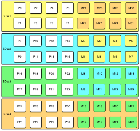
Unless both the primary and mirror of the same segment instance fail, up to half of your hosts can fail and the cluster will continue to run as long as resources (CPU, memory, and IO) are sufficient to meet the needs.
Any host failure will degrade performance by half or more because the host with the mirrors will have twice the number of active primaries. If your resource utilization is normally greater than 50%, you will have to adjust your workload until the failed host is recovered or replaced. If you normally run at less than 50% resource utilization the cluster can continue to operate at a degraded level of performance until the failure is corrected.
Spread Mirroring
With spread mirroring, mirrors for each host’s primary segments are spread across as many hosts as there are segments per host. Spread mirroring is easy to set up when the cluster is initialized, but requires that the cluster have at least one more host than there are segments per host.
The following diagram shows the spread mirroring configuration for a cluster with three primaries on four hosts.
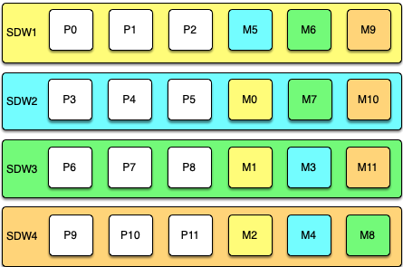
Expanding a cluster with spread mirroring requires more planning and may take more time. You must either add a set of hosts equal to the number of primaries per host plus one, or you can add two nodes in a group mirroring configuration and, when the expansion is complete, move mirrors to recreate the spread mirror configuration.
Spread mirroring has the least performance impact for a single failed host because each host’s mirrors are spread across the maximum number of hosts. Load is increased by 1/Nth, where N is the number of primaries per host. Spread mirroring is, however, the most likely configuration to have a catastrophic failure if two or more hosts fail simultaneously.
Block Mirroring
With block mirroring, nodes are divided into blocks, for example a block of four or eight hosts, and the mirrors for segments on each host are placed on other hosts within the block. Depending on the number of hosts in the block and the number of primary segments per host, each host maintains more than one mirror for each other host’s segments.
The following diagram shows a single block mirroring configuration for a block of four hosts, each with eight primary segments:
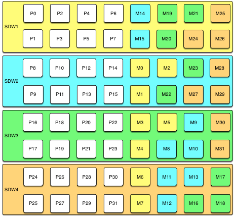
If there are eight hosts, an additional four-host block is added with the mirrors for primary segments 32 through 63 set up in the same pattern.
A cluster with block mirroring is easy to expand because each block is a self-contained primary mirror group. The cluster is expanded by adding one or more blocks. There is no need to move mirrors after expansion to maintain a consistent mirror setup. This configuration is able to survive multiple host failures as long as the failed hosts are in different blocks.
Because each host in a block has multiple mirror instances for each other host in the block, block mirroring has a higher performance impact for host failures than spread mirroring, but a lower impact than group mirroring. The expected performance impact varies by block size and primary segments per node. As with group mirroring, if the resources are available, performance will be negatively impacted but the cluster will remain available. If resources are insufficient to accommodate the added load you must reduce the workload until the failed node is replaced.
Implementing Block Mirroring
Block mirroring is not one of the automatic options SynxDB offers when you set up or expand a cluster. To use it, you must create your own configuration.
For a new SynxDB system, you can initialize the cluster without mirrors, and then run gpaddmirrors -i mirror_config_file with a custom mirror configuration file to create the mirrors for each block. You must create the file system locations for the mirror segments before you run gpaddmirrors. See the gpaddmirrors reference page in the SynxDB Management Utility Guide for details.
If you expand a system that has block mirroring or you want to implement block mirroring at the same time you expand a cluster, it is recommended that you complete the expansion first, using the default grouping mirror configuration, and then use the gpmovemirrors utility to move mirrors into the block configuration.
To implement block mirroring with an existing system that has a different mirroring scheme, you must first determine the desired location for each mirror according to your block configuration, and then determine which of the existing mirrors must be relocated. Follow these steps:
-
Run the following query to find the current locations of the primary and mirror segments:
SELECT dbid, content, role, port, hostname, datadir FROM gp_segment_configuration WHERE content > -1 ;The
gp_segment_configurationsystem catalog table contains the current segment configuration. -
Create a list with the current mirror location and the desired block mirroring location, then remove any mirrors from the list that are already on the correct host.
-
Create an input file for the
gpmovemirrorsutility with an entry for each mirror that must be moved.The
gpmovemirrorsinput file has the following format:old_address|port|data_dir new_address|port|data_dirWhere
old_addressis the host name or IP address of the segment host, port is the communication port, anddata_diris the segment instance data directory.The following example
gpmovemirrorsinput file specifies three mirror segments to move.sdw2|50001|/data2/mirror/gpseg1 sdw3|50001|/data/mirror/gpseg1 sdw2|50001|/data2/mirror/gpseg2 sdw4|50001|/data/mirror/gpseg2 sdw3|50001|/data2/mirror/gpseg3 sdw1|50001|/data/mirror/gpseg3 -
Run
gpmovemirrorswith a command like the following:gpmovemirrors -i mirror_config_file
The gpmovemirrors utility validates the input file, calls gprecoverseg to relocate each specified mirror, and removes the original mirror. It creates a backout configuration file which can be used as input to gpmovemirrors to undo the changes that were made. The backout file has the same name as the input file, with the suffix _backout_timestamp added.
See the SynxDB Management Utility Reference for complete information about the gpmovemirrors utility.
SynxDB Reference Guide
Reference information for SynxDB systems including SQL commands, system catalogs, environment variables, server configuration parameters, character set support, datatypes, and SynxDB extensions.
SQL Commands
The following SQL commands are available in SynxDB:
- ABORT
- ALTER AGGREGATE
- ALTER COLLATION
- ALTER CONVERSION
- ALTER DATABASE
- ALTER DEFAULT PRIVILEGES
- ALTER DOMAIN
- ALTER EXTERNAL TABLE
- ALTER FOREIGN DATA WRAPPER
- ALTER FOREIGN TABLE
- ALTER FUNCTION
- ALTER GROUP
- ALTER INDEX
- ALTER LANGUAGE
- ALTER OPERATOR
- ALTER OPERATOR CLASS
- ALTER OPERATOR FAMILY
- ALTER PROTOCOL
- ALTER RESOURCE GROUP
- ALTER RESOURCE QUEUE
- ALTER ROLE
- ALTER RULE
- ALTER SCHEMA
- ALTER SEQUENCE
- ALTER SERVER
- ALTER TABLE
- ALTER TABLESPACE
- ALTER TEXT SEARCH CONFIGURATION
- ALTER TEXT SEARCH DICTIONARY
- ALTER TEXT SEARCH PARSER
- ALTER TEXT SEARCH TEMPLATE
- ALTER TYPE
- ALTER USER
- ALTER USER MAPPING
- ALTER VIEW
- ANALYZE
- BEGIN
- CHECKPOINT
- CLOSE
- CLUSTER
- COMMENT
- COMMIT
- COPY
- CREATE AGGREGATE
- CREATE CAST
- CREATE COLLATION
- CREATE CONVERSION
- CREATE DATABASE
- CREATE DOMAIN
- CREATE EXTERNAL TABLE
- CREATE FOREIGN DATA WRAPPER
- CREATE FOREIGN TABLE
- CREATE FUNCTION
- CREATE GROUP
- CREATE INDEX
- CREATE LANGUAGE
- CREATE OPERATOR
- CREATE OPERATOR CLASS
- CREATE OPERATOR FAMILY
- CREATE PROTOCOL
- CREATE RESOURCE GROUP
- CREATE RESOURCE QUEUE
- CREATE ROLE
- CREATE RULE
- CREATE SCHEMA
- CREATE SEQUENCE
- CREATE SERVER
- CREATE TABLE
- CREATE TABLE AS
- CREATE TABLESPACE
- CREATE TEXT SEARCH CONFIGURATION
- CREATE TEXT SEARCH DICTIONARY
- CREATE TEXT SEARCH PARSER
- CREATE TEXT SEARCH TEMPLATE
- CREATE TYPE
- CREATE USER
- CREATE USER MAPPING
- CREATE VIEW
- DEALLOCATE
- DECLARE
- DELETE
- DISCARD
- DO
- DROP AGGREGATE
- DROP CAST
- DROP COLLATION
- DROP CONVERSION
- DROP DATABASE
- DROP DOMAIN
- DROP EXTERNAL TABLE
- DROP FOREIGN DATA WRAPPER
- DROP FOREIGN TABLE
- DROP FUNCTION
- DROP GROUP
- DROP INDEX
- DROP LANGUAGE
- DROP OPERATOR
- DROP OPERATOR CLASS
- DROP OPERATOR FAMILY
- DROP OWNED
- DROP PROTOCOL
- DROP RESOURCE GROUP
- DROP RESOURCE QUEUE
- DROP ROLE
- DROP RULE
- DROP SCHEMA
- DROP SEQUENCE
- DROP SERVER
- DROP TABLE
- DROP TABLESPACE
- DROP TEXT SEARCH CONFIGURATION
- DROP TEXT SEARCH DICTIONARY
- DROP TEXT SEARCH PARSER
- DROP TEXT SEARCH TEMPLATE
- DROP TYPE
- DROP USER
- DROP USER MAPPING
- DROP VIEW
- END
- EXECUTE
- EXPLAIN
- FETCH
- GRANT
- INSERT
- LISTEN
- LOAD
- LOCK
- MOVE
- NOTIFY
- PREPARE
- REASSIGN OWNED
- REINDEX
- RELEASE SAVEPOINT
- RESET
- RETRIEVE
- REVOKE
- ROLLBACK
- ROLLBACK TO SAVEPOINT
- SAVEPOINT
- SELECT
- SELECT INTO
- SET
- SET CONSTRAINTS
- SET ROLE
- SET SESSION AUTHORIZATION
- SET TRANSACTION
- SHOW
- START TRANSACTION
- TRUNCATE
- UNLISTEN
- UPDATE
- VACUUM
- VALUES
* Not implemented in 5.0
SQL Syntax Summary
ABORT
Terminates the current transaction.
ABORT [WORK | TRANSACTION]
See ABORT for more information.
ALTER AGGREGATE
Changes the definition of an aggregate function
ALTER AGGREGATE <name> ( <aggregate_signature> ) RENAME TO <new_name>
ALTER AGGREGATE <name> ( <aggregate_signature> ) OWNER TO <new_owner>
ALTER AGGREGATE <name> ( <aggregate_signature> ) SET SCHEMA <new_schema>
See ALTER AGGREGATE for more information.
ALTER COLLATION
Changes the definition of a collation.
ALTER COLLATION <name> RENAME TO <new_name>
ALTER COLLATION <name> OWNER TO <new_owner>
ALTER COLLATION <name> SET SCHEMA <new_schema>
See ALTER COLLATION for more information.
ALTER CONVERSION
Changes the definition of a conversion.
ALTER CONVERSION <name> RENAME TO <newname>
ALTER CONVERSION <name> OWNER TO <newowner>
ALTER CONVERSION <name> SET SCHEMA <new_schema>
See ALTER CONVERSION for more information.
ALTER DATABASE
Changes the attributes of a database.
ALTER DATABASE <name> [ WITH CONNECTION LIMIT <connlimit> ]
ALTER DATABASE <name> RENAME TO <newname>
ALTER DATABASE <name> OWNER TO <new_owner>
ALTER DATABASE <name> SET TABLESPACE <new_tablespace>
ALTER DATABASE <name> SET <parameter> { TO | = } { <value> | DEFAULT }
ALTER DATABASE <name> SET <parameter> FROM CURRENT
ALTER DATABASE <name> RESET <parameter>
ALTER DATABASE <name> RESET ALL
See ALTER DATABASE for more information.
ALTER DEFAULT PRIVILEGES
Changes default access privileges.
ALTER DEFAULT PRIVILEGES
[ FOR { ROLE | USER } <target_role> [, ...] ]
[ IN SCHEMA <schema_name> [, ...] ]
<abbreviated_grant_or_revoke>
where <abbreviated_grant_or_revoke> is one of:
GRANT { { SELECT | INSERT | UPDATE | DELETE | TRUNCATE | REFERENCES | TRIGGER }
[, ...] | ALL [ PRIVILEGES ] }
ON TABLES
TO { [ GROUP ] <role_name> | PUBLIC } [, ...] [ WITH GRANT OPTION ]
GRANT { { USAGE | SELECT | UPDATE }
[, ...] | ALL [ PRIVILEGES ] }
ON SEQUENCES
TO { [ GROUP ] <role_name> | PUBLIC } [, ...] [ WITH GRANT OPTION ]
GRANT { EXECUTE | ALL [ PRIVILEGES ] }
ON FUNCTIONS
TO { [ GROUP ] <role_name> | PUBLIC } [, ...] [ WITH GRANT OPTION ]
GRANT { USAGE | ALL [ PRIVILEGES ] }
ON TYPES
TO { [ GROUP ] <role_name> | PUBLIC } [, ...] [ WITH GRANT OPTION ]
REVOKE [ GRANT OPTION FOR ]
{ { SELECT | INSERT | UPDATE | DELETE | TRUNCATE | REFERENCES | TRIGGER }
[, ...] | ALL [ PRIVILEGES ] }
ON TABLES
FROM { [ GROUP ] <role_name> | PUBLIC } [, ...]
[ CASCADE | RESTRICT ]
REVOKE [ GRANT OPTION FOR ]
{ { USAGE | SELECT | UPDATE }
[, ...] | ALL [ PRIVILEGES ] }
ON SEQUENCES
FROM { [ GROUP ] <role_name> | PUBLIC } [, ...]
[ CASCADE | RESTRICT ]
REVOKE [ GRANT OPTION FOR ]
{ EXECUTE | ALL [ PRIVILEGES ] }
ON FUNCTIONS
FROM { [ GROUP ] <role_name> | PUBLIC } [, ...]
[ CASCADE | RESTRICT ]
REVOKE [ GRANT OPTION FOR ]
{ USAGE | ALL [ PRIVILEGES ] }
ON TYPES
FROM { [ GROUP ] <role_name> | PUBLIC } [, ...]
[ CASCADE | RESTRICT ]
See ALTER DEFAULT PRIVILEGES for more information.
ALTER DOMAIN
Changes the definition of a domain.
ALTER DOMAIN <name> { SET DEFAULT <expression> | DROP DEFAULT }
ALTER DOMAIN <name> { SET | DROP } NOT NULL
ALTER DOMAIN <name> ADD <domain_constraint> [ NOT VALID ]
ALTER DOMAIN <name> DROP CONSTRAINT [ IF EXISTS ] <constraint_name> [RESTRICT | CASCADE]
ALTER DOMAIN <name> RENAME CONSTRAINT <constraint_name> TO <new_constraint_name>
ALTER DOMAIN <name> VALIDATE CONSTRAINT <constraint_name>
ALTER DOMAIN <name> OWNER TO <new_owner>
ALTER DOMAIN <name> RENAME TO <new_name>
ALTER DOMAIN <name> SET SCHEMA <new_schema>
See ALTER DOMAIN for more information.
ALTER EXTENSION
Change the definition of an extension that is registered in a SynxDB database.
ALTER EXTENSION <name> UPDATE [ TO <new_version> ]
ALTER EXTENSION <name> SET SCHEMA <new_schema>
ALTER EXTENSION <name> ADD <member_object>
ALTER EXTENSION <name> DROP <member_object>
where <member_object> is:
ACCESS METHOD <object_name> |
AGGREGATE <aggregate_name> ( <aggregate_signature> ) |
CAST (<source_type> AS <target_type>) |
COLLATION <object_name> |
CONVERSION <object_name> |
DOMAIN <object_name> |
EVENT TRIGGER <object_name> |
FOREIGN DATA WRAPPER <object_name> |
FOREIGN TABLE <object_name> |
FUNCTION <function_name> ( [ [ <argmode> ] [ <argname> ] <argtype> [, ...] ] ) |
MATERIALIZED VIEW <object_name> |
OPERATOR <operator_name> (<left_type>, <right_type>) |
OPERATOR CLASS <object_name> USING <index_method> |
OPERATOR FAMILY <object_name> USING <index_method> |
[ PROCEDURAL ] LANGUAGE <object_name> |
SCHEMA <object_name> |
SEQUENCE <object_name> |
SERVER <object_name> |
TABLE <object_name> |
TEXT SEARCH CONFIGURATION <object_name> |
TEXT SEARCH DICTIONARY <object_name> |
TEXT SEARCH PARSER <object_name> |
TEXT SEARCH TEMPLATE <object_name> |
TRANSFORM FOR <type_name> LANGUAGE <lang_name> |
TYPE <object_name> |
VIEW <object_name>
and <aggregate_signature> is:
* |
[ <argmode> ] [ <argname> ] <argtype> [ , ... ] |
[ [ <argmode> ] [ <argname> ] <argtype> [ , ... ] ] ORDER BY [ <argmode> ] [ <argname> ] <argtype> [ , ... ]
See ALTER EXTENSION for more information.
ALTER EXTERNAL TABLE
Changes the definition of an external table.
ALTER EXTERNAL TABLE <name> <action> [, ... ]
where action is one of:
ADD [COLUMN] <new_column> <type>
DROP [COLUMN] <column> [RESTRICT|CASCADE]
ALTER [COLUMN] <column> TYPE <type>
OWNER TO <new_owner>
See ALTER EXTERNAL TABLE for more information.
ALTER FOREIGN DATA WRAPPER
Changes the definition of a foreign-data wrapper.
ALTER FOREIGN DATA WRAPPER <name>
[ HANDLER <handler_function> | NO HANDLER ]
[ VALIDATOR <validator_function> | NO VALIDATOR ]
[ OPTIONS ( [ ADD | SET | DROP ] <option> ['<value>'] [, ... ] ) ]
ALTER FOREIGN DATA WRAPPER <name> OWNER TO <new_owner>
ALTER FOREIGN DATA WRAPPER <name> RENAME TO <new_name>
See ALTER FOREIGN DATA WRAPPER for more information.
ALTER FOREIGN TABLE
Changes the definition of a foreign table.
ALTER FOREIGN TABLE [ IF EXISTS ] <name>
<action> [, ... ]
ALTER FOREIGN TABLE [ IF EXISTS ] <name>
RENAME [ COLUMN ] <column_name> TO <new_column_name>
ALTER FOREIGN TABLE [ IF EXISTS ] <name>
RENAME TO <new_name>
ALTER FOREIGN TABLE [ IF EXISTS ] <name>
SET SCHEMA <new_schema>
See ALTER FOREIGN TABLE for more information.
ALTER FUNCTION
Changes the definition of a function.
ALTER FUNCTION <name> ( [ [<argmode>] [<argname>] <argtype> [, ...] ] )
<action> [, ... ] [RESTRICT]
ALTER FUNCTION <name> ( [ [<argmode>] [<argname>] <argtype> [, ...] ] )
RENAME TO <new_name>
ALTER FUNCTION <name> ( [ [<argmode>] [<argname>] <argtype> [, ...] ] )
OWNER TO <new_owner>
ALTER FUNCTION <name> ( [ [<argmode>] [<argname>] <argtype> [, ...] ] )
SET SCHEMA <new_schema>
See ALTER FUNCTION for more information.
ALTER GROUP
Changes a role name or membership.
ALTER GROUP <groupname> ADD USER <username> [, ... ]
ALTER GROUP <groupname> DROP USER <username> [, ... ]
ALTER GROUP <groupname> RENAME TO <newname>
See ALTER GROUP for more information.
ALTER INDEX
Changes the definition of an index.
ALTER INDEX [ IF EXISTS ] <name> RENAME TO <new_name>
ALTER INDEX [ IF EXISTS ] <name> SET TABLESPACE <tablespace_name>
ALTER INDEX [ IF EXISTS ] <name> SET ( <storage_parameter> = <value> [, ...] )
ALTER INDEX [ IF EXISTS ] <name> RESET ( <storage_parameter> [, ...] )
ALTER INDEX ALL IN TABLESPACE <name> [ OWNED BY <role_name> [, ... ] ]
SET TABLESPACE <new_tablespace> [ NOWAIT ]
See ALTER INDEX for more information.
ALTER LANGUAGE
Changes the name of a procedural language.
ALTER LANGUAGE <name> RENAME TO <newname>
ALTER LANGUAGE <name> OWNER TO <new_owner>
See ALTER LANGUAGE for more information.
ALTER MATERIALIZED VIEW
Changes the definition of a materialized view.
ALTER MATERIALIZED VIEW [ IF EXISTS ] <name> <action> [, ... ]
ALTER MATERIALIZED VIEW [ IF EXISTS ] <name>
RENAME [ COLUMN ] <column_name> TO <new_column_name>
ALTER MATERIALIZED VIEW [ IF EXISTS ] <name>
RENAME TO <new_name>
ALTER MATERIALIZED VIEW [ IF EXISTS ] <name>
SET SCHEMA <new_schema>
ALTER MATERIALIZED VIEW ALL IN TABLESPACE <name> [ OWNED BY <role_name> [, ... ] ]
SET TABLESPACE <new_tablespace> [ NOWAIT ]
where <action> is one of:
ALTER [ COLUMN ] <column_name> SET STATISTICS <integer>
ALTER [ COLUMN ] <column_name> SET ( <attribute_option> = <value> [, ... ] )
ALTER [ COLUMN ] <column_name> RESET ( <attribute_option> [, ... ] )
ALTER [ COLUMN ] <column_name> SET STORAGE { PLAIN | EXTERNAL | EXTENDED | MAIN }
CLUSTER ON <index_name>
SET WITHOUT CLUSTER
SET ( <storage_paramete>r = <value> [, ... ] )
RESET ( <storage_parameter> [, ... ] )
OWNER TO <new_owner>
See ALTER MATERIALIZED VIEW for more information.
ALTER OPERATOR
Changes the definition of an operator.
ALTER OPERATOR <name> ( {<left_type> | NONE} , {<right_type> | NONE} )
OWNER TO <new_owner>
ALTER OPERATOR <name> ( {<left_type> | NONE} , {<right_type> | NONE} )
SET SCHEMA <new_schema>
See ALTER OPERATOR for more information.
ALTER OPERATOR CLASS
Changes the definition of an operator class.
ALTER OPERATOR CLASS <name> USING <index_method> RENAME TO <new_name>
ALTER OPERATOR CLASS <name> USING <index_method> OWNER TO <new_owner>
ALTER OPERATOR CLASS <name> USING <index_method> SET SCHEMA <new_schema>
See ALTER OPERATOR CLASS for more information.
ALTER OPERATOR FAMILY
Changes the definition of an operator family.
ALTER OPERATOR FAMILY <name> USING <index_method> ADD
{ OPERATOR <strategy_number> <operator_name> ( <op_type>, <op_type> ) [ FOR SEARCH | FOR ORDER BY <sort_family_name> ]
| FUNCTION <support_number> [ ( <op_type> [ , <op_type> ] ) ] <funcname> ( <argument_type> [, ...] )
} [, ... ]
ALTER OPERATOR FAMILY <name> USING <index_method> DROP
{ OPERATOR <strategy_number> ( <op_type>, <op_type> )
| FUNCTION <support_number> [ ( <op_type> [ , <op_type> ] )
} [, ... ]
ALTER OPERATOR FAMILY <name> USING <index_method> RENAME TO <new_name>
ALTER OPERATOR FAMILY <name> USING <index_method> OWNER TO <new_owner>
ALTER OPERATOR FAMILY <name> USING <index_method> SET SCHEMA <new_schema>
See ALTER OPERATOR FAMILY for more information.
ALTER PROTOCOL
Changes the definition of a protocol.
ALTER PROTOCOL <name> RENAME TO <newname>
ALTER PROTOCOL <name> OWNER TO <newowner>
See ALTER PROTOCOL for more information.
ALTER RESOURCE GROUP
Changes the limits of a resource group.
ALTER RESOURCE GROUP <name> SET <group_attribute> <value>
See ALTER RESOURCE GROUP for more information.
ALTER RESOURCE QUEUE
Changes the limits of a resource queue.
ALTER RESOURCE QUEUE <name> WITH ( <queue_attribute>=<value> [, ... ] )
See ALTER RESOURCE QUEUE for more information.
ALTER ROLE
Changes a database role (user or group).
ALTER ROLE <name> [ [ WITH ] <option> [ ... ] ]
where <option> can be:
SUPERUSER | NOSUPERUSER
| CREATEDB | NOCREATEDB
| CREATEROLE | NOCREATEROLE
| CREATEEXTTABLE | NOCREATEEXTTABLE [ ( attribute='value' [, ...] )
where attributes and values are:
type='readable'|'writable'
protocol='gpfdist'|'http'
| INHERIT | NOINHERIT
| LOGIN | NOLOGIN
| REPLICATION | NOREPLICATION
| CONNECTION LIMIT <connlimit>
| [ ENCRYPTED | UNENCRYPTED ] PASSWORD '<password>'
| VALID UNTIL '<timestamp>'
ALTER ROLE <name> RENAME TO <new_name>
ALTER ROLE { <name> | ALL } [ IN DATABASE <database_name> ] SET <configuration_parameter> { TO | = } { <value> | DEFAULT }
ALTER ROLE { <name> | ALL } [ IN DATABASE <database_name> ] SET <configuration_parameter> FROM CURRENT
ALTER ROLE { <name> | ALL } [ IN DATABASE <database_name> ] RESET <configuration_parameter>
ALTER ROLE { <name> | ALL } [ IN DATABASE <database_name> ] RESET ALL
ALTER ROLE <name> RESOURCE QUEUE {<queue_name> | NONE}
ALTER ROLE <name> RESOURCE GROUP {<group_name> | NONE}
See ALTER ROLE for more information.
ALTER RULE
Changes the definition of a rule.
ALTER RULE name ON table\_name RENAME TO new\_name
See ALTER RULE for more information.
ALTER SCHEMA
Changes the definition of a schema.
ALTER SCHEMA <name> RENAME TO <newname>
ALTER SCHEMA <name> OWNER TO <newowner>
See ALTER SCHEMA for more information.
ALTER SEQUENCE
Changes the definition of a sequence generator.
ALTER SEQUENCE [ IF EXISTS ] <name> [INCREMENT [ BY ] <increment>]
[MINVALUE <minvalue> | NO MINVALUE]
[MAXVALUE <maxvalue> | NO MAXVALUE]
[START [ WITH ] <start> ]
[RESTART [ [ WITH ] <restart>] ]
[CACHE <cache>] [[ NO ] CYCLE]
[OWNED BY {<table.column> | NONE}]
ALTER SEQUENCE [ IF EXISTS ] <name> OWNER TO <new_owner>
ALTER SEQUENCE [ IF EXISTS ] <name> RENAME TO <new_name>
ALTER SEQUENCE [ IF EXISTS ] <name> SET SCHEMA <new_schema>
See ALTER SEQUENCE for more information.
ALTER SERVER
Changes the definition of a foreign server.
ALTER SERVER <server_name> [ VERSION '<new_version>' ]
[ OPTIONS ( [ ADD | SET | DROP ] <option> ['<value>'] [, ... ] ) ]
ALTER SERVER <server_name> OWNER TO <new_owner>
ALTER SERVER <server_name> RENAME TO <new_name>
See ALTER SERVER for more information.
ALTER TABLE
Changes the definition of a table.
ALTER TABLE [IF EXISTS] [ONLY] <name>
<action> [, ... ]
ALTER TABLE [IF EXISTS] [ONLY] <name>
RENAME [COLUMN] <column_name> TO <new_column_name>
ALTER TABLE [ IF EXISTS ] [ ONLY ] <name>
RENAME CONSTRAINT <constraint_name> TO <new_constraint_name>
ALTER TABLE [IF EXISTS] <name>
RENAME TO <new_name>
ALTER TABLE [IF EXISTS] <name>
SET SCHEMA <new_schema>
ALTER TABLE ALL IN TABLESPACE <name> [ OWNED BY <role_name> [, ... ] ]
SET TABLESPACE <new_tablespace> [ NOWAIT ]
ALTER TABLE [IF EXISTS] [ONLY] <name> SET
WITH (REORGANIZE=true|false)
| DISTRIBUTED BY ({<column_name> [<opclass>]} [, ... ] )
| DISTRIBUTED RANDOMLY
| DISTRIBUTED REPLICATED
ALTER TABLE <name>
[ ALTER PARTITION { <partition_name> | FOR (RANK(<number>))
| FOR (<value>) } [...] ] <partition_action>
where <action> is one of:
ADD [COLUMN] <column_name data_type> [ DEFAULT <default_expr> ]
[<column_constraint> [ ... ]]
[ COLLATE <collation> ]
[ ENCODING ( <storage_parameter> [,...] ) ]
DROP [COLUMN] [IF EXISTS] <column_name> [RESTRICT | CASCADE]
ALTER [COLUMN] <column_name> [ SET DATA ] TYPE <type> [COLLATE <collation>] [USING <expression>]
ALTER [COLUMN] <column_name> SET DEFAULT <expression>
ALTER [COLUMN] <column_name> DROP DEFAULT
ALTER [COLUMN] <column_name> { SET | DROP } NOT NULL
ALTER [COLUMN] <column_name> SET STATISTICS <integer>
ALTER [COLUMN] column SET ( <attribute_option> = <value> [, ... ] )
ALTER [COLUMN] column RESET ( <attribute_option> [, ... ] )
ADD <table_constraint> [NOT VALID]
ADD <table_constraint_using_index>
VALIDATE CONSTRAINT <constraint_name>
DROP CONSTRAINT [IF EXISTS] <constraint_name> [RESTRICT | CASCADE]
DISABLE TRIGGER [<trigger_name> | ALL | USER]
ENABLE TRIGGER [<trigger_name> | ALL | USER]
CLUSTER ON <index_name>
SET WITHOUT CLUSTER
SET WITHOUT OIDS
SET (<storage_parameter> = <value>)
RESET (<storage_parameter> [, ... ])
INHERIT <parent_table>
NO INHERIT <parent_table>
OF `type_name`
NOT OF
OWNER TO <new_owner>
SET TABLESPACE <new_tablespace>
See ALTER TABLE for more information.
ALTER TABLESPACE
Changes the definition of a tablespace.
ALTER TABLESPACE <name> RENAME TO <new_name>
ALTER TABLESPACE <name> OWNER TO <new_owner>
ALTER TABLESPACE <name> SET ( <tablespace_option> = <value> [, ... ] )
ALTER TABLESPACE <name> RESET ( <tablespace_option> [, ... ] )
See ALTER TABLESPACE for more information.
ALTER TEXT SEARCH CONFIGURATION
Changes the definition of a text search configuration.
ALTER TEXT SEARCH CONFIGURATION <name>
ALTER MAPPING FOR <token_type> [, ... ] WITH <dictionary_name> [, ... ]
ALTER TEXT SEARCH CONFIGURATION <name>
ALTER MAPPING REPLACE <old_dictionary> WITH <new_dictionary>
ALTER TEXT SEARCH CONFIGURATION <name>
ALTER MAPPING FOR <token_type> [, ... ] REPLACE <old_dictionary> WITH <new_dictionary>
ALTER TEXT SEARCH CONFIGURATION <name>
DROP MAPPING [ IF EXISTS ] FOR <token_type> [, ... ]
ALTER TEXT SEARCH CONFIGURATION <name> RENAME TO <new_name>
ALTER TEXT SEARCH CONFIGURATION <name> OWNER TO <new_owner>
ALTER TEXT SEARCH CONFIGURATION <name> SET SCHEMA <new_schema>
See ALTER TEXT SEARCH CONFIGURATION for more information.
ALTER TEXT SEARCH DICTIONARY
Changes the definition of a text search dictionary.
ALTER TEXT SEARCH DICTIONARY <name> (
<option> [ = <value> ] [, ... ]
)
ALTER TEXT SEARCH DICTIONARY <name> RENAME TO <new_name>
ALTER TEXT SEARCH DICTIONARY <name> OWNER TO <new_owner>
ALTER TEXT SEARCH DICTIONARY <name> SET SCHEMA <new_schema>
See ALTER TEXT SEARCH DICTIONARY for more information.
ALTER TEXT SEARCH PARSER
Changes the definition of a text search parser.
ALTER TEXT SEARCH PARSER <name> RENAME TO <new_name>
ALTER TEXT SEARCH PARSER <name> SET SCHEMA <new_schema>
See ALTER TEXT SEARCH PARSER for more information.
ALTER TEXT SEARCH TEMPLATE
Changes the definition of a text search template.
ALTER TEXT SEARCH TEMPLATE <name> RENAME TO <new_name>
ALTER TEXT SEARCH TEMPLATE <name> SET SCHEMA <new_schema>
See ALTER TEXT SEARCH TEMPLATE for more information.
ALTER TYPE
Changes the definition of a data type.
ALTER TYPE <name> <action> [, ... ]
ALTER TYPE <name> OWNER TO <new_owner>
ALTER TYPE <name> RENAME ATTRIBUTE <attribute_name> TO <new_attribute_name> [ CASCADE | RESTRICT ]
ALTER TYPE <name> RENAME TO <new_name>
ALTER TYPE <name> SET SCHEMA <new_schema>
ALTER TYPE <name> ADD VALUE [ IF NOT EXISTS ] <new_enum_value> [ { BEFORE | AFTER } <existing_enum_value> ]
ALTER TYPE <name> SET DEFAULT ENCODING ( <storage_directive> )
where <action> is one of:
ADD ATTRIBUTE <attribute_name> <data_type> [ COLLATE <collation> ] [ CASCADE | RESTRICT ]
DROP ATTRIBUTE [ IF EXISTS ] <attribute_name> [ CASCADE | RESTRICT ]
ALTER ATTRIBUTE <attribute_name> [ SET DATA ] TYPE <data_type> [ COLLATE <collation> ] [ CASCADE | RESTRICT ]
See ALTER TYPE for more information.
ALTER USER
Changes the definition of a database role (user).
ALTER USER <name> RENAME TO <newname>
ALTER USER <name> SET <config_parameter> {TO | =} {<value> | DEFAULT}
ALTER USER <name> RESET <config_parameter>
ALTER USER <name> RESOURCE QUEUE {<queue_name> | NONE}
ALTER USER <name> RESOURCE GROUP {<group_name> | NONE}
ALTER USER <name> [ [WITH] <option> [ ... ] ]
See ALTER USER for more information.
ALTER USER MAPPING
Changes the definition of a user mapping for a foreign server.
ALTER USER MAPPING FOR { <username> | USER | CURRENT_USER | PUBLIC }
SERVER <servername>
OPTIONS ( [ ADD | SET | DROP ] <option> ['<value>'] [, ... ] )
See ALTER USER MAPPING for more information.
ALTER VIEW
Changes properties of a view.
ALTER VIEW [ IF EXISTS ] <name> ALTER [ COLUMN ] <column_name> SET DEFAULT <expression>
ALTER VIEW [ IF EXISTS ] <name> ALTER [ COLUMN ] <column_name> DROP DEFAULT
ALTER VIEW [ IF EXISTS ] <name> OWNER TO <new_owner>
ALTER VIEW [ IF EXISTS ] <name> RENAME TO <new_name>
ALTER VIEW [ IF EXISTS ] <name> SET SCHEMA <new_schema>
ALTER VIEW [ IF EXISTS ] <name> SET ( <view_option_name> [= <view_option_value>] [, ... ] )
ALTER VIEW [ IF EXISTS ] <name> RESET ( <view_option_name> [, ... ] )
See ALTER VIEW for more information.
ANALYZE
Collects statistics about a database.
ANALYZE [VERBOSE] [<table> [ (<column> [, ...] ) ]]
ANALYZE [VERBOSE] {<root_partition_table_name>|<leaf_partition_table_name>} [ (<column> [, ...] )]
ANALYZE [VERBOSE] ROOTPARTITION {ALL | <root_partition_table_name> [ (<column> [, ...] )]}
See ANALYZE for more information.
BEGIN
Starts a transaction block.
BEGIN [WORK | TRANSACTION] [<transaction_mode>]
See BEGIN for more information.
CHECKPOINT
Forces a transaction log checkpoint.
CHECKPOINT
See CHECKPOINT for more information.
CLOSE
Closes a cursor.
CLOSE <cursor_name>
See CLOSE for more information.
CLUSTER
Physically reorders a heap storage table on disk according to an index. Not a recommended operation in SynxDB.
CLUSTER <indexname> ON <tablename>
CLUSTER [VERBOSE] <tablename> [ USING index_name ]
CLUSTER [VERBOSE]
See CLUSTER for more information.
COMMENT
Defines or changes the comment of an object.
COMMENT ON
{ TABLE <object_name> |
COLUMN <relation_name.column_name> |
AGGREGATE <agg_name> (<agg_signature>) |
CAST (<source_type> AS <target_type>) |
COLLATION <object_name>
CONSTRAINT <constraint_name> ON <table_name> |
CONVERSION <object_name> |
DATABASE <object_name> |
DOMAIN <object_name> |
EXTENSION <object_name> |
FOREIGN DATA WRAPPER <object_name> |
FOREIGN TABLE <object_name> |
FUNCTION <func_name> ([[<argmode>] [<argname>] <argtype> [, ...]]) |
INDEX <object_name> |
LARGE OBJECT <large_object_oid> |
MATERIALIZED VIEW <object_name> |
OPERATOR <operator_name> (<left_type>, <right_type>) |
OPERATOR CLASS <object_name> USING <index_method> |
[PROCEDURAL] LANGUAGE <object_name> |
RESOURCE GROUP <object_name> |
RESOURCE QUEUE <object_name> |
ROLE <object_name> |
RULE <rule_name> ON <table_name> |
SCHEMA <object_name> |
SEQUENCE <object_name> |
SERVER <object_name> |
TABLESPACE <object_name> |
TEXT SEARCH CONFIGURATION <object_name> |
TEXT SEARCH DICTIONARY <object_name> |
TEXT SEARCH PARSER <object_name> |
TEXT SEARCH TEMPLATE <object_name> |
TRIGGER <trigger_name> ON <table_name> |
TYPE <object_name> |
VIEW <object_name> }
IS '<text>'
See COMMENT for more information.
COMMIT
Commits the current transaction.
COMMIT [WORK | TRANSACTION]
See COMMIT for more information.
COPY
Copies data between a file and a table.
COPY <table_name> [(<column_name> [, ...])]
FROM {'<filename>' | PROGRAM '<command>' | STDIN}
[ [ WITH ] ( <option> [, ...] ) ]
[ ON SEGMENT ]
COPY { <table_name> [(<column_name> [, ...])] | (<query>)}
TO {'<filename>' | PROGRAM '<command>' | STDOUT}
[ [ WITH ] ( <option> [, ...] ) ]
[ ON SEGMENT ]
See COPY for more information.
CREATE AGGREGATE
Defines a new aggregate function.
CREATE AGGREGATE <name> ( [ <argmode> ] [ <argname> ] <arg_data_type> [ , ... ] ) (
SFUNC = <statefunc>,
STYPE = <state_data_type>
[ , SSPACE = <state_data_size> ]
[ , FINALFUNC = <ffunc> ]
[ , FINALFUNC_EXTRA ]
[ , COMBINEFUNC = <combinefunc> ]
[ , SERIALFUNC = <serialfunc> ]
[ , DESERIALFUNC = <deserialfunc> ]
[ , INITCOND = <initial_condition> ]
[ , MSFUNC = <msfunc> ]
[ , MINVFUNC = <minvfunc> ]
[ , MSTYPE = <mstate_data_type> ]
[ , MSSPACE = <mstate_data_size> ]
[ , MFINALFUNC = <mffunc> ]
[ , MFINALFUNC_EXTRA ]
[ , MINITCOND = <minitial_condition> ]
[ , SORTOP = <sort_operator> ]
)
CREATE AGGREGATE <name> ( [ [ <argmode> ] [ <argname> ] <arg_data_type> [ , ... ] ]
ORDER BY [ <argmode> ] [ <argname> ] <arg_data_type> [ , ... ] ) (
SFUNC = <statefunc>,
STYPE = <state_data_type>
[ , SSPACE = <state_data_size> ]
[ , FINALFUNC = <ffunc> ]
[ , FINALFUNC_EXTRA ]
[ , COMBINEFUNC = <combinefunc> ]
[ , SERIALFUNC = <serialfunc> ]
[ , DESERIALFUNC = <deserialfunc> ]
[ , INITCOND = <initial_condition> ]
[ , HYPOTHETICAL ]
)
or the old syntax
CREATE AGGREGATE <name> (
BASETYPE = <base_type>,
SFUNC = <statefunc>,
STYPE = <state_data_type>
[ , SSPACE = <state_data_size> ]
[ , FINALFUNC = <ffunc> ]
[ , FINALFUNC_EXTRA ]
[ , COMBINEFUNC = <combinefunc> ]
[ , SERIALFUNC = <serialfunc> ]
[ , DESERIALFUNC = <deserialfunc> ]
[ , INITCOND = <initial_condition> ]
[ , MSFUNC = <msfunc> ]
[ , MINVFUNC = <minvfunc> ]
[ , MSTYPE = <mstate_data_type> ]
[ , MSSPACE = <mstate_data_size> ]
[ , MFINALFUNC = <mffunc> ]
[ , MFINALFUNC_EXTRA ]
[ , MINITCOND = <minitial_condition> ]
[ , SORTOP = <sort_operator> ]
)
See CREATE AGGREGATE for more information.
CREATE CAST
Defines a new cast.
CREATE CAST (<sourcetype> AS <targettype>)
WITH FUNCTION <funcname> (<argtype> [, ...])
[AS ASSIGNMENT | AS IMPLICIT]
CREATE CAST (<sourcetype> AS <targettype>)
WITHOUT FUNCTION
[AS ASSIGNMENT | AS IMPLICIT]
CREATE CAST (<sourcetype> AS <targettype>)
WITH INOUT
[AS ASSIGNMENT | AS IMPLICIT]
See CREATE CAST for more information.
CREATE COLLATION
Defines a new collation using the specified operating system locale settings, or by copying an existing collation.
CREATE COLLATION <name> (
[ LOCALE = <locale>, ]
[ LC_COLLATE = <lc_collate>, ]
[ LC_CTYPE = <lc_ctype> ])
CREATE COLLATION <name> FROM <existing_collation>
See CREATE COLLATION for more information.
CREATE CONVERSION
Defines a new encoding conversion.
CREATE [DEFAULT] CONVERSION <name> FOR <source_encoding> TO
<dest_encoding> FROM <funcname>
See CREATE CONVERSION for more information.
CREATE DATABASE
Creates a new database.
CREATE DATABASE name [ [WITH] [OWNER [=] <user_name>]
[TEMPLATE [=] <template>]
[ENCODING [=] <encoding>]
[LC_COLLATE [=] <lc_collate>]
[LC_CTYPE [=] <lc_ctype>]
[TABLESPACE [=] <tablespace>]
[CONNECTION LIMIT [=] connlimit ] ]
See CREATE DATABASE for more information.
CREATE DOMAIN
Defines a new domain.
CREATE DOMAIN <name> [AS] <data_type> [DEFAULT <expression>]
[ COLLATE <collation> ]
[ CONSTRAINT <constraint_name>
| NOT NULL | NULL
| CHECK (<expression>) [...]]
See CREATE DOMAIN for more information.
CREATE EXTENSION
Registers an extension in a SynxDB database.
CREATE EXTENSION [ IF NOT EXISTS ] <extension_name>
[ WITH ] [ SCHEMA <schema_name> ]
[ VERSION <version> ]
[ FROM <old_version> ]
[ CASCADE ]
See CREATE EXTENSION for more information.
CREATE EXTERNAL TABLE
Defines a new external table.
CREATE [READABLE] EXTERNAL [TEMPORARY | TEMP] TABLE <table_name>
( <column_name> <data_type> [, ...] | LIKE <other_table >)
LOCATION ('file://<seghost>[:<port>]/<path>/<file>' [, ...])
| ('gpfdist://<filehost>[:<port>]/<file_pattern>[#transform=<trans_name>]'
[, ...]
| ('gpfdists://<filehost>[:<port>]/<file_pattern>[#transform=<trans_name>]'
[, ...])
| ('pxf://<path-to-data>?PROFILE=<profile_name>[&SERVER=<server_name>][&<custom-option>=<value>[...]]'))
| ('s3://<S3_endpoint>[:<port>]/<bucket_name>/[<S3_prefix>] [region=<S3-region>] [config=<config_file> | config_server=<url>]')
[ON MASTER]
FORMAT 'TEXT'
[( [HEADER]
[DELIMITER [AS] '<delimiter>' | 'OFF']
[NULL [AS] '<null string>']
[ESCAPE [AS] '<escape>' | 'OFF']
[NEWLINE [ AS ] 'LF' | 'CR' | 'CRLF']
[FILL MISSING FIELDS] )]
| 'CSV'
[( [HEADER]
[QUOTE [AS] '<quote>']
[DELIMITER [AS] '<delimiter>']
[NULL [AS] '<null string>']
[FORCE NOT NULL <column> [, ...]]
[ESCAPE [AS] '<escape>']
[NEWLINE [ AS ] 'LF' | 'CR' | 'CRLF']
[FILL MISSING FIELDS] )]
| 'CUSTOM' (Formatter=<<formatter_specifications>>)
[ ENCODING '<encoding>' ]
[ [LOG ERRORS [PERSISTENTLY]] SEGMENT REJECT LIMIT <count>
[ROWS | PERCENT] ]
CREATE [READABLE] EXTERNAL WEB [TEMPORARY | TEMP] TABLE <table_name>
( <column_name> <data_type> [, ...] | LIKE <other_table >)
LOCATION ('http://<webhost>[:<port>]/<path>/<file>' [, ...])
| EXECUTE '<command>' [ON ALL
| MASTER
| <number_of_segments>
| HOST ['<segment_hostname>']
| SEGMENT <segment_id> ]
FORMAT 'TEXT'
[( [HEADER]
[DELIMITER [AS] '<delimiter>' | 'OFF']
[NULL [AS] '<null string>']
[ESCAPE [AS] '<escape>' | 'OFF']
[NEWLINE [ AS ] 'LF' | 'CR' | 'CRLF']
[FILL MISSING FIELDS] )]
| 'CSV'
[( [HEADER]
[QUOTE [AS] '<quote>']
[DELIMITER [AS] '<delimiter>']
[NULL [AS] '<null string>']
[FORCE NOT NULL <column> [, ...]]
[ESCAPE [AS] '<escape>']
[NEWLINE [ AS ] 'LF' | 'CR' | 'CRLF']
[FILL MISSING FIELDS] )]
| 'CUSTOM' (Formatter=<<formatter specifications>>)
[ ENCODING '<encoding>' ]
[ [LOG ERRORS [PERSISTENTLY]] SEGMENT REJECT LIMIT <count>
[ROWS | PERCENT] ]
CREATE WRITABLE EXTERNAL [TEMPORARY | TEMP] TABLE <table_name>
( <column_name> <data_type> [, ...] | LIKE <other_table >)
LOCATION('gpfdist://<outputhost>[:<port>]/<filename>[#transform=<trans_name>]'
[, ...])
| ('gpfdists://<outputhost>[:<port>]/<file_pattern>[#transform=<trans_name>]'
[, ...])
FORMAT 'TEXT'
[( [DELIMITER [AS] '<delimiter>']
[NULL [AS] '<null string>']
[ESCAPE [AS] '<escape>' | 'OFF'] )]
| 'CSV'
[([QUOTE [AS] '<quote>']
[DELIMITER [AS] '<delimiter>']
[NULL [AS] '<null string>']
[FORCE QUOTE <column> [, ...]] | * ]
[ESCAPE [AS] '<escape>'] )]
| 'CUSTOM' (Formatter=<<formatter specifications>>)
[ ENCODING '<write_encoding>' ]
[ DISTRIBUTED BY ({<column> [<opclass>]}, [ ... ] ) | DISTRIBUTED RANDOMLY ]
CREATE WRITABLE EXTERNAL [TEMPORARY | TEMP] TABLE <table_name>
( <column_name> <data_type> [, ...] | LIKE <other_table >)
LOCATION('s3://<S3_endpoint>[:<port>]/<bucket_name>/[<S3_prefix>] [region=<S3-region>] [config=<config_file> | config_server=<url>]')
[ON MASTER]
FORMAT 'TEXT'
[( [DELIMITER [AS] '<delimiter>']
[NULL [AS] '<null string>']
[ESCAPE [AS] '<escape>' | 'OFF'] )]
| 'CSV'
[([QUOTE [AS] '<quote>']
[DELIMITER [AS] '<delimiter>']
[NULL [AS] '<null string>']
[FORCE QUOTE <column> [, ...]] | * ]
[ESCAPE [AS] '<escape>'] )]
CREATE WRITABLE EXTERNAL WEB [TEMPORARY | TEMP] TABLE <table_name>
( <column_name> <data_type> [, ...] | LIKE <other_table> )
EXECUTE '<command>' [ON ALL]
FORMAT 'TEXT'
[( [DELIMITER [AS] '<delimiter>']
[NULL [AS] '<null string>']
[ESCAPE [AS] '<escape>' | 'OFF'] )]
| 'CSV'
[([QUOTE [AS] '<quote>']
[DELIMITER [AS] '<delimiter>']
[NULL [AS] '<null string>']
[FORCE QUOTE <column> [, ...]] | * ]
[ESCAPE [AS] '<escape>'] )]
| 'CUSTOM' (Formatter=<<formatter specifications>>)
[ ENCODING '<write_encoding>' ]
[ DISTRIBUTED BY ({<column> [<opclass>]}, [ ... ] ) | DISTRIBUTED RANDOMLY ]
See CREATE EXTERNAL TABLE for more information.
CREATE FOREIGN DATA WRAPPER
Defines a new foreign-data wrapper.
CREATE FOREIGN DATA WRAPPER <name>
[ HANDLER <handler_function> | NO HANDLER ]
[ VALIDATOR <validator_function> | NO VALIDATOR ]
[ OPTIONS ( [ mpp_execute { 'master' | 'any' | 'all segments' } [, ] ] <option> '<value>' [, ... ] ) ]
See CREATE FOREIGN DATA WRAPPER for more information.
CREATE FOREIGN TABLE
Defines a new foreign table.
CREATE FOREIGN TABLE [ IF NOT EXISTS ] <table_name> ( [
<column_name> <data_type> [ OPTIONS ( <option> '<value>' [, ... ] ) ] [ COLLATE <collation> ] [ <column_constraint> [ ... ] ]
[, ... ]
] )
SERVER <server_name>
[ OPTIONS ( [ mpp_execute { 'master' | 'any' | 'all segments' } [, ] ] <option> '<value>' [, ... ] ) ]
See CREATE FOREIGN TABLE for more information.
CREATE FUNCTION
Defines a new function.
CREATE [OR REPLACE] FUNCTION <name>
( [ [<argmode>] [<argname>] <argtype> [ { DEFAULT | = } <default_expr> ] [, ...] ] )
[ RETURNS <rettype>
| RETURNS TABLE ( <column_name> <column_type> [, ...] ) ]
{ LANGUAGE <langname>
| WINDOW
| IMMUTABLE | STABLE | VOLATILE | [NOT] LEAKPROOF
| CALLED ON NULL INPUT | RETURNS NULL ON NULL INPUT | STRICT
| NO SQL | CONTAINS SQL | READS SQL DATA | MODIFIES SQL
| [EXTERNAL] SECURITY INVOKER | [EXTERNAL] SECURITY DEFINER
| EXECUTE ON { ANY | MASTER | ALL SEGMENTS | INITPLAN }
| COST <execution_cost>
| SET <configuration_parameter> { TO <value> | = <value> | FROM CURRENT }
| AS '<definition>'
| AS '<obj_file>', '<link_symbol>' } ...
[ WITH ({ DESCRIBE = describe_function
} [, ...] ) ]
See CREATE FUNCTION for more information.
CREATE GROUP
Defines a new database role.
CREATE GROUP <name> [[WITH] <option> [ ... ]]
See CREATE GROUP for more information.
CREATE INDEX
Defines a new index.
CREATE [UNIQUE] INDEX [<name>] ON <table_name> [USING <method>]
( {<column_name> | (<expression>)} [COLLATE <parameter>] [<opclass>] [ ASC | DESC ] [ NULLS { FIRST | LAST } ] [, ...] )
[ WITH ( <storage_parameter> = <value> [, ... ] ) ]
[ TABLESPACE <tablespace> ]
[ WHERE <predicate> ]
See CREATE INDEX for more information.
CREATE LANGUAGE
Defines a new procedural language.
CREATE [ OR REPLACE ] [ PROCEDURAL ] LANGUAGE <name>
CREATE [ OR REPLACE ] [ TRUSTED ] [ PROCEDURAL ] LANGUAGE <name>
HANDLER <call_handler> [ INLINE <inline_handler> ]
[ VALIDATOR <valfunction> ]
See CREATE LANGUAGE for more information.
CREATE MATERIALIZED VIEW
Defines a new materialized view.
CREATE MATERIALIZED VIEW <table_name>
[ (<column_name> [, ...] ) ]
[ WITH ( <storage_parameter> [= <value>] [, ... ] ) ]
[ TABLESPACE <tablespace_name> ]
AS <query>
[ WITH [ NO ] DATA ]
[DISTRIBUTED {| BY <column> [<opclass>], [ ... ] | RANDOMLY | REPLICATED }]
See CREATE MATERIALIZED VIEW for more information.
CREATE OPERATOR
Defines a new operator.
CREATE OPERATOR <name> (
PROCEDURE = <funcname>
[, LEFTARG = <lefttype>] [, RIGHTARG = <righttype>]
[, COMMUTATOR = <com_op>] [, NEGATOR = <neg_op>]
[, RESTRICT = <res_proc>] [, JOIN = <join_proc>]
[, HASHES] [, MERGES] )
See CREATE OPERATOR for more information.
CREATE OPERATOR CLASS
Defines a new operator class.
CREATE OPERATOR CLASS <name> [DEFAULT] FOR TYPE <data_type>
USING <index_method> [ FAMILY <family_name> ] AS
{ OPERATOR <strategy_number> <operator_name> [ ( <op_type>, <op_type> ) ] [ FOR SEARCH | FOR ORDER BY <sort_family_name> ]
| FUNCTION <support_number> <funcname> (<argument_type> [, ...] )
| STORAGE <storage_type>
} [, ... ]
See CREATE OPERATOR CLASS for more information.
CREATE OPERATOR FAMILY
Defines a new operator family.
CREATE OPERATOR FAMILY <name> USING <index_method>
See CREATE OPERATOR FAMILY for more information.
CREATE PROTOCOL
Registers a custom data access protocol that can be specified when defining a SynxDB external table.
CREATE [TRUSTED] PROTOCOL <name> (
[readfunc='<read_call_handler>'] [, writefunc='<write_call_handler>']
[, validatorfunc='<validate_handler>' ])
See CREATE PROTOCOL for more information.
CREATE RESOURCE GROUP
Defines a new resource group.
CREATE RESOURCE GROUP <name> WITH (<group_attribute>=<value> [, ... ])
See CREATE RESOURCE GROUP for more information.
CREATE RESOURCE QUEUE
Defines a new resource queue.
CREATE RESOURCE QUEUE <name> WITH (<queue_attribute>=<value> [, ... ])
See CREATE RESOURCE QUEUE for more information.
CREATE ROLE
Defines a new database role (user or group).
CREATE ROLE <name> [[WITH] <option> [ ... ]]
See CREATE ROLE for more information.
CREATE RULE
Defines a new rewrite rule.
CREATE [OR REPLACE] RULE <name> AS ON <event>
TO <table_name> [WHERE <condition>]
DO [ALSO | INSTEAD] { NOTHING | <command> | (<command>; <command>
...) }
See CREATE RULE for more information.
CREATE SCHEMA
Defines a new schema.
CREATE SCHEMA <schema_name> [AUTHORIZATION <username>]
[<schema_element> [ ... ]]
CREATE SCHEMA AUTHORIZATION <rolename> [<schema_element> [ ... ]]
CREATE SCHEMA IF NOT EXISTS <schema_name> [ AUTHORIZATION <user_name> ]
CREATE SCHEMA IF NOT EXISTS AUTHORIZATION <user_name>
See CREATE SCHEMA for more information.
CREATE SEQUENCE
Defines a new sequence generator.
CREATE [TEMPORARY | TEMP] SEQUENCE <name>
[INCREMENT [BY] <value>]
[MINVALUE <minvalue> | NO MINVALUE]
[MAXVALUE <maxvalue> | NO MAXVALUE]
[START [ WITH ] <start>]
[CACHE <cache>]
[[NO] CYCLE]
[OWNED BY { <table>.<column> | NONE }]
See CREATE SEQUENCE for more information.
CREATE SERVER
Defines a new foreign server.
CREATE SERVER <server_name> [ TYPE '<server_type>' ] [ VERSION '<server_version>' ]
FOREIGN DATA WRAPPER <fdw_name>
[ OPTIONS ( [ mpp_execute { 'master' | 'any' | 'all segments' } [, ] ]
[ num_segments '<num>' [, ] ]
[ <option> '<value>' [, ... ]] ) ]
See CREATE SERVER for more information.
CREATE TABLE
Defines a new table.
CREATE [ [GLOBAL | LOCAL] {TEMPORARY | TEMP } | UNLOGGED] TABLE [IF NOT EXISTS]
<table_name> (
[ { <column_name> <data_type> [ COLLATE <collation> ] [<column_constraint> [ ... ] ]
[ ENCODING ( <storage_directive> [, ...] ) ]
| <table_constraint>
| LIKE <source_table> [ <like_option> ... ] }
| [ <column_reference_storage_directive> [, ...]
[, ... ]
] )
[ INHERITS ( <parent_table> [, ... ] ) ]
[ WITH ( <storage_parameter> [=<value>] [, ... ] ) ]
[ ON COMMIT { PRESERVE ROWS | DELETE ROWS | DROP } ]
[ TABLESPACE <tablespace_name> ]
[ DISTRIBUTED BY (<column> [<opclass>], [ ... ] )
| DISTRIBUTED RANDOMLY | DISTRIBUTED REPLICATED ]
{ --partitioned table using SUBPARTITION TEMPLATE
[ PARTITION BY <partition_type> (<column>)
{ [ SUBPARTITION BY <partition_type> (<column1>)
SUBPARTITION TEMPLATE ( <template_spec> ) ]
[ SUBPARTITION BY partition_type (<column2>)
SUBPARTITION TEMPLATE ( <template_spec> ) ]
[...] }
( <partition_spec> ) ]
} |
{ **-- partitioned table without SUBPARTITION TEMPLATE
**[ PARTITION BY <partition_type> (<column>)
[ SUBPARTITION BY <partition_type> (<column1>) ]
[ SUBPARTITION BY <partition_type> (<column2>) ]
[...]
( <partition_spec>
[ ( <subpartition_spec_column1>
[ ( <subpartition_spec_column2>
[...] ) ] ) ],
[ <partition_spec>
[ ( <subpartition_spec_column1>
[ ( <subpartition_spec_column2>
[...] ) ] ) ], ]
[...]
) ]
}
CREATE [ [GLOBAL | LOCAL] {TEMPORARY | TEMP} | UNLOGGED ] TABLE [IF NOT EXISTS]
<table_name>
OF <type_name> [ (
{ <column_name> WITH OPTIONS [ <column_constraint> [ ... ] ]
| <table_constraint> }
[, ... ]
) ]
[ WITH ( <storage_parameter> [=<value>] [, ... ] ) ]
[ ON COMMIT { PRESERVE ROWS | DELETE ROWS | DROP } ]
[ TABLESPACE <tablespace_name> ]
See CREATE TABLE for more information.
CREATE TABLE AS
Defines a new table from the results of a query.
CREATE [ [ GLOBAL | LOCAL ] { TEMPORARY | TEMP } | UNLOGGED ] TABLE <table_name>
[ (<column_name> [, ...] ) ]
[ WITH ( <storage_parameter> [= <value>] [, ... ] ) | WITHOUT OIDS ]
[ ON COMMIT { PRESERVE ROWS | DELETE ROWS | DROP } ]
[ TABLESPACE <tablespace_name> ]
AS <query>
[ WITH [ NO ] DATA ]
[ DISTRIBUTED BY (column [, ... ] ) | DISTRIBUTED RANDOMLY | DISTRIBUTED REPLICATED ]
See CREATE TABLE AS for more information.
CREATE TABLESPACE
Defines a new tablespace.
CREATE TABLESPACE <tablespace_name> [OWNER <username>] LOCATION '</path/to/dir>'
[WITH (content<ID_1>='</path/to/dir1>'[, content<ID_2>='</path/to/dir2>' ... ])]
See CREATE TABLESPACE for more information.
CREATE TEXT SEARCH CONFIGURATION
Defines a new text search configuration.
CREATE TEXT SEARCH CONFIGURATION <name> (
PARSER = <parser_name> |
COPY = <source_config>
)
See CREATE TEXT SEARCH CONFIGURATION for more information.
CREATE TEXT SEARCH DICTIONARY
Defines a new text search dictionary.
CREATE TEXT SEARCH DICTIONARY <name> (
TEMPLATE = <template>
[, <option> = <value> [, ... ]]
)
See CREATE TEXT SEARCH DICTIONARY for more information.
CREATE TEXT SEARCH PARSER
Defines a new text search parser.
CREATE TEXT SEARCH PARSER name (
START = start_function ,
GETTOKEN = gettoken_function ,
END = end_function ,
LEXTYPES = lextypes_function
[, HEADLINE = headline_function ]
)
See CREATE TEXT SEARCH PARSER for more information.
CREATE TEXT SEARCH TEMPLATE
Defines a new text search template.
CREATE TEXT SEARCH TEMPLATE <name> (
[ INIT = <init_function> , ]
LEXIZE = <lexize_function>
)
See CREATE TEXT SEARCH TEMPLATE for more information.
CREATE TYPE
Defines a new data type.
CREATE TYPE <name> AS
( <attribute_name> <data_type> [ COLLATE <collation> ] [, ... ] ] )
CREATE TYPE <name> AS ENUM
( [ '<label>' [, ... ] ] )
CREATE TYPE <name> AS RANGE (
SUBTYPE = <subtype>
[ , SUBTYPE_OPCLASS = <subtype_operator_class> ]
[ , COLLATION = <collation> ]
[ , CANONICAL = <canonical_function> ]
[ , SUBTYPE_DIFF = <subtype_diff_function> ]
)
CREATE TYPE <name> (
INPUT = <input_function>,
OUTPUT = <output_function>
[, RECEIVE = <receive_function>]
[, SEND = <send_function>]
[, TYPMOD_IN = <type_modifier_input_function> ]
[, TYPMOD_OUT = <type_modifier_output_function> ]
[, INTERNALLENGTH = {<internallength> | VARIABLE}]
[, PASSEDBYVALUE]
[, ALIGNMENT = <alignment>]
[, STORAGE = <storage>]
[, LIKE = <like_type>
[, CATEGORY = <category>]
[, PREFERRED = <preferred>]
[, DEFAULT = <default>]
[, ELEMENT = <element>]
[, DELIMITER = <delimiter>]
[, COLLATABLE = <collatable>]
[, COMPRESSTYPE = <compression_type>]
[, COMPRESSLEVEL = <compression_level>]
[, BLOCKSIZE = <blocksize>] )
CREATE TYPE <name>
See CREATE TYPE for more information.
CREATE USER
Defines a new database role with the LOGIN privilege by default.
CREATE USER <name> [[WITH] <option> [ ... ]]
See CREATE USER for more information.
CREATE USER MAPPING
Defines a new mapping of a user to a foreign server.
CREATE USER MAPPING FOR { <username> | USER | CURRENT_USER | PUBLIC }
SERVER <servername>
[ OPTIONS ( <option> '<value>' [, ... ] ) ]
See CREATE USER MAPPING for more information.
CREATE VIEW
Defines a new view.
CREATE [OR REPLACE] [TEMP | TEMPORARY] [RECURSIVE] VIEW <name> [ ( <column_name> [, ...] ) ]
[ WITH ( view_option_name [= view_option_value] [, ... ] ) ]
AS <query>
[ WITH [ CASCADED | LOCAL ] CHECK OPTION ]
See CREATE VIEW for more information.
DEALLOCATE
Deallocates a prepared statement.
DEALLOCATE [PREPARE] <name>
See DEALLOCATE for more information.
DECLARE
Defines a cursor.
DECLARE <name> [BINARY] [INSENSITIVE] [NO SCROLL] [PARALLEL RETRIEVE] CURSOR
[{WITH | WITHOUT} HOLD]
FOR <query> [FOR READ ONLY]
See DECLARE for more information.
DELETE
Deletes rows from a table.
[ WITH [ RECURSIVE ] <with_query> [, ...] ]
DELETE FROM [ONLY] <table> [[AS] <alias>]
[USING <usinglist>]
[WHERE <condition> | WHERE CURRENT OF <cursor_name>]
[RETURNING * | <output_expression> [[AS] <output_name>] [, …]]
See DELETE for more information.
DISCARD
Discards the session state.
DISCARD { ALL | PLANS | TEMPORARY | TEMP }
See DISCARD for more information.
DROP AGGREGATE
Removes an aggregate function.
DROP AGGREGATE [IF EXISTS] <name> ( <aggregate_signature> ) [CASCADE | RESTRICT]
See DROP AGGREGATE for more information.
DO
Runs anonymous code block as a transient anonymous function.
DO [ LANGUAGE <lang_name> ] <code>
See DO for more information.
DROP CAST
Removes a cast.
DROP CAST [IF EXISTS] (<sourcetype> AS <targettype>) [CASCADE | RESTRICT]
See DROP CAST for more information.
DROP COLLATION
Removes a previously defined collation.
DROP COLLATION [ IF EXISTS ] <name> [ CASCADE | RESTRICT ]
See DROP COLLATION for more information.
DROP CONVERSION
Removes a conversion.
DROP CONVERSION [IF EXISTS] <name> [CASCADE | RESTRICT]
See DROP CONVERSION for more information.
DROP DATABASE
Removes a database.
DROP DATABASE [IF EXISTS] <name>
See DROP DATABASE for more information.
DROP DOMAIN
Removes a domain.
DROP DOMAIN [IF EXISTS] <name> [, ...] [CASCADE | RESTRICT]
See DROP DOMAIN for more information.
DROP EXTENSION
Removes an extension from a SynxDB database.
DROP EXTENSION [ IF EXISTS ] <name> [, ...] [ CASCADE | RESTRICT ]
See DROP EXTENSION for more information.
DROP EXTERNAL TABLE
Removes an external table definition.
DROP EXTERNAL [WEB] TABLE [IF EXISTS] <name> [CASCADE | RESTRICT]
See DROP EXTERNAL TABLE for more information.
DROP FOREIGN DATA WRAPPER
Removes a foreign-data wrapper.
DROP FOREIGN DATA WRAPPER [ IF EXISTS ] <name> [ CASCADE | RESTRICT ]
See DROP FOREIGN DATA WRAPPER for more information.
DROP FOREIGN TABLE
Removes a foreign table.
DROP FOREIGN TABLE [ IF EXISTS ] <name> [, ...] [ CASCADE | RESTRICT ]
See DROP FOREIGN TABLE for more information.
DROP FUNCTION
Removes a function.
DROP FUNCTION [IF EXISTS] name ( [ [argmode] [argname] argtype
[, ...] ] ) [CASCADE | RESTRICT]
See DROP FUNCTION for more information.
DROP GROUP
Removes a database role.
DROP GROUP [IF EXISTS] <name> [, ...]
See DROP GROUP for more information.
DROP INDEX
Removes an index.
DROP INDEX [ CONCURRENTLY ] [ IF EXISTS ] <name> [, ...] [ CASCADE | RESTRICT ]
See DROP INDEX for more information.
DROP LANGUAGE
Removes a procedural language.
DROP [PROCEDURAL] LANGUAGE [IF EXISTS] <name> [CASCADE | RESTRICT]
See DROP LANGUAGE for more information.
DROP MATERIALIZED VIEW
Removes a materialized view.
DROP MATERIALIZED VIEW [ IF EXISTS ] <name> [, ...] [ CASCADE | RESTRICT ]
See DROP MATERIALIZED VIEW for more information.
DROP OPERATOR
Removes an operator.
DROP OPERATOR [IF EXISTS] <name> ( {<lefttype> | NONE} ,
{<righttype> | NONE} ) [CASCADE | RESTRICT]
See DROP OPERATOR for more information.
DROP OPERATOR CLASS
Removes an operator class.
DROP OPERATOR CLASS [IF EXISTS] <name> USING <index_method> [CASCADE | RESTRICT]
See DROP OPERATOR CLASS for more information.
DROP OPERATOR FAMILY
Removes an operator family.
DROP OPERATOR FAMILY [IF EXISTS] <name> USING <index_method> [CASCADE | RESTRICT]
See DROP OPERATOR FAMILY for more information.
DROP OWNED
Removes database objects owned by a database role.
DROP OWNED BY <name> [, ...] [CASCADE | RESTRICT]
See DROP OWNED for more information.
DROP PROTOCOL
Removes a external table data access protocol from a database.
DROP PROTOCOL [IF EXISTS] <name>
See DROP PROTOCOL for more information.
DROP RESOURCE GROUP
Removes a resource group.
DROP RESOURCE GROUP <group_name>
See DROP RESOURCE GROUP for more information.
DROP RESOURCE QUEUE
Removes a resource queue.
DROP RESOURCE QUEUE <queue_name>
See DROP RESOURCE QUEUE for more information.
DROP ROLE
Removes a database role.
DROP ROLE [IF EXISTS] <name> [, ...]
See DROP ROLE for more information.
DROP RULE
Removes a rewrite rule.
DROP RULE [IF EXISTS] <name> ON <table_name> [CASCADE | RESTRICT]
See DROP RULE for more information.
DROP SCHEMA
Removes a schema.
DROP SCHEMA [IF EXISTS] <name> [, ...] [CASCADE | RESTRICT]
See DROP SCHEMA for more information.
DROP SEQUENCE
Removes a sequence.
DROP SEQUENCE [IF EXISTS] <name> [, ...] [CASCADE | RESTRICT]
See DROP SEQUENCE for more information.
DROP SERVER
Removes a foreign server descriptor.
DROP SERVER [ IF EXISTS ] <servername> [ CASCADE | RESTRICT ]
See DROP SERVER for more information.
DROP TABLE
Removes a table.
DROP TABLE [IF EXISTS] <name> [, ...] [CASCADE | RESTRICT]
See DROP TABLE for more information.
DROP TABLESPACE
Removes a tablespace.
DROP TABLESPACE [IF EXISTS] <tablespacename>
See DROP TABLESPACE for more information.
DROP TEXT SEARCH CONFIGURATION
Removes a text search configuration.
DROP TEXT SEARCH CONFIGURATION [ IF EXISTS ] <name> [ CASCADE | RESTRICT ]
See DROP TEXT SEARCH CONFIGURATION for more information.
DROP TEXT SEARCH DICTIONARY
Removes a text search dictionary.
DROP TEXT SEARCH DICTIONARY [ IF EXISTS ] <name> [ CASCADE | RESTRICT ]
See DROP TEXT SEARCH DICTIONARY for more information.
DROP TEXT SEARCH PARSER
Remove a text search parser.
DROP TEXT SEARCH PARSER [ IF EXISTS ] <name> [ CASCADE | RESTRICT ]
See DROP TEXT SEARCH PARSER for more information.
DROP TEXT SEARCH TEMPLATE
Removes a text search template.
DROP TEXT SEARCH TEMPLATE [ IF EXISTS ] <name> [ CASCADE | RESTRICT ]
See DROP TEXT SEARCH TEMPLATE for more information.
DROP TYPE
Removes a data type.
DROP TYPE [IF EXISTS] <name> [, ...] [CASCADE | RESTRICT]
See DROP TYPE for more information.
DROP USER
Removes a database role.
DROP USER [IF EXISTS] <name> [, ...]
See DROP USER for more information.
DROP USER MAPPING
Removes a user mapping for a foreign server.
DROP USER MAPPING [ IF EXISTS ] { <username> | USER | CURRENT_USER | PUBLIC }
SERVER <servername>
See DROP USER MAPPING for more information.
DROP VIEW
Removes a view.
DROP VIEW [IF EXISTS] <name> [, ...] [CASCADE | RESTRICT]
See DROP VIEW for more information.
END
Commits the current transaction.
END [WORK | TRANSACTION]
See END for more information.
EXECUTE
Runs a prepared SQL statement.
EXECUTE <name> [ (<parameter> [, ...] ) ]
See EXECUTE for more information.
EXPLAIN
Shows the query plan of a statement.
EXPLAIN [ ( <option> [, ...] ) ] <statement>
EXPLAIN [ANALYZE] [VERBOSE] <statement>
See EXPLAIN for more information.
FETCH
Retrieves rows from a query using a cursor.
FETCH [ <forward_direction> { FROM | IN } ] <cursor_name>
See FETCH for more information.
GRANT
Defines access privileges.
GRANT { {SELECT | INSERT | UPDATE | DELETE | REFERENCES |
TRIGGER | TRUNCATE } [, ...] | ALL [PRIVILEGES] }
ON { [TABLE] <table_name> [, ...]
| ALL TABLES IN SCHEMA <schema_name> [, ...] }
TO { [ GROUP ] <role_name> | PUBLIC} [, ...] [ WITH GRANT OPTION ]
GRANT { { SELECT | INSERT | UPDATE | REFERENCES } ( <column_name> [, ...] )
[, ...] | ALL [ PRIVILEGES ] ( <column_name> [, ...] ) }
ON [ TABLE ] <table_name> [, ...]
TO { <role_name> | PUBLIC } [, ...] [ WITH GRANT OPTION ]
GRANT { {USAGE | SELECT | UPDATE} [, ...] | ALL [PRIVILEGES] }
ON { SEQUENCE <sequence_name> [, ...]
| ALL SEQUENCES IN SCHEMA <schema_name> [, ...] }
TO { [ GROUP ] <role_name> | PUBLIC } [, ...] [ WITH GRANT OPTION ]
GRANT { {CREATE | CONNECT | TEMPORARY | TEMP} [, ...] | ALL
[PRIVILEGES] }
ON DATABASE <database_name> [, ...]
TO { [ GROUP ] <role_name> | PUBLIC } [, ...] [ WITH GRANT OPTION ]
GRANT { USAGE | ALL [ PRIVILEGES ] }
ON DOMAIN <domain_name> [, ...]
TO { [ GROUP ] <role_name> | PUBLIC } [, ...] [ WITH GRANT OPTION ]
GRANT { USAGE | ALL [ PRIVILEGES ] }
ON FOREIGN DATA WRAPPER <fdw_name> [, ...]
TO { [ GROUP ] <role_name> | PUBLIC } [, ...] [ WITH GRANT OPTION ]
GRANT { USAGE | ALL [ PRIVILEGES ] }
ON FOREIGN SERVER <server_name> [, ...]
TO { [ GROUP ] <role_name> | PUBLIC } [, ...] [ WITH GRANT OPTION ]
GRANT { EXECUTE | ALL [PRIVILEGES] }
ON { FUNCTION <function_name> ( [ [ <argmode> ] [ <argname> ] <argtype> [, ...]
] ) [, ...]
| ALL FUNCTIONS IN SCHEMA <schema_name> [, ...] }
TO { [ GROUP ] <role_name> | PUBLIC } [, ...] [ WITH GRANT OPTION ]
GRANT { USAGE | ALL [PRIVILEGES] }
ON LANGUAGE <lang_name> [, ...]
TO { [ GROUP ] <role_name> | PUBLIC } [, ...] [ WITH GRANT OPTION ]
GRANT { { CREATE | USAGE } [, ...] | ALL [PRIVILEGES] }
ON SCHEMA <schema_name> [, ...]
TO { [ GROUP ] <role_name> | PUBLIC} [, ...] [ WITH GRANT OPTION ]
GRANT { CREATE | ALL [PRIVILEGES] }
ON TABLESPACE <tablespace_name> [, ...]
TO { [ GROUP ] <role_name> | PUBLIC } [, ...] [ WITH GRANT OPTION ]
GRANT { USAGE | ALL [ PRIVILEGES ] }
ON TYPE <type_name> [, ...]
TO { [ GROUP ] <role_name> | PUBLIC } [, ...] [ WITH GRANT OPTION ]
GRANT <parent_role> [, ...]
TO <member_role> [, ...] [WITH ADMIN OPTION]
GRANT { SELECT | INSERT | ALL [PRIVILEGES] }
ON PROTOCOL <protocolname>
TO <username>
See GRANT for more information.
INSERT
Creates new rows in a table.
[ WITH [ RECURSIVE ] <with_query> [, ...] ]
INSERT INTO <table> [( <column> [, ...] )]
{DEFAULT VALUES | VALUES ( {<expression> | DEFAULT} [, ...] ) [, ...] | <query>}
[RETURNING * | <output_expression> [[AS] <output_name>] [, ...]]
See INSERT for more information.
LOAD
Loads or reloads a shared library file.
LOAD '<filename>'
See LOAD for more information.
LOCK
Locks a table.
LOCK [TABLE] [ONLY] name [ * ] [, ...] [IN <lockmode> MODE] [NOWAIT]
See LOCK for more information.
MOVE
Positions a cursor.
MOVE [ <forward_direction> [ FROM | IN ] ] <cursor_name>
See MOVE for more information.
PREPARE
Prepare a statement for execution.
PREPARE <name> [ (<datatype> [, ...] ) ] AS <statement>
See PREPARE for more information.
REASSIGN OWNED
Changes the ownership of database objects owned by a database role.
REASSIGN OWNED BY <old_role> [, ...] TO <new_role>
See REASSIGN OWNED for more information.
REFRESH MATERIALIZED VIEW
Replaces the contents of a materialized view.
REFRESH MATERIALIZED VIEW [ CONCURRENTLY ] <name>
[ WITH [ NO ] DATA ]
See REFRESH MATERIALIZED VIEW for more information.
REINDEX
Rebuilds indexes.
REINDEX {INDEX | TABLE | DATABASE | SYSTEM} <name>
See REINDEX for more information.
RELEASE SAVEPOINT
Destroys a previously defined savepoint.
RELEASE [SAVEPOINT] <savepoint_name>
See RELEASE SAVEPOINT for more information.
RESET
Restores the value of a system configuration parameter to the default value.
RESET <configuration_parameter>
RESET ALL
See RESET for more information.
RETRIEVE
Retrieves rows from a query using a parallel retrieve cursor.
RETRIEVE { <count> | ALL } FROM ENDPOINT <endpoint_name>
See RETRIEVE for more information.
REVOKE
Removes access privileges.
REVOKE [GRANT OPTION FOR] { {SELECT | INSERT | UPDATE | DELETE
| REFERENCES | TRIGGER | TRUNCATE } [, ...] | ALL [PRIVILEGES] }
ON { [TABLE] <table_name> [, ...]
| ALL TABLES IN SCHEMA schema_name [, ...] }
FROM { [ GROUP ] <role_name> | PUBLIC} [, ...]
[CASCADE | RESTRICT]
REVOKE [ GRANT OPTION FOR ] { { SELECT | INSERT | UPDATE
| REFERENCES } ( <column_name> [, ...] )
[, ...] | ALL [ PRIVILEGES ] ( <column_name> [, ...] ) }
ON [ TABLE ] <table_name> [, ...]
FROM { [ GROUP ] <role_name> | PUBLIC } [, ...]
[ CASCADE | RESTRICT ]
REVOKE [GRANT OPTION FOR] { {USAGE | SELECT | UPDATE} [,...]
| ALL [PRIVILEGES] }
ON { SEQUENCE <sequence_name> [, ...]
| ALL SEQUENCES IN SCHEMA schema_name [, ...] }
FROM { [ GROUP ] <role_name> | PUBLIC } [, ...]
[CASCADE | RESTRICT]
REVOKE [GRANT OPTION FOR] { {CREATE | CONNECT
| TEMPORARY | TEMP} [, ...] | ALL [PRIVILEGES] }
ON DATABASE <database_name> [, ...]
FROM { [ GROUP ] <role_name> | PUBLIC} [, ...]
[CASCADE | RESTRICT]
REVOKE [ GRANT OPTION FOR ]
{ USAGE | ALL [ PRIVILEGES ] }
ON DOMAIN <domain_name> [, ...]
FROM { [ GROUP ] <role_name> | PUBLIC } [, ...]
[ CASCADE | RESTRICT ]
REVOKE [ GRANT OPTION FOR ]
{ USAGE | ALL [ PRIVILEGES ] }
ON FOREIGN DATA WRAPPER <fdw_name> [, ...]
FROM { [ GROUP ] <role_name> | PUBLIC } [, ...]
[ CASCADE | RESTRICT ]
REVOKE [ GRANT OPTION FOR ]
{ USAGE | ALL [ PRIVILEGES ] }
ON FOREIGN SERVER <server_name> [, ...]
FROM { [ GROUP ] <role_name> | PUBLIC } [, ...]
[ CASCADE | RESTRICT ]
REVOKE [GRANT OPTION FOR] {EXECUTE | ALL [PRIVILEGES]}
ON { FUNCTION <funcname> ( [[<argmode>] [<argname>] <argtype>
[, ...]] ) [, ...]
| ALL FUNCTIONS IN SCHEMA schema_name [, ...] }
FROM { [ GROUP ] <role_name> | PUBLIC} [, ...]
[CASCADE | RESTRICT]
REVOKE [GRANT OPTION FOR] {USAGE | ALL [PRIVILEGES]}
ON LANGUAGE <langname> [, ...]
FROM { [ GROUP ] <role_name> | PUBLIC} [, ...]
[ CASCADE | RESTRICT ]
REVOKE [GRANT OPTION FOR] { {CREATE | USAGE} [, ...]
| ALL [PRIVILEGES] }
ON SCHEMA <schema_name> [, ...]
FROM { [ GROUP ] <role_name> | PUBLIC} [, ...]
[CASCADE | RESTRICT]
REVOKE [GRANT OPTION FOR] { CREATE | ALL [PRIVILEGES] }
ON TABLESPACE <tablespacename> [, ...]
FROM { [ GROUP ] <role_name> | PUBLIC } [, ...]
[CASCADE | RESTRICT]
REVOKE [ GRANT OPTION FOR ]
{ USAGE | ALL [ PRIVILEGES ] }
ON TYPE <type_name> [, ...]
FROM { [ GROUP ] <role_name> | PUBLIC } [, ...]
[ CASCADE | RESTRICT ]
REVOKE [ADMIN OPTION FOR] <parent_role> [, ...]
FROM [ GROUP ] <member_role> [, ...]
[CASCADE | RESTRICT]
See REVOKE for more information.
ROLLBACK
Stops the current transaction.
ROLLBACK [WORK | TRANSACTION]
See ROLLBACK for more information.
ROLLBACK TO SAVEPOINT
Rolls back the current transaction to a savepoint.
ROLLBACK [WORK | TRANSACTION] TO [SAVEPOINT] <savepoint_name>
See ROLLBACK TO SAVEPOINT for more information.
SAVEPOINT
Defines a new savepoint within the current transaction.
SAVEPOINT <savepoint_name>
See SAVEPOINT for more information.
SELECT
Retrieves rows from a table or view.
[ WITH [ RECURSIVE ] <with_query> [, ...] ]
SELECT [ALL | DISTINCT [ON (<expression> [, ...])]]
* | <expression >[[AS] <output_name>] [, ...]
[FROM <from_item> [, ...]]
[WHERE <condition>]
[GROUP BY <grouping_element> [, ...]]
[HAVING <condition> [, ...]]
[WINDOW <window_name> AS (<window_definition>) [, ...] ]
[{UNION | INTERSECT | EXCEPT} [ALL | DISTINCT] <select>]
[ORDER BY <expression> [ASC | DESC | USING <operator>] [NULLS {FIRST | LAST}] [, ...]]
[LIMIT {<count> | ALL}]
[OFFSET <start> [ ROW | ROWS ] ]
[FETCH { FIRST | NEXT } [ <count> ] { ROW | ROWS } ONLY]
[FOR {UPDATE | NO KEY UPDATE | SHARE | KEY SHARE} [OF <table_name> [, ...]] [NOWAIT] [...]]
TABLE { [ ONLY ] <table_name> [ * ] | <with_query_name> }
See SELECT for more information.
SELECT INTO
Defines a new table from the results of a query.
[ WITH [ RECURSIVE ] <with_query> [, ...] ]
SELECT [ALL | DISTINCT [ON ( <expression> [, ...] )]]
* | <expression> [AS <output_name>] [, ...]
INTO [TEMPORARY | TEMP | UNLOGGED ] [TABLE] <new_table>
[FROM <from_item> [, ...]]
[WHERE <condition>]
[GROUP BY <expression> [, ...]]
[HAVING <condition> [, ...]]
[{UNION | INTERSECT | EXCEPT} [ALL | DISTINCT ] <select>]
[ORDER BY <expression> [ASC | DESC | USING <operator>] [NULLS {FIRST | LAST}] [, ...]]
[LIMIT {<count> | ALL}]
[OFFSET <start> [ ROW | ROWS ] ]
[FETCH { FIRST | NEXT } [ <count> ] { ROW | ROWS } ONLY ]
[FOR {UPDATE | SHARE} [OF <table_name> [, ...]] [NOWAIT]
[...]]
See SELECT INTO for more information.
SET
Changes the value of a SynxDB configuration parameter.
SET [SESSION | LOCAL] <configuration_parameter> {TO | =} <value> |
'<value>' | DEFAULT}
SET [SESSION | LOCAL] TIME ZONE {<timezone> | LOCAL | DEFAULT}
See SET for more information.
SET CONSTRAINTS
Sets constraint check timing for the current transaction.
SET CONSTRAINTS { ALL | <name> [, ...] } { DEFERRED | IMMEDIATE }
See SET CONSTRAINTS for more information.
SET ROLE
Sets the current role identifier of the current session.
SET [SESSION | LOCAL] ROLE <rolename>
SET [SESSION | LOCAL] ROLE NONE
RESET ROLE
See SET ROLE for more information.
SET SESSION AUTHORIZATION
Sets the session role identifier and the current role identifier of the current session.
SET [SESSION | LOCAL] SESSION AUTHORIZATION <rolename>
SET [SESSION | LOCAL] SESSION AUTHORIZATION DEFAULT
RESET SESSION AUTHORIZATION
See SET SESSION AUTHORIZATION for more information.
SET TRANSACTION
Sets the characteristics of the current transaction.
SET TRANSACTION [<transaction_mode>] [READ ONLY | READ WRITE]
SET TRANSACTION SNAPSHOT <snapshot_id>
SET SESSION CHARACTERISTICS AS TRANSACTION <transaction_mode>
[READ ONLY | READ WRITE]
[NOT] DEFERRABLE
See SET TRANSACTION for more information.
SHOW
Shows the value of a system configuration parameter.
SHOW <configuration_parameter>
SHOW ALL
See SHOW for more information.
START TRANSACTION
Starts a transaction block.
START TRANSACTION [<transaction_mode>] [READ WRITE | READ ONLY]
See START TRANSACTION for more information.
TRUNCATE
Empties a table of all rows.
TRUNCATE [TABLE] [ONLY] <name> [ * ] [, ...]
[ RESTART IDENTITY | CONTINUE IDENTITY ] [CASCADE | RESTRICT]
See TRUNCATE for more information.
UPDATE
Updates rows of a table.
[ WITH [ RECURSIVE ] <with_query> [, ...] ]
UPDATE [ONLY] <table> [[AS] <alias>]
SET {<column> = {<expression> | DEFAULT} |
(<column> [, ...]) = ({<expression> | DEFAULT} [, ...])} [, ...]
[FROM <fromlist>]
[WHERE <condition >| WHERE CURRENT OF <cursor_name> ]
See UPDATE for more information.
VACUUM
Garbage-collects and optionally analyzes a database.
VACUUM [({ FULL | FREEZE | VERBOSE | ANALYZE } [, ...])] [<table> [(<column> [, ...] )]]
VACUUM [FULL] [FREEZE] [VERBOSE] [<table>]
VACUUM [FULL] [FREEZE] [VERBOSE] ANALYZE
[<table> [(<column> [, ...] )]]
See VACUUM for more information.
VALUES
Computes a set of rows.
VALUES ( <expression> [, ...] ) [, ...]
[ORDER BY <sort_expression> [ ASC | DESC | USING <operator> ] [, ...] ]
[LIMIT { <count> | ALL } ]
[OFFSET <start> [ ROW | ROWS ] ]
[FETCH { FIRST | NEXT } [<count> ] { ROW | ROWS } ONLY ]
See VALUES for more information.
ABORT
Terminates the current transaction.
Synopsis
ABORT [WORK | TRANSACTION]
Description
ABORT rolls back the current transaction and causes all the updates made by the transaction to be discarded. This command is identical in behavior to the standard SQL command ROLLBACK, and is present only for historical reasons.
Parameters
WORK
TRANSACTION
Optional key words. They have no effect.
Notes
Use COMMIT to successfully terminate a transaction.
Issuing ABORT when not inside a transaction does no harm, but it will provoke a warning message.
Compatibility
This command is a SynxDB extension present for historical reasons. ROLLBACK is the equivalent standard SQL command.
See Also
ALTER AGGREGATE
Changes the definition of an aggregate function
Synopsis
ALTER AGGREGATE <name> ( <aggregate_signature> ) RENAME TO <new_name>
ALTER AGGREGATE <name> ( <aggregate_signature> ) OWNER TO <new_owner>
ALTER AGGREGATE <name> ( <aggregate_signature> ) SET SCHEMA <new_schema>
where aggregate_signature is:
* |
[ <argmode> ] [ <argname> ] <argtype> [ , ... ] |
[ [ <argmode> ] [ <argname> ] <argtype> [ , ... ] ] ORDER BY [ <argmode> ] [ <argname> ] <argtype> [ , ... ]
Description
ALTER AGGREGATE changes the definition of an aggregate function.
You must own the aggregate function to use ALTER AGGREGATE. To change the schema of an aggregate function, you must also have CREATE privilege on the new schema. To alter the owner, you must also be a direct or indirect member of the new owning role, and that role must have CREATE privilege on the aggregate function’s schema. (These restrictions enforce that altering the owner does not do anything you could not do by dropping and recreating the aggregate function. However, a superuser can alter ownership of any aggregate function anyway.)
Parameters
name
The name (optionally schema-qualified) of an existing aggregate function.
argmode
The mode of an argument: IN or VARIADIC. If omitted, the default is IN.
argname
The name of an argument. Note that ALTER AGGREGATE does not actually pay any attention to argument names, since only the argument data types are needed to determine the aggregate function’s identity.
argtype
An input data type on which the aggregate function operates. To reference a zero-argument aggregate function, write * in place of the list of input data types. To reference an ordered-set aggregate function, write ORDER BY between the direct and aggregated argument specifications.
new_name
The new name of the aggregate function.
new_owner
The new owner of the aggregate function.
new_schema
The new schema for the aggregate function.
Notes
The recommended syntax for referencing an ordered-set aggregate is to write ORDER BY between the direct and aggregated argument specifications, in the same style as in CREATE AGGREGATE. However, it will also work to omit ORDER BY and just run the direct and aggregated argument specifications into a single list. In this abbreviated form, if VARIADIC "any" was used in both the direct and aggregated argument lists, write VARIADIC "any" only once.
Examples
To rename the aggregate function myavg for type integer to my_average:
ALTER AGGREGATE myavg(integer) RENAME TO my_average;
To change the owner of the aggregate function myavg for type integer to joe:
ALTER AGGREGATE myavg(integer) OWNER TO joe;
To move the aggregate function myavg for type integer into schema myschema:
ALTER AGGREGATE myavg(integer) SET SCHEMA myschema;
Compatibility
There is no ALTER AGGREGATE statement in the SQL standard.
See Also
CREATE AGGREGATE, DROP AGGREGATE
ALTER COLLATION
Changes the definition of a collation.
Synopsis
ALTER COLLATION <name> RENAME TO <new_name>
ALTER COLLATION <name> OWNER TO <new_owner>
ALTER COLLATION <name> SET SCHEMA <new_schema>
Parameters
name
The name (optionally schema-qualified) of an existing collation.
new_name
The new name of the collation.
new_owner
The new owner of the collation.
new_schema
The new schema for the collation.
Description
You must own the collation to use ALTER COLLATION. To alter the owner, you must also be a direct or indirect member of the new owning role, and that role must have CREATE privilege on the collation’s schema. (These restrictions enforce that altering the owner doesn’t do anything you couldn’t do by dropping and recreating the collation. However, a superuser can alter ownership of any collation anyway.)
Examples
To rename the collation de_DE to german:
ALTER COLLATION "de_DE" RENAME TO german;
To change the owner of the collation en_US to joe:
ALTER COLLATION "en_US" OWNER TO joe;
Compatibility
There is no ALTER COLLATION statement in the SQL standard.
See Also
CREATE COLLATION, DROP COLLATION
ALTER CONVERSION
Changes the definition of a conversion.
Synopsis
ALTER CONVERSION <name> RENAME TO <newname>
ALTER CONVERSION <name> OWNER TO <newowner>
ALTER CONVERSION <name> SET SCHEMA <new_schema>
Description
ALTER CONVERSION changes the definition of a conversion.
You must own the conversion to use ALTER CONVERSION. To alter the owner, you must also be a direct or indirect member of the new owning role, and that role must have CREATE privilege on the conversion’s schema. (These restrictions enforce that altering the owner does not do anything you could not do by dropping and recreating the conversion. However, a superuser can alter ownership of any conversion anyway.)
Parameters
name
The name (optionally schema-qualified) of an existing conversion.
newname
The new name of the conversion.
newowner
The new owner of the conversion.
new_schema
The new schema for the conversion.
Examples
To rename the conversion iso_8859_1_to_utf8 to latin1_to_unicode:
ALTER CONVERSION iso_8859_1_to_utf8 RENAME TO
latin1_to_unicode;
To change the owner of the conversion iso_8859_1_to_utf8 to joe:
ALTER CONVERSION iso_8859_1_to_utf8 OWNER TO joe;
Compatibility
There is no ALTER CONVERSION statement in the SQL standard.
See Also
CREATE CONVERSION, DROP CONVERSION
ALTER DATABASE
Changes the attributes of a database.
Synopsis
ALTER DATABASE <name> [ WITH CONNECTION LIMIT <connlimit> ]
ALTER DATABASE <name> RENAME TO <newname>
ALTER DATABASE <name> OWNER TO <new_owner>
ALTER DATABASE <name> SET TABLESPACE <new_tablespace>
ALTER DATABASE <name> SET <parameter> { TO | = } { <value> | DEFAULT }
ALTER DATABASE <name> SET <parameter> FROM CURRENT
ALTER DATABASE <name> RESET <parameter>
ALTER DATABASE <name> RESET ALL
Description
ALTER DATABASE changes the attributes of a database.
The first form changes the allowed connection limit for a database. Only the database owner or a superuser can change this setting.
The second form changes the name of the database. Only the database owner or a superuser can rename a database; non-superuser owners must also have the CREATEDB privilege. You cannot rename the current database. Connect to a different database first.
The third form changes the owner of the database. To alter the owner, you must own the database and also be a direct or indirect member of the new owning role, and you must have the CREATEDB privilege. (Note that superusers have all these privileges automatically.)
The fourth form changes the default tablespace of the database. Only the database owner or a superuser can do this; you must also have create privilege for the new tablespace. This command physically moves any tables or indexes in the database’s old default tablespace to the new tablespace. Note that tables and indexes in non-default tablespaces are not affected.
The remaining forms change the session default for a configuration parameter for a SynxDB database. Whenever a new session is subsequently started in that database, the specified value becomes the session default value. The database-specific default overrides whatever setting is present in the server configuration file (postgresql.conf). Only the database owner or a superuser can change the session defaults for a database. Certain parameters cannot be set this way, or can only be set by a superuser.
Parameters
name
The name of the database whose attributes are to be altered.
connlimit
The maximum number of concurrent connections possible. The default of -1 means there is no limitation.
parameter value
Set this database’s session default for the specified configuration parameter to the given value. If value is DEFAULT or, equivalently, RESET is used, the database-specific setting is removed, so the system-wide default setting will be inherited in new sessions. Use RESET ALL to clear all database-specific settings. See Server Configuration Parameters for information about all user-settable configuration parameters.
newname
The new name of the database.
new_owner
The new owner of the database.
new_tablespace
The new default tablespace of the database.
Notes
It is also possible to set a configuration parameter session default for a specific role (user) rather than to a database. Role-specific settings override database-specific ones if there is a conflict. See ALTER ROLE.
Examples
To set the default schema search path for the mydatabase database:
ALTER DATABASE mydatabase SET search_path TO myschema,
public, pg_catalog;
Compatibility
The ALTER DATABASE statement is a SynxDB extension.
See Also
CREATE DATABASE, DROP DATABASE, SET, CREATE TABLESPACE
ALTER DEFAULT PRIVILEGES
Changes default access privileges.
Synopsis
ALTER DEFAULT PRIVILEGES
[ FOR { ROLE | USER } <target_role> [, ...] ]
[ IN SCHEMA <schema_name> [, ...] ]
<abbreviated_grant_or_revoke>
where <abbreviated_grant_or_revoke> is one of:
GRANT { { SELECT | INSERT | UPDATE | DELETE | TRUNCATE | REFERENCES | TRIGGER }
[, ...] | ALL [ PRIVILEGES ] }
ON TABLES
TO { [ GROUP ] <role_name> | PUBLIC } [, ...] [ WITH GRANT OPTION ]
GRANT { { USAGE | SELECT | UPDATE }
[, ...] | ALL [ PRIVILEGES ] }
ON SEQUENCES
TO { [ GROUP ] <role_name> | PUBLIC } [, ...] [ WITH GRANT OPTION ]
GRANT { EXECUTE | ALL [ PRIVILEGES ] }
ON FUNCTIONS
TO { [ GROUP ] <role_name> | PUBLIC } [, ...] [ WITH GRANT OPTION ]
GRANT { USAGE | ALL [ PRIVILEGES ] }
ON TYPES
TO { [ GROUP ] <role_name> | PUBLIC } [, ...] [ WITH GRANT OPTION ]
REVOKE [ GRANT OPTION FOR ]
{ { SELECT | INSERT | UPDATE | DELETE | TRUNCATE | REFERENCES | TRIGGER }
[, ...] | ALL [ PRIVILEGES ] }
ON TABLES
FROM { [ GROUP ] <role_name> | PUBLIC } [, ...]
[ CASCADE | RESTRICT ]
REVOKE [ GRANT OPTION FOR ]
{ { USAGE | SELECT | UPDATE }
[, ...] | ALL [ PRIVILEGES ] }
ON SEQUENCES
FROM { [ GROUP ] <role_name> | PUBLIC } [, ...]
[ CASCADE | RESTRICT ]
REVOKE [ GRANT OPTION FOR ]
{ EXECUTE | ALL [ PRIVILEGES ] }
ON FUNCTIONS
FROM { [ GROUP ] <role_name> | PUBLIC } [, ...]
[ CASCADE | RESTRICT ]
REVOKE [ GRANT OPTION FOR ]
{ USAGE | ALL [ PRIVILEGES ] }
ON TYPES
FROM { [ GROUP ] <role_name> | PUBLIC } [, ...]
[ CASCADE | RESTRICT ]
Description
ALTER DEFAULT PRIVILEGES allows you to set the privileges that will be applied to objects created in the future. (It does not affect privileges assigned to already-existing objects.) Currently, only the privileges for tables (including views and foreign tables), sequences, functions, and types (including domains) can be altered.
You can change default privileges only for objects that will be created by yourself or by roles that you are a member of. The privileges can be set globally (i.e., for all objects created in the current database), or just for objects created in specified schemas. Default privileges that are specified per-schema are added to whatever the global default privileges are for the particular object type.
As explained under GRANT, the default privileges for any object type normally grant all grantable permissions to the object owner, and may grant some privileges to PUBLIC as well. However, this behavior can be changed by altering the global default privileges with ALTER DEFAULT PRIVILEGES.
Parameters
target_role
The name of an existing role of which the current role is a member. If FOR ROLE is omitted, the current role is assumed.
schema_name
The name of an existing schema. If specified, the default privileges are altered for objects later created in that schema. If IN SCHEMA is omitted, the global default privileges are altered.
role_name
The name of an existing role to grant or revoke privileges for. This parameter, and all the other parameters in abbreviated_grant_or_revoke, act as described under GRANT or REVOKE, except that one is setting permissions for a whole class of objects rather than specific named objects.
Notes
Use psql’s \ddp command to obtain information about existing assignments of default privileges. The meaning of the privilege values is the same as explained for \dp under GRANT.
If you wish to drop a role for which the default privileges have been altered, it is necessary to reverse the changes in its default privileges or use DROP OWNED BY to get rid of the default privileges entry for the role.
Examples
Grant SELECT privilege to everyone for all tables (and views) you subsequently create in schema myschema, and allow role webuser to INSERT into them too:
ALTER DEFAULT PRIVILEGES IN SCHEMA myschema GRANT SELECT ON TABLES TO PUBLIC;
ALTER DEFAULT PRIVILEGES IN SCHEMA myschema GRANT INSERT ON TABLES TO webuser;
Undo the above, so that subsequently-created tables won’t have any more permissions than normal:
ALTER DEFAULT PRIVILEGES IN SCHEMA myschema REVOKE SELECT ON TABLES FROM PUBLIC;
ALTER DEFAULT PRIVILEGES IN SCHEMA myschema REVOKE INSERT ON TABLES FROM webuser;
Remove the public EXECUTE permission that is normally granted on functions, for all functions subsequently created by role admin:
ALTER DEFAULT PRIVILEGES FOR ROLE admin REVOKE EXECUTE ON FUNCTIONS FROM PUBLIC;
Compatibility
There is no ALTER DEFAULT PRIVILEGES statement in the SQL standard.
See Also
ALTER DOMAIN
Changes the definition of a domain.
Synopsis
ALTER DOMAIN <name> { SET DEFAULT <expression> | DROP DEFAULT }
ALTER DOMAIN <name> { SET | DROP } NOT NULL
ALTER DOMAIN <name> ADD <domain_constraint> [ NOT VALID ]
ALTER DOMAIN <name> DROP CONSTRAINT [ IF EXISTS ] <constraint_name> [RESTRICT | CASCADE]
ALTER DOMAIN <name> RENAME CONSTRAINT <constraint_name> TO <new_constraint_name>
ALTER DOMAIN <name> VALIDATE CONSTRAINT <constraint_name>
ALTER DOMAIN <name> OWNER TO <new_owner>
ALTER DOMAIN <name> RENAME TO <new_name>
ALTER DOMAIN <name> SET SCHEMA <new_schema>
Description
ALTER DOMAIN changes the definition of an existing domain. There are several sub-forms:
- SET/DROP DEFAULT — These forms set or remove the default value for a domain. Note that defaults only apply to subsequent
INSERTcommands. They do not affect rows already in a table using the domain. - SET/DROP NOT NULL — These forms change whether a domain is marked to allow
NULLvalues or to rejectNULLvalues. You may onlySET NOT NULLwhen the columns using the domain contain no null values. - ADD domain_constraint [ NOT VALID ] — This form adds a new constraint to a domain using the same syntax as
CREATE DOMAIN. When a new constraint is added to a domain, all columns using that domain will be checked against the newly added constraint. These checks can be suppressed by adding the new constraint using theNOT VALIDoption; the constraint can later be made valid usingALTER DOMAIN ... VALIDATE CONSTRAINT. Newly inserted or updated rows are always checked against all constraints, even those markedNOT VALID.NOT VALIDis only accepted forCHECKconstraints. - DROP CONSTRAINT [ IF EXISTS ] — This form drops constraints on a domain. If
IF EXISTSis specified and the constraint does not exist, no error is thrown. In this case a notice is issued instead. - RENAME CONSTRAINT — This form changes the name of a constraint on a domain.
- VALIDATE CONSTRAINT — This form validates a constraint previously added as
NOT VALID, that is, verify that all data in columns using the domain satisfy the specified constraint. - OWNER — This form changes the owner of the domain to the specified user.
- RENAME — This form changes the name of the domain.
- SET SCHEMA — This form changes the schema of the domain. Any constraints associated with the domain are moved into the new schema as well.
You must own the domain to use ALTER DOMAIN. To change the schema of a domain, you must also have CREATE privilege on the new schema. To alter the owner, you must also be a direct or indirect member of the new owning role, and that role must have CREATE privilege on the domain’s schema. (These restrictions enforce that altering the owner does not do anything you could not do by dropping and recreating the domain. However, a superuser can alter ownership of any domain anyway.)
Parameters
name
The name (optionally schema-qualified) of an existing domain to alter.
domain_constraint
New domain constraint for the domain.
constraint_name
Name of an existing constraint to drop or rename.
NOT VALID
Do not verify existing column data for constraint validity.
CASCADE
Automatically drop objects that depend on the constraint.
RESTRICT
Refuse to drop the constraint if there are any dependent objects. This is the default behavior.
new_name
The new name for the domain.
new_constraint_name
The new name for the constraint.
new_owner
The user name of the new owner of the domain.
new_schema
The new schema for the domain.
Examples
To add a NOT NULL constraint to a domain:
ALTER DOMAIN zipcode SET NOT NULL;
To remove a NOT NULL constraint from a domain:
ALTER DOMAIN zipcode DROP NOT NULL;
To add a check constraint to a domain:
ALTER DOMAIN zipcode ADD CONSTRAINT zipchk CHECK (char_length(VALUE) = 5);
To remove a check constraint from a domain:
ALTER DOMAIN zipcode DROP CONSTRAINT zipchk;
To rename a check constraint on a domain:
ALTER DOMAIN zipcode RENAME CONSTRAINT zipchk TO zip_check;
To move the domain into a different schema:
ALTER DOMAIN zipcode SET SCHEMA customers;
Compatibility
ALTER DOMAIN conforms to the SQL standard, except for the OWNER, RENAME, SET SCHEMA, and VALIDATE CONSTRAINT variants, which are SynxDB extensions. The NOT VALID clause of the ADD CONSTRAINT variant is also a SynxDB extension.
See Also
ALTER EXTENSION
Change the definition of an extension that is registered in a SynxDB database.
Synopsis
ALTER EXTENSION <name> UPDATE [ TO <new_version> ]
ALTER EXTENSION <name> SET SCHEMA <new_schema>
ALTER EXTENSION <name> ADD <member_object>
ALTER EXTENSION <name> DROP <member_object>
where <member_object> is:
ACCESS METHOD <object_name> |
AGGREGATE <aggregate_name> ( <aggregate_signature> ) |
CAST (<source_type> AS <target_type>) |
COLLATION <object_name> |
CONVERSION <object_name> |
DOMAIN <object_name> |
EVENT TRIGGER <object_name> |
FOREIGN DATA WRAPPER <object_name> |
FOREIGN TABLE <object_name> |
FUNCTION <function_name> ( [ [ <argmode> ] [ <argname> ] <argtype> [, ...] ] ) |
MATERIALIZED VIEW <object_name> |
OPERATOR <operator_name> (<left_type>, <right_type>) |
OPERATOR CLASS <object_name> USING <index_method> |
OPERATOR FAMILY <object_name> USING <index_method> |
[ PROCEDURAL ] LANGUAGE <object_name> |
SCHEMA <object_name> |
SEQUENCE <object_name> |
SERVER <object_name> |
TABLE <object_name> |
TEXT SEARCH CONFIGURATION <object_name> |
TEXT SEARCH DICTIONARY <object_name> |
TEXT SEARCH PARSER <object_name> |
TEXT SEARCH TEMPLATE <object_name> |
TRANSFORM FOR <type_name> LANGUAGE <lang_name> |
TYPE <object_name> |
VIEW <object_name>
and <aggregate_signature> is:
* |
[ <argmode> ] [ <argname> ] <argtype> [ , ... ] |
[ [ <argmode> ] [ <argname> ] <argtype> [ , ... ] ] ORDER BY [ <argmode> ] [ <argname> ] <argtype> [ , ... ]
Description
ALTER EXTENSION changes the definition of an installed extension. These are the subforms:
UPDATE
This form updates the extension to a newer version. The extension must supply a suitable update script (or series of scripts) that can modify the currently-installed version into the requested version.
SET SCHEMA
This form moves the extension member objects into another schema. The extension must be relocatable.
ADD member_object
This form adds an existing object to the extension. This is useful in extension update scripts. The added object is treated as a member of the extension. The object can only be dropped by dropping the extension.
DROP member_object
This form removes a member object from the extension. This is mainly useful in extension update scripts. The object is not dropped, only disassociated from the extension.
See Packaging Related Objects into an Extension for more information about these operations.
You must own the extension to use ALTER EXTENSION. The ADD and DROP forms also require ownership of the object that is being added or dropped.
Parameters
name
The name of an installed extension.
new_version
The new version of the extension. The new_version can be either an identifier or a string literal. If not specified, the command attempts to update to the default version in the extension control file.
new_schema
The new schema for the extension.
object_name, aggregate_name, function_name, operator_name
The name of an object to be added to or removed from the extension. Names of tables, aggregates, domains, foreign tables, functions, operators, operator classes, operator families, sequences, text search objects, types, and views can be schema-qualified.
source_type
The name of the source data type of the cast.
target_type
The name of the target data type of the cast.
argmode
The mode of a function or aggregate argument: IN, OUT, INOUT, or VARIADIC. The default is IN.
The command ignores the OUT arguments. Only the input arguments are required to determine the function identity. It is sufficient to list the IN, INOUT, and VARIADIC arguments.
argname
The name of a function or aggregate argument.
The command ignores argument names, since only the argument data types are required to determine the function identity.
argtype
The data type of a function or aggregate argument.
left_type, right_type
The data types of the operator’s arguments (optionally schema-qualified) . Specify NONE for the missing argument of a prefix or postfix operator.
PROCEDURAL
This is a noise word.
type_name
The name of the data type of the transform.
lang_name
The name of the language of the transform.
Examples
To update the hstore extension to version 2.0:
ALTER EXTENSION hstore UPDATE TO '2.0';
To change the schema of the hstore extension to utils:
ALTER EXTENSION hstore SET SCHEMA utils;
To add an existing function to the hstore extension:
ALTER EXTENSION hstore ADD FUNCTION populate_record(anyelement, hstore);
Compatibility
ALTER EXTENSION is a SynxDB extension.
See Also
CREATE EXTENSION, DROP EXTENSION
ALTER EXTERNAL TABLE
Changes the definition of an external table.
Synopsis
ALTER EXTERNAL TABLE <name> <action> [, ... ]
where action is one of:
ADD [COLUMN] <new_column> <type>
DROP [COLUMN] <column> [RESTRICT|CASCADE]
ALTER [COLUMN] <column> TYPE <type>
OWNER TO <new_owner>
Description
ALTER EXTERNAL TABLE changes the definition of an existing external table. These are the supported ALTER EXTERNAL TABLE actions:
- ADD COLUMN — Adds a new column to the external table definition.
- DROP COLUMN — Drops a column from the external table definition. If you drop readable external table columns, it only changes the table definition in SynxDB. The
CASCADEkeyword is required if anything outside the table depends on the column, such as a view that references the column. - ALTER COLUMN TYPE — Changes the data type of a table column.
- OWNER — Changes the owner of the external table to the specified user.
Use the ALTER TABLE command to perform these actions on an external table.
- Set (change) the table schema.
- Rename the table.
- Rename a table column.
You must own the external table to use ALTER EXTERNAL TABLE or ALTER TABLE. To change the schema of an external table, you must also have CREATE privilege on the new schema. To alter the owner, you must also be a direct or indirect member of the new owning role, and that role must have CREATE privilege on the external table’s schema. A superuser has these privileges automatically.
Changes to the external table definition with either ALTER EXTERNAL TABLE or ALTER TABLE do not affect the external data.
The ALTER EXTERNAL TABLE and ALTER TABLE commands cannot modify the type external table (read, write, web), the table FORMAT information, or the location of the external data. To modify this information, you must drop and recreate the external table definition.
Parameters
name
The name (possibly schema-qualified) of an existing external table definition to alter.
column
Name of an existing column.
new_column
Name of a new column.
type
Data type of the new column, or new data type for an existing column.
new_owner
The role name of the new owner of the external table.
CASCADE
Automatically drop objects that depend on the dropped column, such as a view that references the column.
RESTRICT
Refuse to drop the column or constraint if there are any dependent objects. This is the default behavior.
Examples
Add a new column to an external table definition:
ALTER EXTERNAL TABLE ext_expenses ADD COLUMN manager text;
Change the owner of an external table:
ALTER EXTERNAL TABLE ext_data OWNER TO jojo;
Change the data type of an external table:
ALTER EXTERNAL TABLE ext_leads ALTER COLUMN acct_code TYPE integer
Compatibility
ALTER EXTERNAL TABLE is a SynxDB extension. There is no ALTER EXTERNAL TABLE statement in the SQL standard or regular PostgreSQL.
See Also
CREATE EXTERNAL TABLE, DROP EXTERNAL TABLE, ALTER TABLE
ALTER FOREIGN DATA WRAPPER
Changes the definition of a foreign-data wrapper.
Synopsis
ALTER FOREIGN DATA WRAPPER <name>
[ HANDLER <handler_function> | NO HANDLER ]
[ VALIDATOR <validator_function> | NO VALIDATOR ]
[ OPTIONS ( [ ADD | SET | DROP ] <option> ['<value>'] [, ... ] ) ]
ALTER FOREIGN DATA WRAPPER <name> OWNER TO <new_owner>
ALTER FOREIGN DATA WRAPPER <name> RENAME TO <new_name>
Description
ALTER FOREIGN DATA WRAPPER changes the definition of a foreign-data wrapper. The first form of the command changes the support functions or generic options of the foreign-data wrapper. SynxDB requires at least one clause. The second and third forms of the command change the owner or name of the foreign-data wrapper.
Only superusers can alter foreign-data wrappers. Additionally, only superusers can own foreign-data wrappers
Parameters
name
The name of an existing foreign-data wrapper.
HANDLER handler_function
Specifies a new handler function for the foreign-data wrapper.
NO HANDLER
Specifies that the foreign-data wrapper should no longer have a handler function.
Note You cannot access a foreign table that uses a foreign-data wrapper with no handler.
VALIDATOR validator_function
Specifies a new validator function for the foreign-data wrapper.
Options to the foreign-data wrapper, servers, and user mappings may become invalid when you change the validator function. You must make sure that these options are correct before using the modified foreign-data wrapper. Note that SynxDB checks any options specified in this ALTER FOREIGN DATA WRAPPER command using the new validator.
NO VALIDATOR
Specifies that the foreign-data wrapper should no longer have a validator function.
OPTIONS ( [ ADD | SET | DROP ] option [‘value’] [, … ] )
Change the foreign-data wrapper’s options. ADD, SET, and DROP specify the action to perform. If no operation is explicitly specified, the default operation is ADD. Option names must be unique. SynxDB validates names and values using the foreign-data wrapper’s validator function, if any.
OWNER TO new_owner
Specifies the new owner of the foreign-data wrapper. Only superusers can own foreign-data wrappers.
RENAME TO new_name
Specifies the new name of the foreign-data wrapper.
Examples
Change the definition of a foreign-data wrapper named dbi by adding a new option named foo, and removing the option named bar:
ALTER FOREIGN DATA WRAPPER dbi OPTIONS (ADD foo '1', DROP 'bar');
Change the validator function for a foreign-data wrapper named dbi to bob.myvalidator:
ALTER FOREIGN DATA WRAPPER dbi VALIDATOR bob.myvalidator;
Compatibility
ALTER FOREIGN DATA WRAPPER conforms to ISO/IEC 9075-9 (SQL/MED), with the exception that the HANDLER, VALIDATOR, OWNER TO, and RENAME TO clauses are SynxDB extensions.
See Also
CREATE FOREIGN DATA WRAPPER, DROP FOREIGN DATA WRAPPER
ALTER FOREIGN TABLE
Changes the definition of a foreign table.
Synopsis
ALTER FOREIGN TABLE [ IF EXISTS ] <name>
<action> [, ... ]
ALTER FOREIGN TABLE [ IF EXISTS ] <name>
RENAME [ COLUMN ] <column_name> TO <new_column_name>
ALTER FOREIGN TABLE [ IF EXISTS ] <name>
RENAME TO <new_name>
ALTER FOREIGN TABLE [ IF EXISTS ] <name>
SET SCHEMA <new_schema>
where action is one of:
ADD [ COLUMN ] <column_name> <column_type> [ COLLATE <collation> ] [ <column_constraint> [ ... ] ]
DROP [ COLUMN ] [ IF EXISTS ] <column_name> [ RESTRICT | CASCADE ]
ALTER [ COLUMN ] <column_name> [ SET DATA ] TYPE <data_type>
ALTER [ COLUMN ] <column_name> SET DEFAULT <expression>
ALTER [ COLUMN ] <column_name> DROP DEFAULT
ALTER [ COLUMN ] <column_name> { SET | DROP } NOT NULL
ALTER [ COLUMN ] <column_name> SET STATISTICS <integer>
ALTER [ COLUMN ] <column_name> SET ( <attribute_option> = <value> [, ... ] )
ALTER [ COLUMN ] <column_name> RESET ( <attribute_option> [, ... ] )
ALTER [ COLUMN ] <column_name> OPTIONS ( [ ADD | SET | DROP ] <option> ['<value>'] [, ... ])
DISABLE TRIGGER [ <trigger_name> | ALL | USER ]
ENABLE TRIGGER [ <trigger_name> | ALL | USER ]
ENABLE REPLICA TRIGGER <trigger_name>
ENABLE ALWAYS TRIGGER <trigger_name>
OWNER TO <new_owner>
OPTIONS ( [ ADD | SET | DROP ] <option> ['<value>'] [, ... ] )
Description
ALTER FOREIGN TABLE changes the definition of an existing foreign table. There are several subforms of the command:
ADD COLUMN
This form adds a new column to the foreign table, using the same syntax as CREATE FOREIGN TABLE. Unlike the case when you add a column to a regular table, nothing happens to the underlying storage: this action simply declares that some new column is now accessible through the foreign table.
DROP COLUMN [ IF EXISTS ]
This form drops a column from a foreign table. You must specify CASCADE if any objects outside of the table depend on the column; for example, views. If you specify IF EXISTS and the column does not exist, no error is thrown. SynxDB issues a notice instead.
IF EXISTS
If you specify IF EXISTS and the foreign table does not exist, no error is thrown. SynxDB issues a notice instead.
SET DATA TYPE
This form changes the type of a column of a foreign table.
SET/DROP DEFAULT
These forms set or remove the default value for a column. Default values apply only in subsequent INSERT or UPDATE commands; they do not cause rows already in the table to change.
SET/DROP NOT NULL
Mark a column as allowing, or not allowing, null values.
SET STATISTICS
This form sets the per-column statistics-gathering target for subsequent ANALYZE operations. See the similar form of ALTER TABLE for more details.
SET ( attribute_option = value [, …] ] )
RESET ( attribute_option [, … ] )
This form sets or resets per-attribute options. See the similar form of ALTER TABLE for more details.
DISABLE/ENABLE [ REPLICA | ALWAYS ] TRIGGER
These forms configure the firing of trigger(s) belonging to the foreign table. See the similar form of ALTER TABLE for more details.
OWNER
This form changes the owner of the foreign table to the specified user.
RENAME
The RENAME forms change the name of a foreign table or the name of an individual column in a foreign table.
SET SCHEMA
This form moves the foreign table into another schema.
OPTIONS ( [ ADD | SET | DROP ] option [‘value’] [, … ] )
Change options for the foreign table. ADD, SET, and DROP specify the action to perform. If no operation is explicitly specified, the default operation is ADD. Option names must be unique. SynxDB validates names and values using the server’s foreign-data wrapper.
You can combine all of the actions except RENAME and SET SCHEMA into a list of multiple alterations for SynxDB to apply in parallel. For example, it is possible to add several columns and/or alter the type of several columns in a single command.
You must own the table to use ALTER FOREIGN TABLE. To change the schema of a foreign table, you must also have CREATE privilege on the new schema. To alter the owner, you must also be a direct or indirect member of the new owning role, and that role must have CREATE privilege on the table’s schema. (These restrictions enforce that altering the owner doesn’t do anything you couldn’t do by dropping and recreating the table. However, a superuser can alter ownership of any table anyway.) To add a column or to alter a column type, you must also have USAGE privilege on the data type.
Parameters
name
The name (possibly schema-qualified) of an existing foreign table to alter.
column_name
The name of a new or existing column.
new_column_name
The new name for an existing column.
new_name
The new name for the foreign table.
data_type
The data type of the new column, or new data type for an existing column.
CASCADE
Automatically drop objects that depend on the dropped column (for example, views referencing the column).
RESTRICT
Refuse to drop the column if there are any dependent objects. This is the default behavior.
trigger_name
Name of a single trigger to deactivate or enable.
ALL
Deactivate or activate all triggers belonging to the foreign table. (This requires superuser privilege if any of the triggers are internally generated triggers. The core system does not add such triggers to foreign tables, but add-on code could do so.)
USER
Deactivate or activate all triggers belonging to the foreign table except for internally generated triggers.
new_owner
The user name of the new owner of the foreign table.
new_schema
The name of the schema to which the foreign table will be moved.
Notes
The key word COLUMN is noise and can be omitted.
Consistency with the foreign server is not checked when a column is added or removed with ADD COLUMN or DROP COLUMN, a NOT NULL constraint is added, or a column type is changed with SET DATA TYPE. It is your responsibility to ensure that the table definition matches the remote side.
Refer to CREATE FOREIGN TABLE for a further description of valid parameters.
Examples
To mark a column as not-null:
ALTER FOREIGN TABLE distributors ALTER COLUMN street SET NOT NULL;
To change the options of a foreign table:
ALTER FOREIGN TABLE myschema.distributors
OPTIONS (ADD opt1 'value', SET opt2 'value2', DROP opt3 'value3');
Compatibility
The forms ADD, DROP, and SET DATA TYPE conform with the SQL standard. The other forms are SynxDB extensions of the SQL standard. The ability to specify more than one manipulation in a single ALTER FOREIGN TABLE command is also a SynxDB extension.
You can use ALTER FOREIGN TABLE ... DROP COLUMN to drop the only column of a foreign table, leaving a zero-column table. This is an extension of SQL, which disallows zero-column foreign tables.
See Also
ALTER TABLE, CREATE FOREIGN TABLE, DROP FOREIGN TABLE
ALTER FUNCTION
Changes the definition of a function.
Synopsis
ALTER FUNCTION <name> ( [ [<argmode>] [<argname>] <argtype> [, ...] ] )
<action> [, ... ] [RESTRICT]
ALTER FUNCTION <name> ( [ [<argmode>] [<argname>] <argtype> [, ...] ] )
RENAME TO <new_name>
ALTER FUNCTION <name> ( [ [<argmode>] [<argname>] <argtype> [, ...] ] )
OWNER TO <new_owner>
ALTER FUNCTION <name> ( [ [<argmode>] [<argname>] <argtype> [, ...] ] )
SET SCHEMA <new_schema>
where action is one of:
{CALLED ON NULL INPUT | RETURNS NULL ON NULL INPUT | STRICT}
{IMMUTABLE | STABLE | VOLATILE | [ NOT ] LEAKPROOF}
{[EXTERNAL] SECURITY INVOKER | [EXTERNAL] SECURITY DEFINER}
EXECUTE ON { ANY | MASTER | ALL SEGMENTS | INITPLAN }
COST <execution_cost>
SET <configuration_parameter> { TO | = } { <value> | DEFAULT }
SET <configuration_parameter> FROM CURRENT
RESET <configuration_parameter>
RESET ALL
Description
ALTER FUNCTION changes the definition of a function.
You must own the function to use ALTER FUNCTION. To change a function’s schema, you must also have CREATE privilege on the new schema. To alter the owner, you must also be a direct or indirect member of the new owning role, and that role must have CREATE privilege on the function’s schema. (These restrictions enforce that altering the owner does not do anything you could not do by dropping and recreating the function. However, a superuser can alter ownership of any function anyway.)
Parameters
name
The name (optionally schema-qualified) of an existing function.
argmode
The mode of an argument: either IN, OUT, INOUT, or VARIADIC. If omitted, the default is IN. Note that ALTER FUNCTION does not actually pay any attention to OUT arguments, since only the input arguments are needed to determine the function’s identity. So it is sufficient to list the IN, INOUT, and VARIADIC arguments.
argname
The name of an argument. Note that ALTER FUNCTION does not actually pay any attention to argument names, since only the argument data types are needed to determine the function’s identity.
argtype
The data type(s) of the function’s arguments (optionally schema-qualified), if any.
new_name
The new name of the function.
new_owner
The new owner of the function. Note that if the function is marked SECURITY DEFINER, it will subsequently run as the new owner.
new_schema
The new schema for the function.
CALLED ON NULL INPUT, RETURNS NULL ON NULL INPUT, STRICT
CALLED ON NULL INPUT changes the function so that it will be invoked when some or all of its arguments are null. RETURNS NULL ON NULL INPUT or STRICT changes the function so that it is not invoked if any of its arguments are null; instead, a null result is assumed automatically. See CREATE FUNCTION for more information.
IMMUTABLE, STABLE, VOLATILE
Change the volatility of the function to the specified setting. See CREATE FUNCTION for details.
[ EXTERNAL ] SECURITY INVOKER, [ EXTERNAL ] SECURITY DEFINER
Change whether the function is a security definer or not. The key word EXTERNAL is ignored for SQL conformance. See CREATE FUNCTION for more information about this capability.
LEAKPROOF
Change whether the function is considered leakproof or not. See CREATE FUNCTION for more information about this capability.
EXECUTE ON ANY, EXECUTE ON MASTER, EXECUTE ON ALL SEGMENTS, EXECUTE ON INITPLAN
The EXECUTE ON attributes specify where (master or segment instance) a function runs when it is invoked during the query execution process.
EXECUTE ON ANY (the default) indicates that the function can be run on the master, or any segment instance, and it returns the same result regardless of where it is run. SynxDB determines where the function runs.
EXECUTE ON MASTER indicates that the function must run only on the master instance.
EXECUTE ON ALL SEGMENTS indicates that the function must run on all primary segment instances, but not the master, for each invocation. The overall result of the function is the UNION ALL of the results from all segment instances.
EXECUTE ON INITPLAN indicates that the function contains an SQL command that dispatches queries to the segment instances and requires special processing on the master instance by SynxDB when possible.
For more information about the EXECUTE ON attributes, see CREATE FUNCTION.
COST execution_cost
Change the estimated execution cost of the function. See CREATE FUNCTION for more information.
configuration_parameter value
Set or change the value of a configuration parameter when the function is called. If value is DEFAULT or, equivalently, RESET is used, the function-local setting is removed, and the function runs with the value present in its environment. Use RESET ALL to clear all function-local settings. SET FROM CURRENT saves the value of the parameter that is current when ALTER FUNCTION is run as the value to be applied when the function is entered.
RESTRICT
Ignored for conformance with the SQL standard.
Notes
SynxDB has limitations on the use of functions defined as STABLE or VOLATILE. See CREATE FUNCTION for more information.
Examples
To rename the function sqrt for type integer to square_root:
ALTER FUNCTION sqrt(integer) RENAME TO square_root;
To change the owner of the function sqrt for type integer to joe:
ALTER FUNCTION sqrt(integer) OWNER TO joe;
To change the schema of the function sqrt for type integer to math:
ALTER FUNCTION sqrt(integer) SET SCHEMA math;
To adjust the search path that is automatically set for a function:
ALTER FUNCTION check_password(text) RESET search_path;
Compatibility
This statement is partially compatible with the ALTER FUNCTION statement in the SQL standard. The standard allows more properties of a function to be modified, but does not provide the ability to rename a function, make a function a security definer, or change the owner, schema, or volatility of a function. The standard also requires the RESTRICT key word, which is optional in SynxDB.
See Also
CREATE FUNCTION, DROP FUNCTION
ALTER GROUP
Changes a role name or membership.
Synopsis
ALTER GROUP <groupname> ADD USER <username> [, ... ]
ALTER GROUP <groupname> DROP USER <username> [, ... ]
ALTER GROUP <groupname> RENAME TO <newname>
Description
ALTER GROUP changes the attributes of a user group. This is an obsolete command, though still accepted for backwards compatibility, because users and groups are superseded by the more general concept of roles. See ALTER ROLE for more information.
The first two variants add users to a group or remove them from a group. Any role can play the part of groupname or username. The preferred method for accomplishing these tasks is to use GRANT and REVOKE.
Parameters
groupname
The name of the group (role) to modify.
username
Users (roles) that are to be added to or removed from the group. The users (roles) must already exist.
newname
The new name of the group (role).
Examples
To add users to a group:
ALTER GROUP staff ADD USER karl, john;
To remove a user from a group:
ALTER GROUP workers DROP USER beth;
Compatibility
There is no ALTER GROUP statement in the SQL standard.
See Also
ALTER INDEX
Changes the definition of an index.
Synopsis
ALTER INDEX [ IF EXISTS ] <name> RENAME TO <new_name>
ALTER INDEX [ IF EXISTS ] <name> SET TABLESPACE <tablespace_name>
ALTER INDEX [ IF EXISTS ] <name> SET ( <storage_parameter> = <value> [, ...] )
ALTER INDEX [ IF EXISTS ] <name> RESET ( <storage_parameter> [, ...] )
ALTER INDEX ALL IN TABLESPACE <name> [ OWNED BY <role_name> [, ... ] ]
SET TABLESPACE <new_tablespace> [ NOWAIT ]
Description
ALTER INDEX changes the definition of an existing index. There are several subforms:
- RENAME — Changes the name of the index. There is no effect on the stored data.
- SET TABLESPACE — Changes the index’s tablespace to the specified tablespace and moves the data file(s) associated with the index to the new tablespace. To change the tablespace of an index, you must own the index and have
CREATEprivilege on the new tablespace. All indexes in the current database in a tablespace can be moved by using theALL IN TABLESPACEform, which will lock all indexes to be moved and then move each one. This form also supportsOWNED BY, which will only move indexes owned by the roles specified. If theNOWAIToption is specified then the command will fail if it is unable to acquire all of the locks required immediately. Note that system catalogs will not be moved by this command, useALTER DATABASEor explicitALTER INDEXinvocations instead if desired. See alsoCREATE TABLESPACE. - IF EXISTS — Do not throw an error if the index does not exist. A notice is issued in this case.
- SET — Changes the index-method-specific storage parameters for the index. The built-in index methods all accept a single parameter: fillfactor. The fillfactor for an index is a percentage that determines how full the index method will try to pack index pages. Index contents will not be modified immediately by this command. Use
REINDEXto rebuild the index to get the desired effects. - RESET — Resets storage parameters for the index to their defaults. The built-in index methods all accept a single parameter: fillfactor. As with
SET, aREINDEXmay be needed to update the index entirely.
Parameters
name
The name (optionally schema-qualified) of an existing index to alter.
new_name
New name for the index.
tablespace_name
The tablespace to which the index will be moved.
storage_parameter
The name of an index-method-specific storage parameter.
value
The new value for an index-method-specific storage parameter. This might be a number or a word depending on the parameter.
Notes
These operations are also possible using ALTER TABLE.
Changing any part of a system catalog index is not permitted.
Examples
To rename an existing index:
ALTER INDEX distributors RENAME TO suppliers;
To move an index to a different tablespace:
ALTER INDEX distributors SET TABLESPACE fasttablespace;
To change an index’s fill factor (assuming that the index method supports it):
ALTER INDEX distributors SET (fillfactor = 75);
REINDEX INDEX distributors;
Compatibility
ALTER INDEX is a SynxDB extension.
See Also
CREATE INDEX, REINDEX, ALTER TABLE
ALTER LANGUAGE
Changes the name of a procedural language.
Synopsis
ALTER LANGUAGE <name> RENAME TO <newname>
ALTER LANGUAGE <name> OWNER TO <new_owner>
Description
ALTER LANGUAGE changes the definition of a procedural language for a specific database. Definition changes supported include renaming the language or assigning a new owner. You must be superuser or the owner of the language to use ALTER LANGUAGE.
Parameters
name
Name of a language.
newname
The new name of the language.
new_owner
The new owner of the language.
Compatibility
There is no ALTER LANGUAGE statement in the SQL standard.
See Also
CREATE LANGUAGE, DROP LANGUAGE
ALTER MATERIALIZED VIEW
Changes the definition of a materialized view.
Synopsis
ALTER MATERIALIZED VIEW [ IF EXISTS ] <name> <action> [, ... ]
ALTER MATERIALIZED VIEW [ IF EXISTS ] <name>
RENAME [ COLUMN ] <column_name> TO <new_column_name>
ALTER MATERIALIZED VIEW [ IF EXISTS ] <name>
RENAME TO <new_name>
ALTER MATERIALIZED VIEW [ IF EXISTS ] <name>
SET SCHEMA <new_schema>
ALTER MATERIALIZED VIEW ALL IN TABLESPACE <name> [ OWNED BY <role_name> [, ... ] ]
SET TABLESPACE <new_tablespace> [ NOWAIT ]
where <action> is one of:
ALTER [ COLUMN ] <column_name> SET STATISTICS <integer>
ALTER [ COLUMN ] <column_name> SET ( <attribute_option> = <value> [, ... ] )
ALTER [ COLUMN ] <column_name> RESET ( <attribute_option> [, ... ] )
ALTER [ COLUMN ] <column_name> SET STORAGE { PLAIN | EXTERNAL | EXTENDED | MAIN }
CLUSTER ON <index_name>
SET WITHOUT CLUSTER
SET ( <storage_paramete>r = <value> [, ... ] )
RESET ( <storage_parameter> [, ... ] )
OWNER TO <new_owner>
Description
ALTER MATERIALIZED VIEW changes various auxiliary properties of an existing materialized view.
You must own the materialized view to use ALTER MATERIALIZED VIEW. To change a materialized view’s schema, you must also have CREATE privilege on the new schema. To alter the owner, you must also be a direct or indirect member of the new owning role, and that role must have CREATE privilege on the materialized view’s schema. (These restrictions enforce that altering the owner doesn’t do anything you couldn’t do by dropping and recreating the materialized view. However, a superuser can alter ownership of any view anyway.)
The statement subforms and actions available for ALTER MATERIALIZED VIEW are a subset of those available for ALTER TABLE, and have the same meaning when used for materialized views. See the descriptions for ALTER TABLE for details.
Parameters
name
The name (optionally schema-qualified) of an existing materialized view.
column_name
Name of a new or existing column.
new_column_name
New name for an existing column.
new_owner
The user name of the new owner of the materialized view.
new_name
The new name for the materialized view.
new_schema
The new schema for the materialized view.
Examples
To rename the materialized view foo to bar:
ALTER MATERIALIZED VIEW foo RENAME TO bar;
Compatibility
ALTER MATERIALIZED VIEW is a SynxDB extension of the SQL standard.
See Also
CREATE MATERIALIZED VIEW, DROP MATERIALIZED VIEW, REFRESH MATERIALIZED VIEW
ALTER OPERATOR
Changes the definition of an operator.
Synopsis
ALTER OPERATOR <name> ( {<left_type> | NONE} , {<right_type> | NONE} )
OWNER TO <new_owner>
ALTER OPERATOR <name> ( {<left_type> | NONE} , {<right_type> | NONE} )
SET SCHEMA <new_schema>
Description
ALTER OPERATOR changes the definition of an operator. The only currently available functionality is to change the owner of the operator.
You must own the operator to use ALTER OPERATOR. To alter the owner, you must also be a direct or indirect member of the new owning role, and that role must have CREATE privilege on the operator’s schema. (These restrictions enforce that altering the owner does not do anything you could not do by dropping and recreating the operator. However, a superuser can alter ownership of any operator anyway.)
Parameters
name
The name (optionally schema-qualified) of an existing operator.
left_type
The data type of the operator’s left operand; write NONE if the operator has no left operand.
right_type
The data type of the operator’s right operand; write NONE if the operator has no right operand.
new_owner
The new owner of the operator.
new_schema
The new schema for the operator.
Examples
Change the owner of a custom operator a @@ b for type text:
ALTER OPERATOR @@ (text, text) OWNER TO joe;
Compatibility
There is no ALTER OPERATOR statement in the SQL standard.
See Also
CREATE OPERATOR, DROP OPERATOR
ALTER OPERATOR CLASS
Changes the definition of an operator class.
Synopsis
ALTER OPERATOR CLASS <name> USING <index_method> RENAME TO <new_name>
ALTER OPERATOR CLASS <name> USING <index_method> OWNER TO <new_owner>
ALTER OPERATOR CLASS <name> USING <index_method> SET SCHEMA <new_schema>
Description
ALTER OPERATOR CLASS changes the definition of an operator class.
You must own the operator class to use ALTER OPERATOR CLASS. To alter the owner, you must also be a direct or indirect member of the new owning role, and that role must have CREATE privilege on the operator class’s schema. (These restrictions enforce that altering the owner does not do anything you could not do by dropping and recreating the operator class. However, a superuser can alter ownership of any operator class anyway.)
Parameters
name
The name (optionally schema-qualified) of an existing operator class.
index_method
The name of the index method this operator class is for.
new_name
The new name of the operator class.
new_owner
The new owner of the operator class
new_schema
The new schema for the operator class.
Compatibility
There is no ALTER OPERATOR CLASS statement in the SQL standard.
See Also
CREATE OPERATOR CLASS, DROP OPERATOR CLASS
ALTER OPERATOR FAMILY
Changes the definition of an operator family.
Synopsis
ALTER OPERATOR FAMILY <name> USING <index_method> ADD
{ OPERATOR <strategy_number> <operator_name> ( <op_type>, <op_type> ) [ FOR SEARCH | FOR ORDER BY <sort_family_name> ]
| FUNCTION <support_number> [ ( <op_type> [ , <op_type> ] ) ] <funcname> ( <argument_type> [, ...] )
} [, ... ]
ALTER OPERATOR FAMILY <name> USING <index_method> DROP
{ OPERATOR <strategy_number> ( <op_type>, <op_type> )
| FUNCTION <support_number> [ ( <op_type> [ , <op_type> ] )
} [, ... ]
ALTER OPERATOR FAMILY <name> USING <index_method> RENAME TO <new_name>
ALTER OPERATOR FAMILY <name> USING <index_method> OWNER TO <new_owner>
ALTER OPERATOR FAMILY <name> USING <index_method> SET SCHEMA <new_schema>
Description
ALTER OPERATOR FAMILY changes the definition of an operator family. You can add operators and support functions to the family, remove them from the family, or change the family’s name or owner.
When operators and support functions are added to a family with ALTER OPERATOR FAMILY, they are not part of any specific operator class within the family, but are just “loose” within the family. This indicates that these operators and functions are compatible with the family’s semantics, but are not required for correct functioning of any specific index. (Operators and functions that are so required should be declared as part of an operator class, instead; see CREATE OPERATOR CLASS.) You can drop loose members of a family from the family at any time, but members of an operator class cannot be dropped without dropping the whole class and any indexes that depend on it. Typically, single-data-type operators and functions are part of operator classes because they are needed to support an index on that specific data type, while cross-data-type operators and functions are made loose members of the family.
You must be a superuser to use ALTER OPERATOR FAMILY. (This restriction is made because an erroneous operator family definition could confuse or even crash the server.)
ALTER OPERATOR FAMILY does not presently check whether the operator family definition includes all the operators and functions required by the index method, nor whether the operators and functions form a self-consistent set. It is the user’s responsibility to define a valid operator family.
OPERATOR and FUNCTION clauses can appear in any order.
Parameters
name
The name (optionally schema-qualified) of an existing operator family.
index_method
The name of the index method this operator family is for.
strategy_number
The index method’s strategy number for an operator associated with the operator family.
operator_name
The name (optionally schema-qualified) of an operator associated with the operator family.
op_type
In an OPERATOR clause, the operand data type(s) of the operator, or NONE to signify a left-unary or right-unary operator. Unlike the comparable syntax in CREATE OPERATOR CLASS, the operand data types must always be specified. In an ADD FUNCTION clause, the operand data type(s) the function is intended to support, if different from the input data type(s) of the function. For B-tree comparison functions it is not necessary to specify op_type since the function’s input data type(s) are always the correct ones to use. For B-tree sort support functions and all functions in GiST, SP-GiST, and GIN operator classes, it is necessary to specify the operand data type(s) the function is to be used with.
sort_family_name
The name (optionally schema-qualified) of an existing btree operator family that describes the sort ordering associated with an ordering operator.
If neither FOR SEARCH nor FOR ORDER BY is specified, FOR SEARCH is the default.
support_number
The index method’s support procedure number for a function associated with the operator family.
funcname
The name (optionally schema-qualified) of a function that is an index method support procedure for the operator family.
argument_types
The parameter data type(s) of the function.
new_name
The new name of the operator family.
new_owner
The new owner of the operator family.
new_schema
The new schema for the operator family.
Compatibility
There is no ALTER OPERATOR FAMILY statement in the SQL standard.
Notes
Notice that the DROP syntax only specifies the “slot” in the operator family, by strategy or support number and input data type(s). The name of the operator or function occupying the slot is not mentioned. Also, for DROP FUNCTION the type(s) to specify are the input data type(s) the function is intended to support; for GiST, SP_GiST, and GIN indexes this might have nothing to do with the actual input argument types of the function.
Because the index machinery does not check access permissions on functions before using them, including a function or operator in an operator family is tantamount to granting public execute permission on it. This is usually not an issue for the sorts of functions that are useful in an operator family.
The operators should not be defined by SQL functions. A SQL function is likely to be inlined into the calling query, which will prevent the optimizer from recognizing that the query matches an index.
Before SynxDB 2, the OPERATOR clause could include a RECHECK option. This option is no longer supported. SynxDB now determines whether an index operator is “lossy” on-the-fly at run time. This allows more efficient handling of cases where an operator might or might not be lossy.
Examples
The following example command adds cross-data-type operators and support functions to an operator family that already contains B-tree operator classes for data types int4 and int2.:
ALTER OPERATOR FAMILY integer_ops USING btree ADD
-- int4 vs int2
OPERATOR 1 < (int4, int2) ,
OPERATOR 2 <= (int4, int2) ,
OPERATOR 3 = (int4, int2) ,
OPERATOR 4 >= (int4, int2) ,
OPERATOR 5 > (int4, int2) ,
FUNCTION 1 btint42cmp(int4, int2) ,
-- int2 vs int4
OPERATOR 1 < (int2, int4) ,
OPERATOR 2 <= (int2, int4) ,
OPERATOR 3 = (int2, int4) ,
OPERATOR 4 >= (int2, int4) ,
OPERATOR 5 > (int2, int4) ,
FUNCTION 1 btint24cmp(int2, int4) ;
To remove these entries:
ALTER OPERATOR FAMILY integer_ops USING btree DROP
-- int4 vs int2
OPERATOR 1 (int4, int2) ,
OPERATOR 2 (int4, int2) ,
OPERATOR 3 (int4, int2) ,
OPERATOR 4 (int4, int2) ,
OPERATOR 5 (int4, int2) ,
FUNCTION 1 (int4, int2) ,
-- int2 vs int4
OPERATOR 1 (int2, int4) ,
OPERATOR 2 (int2, int4) ,
OPERATOR 3 (int2, int4) ,
OPERATOR 4 (int2, int4) ,
OPERATOR 5 (int2, int4) ,
FUNCTION 1 (int2, int4) ;
See Also
CREATE OPERATOR FAMILY, DROP OPERATOR FAMILY, ALTER OPERATOR CLASS, CREATE OPERATOR CLASS, DROP OPERATOR CLASS
ALTER PROTOCOL
Changes the definition of a protocol.
Synopsis
ALTER PROTOCOL <name> RENAME TO <newname>
ALTER PROTOCOL <name> OWNER TO <newowner>
Description
ALTER PROTOCOL changes the definition of a protocol. Only the protocol name or owner can be altered.
You must own the protocol to use ALTER PROTOCOL. To alter the owner, you must also be a direct or indirect member of the new owning role, and that role must have CREATE privilege on schema of the conversion.
These restrictions are in place to ensure that altering the owner only makes changes that could by made by dropping and recreating the protocol. Note that a superuser can alter ownership of any protocol.
Parameters
name
The name (optionally schema-qualified) of an existing protocol.
newname
The new name of the protocol.
newowner
The new owner of the protocol.
Examples
To rename the conversion GPDBauth to GPDB_authentication:
ALTER PROTOCOL GPDBauth RENAME TO GPDB_authentication;
To change the owner of the conversion GPDB_authentication to joe:
ALTER PROTOCOL GPDB_authentication OWNER TO joe;
Compatibility
There is no ALTER PROTOCOL statement in the SQL standard.
See Also
CREATE EXTERNAL TABLE, CREATE PROTOCOL, DROP PROTOCOL
ALTER RESOURCE GROUP
Changes the limits of a resource group.
Synopsis
ALTER RESOURCE GROUP <name> SET <group_attribute> <value>
where group_attribute is one of:
CONCURRENCY <integer>
CPU_RATE_LIMIT <integer>
CPUSET <master_cores>;<segment_cores>
MEMORY_LIMIT <integer>
MEMORY_SHARED_QUOTA <integer>
MEMORY_SPILL_RATIO <integer>
Description
ALTER RESOURCE GROUP changes the limits of a resource group. Only a superuser can alter a resource group.
You can set or reset the concurrency limit of a resource group that you create for roles to control the maximum number of active concurrent statements in that group. You can also reset the memory or CPU resources of a resource group to control the amount of memory or CPU resources that all queries submitted through the group can consume on each segment host.
When you alter the CPU resource management mode or limit of a resource group, the new mode or limit is immediately applied.
When you alter a memory limit of a resource group that you create for roles, the new resource limit is immediately applied if current resource usage is less than or equal to the new value and there are no running transactions in the resource group. If the current resource usage exceeds the new memory limit value, or if there are running transactions in other resource groups that hold some of the resource, then SynxDB defers assigning the new limit until resource usage falls within the range of the new value.
When you increase the memory limit of a resource group that you create for external components, the new resource limit is phased in as system memory resources become available. If you decrease the memory limit of a resource group that you create for external components, the behavior is component-specific. For example, if you decrease the memory limit of a resource group that you create for a PL/Container runtime, queries in a running container may fail with an out of memory error.
You can alter one limit type in a single ALTER RESOURCE GROUP call.
Parameters
name
The name of the resource group to alter.
CONCURRENCY integer
The maximum number of concurrent transactions, including active and idle transactions, that are permitted for resource groups that you assign to roles. Any transactions submitted after the CONCURRENCY value limit is reached are queued. When a running transaction completes, the earliest queued transaction is run.
The CONCURRENCY value must be an integer in the range [0 .. max_connections]. The default CONCURRENCY value for a resource group that you create for roles is 20.
Note You cannot set the
CONCURRENCYvalue for theadmin_groupto zero (0).
CPU_RATE_LIMIT integer
The percentage of CPU resources to allocate to this resource group. The minimum CPU percentage for a resource group is 1. The maximum is 100. The sum of the CPU_RATE_LIMITs of all resource groups defined in the SynxDB cluster must not exceed 100.
If you alter the CPU_RATE_LIMIT of a resource group in which you previously configured a CPUSET, CPUSET is deactivated, the reserved CPU cores are returned to SynxDB, and CPUSET is set to -1.
CPUSET <master_cores>;<segment_cores>
The CPU cores to reserve for this resource group on the master host and segment hosts. The CPU cores that you specify in must be available in the system and cannot overlap with any CPU cores that you specify for other resource groups.
Specify cores as a comma-separated list of single core numbers or core intervals. Define the master host cores first, followed by segment host cores, and separate the two with a semicolon. You must enclose the full core configuration in single quotes. For example, ‘1;1,3-4’ configures core 1 for the master host, and cores 1, 3, and 4 for the segment hosts.
If you alter the CPUSET value of a resource group for which you previously configured a CPU_RATE_LIMIT, CPU_RATE_LIMIT is deactivated, the reserved CPU resources are returned to SynxDB, and CPU_RATE_LIMIT is set to -1.
You can alter CPUSET for a resource group only after you have enabled resource group-based resource management for your SynxDB cluster.
MEMORY_LIMIT integer
The percentage of SynxDB memory resources to reserve for this resource group. The minimum memory percentage for a resource group is 0. The maximum is 100. The default value is 0.
When MEMORY_LIMIT is 0, SynxDB reserves no memory for the resource group, but uses global shared memory to fulfill all memory requests in the group. If MEMORY_LIMIT is 0, MEMORY_SPILL_RATIO must also be 0.
The sum of the MEMORY_LIMITs of all resource groups defined in the SynxDB cluster must not exceed 100. If this sum is less than 100, SynxDB allocates any unreserved memory to a resource group global shared memory pool.
MEMORY_SHARED_QUOTA integer
The percentage of memory resources to share among transactions in the resource group. The minimum memory shared quota percentage for a resource group is 0. The maximum is 100. The default MEMORY_SHARED_QUOTA value is 80.
MEMORY_SPILL_RATIO integer
The memory usage threshold for memory-intensive operators in a transaction. You can specify an integer percentage value from 0 to 100 inclusive. The default MEMORY_SPILL_RATIO value is 0. When MEMORY_SPILL_RATIO is 0, SynxDB uses the statement_mem server configuration parameter value to control initial query operator memory.
Notes
Use CREATE ROLE or ALTER ROLE to assign a specific resource group to a role (user).
You cannot submit an ALTER RESOURCE GROUP command in an explicit transaction or sub-transaction.
Examples
Change the active transaction limit for a resource group:
ALTER RESOURCE GROUP rgroup1 SET CONCURRENCY 13;
Update the CPU limit for a resource group:
ALTER RESOURCE GROUP rgroup2 SET CPU_RATE_LIMIT 45;
Update the memory limit for a resource group:
ALTER RESOURCE GROUP rgroup3 SET MEMORY_LIMIT 30;
Update the memory spill ratio for a resource group:
ALTER RESOURCE GROUP rgroup4 SET MEMORY_SPILL_RATIO 25;
Reserve CPU core 1 for a resource group on the master host and all segment hosts:
ALTER RESOURCE GROUP rgroup5 SET CPUSET '1;1';
Compatibility
The ALTER RESOURCE GROUP statement is a SynxDB extension. This command does not exist in standard PostgreSQL.
See Also
CREATE RESOURCE GROUP, DROP RESOURCE GROUP, CREATE ROLE, ALTER ROLE
ALTER RESOURCE QUEUE
Changes the limits of a resource queue.
Synopsis
ALTER RESOURCE QUEUE <name> WITH ( <queue_attribute>=<value> [, ... ] )
where queue_attribute is:
ACTIVE_STATEMENTS=<integer>
MEMORY_LIMIT='<memory_units>'
MAX_COST=<float>
COST_OVERCOMMIT={TRUE|FALSE}
MIN_COST=<float>
PRIORITY={MIN|LOW|MEDIUM|HIGH|MAX}
ALTER RESOURCE QUEUE <name> WITHOUT ( <queue_attribute> [, ... ] )
where queue_attribute is:
ACTIVE_STATEMENTS
MEMORY_LIMIT
MAX_COST
COST_OVERCOMMIT
MIN_COST
Note A resource queue must have either an
ACTIVE_STATEMENTSor aMAX_COSTvalue. Do not remove both thesequeue_attributesfrom a resource queue.
Description
ALTER RESOURCE QUEUE changes the limits of a resource queue. Only a superuser can alter a resource queue. A resource queue must have either an ACTIVE_STATEMENTS or a MAX_COST value (or it can have both). You can also set or reset priority for a resource queue to control the relative share of available CPU resources used by queries associated with the queue, or memory limit of a resource queue to control the amount of memory that all queries submitted through the queue can consume on a segment host.
ALTER RESOURCE QUEUE WITHOUT removes the specified limits on a resource that were previously set. A resource queue must have either an ACTIVE_STATEMENTS or a MAX_COST value. Do not remove both these queue_attributes from a resource queue.
Parameters
name
The name of the resource queue whose limits are to be altered.
ACTIVE_STATEMENTS integer
The number of active statements submitted from users in this resource queue allowed on the system at any one time. The value for ACTIVE_STATEMENTS should be an integer greater than 0. To reset ACTIVE_STATEMENTS to have no limit, enter a value of -1.
MEMORY_LIMIT ‘memory_units’
Sets the total memory quota for all statements submitted from users in this resource queue. Memory units can be specified in kB, MB or GB. The minimum memory quota for a resource queue is 10MB. There is no maximum; however the upper boundary at query execution time is limited by the physical memory of a segment host. The default value is no limit (-1).
MAX_COST float
The total query optimizer cost of statements submitted from users in this resource queue allowed on the system at any one time. The value for MAX_COST is specified as a floating point number (for example 100.0) or can also be specified as an exponent (for example 1e+2). To reset MAX_COST to have no limit, enter a value of -1.0.
COST_OVERCOMMIT boolean
If a resource queue is limited based on query cost, then the administrator can allow cost overcommit (COST_OVERCOMMIT=TRUE, the default). This means that a query that exceeds the allowed cost threshold will be allowed to run but only when the system is idle. If COST_OVERCOMMIT=FALSE is specified, queries that exceed the cost limit will always be rejected and never allowed to run.
MIN_COST float
Queries with a cost under this limit will not be queued and run immediately. Cost is measured in units of disk page fetches; 1.0 equals one sequential disk page read. The value for MIN_COST is specified as a floating point number (for example 100.0) or can also be specified as an exponent (for example 1e+2). To reset MIN_COST to have no limit, enter a value of -1.0.
PRIORITY={MIN|LOW|MEDIUM|HIGH|MAX}
Sets the priority of queries associated with a resource queue. Queries or statements in queues with higher priority levels will receive a larger share of available CPU resources in case of contention. Queries in low-priority queues may be delayed while higher priority queries are run.
Notes
GPORCA and the Postgres planner utilize different query costing models and may compute different costs for the same query. The SynxDB resource queue resource management scheme neither differentiates nor aligns costs between GPORCA and the Postgres Planner; it uses the literal cost value returned from the optimizer to throttle queries.
When resource queue-based resource management is active, use the MEMORY_LIMIT and ACTIVE_STATEMENTS limits for resource queues rather than configuring cost-based limits. Even when using GPORCA, SynxDB may fall back to using the Postgres Planner for certain queries, so using cost-based limits can lead to unexpected results.
Examples
Change the active query limit for a resource queue:
ALTER RESOURCE QUEUE myqueue WITH (ACTIVE_STATEMENTS=20);
Change the memory limit for a resource queue:
ALTER RESOURCE QUEUE myqueue WITH (MEMORY_LIMIT='2GB');
Reset the maximum and minimum query cost limit for a resource queue to no limit:
ALTER RESOURCE QUEUE myqueue WITH (MAX_COST=-1.0,
MIN_COST= -1.0);
Reset the query cost limit for a resource queue to 310 (or 30000000000.0) and do not allow overcommit:
ALTER RESOURCE QUEUE myqueue WITH (MAX_COST=3e+10,
COST_OVERCOMMIT=FALSE);
Reset the priority of queries associated with a resource queue to the minimum level:
ALTER RESOURCE QUEUE myqueue WITH (PRIORITY=MIN);
Remove the MAX_COST and MEMORY_LIMIT limits from a resource queue:
ALTER RESOURCE QUEUE myqueue WITHOUT (MAX_COST, MEMORY_LIMIT);
Compatibility
The ALTER RESOURCE QUEUE statement is a SynxDB extension. This command does not exist in standard PostgreSQL.
See Also
CREATE RESOURCE QUEUE, DROP RESOURCE QUEUE, CREATE ROLE, ALTER ROLE
ALTER ROLE
Changes a database role (user or group).
Synopsis
ALTER ROLE <name> [ [ WITH ] <option> [ ... ] ]
where <option> can be:
SUPERUSER | NOSUPERUSER
| CREATEDB | NOCREATEDB
| CREATEROLE | NOCREATEROLE
| CREATEEXTTABLE | NOCREATEEXTTABLE [ ( attribute='value' [, ...] )
where attributes and values are:
type='readable'|'writable'
protocol='gpfdist'|'http'
| INHERIT | NOINHERIT
| LOGIN | NOLOGIN
| REPLICATION | NOREPLICATION
| CONNECTION LIMIT <connlimit>
| [ ENCRYPTED | UNENCRYPTED ] PASSWORD '<password>'
| VALID UNTIL '<timestamp>'
ALTER ROLE <name> RENAME TO <new_name>
ALTER ROLE { <name> | ALL } [ IN DATABASE <database_name> ] SET <configuration_parameter> { TO | = } { <value> | DEFAULT }
ALTER ROLE { <name> | ALL } [ IN DATABASE <database_name> ] SET <configuration_parameter> FROM CURRENT
ALTER ROLE { <name> | ALL } [ IN DATABASE <database_name> ] RESET <configuration_parameter>
ALTER ROLE { <name> | ALL } [ IN DATABASE <database_name> ] RESET ALL
ALTER ROLE <name> RESOURCE QUEUE {<queue_name> | NONE}
ALTER ROLE <name> RESOURCE GROUP {<group_name> | NONE}
Description
ALTER ROLE changes the attributes of a SynxDB role. There are several variants of this command.
WITH option
Changes many of the role attributes that can be specified in CREATE ROLE. (All of the possible attributes are covered, execept that there are no options for adding or removing memberships; use GRANT and REVOKE for that.) Attributes not mentioned in the command retain their previous settings. Database superusers can change any of these settings for any role. Roles having CREATEROLE privilege can change any of these settings, but only for non-superuser and non-replication roles. Ordinary roles can only change their own password.
RENAME
Changes the name of the role. Database superusers can rename any role. Roles having CREATEROLE privilege can rename non-superuser roles. The current session user cannot be renamed (connect as a different user to rename a role). Because MD5-encrypted passwords use the role name as cryptographic salt, renaming a role clears its password if the password is MD5-encrypted.
SET | RESET
Changes a role’s session default for a specified configuration parameter, either for all databases or, when the IN DATABASE clause is specified, only for sessions in the named database. If ALL is specified instead of a role name, this changes the setting for all roles. Using ALL with IN DATABASE is effectively the same as using the command ALTER DATABASE...SET....
Whenever the role subsequently starts a new session, the specified value becomes the session default, overriding whatever setting is present in the server configuration file (postgresql.conf) or has been received from the postgres command line. This only happens at login time; running SET ROLE or SET SESSION AUTHORIZATION does not cause new configuration values to be set.
Database-specific settings attached to a role override settings for all databases. Settings for specific databases or specific roles override settings for all roles.
For a role without LOGIN privilege, session defaults have no effect. Ordinary roles can change their own session defaults. Superusers can change anyone’s session defaults. Roles having CREATEROLE privilege can change defaults for non-superuser roles. Ordinary roles can only set defaults for themselves. Certain configuration variables cannot be set this way, or can only be set if a superuser issues the command. See the SynxDB Reference Guide for information about all user-settable configuration parameters. Only superusers can change a setting for all roles in all databases.
RESOURCE QUEUE
Assigns the role to a resource queue. The role would then be subject to the limits assigned to the resource queue when issuing queries. Specify NONE to assign the role to the default resource queue. A role can only belong to one resource queue. For a role without LOGIN privilege, resource queues have no effect. See CREATE RESOURCE QUEUE for more information.
RESOURCE GROUP
Assigns a resource group to the role. The role would then be subject to the concurrent transaction, memory, and CPU limits configured for the resource group. You can assign a single resource group to one or more roles. You cannot assign a resource group that you create for an external component to a role. See CREATE RESOURCE GROUP for additional information.
Parameters
name
The name of the role whose attributes are to be altered.
new_name
The new name of the role.
database_name
The name of the database in which to set the configuration parameter.
config_parameter=value
Set this role’s session default for the specified configuration parameter to the given value. If value is DEFAULT or if RESET is used, the role-specific parameter setting is removed, so the role will inherit the system-wide default setting in new sessions. Use RESET ALL to clear all role-specific settings. SET FROM CURRENT saves the session’s current value of the parameter as the role-specific value. If IN DATABASE is specified, the configuration parameter is set or removed for the given role and database only. Whenever the role subsequently starts a new session, the specified value becomes the session default, overriding whatever setting is present in postgresql.conf or has been received from the postgres command line.
Role-specific variable settings take effect only at login; SET ROLE and SET SESSION AUTHORIZATION do not process role-specific variable settings.
See Server Configuration Parameters for information about user-settable configuration parameters.
group_name
The name of the resource group to assign to this role. Specifying the group_name NONE removes the role’s current resource group assignment and assigns a default resource group based on the role’s capability. SUPERUSER roles are assigned the admin_group resource group, while the default_group resource group is assigned to non-admin roles.
You cannot assign a resource group that you create for an external component to a role.
queue_name
The name of the resource queue to which the user-level role is to be assigned. Only roles with LOGIN privilege can be assigned to a resource queue. To unassign a role from a resource queue and put it in the default resource queue, specify NONE. A role can only belong to one resource queue.
SUPERUSER | NOSUPERUSER
CREATEDB | NOCREATEDB
CREATEROLE | NOCREATEROLE
CREATEUSER | NOCREATEUSER
CREATEUSER and NOCREATEUSER are obsolete, but still accepted, spellings of SUPERUSER and NOSUPERUSER. Note that they are not equivalent to the CREATEROLE and NOCREATEROLE clauses.
CREATEEXTTABLE | NOCREATEEXTTABLE [(attribute=‘value’)]
If CREATEEXTTABLE is specified, the role being defined is allowed to create external tables. The default type is readable and the default protocol is gpfdist if not specified. NOCREATEEXTTABLE (the default) denies the role the ability to create external tables. Note that external tables that use the file or execute protocols can only be created by superusers.
INHERIT | NOINHERIT
LOGIN | NOLOGIN
REPLICATION
NOREPLICATION
CONNECTION LIMIT connlimit
PASSWORD password
ENCRYPTED | UNENCRYPTED
VALID UNTIL ‘timestamp’
These clauses alter role attributes originally set by CREATE ROLE.
DENY deny_point
DENY BETWEEN deny_point AND deny_point
The DENY and DENY BETWEEN keywords set time-based constraints that are enforced at login. DENY sets a day or a day and time to deny access. DENY BETWEEN sets an interval during which access is denied. Both use the parameter deny_point that has following format:
DAY day [ TIME 'time' ]
The two parts of the deny_point parameter use the following formats:
For day:
{'Sunday' | 'Monday' | 'Tuesday' |'Wednesday' | 'Thursday' | 'Friday' |
'Saturday' | 0-6 }
For time:
{ 00-23 : 00-59 | 01-12 : 00-59 { AM | PM }}
The DENY BETWEEN clause uses two deny_point parameters which must indicate day and time.
DENY BETWEEN <deny_point> AND <deny_point>
For example:
ALTER USER user1 DENY BETWEEN day 'Sunday' time '00:00' AND day 'Monday' time '00:00';
For more information about time-based constraints and examples, see “Managing Roles and Privileges” in the SynxDB Administrator Guide.
DROP DENY FOR deny_point
The DROP DENY FOR clause removes a time-based constraint from the role. It uses the deny_point parameter described above.
For more information about time-based constraints and examples, see “Managing Roles and Privileges” in the SynxDB Administrator Guide.
Notes
Use CREATE ROLE to add new roles, and DROP ROLE to remove a role.
Use GRANT and REVOKE for adding and removing role memberships.
Caution must be exercised when specifying an unencrypted password with this command. The password will be transmitted to the server in clear text, and it might also be logged in the client’s command history or the server log. The psql command-line client contains a meta-command \password that can be used to change a role’s password without exposing the clear text password.
It is also possible to tie a session default to a specific database rather than to a role; see ALTER DATABASE. If there is a conflict, database-role-specific settings override role-specific ones, which in turn override database-specific ones.
Examples
Change the password for a role:
ALTER ROLE daria WITH PASSWORD 'passwd123';
Remove a role’s password:
ALTER ROLE daria WITH PASSWORD NULL;
Change a password expiration date:
ALTER ROLE scott VALID UNTIL 'May 4 12:00:00 2015 +1';
Make a password valid forever:
ALTER ROLE luke VALID UNTIL 'infinity';
Give a role the ability to create other roles and new databases:
ALTER ROLE joelle CREATEROLE CREATEDB;
Give a role a non-default setting of the maintenance_work_mem parameter:
ALTER ROLE admin SET maintenance_work_mem = 100000;
Give a role a non-default, database-specific setting of the client_min_messages parameter:
ALTER ROLE fred IN DATABASE devel SET client_min_messages = DEBUG;
Assign a role to a resource queue:
ALTER ROLE sammy RESOURCE QUEUE poweruser;
Give a role permission to create writable external tables:
ALTER ROLE load CREATEEXTTABLE (type='writable');
Alter a role so it does not allow login access on Sundays:
ALTER ROLE user3 DENY DAY 'Sunday';
Alter a role to remove the constraint that does not allow login access on Sundays:
ALTER ROLE user3 DROP DENY FOR DAY 'Sunday';
Assign a new resource group to a role:
ALTER ROLE parttime_user RESOURCE GROUP rg_light;
Compatibility
The ALTER ROLE statement is a SynxDB extension.
See Also
CREATE ROLE, DROP ROLE, ALTER DATABASE, SET, CREATE RESOURCE GROUP, CREATE RESOURCE QUEUE, GRANT, REVOKE
ALTER RULE
Changes the definition of a rule.
Synopsis
ALTER RULE name ON table\_name RENAME TO new\_name
Description
ALTER RULE changes properties of an existing rule. Currently, the only available action is to change the rule’s name.
To use ALTER RULE, you must own the table or view that the rule applies to.
Parameters
name
The name of an existing rule to alter.
table_name
The name (optionally schema-qualified) of the table or view that the rule applies to.
new_name
The new name for the rule.
Compatibility
ALTER RULE is a SynxDB language extension, as is the entire query rewrite system.
See Also
ALTER SCHEMA
Changes the definition of a schema.
Synopsis
ALTER SCHEMA <name> RENAME TO <newname>
ALTER SCHEMA <name> OWNER TO <newowner>
Description
ALTER SCHEMA changes the definition of a schema.
You must own the schema to use ALTER SCHEMA. To rename a schema you must also have the CREATE privilege for the database. To alter the owner, you must also be a direct or indirect member of the new owning role, and you must have the CREATE privilege for the database. Note that superusers have all these privileges automatically.
Parameters
name
The name of an existing schema.
newname
The new name of the schema. The new name cannot begin with pg_, as such names are reserved for system schemas.
newowner
The new owner of the schema.
Compatibility
There is no ALTER SCHEMA statement in the SQL standard.
See Also
ALTER SEQUENCE
Changes the definition of a sequence generator.
Synopsis
ALTER SEQUENCE [ IF EXISTS ] <name> [INCREMENT [ BY ] <increment>]
[MINVALUE <minvalue> | NO MINVALUE]
[MAXVALUE <maxvalue> | NO MAXVALUE]
[START [ WITH ] <start> ]
[RESTART [ [ WITH ] <restart>] ]
[CACHE <cache>] [[ NO ] CYCLE]
[OWNED BY {<table.column> | NONE}]
ALTER SEQUENCE [ IF EXISTS ] <name> OWNER TO <new_owner>
ALTER SEQUENCE [ IF EXISTS ] <name> RENAME TO <new_name>
ALTER SEQUENCE [ IF EXISTS ] <name> SET SCHEMA <new_schema>
Description
ALTER SEQUENCE changes the parameters of an existing sequence generator. Any parameters not specifically set in the ALTER SEQUENCE command retain their prior settings.
You must own the sequence to use ALTER SEQUENCE. To change a sequence’s schema, you must also have CREATE privilege on the new schema. Note that superusers have all these privileges automatically.
To alter the owner, you must be a direct or indirect member of the new owning role, and that role must have CREATE privilege on the sequence’s schema. (These restrictions enforce that altering the owner does not do anything you could not do by dropping and recreating the sequence. However, a superuser can alter ownership of any sequence anyway.)
Parameters
name
The name (optionally schema-qualified) of a sequence to be altered.
IF EXISTS
Do not throw an error if the sequence does not exist. A notice is issued in this case.
increment
The clause INCREMENT BY increment is optional. A positive value will make an ascending sequence, a negative one a descending sequence. If unspecified, the old increment value will be maintained.
minvalue
NO MINVALUE
The optional clause MINVALUE minvalue determines the minimum value a sequence can generate. If NO MINVALUE is specified, the defaults of 1 and -263-1 for ascending and descending sequences, respectively, will be used. If neither option is specified, the current minimum value will be maintained.
maxvalue
NO MAXVALUE
The optional clause MAXVALUE maxvalue determines the maximum value for the sequence. If NO MAXVALUE is specified, the defaults are 263-1 and -1 for ascending and descending sequences, respectively, will be used. If neither option is specified, the current maximum value will be maintained.
start
The optional clause START WITH start changes the recorded start value of the sequence. This has no effect on the current sequence value; it simply sets the value that future ALTER SEQUENCE RESTART commands will use.
restart
The optional clause RESTART [ WITH restart ] changes the current value of the sequence. This is equivalent to calling the setval(sequence, start\_val, is\_called) function with is\_called = false. The specified value will be returned by the next call of the nextval(sequence) function. Writing RESTART with no restart value is equivalent to supplying the start value that was recorded by CREATE SEQUENCE or last set by ALTER SEQUENCE START WITH.
new_owner
The user name of the new owner of the sequence.
cache
The clause CACHE cache enables sequence numbers to be preallocated and stored in memory for faster access. The minimum value is 1 (only one value can be generated at a time, i.e., no cache). If unspecified, the old cache value will be maintained.
CYCLE
The optional CYCLE key word may be used to enable the sequence to wrap around when the maxvalue or minvalue has been reached by an ascending or descending sequence. If the limit is reached, the next number generated will be the respective minvalue or maxvalue.
NO CYCLE
If the optional NO CYCLE key word is specified, any calls to nextval() after the sequence has reached its maximum value will return an error. If neither CYCLE or NO CYCLE are specified, the old cycle behavior will be maintained.
OWNED BY table.column
OWNED BY NONE
The OWNED BY option causes the sequence to be associated with a specific table column, such that if that column (or its whole table) is dropped, the sequence will be automatically dropped as well. If specified, this association replaces any previously specified association for the sequence. The specified table must have the same owner and be in the same schema as the sequence. Specifying OWNED BY NONE removes any existing table column association.
new_name
The new name for the sequence.
new_schema
The new schema for the sequence.
Notes
To avoid blocking of concurrent transactions that obtain numbers from the same sequence, ALTER SEQUENCE’s effects on the sequence generation parameters are never rolled back; those changes take effect immediately and are not reversible. However, the OWNED BY, OWNER TO, RENAME TO, and SET SCHEMA clauses are ordinary catalog updates and can be rolled back.
ALTER SEQUENCE will not immediately affect nextval() results in sessions, other than the current one, that have preallocated (cached) sequence values. They will use up all cached values prior to noticing the changed sequence generation parameters. The current session will be affected immediately.
For historical reasons, ALTER TABLE can be used with sequences too; but the only variants of ALTER TABLE that are allowed with sequences are equivalent to the forms shown above.
Examples
Restart a sequence called serial at 105:
ALTER SEQUENCE serial RESTART WITH 105;
Compatibility
ALTER SEQUENCE conforms to the SQL standard, except for the START WITH, OWNED BY, OWNER TO, RENAME TO, and SET SCHEMA clauses, which are SynxDB extensions.
See Also
CREATE SEQUENCE, DROP SEQUENCE, ALTER TABLE
ALTER SERVER
Changes the definition of a foreign server.
Synopsis
ALTER SERVER <server_name> [ VERSION '<new_version>' ]
[ OPTIONS ( [ ADD | SET | DROP ] <option> ['<value>'] [, ... ] ) ]
ALTER SERVER <server_name> OWNER TO <new_owner>
ALTER SERVER <server_name> RENAME TO <new_name>
Description
ALTER SERVER changes the definition of a foreign server. The first form of the command changes the version string or the generic options of the server. SynxDB requires at least one clause. The second and third forms of the command change the owner or the name of the server.
To alter the server, you must be the owner of the server. To alter the owner you must:
- Own the server.
- Be a direct or indirect member of the new owning role.
- Have
USAGEprivilege on the server’s foreign-data wrapper.
Superusers automatically satisfy all of these criteria.
Parameters
server_name
The name of an existing server.
new_version
The new server version.
OPTIONS ( [ ADD | SET | DROP ] option [‘value’] [, … ] )
Change the server’s options. ADD, SET, and DROP specify the action to perform. If no operation is explicitly specified, the default operation is ADD. Option names must be unique. SynxDB validates names and values using the server’s foreign-data wrapper library.
OWNER TO new_owner
Specifies the new owner of the foreign server.
RENAME TO new_name
Specifies the new name of the foreign server.
Examples
Change the definition of a server named foo by adding connection options:
ALTER SERVER foo OPTIONS (host 'foo', dbname 'foodb');
Change the option named host for a server named foo, and set the server version:
ALTER SERVER foo VERSION '9.1' OPTIONS (SET host 'baz');
Compatibility
ALTER SERVER conforms to ISO/IEC 9075-9 (SQL/MED). The OWNER TO and RENAME forms are SynxDB extensions.
See Also
ALTER TABLE
Changes the definition of a table.
Synopsis
ALTER TABLE [IF EXISTS] [ONLY] <name>
<action> [, ... ]
ALTER TABLE [IF EXISTS] [ONLY] <name>
RENAME [COLUMN] <column_name> TO <new_column_name>
ALTER TABLE [ IF EXISTS ] [ ONLY ] <name>
RENAME CONSTRAINT <constraint_name> TO <new_constraint_name>
ALTER TABLE [IF EXISTS] <name>
RENAME TO <new_name>
ALTER TABLE [IF EXISTS] <name>
SET SCHEMA <new_schema>
ALTER TABLE ALL IN TABLESPACE <name> [ OWNED BY <role_name> [, ... ] ]
SET TABLESPACE <new_tablespace> [ NOWAIT ]
ALTER TABLE [IF EXISTS] [ONLY] <name> SET
WITH (REORGANIZE=true|false)
| DISTRIBUTED BY ({<column_name> [<opclass>]} [, ... ] )
| DISTRIBUTED RANDOMLY
| DISTRIBUTED REPLICATED
ALTER TABLE <name>
[ ALTER PARTITION { <partition_name> | FOR (RANK(<number>))
| FOR (<value>) } [...] ] <partition_action>
where <action> is one of:
ADD [COLUMN] <column_name data_type> [ DEFAULT <default_expr> ]
[<column_constraint> [ ... ]]
[ COLLATE <collation> ]
[ ENCODING ( <storage_parameter> [,...] ) ]
DROP [COLUMN] [IF EXISTS] <column_name> [RESTRICT | CASCADE]
ALTER [COLUMN] <column_name> [ SET DATA ] TYPE <type> [COLLATE <collation>] [USING <expression>]
ALTER [COLUMN] <column_name> SET DEFAULT <expression>
ALTER [COLUMN] <column_name> DROP DEFAULT
ALTER [COLUMN] <column_name> { SET | DROP } NOT NULL
ALTER [COLUMN] <column_name> SET STATISTICS <integer>
ALTER [COLUMN] column SET ( <attribute_option> = <value> [, ... ] )
ALTER [COLUMN] column RESET ( <attribute_option> [, ... ] )
ADD <table_constraint> [NOT VALID]
ADD <table_constraint_using_index>
VALIDATE CONSTRAINT <constraint_name>
DROP CONSTRAINT [IF EXISTS] <constraint_name> [RESTRICT | CASCADE]
DISABLE TRIGGER [<trigger_name> | ALL | USER]
ENABLE TRIGGER [<trigger_name> | ALL | USER]
CLUSTER ON <index_name>
SET WITHOUT CLUSTER
SET WITHOUT OIDS
SET (<storage_parameter> = <value>)
RESET (<storage_parameter> [, ... ])
INHERIT <parent_table>
NO INHERIT <parent_table>
OF `type_name`
NOT OF
OWNER TO <new_owner>
SET TABLESPACE <new_tablespace>
where table_constraint_using_index is:
[ CONSTRAINT constraint\_name ]
{ UNIQUE | PRIMARY KEY } USING INDEX index\_name
[ DEFERRABLE | NOT DEFERRABLE ] [ INITIALLY DEFERRED | INITIALLY IMMEDIATE ]
where partition_action is one of:
ALTER DEFAULT PARTITION
DROP DEFAULT PARTITION [IF EXISTS]
DROP PARTITION [IF EXISTS] { <partition_name> |
FOR (RANK(<number>)) | FOR (<value>) } [CASCADE]
TRUNCATE DEFAULT PARTITION
TRUNCATE PARTITION { <partition_name> | FOR (RANK(<number>)) |
FOR (<value>) }
RENAME DEFAULT PARTITION TO <new_partition_name>
RENAME PARTITION { <partition_name> | FOR (RANK(<number>)) |
FOR (<value>) } TO <new_partition_name>
ADD DEFAULT PARTITION <name> [ ( <subpartition_spec> ) ]
ADD PARTITION [<partition_name>] <partition_element>
[ ( <subpartition_spec> ) ]
EXCHANGE PARTITION { <partition_name> | FOR (RANK(<number>)) |
FOR (<value>) } WITH TABLE <table_name>
[ WITH | WITHOUT VALIDATION ]
EXCHANGE DEFAULT PARTITION WITH TABLE <table_name>
[ WITH | WITHOUT VALIDATION ]
SET SUBPARTITION TEMPLATE (<subpartition_spec>)
SPLIT DEFAULT PARTITION
{ AT (<list_value>)
| START([<datatype>] <range_value>) [INCLUSIVE | EXCLUSIVE]
END([<datatype>] <range_value>) [INCLUSIVE | EXCLUSIVE] }
[ INTO ( PARTITION <new_partition_name>,
PARTITION <default_partition_name> ) ]
SPLIT PARTITION { <partition_name> | FOR (RANK(<number>)) |
FOR (<value>) } AT (<value>)
[ INTO (PARTITION <partition_name>, PARTITION <partition_name>)]
where partition_element is:
VALUES (<list_value> [,...] )
| START ([<datatype>] '<start_value>') [INCLUSIVE | EXCLUSIVE]
[ END ([<datatype>] '<end_value>') [INCLUSIVE | EXCLUSIVE] ]
| END ([<datatype>] '<end_value>') [INCLUSIVE | EXCLUSIVE]
[ WITH ( <partition_storage_parameter>=<value> [, ... ] ) ]
[ TABLESPACE <tablespace> ]
where subpartition_spec is:
<subpartition_element> [, ...]
and subpartition_element is:
DEFAULT SUBPARTITION <subpartition_name>
| [SUBPARTITION <subpartition_name>] VALUES (<list_value> [,...] )
| [SUBPARTITION <subpartition_name>]
START ([<datatype>] '<start_value>') [INCLUSIVE | EXCLUSIVE]
[ END ([<datatype>] '<end_value>') [INCLUSIVE | EXCLUSIVE] ]
[ EVERY ( [<number | datatype>] '<interval_value>') ]
| [SUBPARTITION <subpartition_name>]
END ([<datatype>] '<end_value>') [INCLUSIVE | EXCLUSIVE]
[ EVERY ( [<number | datatype>] '<interval_value>') ]
[ WITH ( <partition_storage_parameter>=<value> [, ... ] ) ]
[ TABLESPACE <tablespace> ]
where storage_parameter is:
appendoptimized={true | false}
blocksize={8192-2097152}
orientation={COLUMN|ROW}
compresstype={ZLIB|ZSTD|RLE_TYPE|NONE}
compresslevel={0-9}
fillfactor={10-100}
analyze_hll_non_part_table={true | false }
[oids=FALSE]
Description
ALTER TABLE changes the definition of an existing table. There are several subforms:
-
ADD COLUMN — Adds a new column to the table, using the same syntax as CREATE TABLE. The
ENCODINGclause is valid only for append-optimized, column-oriented tables.When you add a column to an append-optimized, column-oriented table, SynxDB sets each data compression parameter for the column (
compresstype,compresslevel, andblocksize) based on the following setting, in order of preference.- The compression parameter setting specified in the
ALTER TABLEcommandENCODINGclause. - If the server configuration parameter gp_add_column_inherits_table_setting is
on, use the table’s data compression parameters specified in theWITHclause when the table was created. The default server configuration parameter default isoff, theWITHclause parameters are ignored. - The compression parameter setting specified in the server configuration parameter gp_default_storage_option.
- The default compression parameter value.
For append-optimized and hash tables,
ADD COLUMNrequires a table rewrite. For information about table rewrites performed byALTER TABLE, see Notes.
- The compression parameter setting specified in the
-
DROP COLUMN [IF EXISTS] — Drops a column from a table. Note that if you drop table columns that are being used as the SynxDB distribution key, the distribution policy for the table will be changed to
DISTRIBUTED RANDOMLY. Indexes and table constraints involving the column are automatically dropped as well. You need to sayCASCADEif anything outside the table depends on the column (such as views). IfIF EXISTSis specified and the column does not exist, no error is thrown; a notice is issued instead. -
IF EXISTS — Do not throw an error if the table does not exist. A notice is issued in this case.
-
SET DATA TYPE — This form changes the data type of a column of a table. Note that you cannot alter column data types that are being used as distribution or partitioning keys. Indexes and simple table constraints involving the column will be automatically converted to use the new column type by reparsing the originally supplied expression. The optional
COLLATEclause specifies a collation for the new column; if omitted, the collation is the default for the new column type. The optionalUSINGclause specifies how to compute the new column value from the old. If omitted, the default conversion is the same as an assignment cast from old data type to new. AUSINGclause must be provided if there is no implicit or assignment cast from old to new type.Note GPORCA supports collation only when all columns in the query use the same collation. If columns in the query use different collations, then SynxDB uses the Postgres Planner.
Changing a column data type requires a table rewrite. For information about table rewrites performed by
ALTER TABLE, see Notes. -
SET/DROP DEFAULT — Sets or removes the default value for a column. Default values only apply in subsequent
INSERTorUPDATEcommands; they do not cause rows already in the table to change. -
SET/DROP NOT NULL — Changes whether a column is marked to allow null values or to reject null values. You can only use
SET NOT NULLwhen the column contains no null values. -
SET STATISTICS — Sets the per-column statistics-gathering target for subsequent
ANALYZEoperations. The target can be set in the range 0 to 10000, or set to -1 to revert to using the system default statistics target (default_statistics_target). When set to 0, no statistics are collected. -
SET ( attribute_option = value [, … ])
RESET ( attribute_option [, …] )— Sets or resets per-attribute options. Currently, the only defined per-attribute options are
n_distinctandn_distinct_inherited, which override the number-of-distinct-values estimates made by subsequent ANALYZE operations.n_distinctaffects the statistics for the table itself, whilen_distinct_inheritedaffects the statistics gathered for the table plus its inheritance children. When set to a positive value,ANALYZEwill assume that the column contains exactly the specified number of distinct non-null values. When set to a negative value, which must be greater than or equal to -1,ANALYZEwill assume that the number of distinct non-null values in the column is linear in the size of the table; the exact count is to be computed by multiplying the estimated table size by the absolute value of the given number. For example, a value of -1 implies that all values in the column are distinct, while a value of -0.5 implies that each value appears twice on the average. This can be useful when the size of the table changes over time, since the multiplication by the number of rows in the table is not performed until query planning time. Specify a value of 0 to revert to estimating the number of distinct values normally. -
ADD table_constraint [NOT VALID] — Adds a new constraint to a table (not just a partition) using the same syntax as
CREATE TABLE. TheNOT VALIDoption is currently only allowed for foreign key andCHECKconstraints. If the constraint is markedNOT VALID, SynxDB skips the potentially-lengthy initial check to verify that all rows in the table satisfy the constraint. The constraint will still be enforced against subsequent inserts or updates (that is, they’ll fail unless there is a matching row in the referenced table, in the case of foreign keys; and they’ll fail unless the new row matches the specified check constraints). But the database will not assume that the constraint holds for all rows in the table, until it is validated by using theVALIDATE CONSTRAINToption. Constraint checks are skipped at create table time, so the CREATE TABLE syntax does not include this option. -
VALIDATE CONSTRAINT — This form validates a foreign key constraint that was previously created as
NOT VALID, by scanning the table to ensure there are no rows for which the constraint is not satisfied. Nothing happens if the constraint is already marked valid. The advantage of separating validation from initial creation of the constraint is that validation requires a lesser lock on the table than constraint creation does. -
ADD table_constraint_using_index — Adds a new
PRIMARY KEYorUNIQUEconstraint to a table based on an existing unique index. All the columns of the index will be included in the constraint. The index cannot have expression columns nor be a partial index. Also, it must be a b-tree index with default sort ordering. These restrictions ensure that the index is equivalent to one that would be built by a regularADD PRIMARY KEYorADD UNIQUEcommand.Adding a
PRIMARY KEYorUNIQUEconstraint to a table based on an existing unique index is not supported on a partitioned table.If
PRIMARY KEYis specified, and the index’s columns are not already markedNOT NULL, then this command will attempt to doALTER COLUMN SET NOT NULLagainst each such column. That requires a full table scan to verify the column(s) contain no nulls. In all other cases, this is a fast operation.If a constraint name is provided then the index will be renamed to match the constraint name. Otherwise the constraint will be named the same as the index.
After this command is run, the index is “owned” by the constraint, in the same way as if the index had been built by a regular
ADD PRIMARY KEYorADD UNIQUEcommand. In particular, dropping the constraint will make the index disappear too. -
DROP CONSTRAINT [IF EXISTS] — Drops the specified constraint on a table. If
IF EXISTSis specified and the constraint does not exist, no error is thrown. In this case a notice is issued instead. -
DISABLE/ENABLE TRIGGER — Deactivates or activates trigger(s) belonging to the table. A deactivated trigger is still known to the system, but is not run when its triggering event occurs. For a deferred trigger, the enable status is checked when the event occurs, not when the trigger function is actually run. One may deactivate or activate a single trigger specified by name, or all triggers on the table, or only user-created triggers. Deactivating or activating constraint triggers requires superuser privileges.
Note triggers are not supported in SynxDB. Triggers in general have very limited functionality due to the parallelism of SynxDB.
-
CLUSTER ON/SET WITHOUT CLUSTER — Selects or removes the default index for future
CLUSTERoperations. It does not actually re-cluster the table. Note thatCLUSTERis not the recommended way to physically reorder a table in SynxDB because it takes so long. It is better to recreate the table with CREATE TABLE AS and order it by the index column(s).Note
CLUSTER ONis not supported on append-optimized tables. -
SET WITHOUT OIDS — Removes the OID system column from the table.
You cannot create OIDS on a partitioned or column-oriented table (an error is displayed). This syntax is deprecated and will be removed in a future SynxDB release.
Caution SynxDB does not support using
SET WITH OIDSoroids=TRUEto assign an OID system column. On large tables, such as those in a typical SynxDB system, using OIDs for table rows can cause the 32-bit counter to wrap-around. After the counter wraps around, OIDs can no longer be assumed to be unique, which not only makes them useless to user applications, but can also cause problems in the SynxDB system catalog tables. In addition, excluding OIDs from a table reduces the space required to store the table on disk by 4 bytes per row, slightly improving performance. -
SET ( FILLFACTOR = value) / RESET (FILLFACTOR) — Changes the fillfactor for the table. The fillfactor for a table is a percentage between 10 and 100. 100 (complete packing) is the default. When a smaller fillfactor is specified,
INSERToperations pack table pages only to the indicated percentage; the remaining space on each page is reserved for updating rows on that page. This givesUPDATEa chance to place the updated copy of a row on the same page as the original, which is more efficient than placing it on a different page. For a table whose entries are never updated, complete packing is the best choice, but in heavily updated tables smaller fillfactors are appropriate. Note that the table contents will not be modified immediately by this command. You will need to rewrite the table to get the desired effects. That can be done with VACUUM or one of the forms ofALTER TABLEthat forces a table rewrite. For information about the forms ofALTER TABLEthat perform a table rewrite, see Notes. -
SET DISTRIBUTED — Changes the distribution policy of a table. Changing a hash distribution policy, or changing to or from a replicated policy, will cause the table data to be physically redistributed on disk, which can be resource intensive. SynxDB does not permit changing the distribution policy of a writable external table.
-
INHERIT parent_table / NO INHERIT parent_table — Adds or removes the target table as a child of the specified parent table. Queries against the parent will include records of its child table. To be added as a child, the target table must already contain all the same columns as the parent (it could have additional columns, too). The columns must have matching data types, and if they have
NOT NULLconstraints in the parent then they must also haveNOT NULLconstraints in the child. There must also be matching child-table constraints for allCHECKconstraints of the parent, except those marked non-inheritable (that is, created withALTER TABLE ... ADD CONSTRAINT ... NO INHERIT) in the parent, which are ignored; all child-table constraints matched must not be marked non-inheritable. CurrentlyUNIQUE,PRIMARY KEY, andFOREIGN KEYconstraints are not considered, but this may change in the future. -
OF type_name — This form links the table to a composite type as though
CREATE TABLE OFhad formed it. The table’s list of column names and types must precisely match that of the composite type; the presence of anoidsystem column is permitted to differ. The table must not inherit from any other table. These restrictions ensure thatCREATE TABLE OFwould permit an equivalent table definition. -
NOT OF — This form dissociates a typed table from its type.
-
OWNER — Changes the owner of the table, sequence, or view to the specified user.
-
SET TABLESPACE — Changes the table’s tablespace to the specified tablespace and moves the data file(s) associated with the table to the new tablespace. Indexes on the table, if any, are not moved; but they can be moved separately with additional
SET TABLESPACEcommands. All tables in the current database in a tablespace can be moved by using theALL IN TABLESPACEform, which will lock all tables to be moved first and then move each one. This form also supportsOWNED BY, which will only move tables owned by the roles specified. If theNOWAIToption is specified then the command will fail if it is unable to acquire all of the locks required immediately. Note that system catalogs are not moved by this command, useALTER DATABASEor explicitALTER TABLEinvocations instead if desired. Theinformation_schemarelations are not considered part of the system catalogs and will be moved. See alsoCREATE TABLESPACE. If changing the tablespace of a partitioned table, all child table partitions will also be moved to the new tablespace. -
RENAME — Changes the name of a table (or an index, sequence, view, or materialized view), the name of an individual column in a table, or the name of a constraint of the table. There is no effect on the stored data. Note that SynxDB distribution key columns cannot be renamed.
-
SET SCHEMA — Moves the table into another schema. Associated indexes, constraints, and sequences owned by table columns are moved as well.
-
ALTER PARTITION | DROP PARTITION | RENAME PARTITION | TRUNCATE PARTITION | ADD PARTITION | SPLIT PARTITION | EXCHANGE PARTITION | SET SUBPARTITION TEMPLATE— Changes the structure of a partitioned table. In most cases, you must go through the parent table to alter one of its child table partitions.
Note If you add a partition to a table that has subpartition encodings, the new partition inherits the storage directives for the subpartitions. For more information about the precedence of compression settings, see Using Compression.
All the forms of ALTER TABLE that act on a single table, except RENAME and SET SCHEMA, can be combined into a list of multiple alterations to apply together. For example, it is possible to add several columns and/or alter the type of several columns in a single command. This is particularly useful with large tables, since only one pass over the table need be made.
You must own the table to use ALTER TABLE. To change the schema or tablespace of a table, you must also have CREATE privilege on the new schema or tablespace. To add the table as a new child of a parent table, you must own the parent table as well. To alter the owner, you must also be a direct or indirect member of the new owning role, and that role must have CREATE privilege on the table’s schema. To add a column or alter a column type or use the OF clause, you must also have USAGE privilege on the data type. A superuser has these privileges automatically.
Note Memory usage increases significantly when a table has many partitions, if a table has compression, or if the blocksize for a table is large. If the number of relations associated with the table is large, this condition can force an operation on the table to use more memory. For example, if the table is a CO table and has a large number of columns, each column is a relation. An operation like
ALTER TABLE ALTER COLUMNopens all the columns in the table allocates associated buffers. If a CO table has 40 columns and 100 partitions, and the columns are compressed and the blocksize is 2 MB (with a system factor of 3), the system attempts to allocate 24 GB, that is (40 ×100) × (2 ×3) MB or 24 GB.
Parameters
ONLY
Only perform the operation on the table name specified. If the ONLY keyword is not used, the operation will be performed on the named table and any child table partitions associated with that table.
Note Adding or dropping a column, or changing a column’s type, in a parent or descendant table only is not permitted. The parent table and its descendents must always have the same columns and types.
name
The name (possibly schema-qualified) of an existing table to alter. If ONLY is specified, only that table is altered. If ONLY is not specified, the table and all its descendant tables (if any) are updated.
Note Constraints can only be added to an entire table, not to a partition. Because of that restriction, the name parameter can only contain a table name, not a partition name.
column_name
Name of a new or existing column. Note that SynxDB distribution key columns must be treated with special care. Altering or dropping these columns can change the distribution policy for the table.
new_column_name
New name for an existing column.
new_name
New name for the table.
type
Data type of the new column, or new data type for an existing column. If changing the data type of a SynxDB distribution key column, you are only allowed to change it to a compatible type (for example, text to varchar is OK, but text to int is not).
table_constraint
New table constraint for the table. Note that foreign key constraints are currently not supported in SynxDB. Also a table is only allowed one unique constraint and the uniqueness must be within the SynxDB distribution key.
constraint_name
Name of an existing constraint to drop.
CASCADE
Automatically drop objects that depend on the dropped column or constraint (for example, views referencing the column).
RESTRICT
Refuse to drop the column or constraint if there are any dependent objects. This is the default behavior.
trigger_name
Name of a single trigger to deactivate or enable. Note that SynxDB does not support triggers.
ALL
Deactivate or activate all triggers belonging to the table including constraint related triggers. This requires superuser privilege if any of the triggers are internally generated constraint triggers such as those that are used to implement foreign key constraints or deferrable uniqueness and exclusion constraints.
USER
Deactivate or activate all triggers belonging to the table except for internally generated constraint triggers such as those that are used to implement foreign key constraints or deferrable uniqueness and exclusion constraints.
index_name
The index name on which the table should be marked for clustering. Note that CLUSTER is not the recommended way to physically reorder a table in SynxDB because it takes so long. It is better to recreate the table with CREATE TABLE AS and order it by the index column(s).
FILLFACTOR
Set the fillfactor percentage for a table.
The fillfactor option is valid only for heap tables (appendoptimized=false).
value
The new value for the FILLFACTOR parameter, which is a percentage between 10 and 100. 100 is the default.
DISTRIBUTED BY ({column_name [opclass]}) | DISTRIBUTED RANDOMLY | DISTRIBUTED REPLICATED
Specifies the distribution policy for a table. Changing a hash distribution policy causes the table data to be physically redistributed, which can be resource intensive. If you declare the same hash distribution policy or change from hash to random distribution, data will not be redistributed unless you declare SET WITH (REORGANIZE=true).
Changing to or from a replicated distribution policy causes the table data to be redistributed.
analyze_hll_non_part_table=true|false
Use analyze_hll_non_part_table=true to force collection of HLL statistics even if the table is not part of a partitioned table. The default is false.
reorganize=true|false
Use REORGANIZE=true when the hash distribution policy has not changed or when you have changed from a hash to a random distribution, and you want to redistribute the data anyways.
parent_table
A parent table to associate or de-associate with this table.
new_owner
The role name of the new owner of the table.
new_tablespace
The name of the tablespace to which the table will be moved.
new_schema
The name of the schema to which the table will be moved.
parent_table_name
When altering a partitioned table, the name of the top-level parent table.
ALTER [DEFAULT] PARTITION
If altering a partition deeper than the first level of partitions, use ALTER PARTITION clauses to specify which subpartition in the hierarchy you want to alter. For each partition level in the table hierarchy that is above the target partition, specify the partition that is related to the target partition in an ALTER PARTITION clause.
DROP [DEFAULT] PARTITION
Drops the specified partition. If the partition has subpartitions, the subpartitions are automatically dropped as well.
TRUNCATE [DEFAULT] PARTITION
Truncates the specified partition. If the partition has subpartitions, the subpartitions are automatically truncated as well.
RENAME [DEFAULT] PARTITION
Changes the partition name of a partition (not the relation name). Partitioned tables are created using the naming convention: <parentname>_<level>_prt_<partition_name>.
ADD DEFAULT PARTITION
Adds a default partition to an existing partition design. When data does not match to an existing partition, it is inserted into the default partition. Partition designs that do not have a default partition will reject incoming rows that do not match to an existing partition. Default partitions must be given a name.
ADD PARTITION
-
partition_element - Using the existing partition type of the table (range or list), defines the boundaries of new partition you are adding.
-
name - A name for this new partition.
-
VALUES - For list partitions, defines the value(s) that the partition will contain.
-
START - For range partitions, defines the starting range value for the partition. By default, start values are
INCLUSIVE. For example, if you declared a start date of ‘2016-01-01’, then the partition would contain all dates greater than or equal to ‘2016-01-01’. Typically the data type of theSTARTexpression is the same type as the partition key column. If that is not the case, then you must explicitly cast to the intended data type. -
END - For range partitions, defines the ending range value for the partition. By default, end values are
EXCLUSIVE. For example, if you declared an end date of ‘2016-02-01’, then the partition would contain all dates less than but not equal to ‘2016-02-01’. Typically the data type of theENDexpression is the same type as the partition key column. If that is not the case, then you must explicitly cast to the intended data type. -
WITH - Sets the table storage options for a partition. For example, you may want older partitions to be append-optimized tables and newer partitions to be regular heap tables. See CREATE TABLE for a description of the storage options.
-
TABLESPACE - The name of the tablespace in which the partition is to be created.
-
subpartition_spec - Only allowed on partition designs that were created without a subpartition template. Declares a subpartition specification for the new partition you are adding. If the partitioned table was originally defined using a subpartition template, then the template will be used to generate the subpartitions automatically.
EXCHANGE [DEFAULT] PARTITION
Exchanges another table into the partition hierarchy into the place of an existing partition. In a multi-level partition design, you can only exchange the lowest level partitions (those that contain data).
The SynxDB server configuration parameter gp_enable_exchange_default_partition controls availability of the EXCHANGE DEFAULT PARTITION clause. The default value for the parameter is off. The clause is not available and SynxDB returns an error if the clause is specified in an ALTER TABLE command.
For information about the parameter, see Server Configuration Parameters.
Caution Before you exchange the default partition, you must ensure the data in the table to be exchanged, the new default partition, is valid for the default partition. For example, the data in the new default partition must not contain data that would be valid in other leaf child partitions of the partitioned table. Otherwise, queries against the partitioned table with the exchanged default partition that are run by GPORCA might return incorrect results.
WITH TABLE table_name - The name of the table you are swapping into the partition design. You can exchange a table where the table data is stored in the database. For example, the table is created with the CREATE TABLE command. The table must have the same number of columns, column order, column names, column types, and distribution policy as the parent table.
With the EXCHANGE PARTITION clause, you can also exchange a readable external table (created with the CREATE EXTERNAL TABLE command) into the partition hierarchy in the place of an existing leaf child partition. If you specify a readable external table, you must also specify the WITHOUT VALIDATION clause to skip table validation against the CHECK constraint of the partition you are exchanging.
Exchanging a leaf child partition with an external table is not supported if the partitioned table contains a column with a check constraint or a NOT NULL constraint.
You cannot exchange a partition with a replicated table. Exchanging a partition with a partitioned table or a child partition of a partitioned table is not supported.
WITH | WITHOUT VALIDATION - Validates that the data in the table matches the CHECK constraint of the partition you are exchanging. The default is to validate the data against the CHECK constraint.
Caution If you specify the
WITHOUT VALIDATIONclause, you must ensure that the data in table that you are exchanging for an existing child leaf partition is valid against theCHECKconstraints on the partition. Otherwise, queries against the partitioned table might return incorrect results.
SET SUBPARTITION TEMPLATE
Modifies the subpartition template for an existing partition. After a new subpartition template is set, all new partitions added will have the new subpartition design (existing partitions are not modified).
SPLIT DEFAULT PARTITION
Splits a default partition. In a multi-level partition, only a range partition can be split, not a list partition, and you can only split the lowest level default partitions (those that contain data). Splitting a default partition creates a new partition containing the values specified and leaves the default partition containing any values that do not match to an existing partition.
AT - For list partitioned tables, specifies a single list value that should be used as the criteria for the split.
START - For range partitioned tables, specifies a starting value for the new partition.
END - For range partitioned tables, specifies an ending value for the new partition.
INTO - Allows you to specify a name for the new partition. When using the INTO clause to split a default partition, the second partition name specified should always be that of the existing default partition. If you do not know the name of the default partition, you can look it up using the pg_partitions view.
SPLIT PARTITION
Splits an existing partition into two partitions. In a multi-level partition, only a range partition can be split, not a list partition, and you can only split the lowest level partitions (those that contain data).
AT - Specifies a single value that should be used as the criteria for the split. The partition will be divided into two new partitions with the split value specified being the starting range for the latter partition.
INTO - Allows you to specify names for the two new partitions created by the split.
partition_name
The given name of a partition. The given partition name is the partitionname column value in the pg_partitions system view.
FOR (RANK(number))
For range partitions, the rank of the partition in the range.
FOR (‘value’)
Specifies a partition by declaring a value that falls within the partition boundary specification. If the value declared with FOR matches to both a partition and one of its subpartitions (for example, if the value is a date and the table is partitioned by month and then by day), then FOR will operate on the first level where a match is found (for example, the monthly partition). If your intent is to operate on a subpartition, you must declare so as follows: ALTER TABLE name ALTER PARTITION FOR ('2016-10-01') DROP PARTITION FOR ('2016-10-01');
Notes
The table name specified in the ALTER TABLE command cannot be the name of a partition within a table.
Take special care when altering or dropping columns that are part of the SynxDB distribution key as this can change the distribution policy for the table.
SynxDB does not currently support foreign key constraints. For a unique constraint to be enforced in SynxDB, the table must be hash-distributed (not DISTRIBUTED RANDOMLY), and all of the distribution key columns must be the same as the initial columns of the unique constraint columns.
Adding a CHECK or NOT NULL constraint requires scanning the table to verify that existing rows meet the constraint, but does not require a table rewrite.
This table lists the ALTER TABLE operations that require a table rewrite when performed on tables defined with the specified type of table storage.
| Operation (See Note) | Append-Optimized, Column-Oriented | Append-Optimized | Heap |
|---|---|---|---|
ALTER COLUMN TYPE | Yes | Yes | Yes |
ADD COLUMN | No | Yes | Yes |
Note Dropping a system
oidcolumn also requires a table rewrite.
When a column is added with ADD COLUMN, all existing rows in the table are initialized with the column’s default value, or NULL if no DEFAULT clause is specified. Adding a column with a non-null default or changing the type of an existing column will require the entire table and indexes to be rewritten. As an exception, if the USING clause does not change the column contents and the old type is either binary coercible to the new type or an unconstrained domain over the new type, a table rewrite is not needed, but any indexes on the affected columns must still be rebuilt. Table and/or index rebuilds may take a significant amount of time for a large table; and will temporarily require as much as double the disk space.
Important The forms of
ALTER TABLEthat perform a table rewrite on an append-optimized table are not MVCC-safe. After a table rewrite, the table will appear empty to concurrent transactions if they are using a snapshot taken before the rewrite occurred. See MVCC Caveats for more details.
You can specify multiple changes in a single ALTER TABLE command, which will be done in a single pass over the table.
The DROP COLUMN form does not physically remove the column, but simply makes it invisible to SQL operations. Subsequent insert and update operations in the table will store a null value for the column. Thus, dropping a column is quick but it will not immediately reduce the on-disk size of your table, as the space occupied by the dropped column is not reclaimed. The space will be reclaimed over time as existing rows are updated. If you drop the system oid column, however, the table is rewritten immediately.
To force immediate reclamation of space occupied by a dropped column, you can run one of the forms of ALTER TABLE that performs a rewrite of the whole table. This results in reconstructing each row with the dropped column replaced by a null value.
The USING option of SET DATA TYPE can actually specify any expression involving the old values of the row; that is, it can refer to other columns as well as the one being converted. This allows very general conversions to be done with the SET DATA TYPE syntax. Because of this flexibility, the USING expression is not applied to the column’s default value (if any); the result might not be a constant expression as required for a default. This means that when there is no implicit or assignment cast from old to new type, SET DATA TYPE might fail to convert the default even though a USING clause is supplied. In such cases, drop the default with DROP DEFAULT, perform the ALTER TYPE, and then use SET DEFAULT to add a suitable new default. Similar considerations apply to indexes and constraints involving the column.
If a table is partitioned or has any descendant tables, it is not permitted to add, rename, or change the type of a column, or rename an inherited constraint in the parent table without doing the same to the descendants. This ensures that the descendants always have columns matching the parent.
To see the structure of a partitioned table, you can use the view pg_partitions. This view can help identify the particular partitions you may want to alter.
A recursive DROP COLUMN operation will remove a descendant table’s column only if the descendant does not inherit that column from any other parents and never had an independent definition of the column. A nonrecursive DROP COLUMN (ALTER TABLE ONLY ... DROP COLUMN) never removes any descendant columns, but instead marks them as independently defined rather than inherited.
The TRIGGER, CLUSTER, OWNER, and TABLESPACE actions never recurse to descendant tables; that is, they always act as though ONLY were specified. Adding a constraint recurses only for CHECK constraints that are not marked NO INHERIT.
These ALTER PARTITION operations are supported if no data is changed on a partitioned table that contains a leaf child partition that has been exchanged to use an external table. Otherwise, an error is returned.
- Adding or dropping a column.
- Changing the data type of column.
These ALTER PARTITION operations are not supported for a partitioned table that contains a leaf child partition that has been exchanged to use an external table:
- Setting a subpartition template.
- Altering the partition properties.
- Creating a default partition.
- Setting a distribution policy.
- Setting or dropping a
NOT NULLconstraint of column. - Adding or dropping constraints.
- Splitting an external partition.
Changing any part of a system catalog table is not permitted.
Examples
Add a column to a table:
ALTER TABLE distributors ADD COLUMN address varchar(30);
Rename an existing column:
ALTER TABLE distributors RENAME COLUMN address TO city;
Rename an existing table:
ALTER TABLE distributors RENAME TO suppliers;
Add a not-null constraint to a column:
ALTER TABLE distributors ALTER COLUMN street SET NOT NULL;
Rename an existing constraint:
ALTER TABLE distributors RENAME CONSTRAINT zipchk TO zip_check;
Add a check constraint to a table and all of its children:
ALTER TABLE distributors ADD CONSTRAINT zipchk CHECK
(char_length(zipcode) = 5);
To add a check constraint only to a table and not to its children:
ALTER TABLE distributors ADD CONSTRAINT zipchk CHECK (char_length(zipcode) = 5) NO INHERIT;
(The check constraint will not be inherited by future children, either.)
Remove a check constraint from a table and all of its children:
ALTER TABLE distributors DROP CONSTRAINT zipchk;
Remove a check constraint from one table only:
ALTER TABLE ONLY distributors DROP CONSTRAINT zipchk;
(The check constraint remains in place for any child tables that inherit distributors.)
Move a table to a different schema:
ALTER TABLE myschema.distributors SET SCHEMA yourschema;
Change the distribution policy of a table to replicated:
ALTER TABLE myschema.distributors SET DISTRIBUTED REPLICATED;
Add a new partition to a partitioned table:
ALTER TABLE sales ADD PARTITION
START (date '2017-02-01') INCLUSIVE
END (date '2017-03-01') EXCLUSIVE;
Add a default partition to an existing partition design:
ALTER TABLE sales ADD DEFAULT PARTITION other;
Rename a partition:
ALTER TABLE sales RENAME PARTITION FOR ('2016-01-01') TO
jan08;
Drop the first (oldest) partition in a range sequence:
ALTER TABLE sales DROP PARTITION FOR (RANK(1));
Exchange a table into your partition design:
ALTER TABLE sales EXCHANGE PARTITION FOR ('2016-01-01') WITH
TABLE jan08;
Split the default partition (where the existing default partition’s name is other) to add a new monthly partition for January 2017:
ALTER TABLE sales SPLIT DEFAULT PARTITION
START ('2017-01-01') INCLUSIVE
END ('2017-02-01') EXCLUSIVE
INTO (PARTITION jan09, PARTITION other);
Split a monthly partition into two with the first partition containing dates January 1-15 and the second partition containing dates January 16-31:
ALTER TABLE sales SPLIT PARTITION FOR ('2016-01-01')
AT ('2016-01-16')
INTO (PARTITION jan081to15, PARTITION jan0816to31);
For a multi-level partitioned table that consists of three levels, year, quarter, and region, exchange a leaf partition region with the table region_new.
ALTER TABLE sales ALTER PARTITION year_1 ALTER PARTITION quarter_4 EXCHANGE PARTITION region WITH TABLE region_new ;
In the previous command, the two ALTER PARTITION clauses identify which region partition to exchange. Both clauses are required to identify the specific partition to exchange.
Compatibility
The forms ADD (without USING INDEX), DROP, SET DEFAULT, and SET DATA TYPE (without USING) conform with the SQL standard. The other forms are SynxDB extensions of the SQL standard. Also, the ability to specify more than one manipulation in a single ALTER TABLE command is an extension.
ALTER TABLE DROP COLUMN can be used to drop the only column of a table, leaving a zero-column table. This is an extension of SQL, which disallows zero-column tables.
See Also
ALTER TABLESPACE
Changes the definition of a tablespace.
Synopsis
ALTER TABLESPACE <name> RENAME TO <new_name>
ALTER TABLESPACE <name> OWNER TO <new_owner>
ALTER TABLESPACE <name> SET ( <tablespace_option> = <value> [, ... ] )
ALTER TABLESPACE <name> RESET ( <tablespace_option> [, ... ] )
Description
ALTER TABLESPACE changes the definition of a tablespace.
You must own the tablespace to use ALTER TABLESPACE. To alter the owner, you must also be a direct or indirect member of the new owning role. (Note that superusers have these privileges automatically.)
Parameters
name
The name of an existing tablespace.
new_name
The new name of the tablespace. The new name cannot begin with pg_ or gp_ (reserved for system tablespaces).
new_owner
The new owner of the tablespace.
tablespace_option
A tablespace parameter to set or reset. Currently, the only available parameters are seq_page_cost and random_page_cost. Setting either value for a particular tablespace will override the planner’s usual estimate of the cost of reading pages from tables in that tablespace, as established by the configuration parameters of the same name (see seq_page_cost, random_page_cost). This may be useful if one tablespace is located on a disk which is faster or slower than the remainder of the I/O subsystem.
Examples
Rename tablespace index_space to fast_raid:
ALTER TABLESPACE index_space RENAME TO fast_raid;
Change the owner of tablespace index_space:
ALTER TABLESPACE index_space OWNER TO mary;
Compatibility
There is no ALTER TABLESPACE statement in the SQL standard.
See Also
CREATE TABLESPACE, DROP TABLESPACE
ALTER TEXT SEARCH CONFIGURATION
Changes the definition of a text search configuration.
Synopsis
ALTER TEXT SEARCH CONFIGURATION <name>
ALTER MAPPING FOR <token_type> [, ... ] WITH <dictionary_name> [, ... ]
ALTER TEXT SEARCH CONFIGURATION <name>
ALTER MAPPING REPLACE <old_dictionary> WITH <new_dictionary>
ALTER TEXT SEARCH CONFIGURATION <name>
ALTER MAPPING FOR <token_type> [, ... ] REPLACE <old_dictionary> WITH <new_dictionary>
ALTER TEXT SEARCH CONFIGURATION <name>
DROP MAPPING [ IF EXISTS ] FOR <token_type> [, ... ]
ALTER TEXT SEARCH CONFIGURATION <name> RENAME TO <new_name>
ALTER TEXT SEARCH CONFIGURATION <name> OWNER TO <new_owner>
ALTER TEXT SEARCH CONFIGURATION <name> SET SCHEMA <new_schema>
Description
ALTER TEXT SEARCH CONFIGURATION changes the definition of a text search configuration. You can modify its mappings from token types to dictionaries, or change the configuration’s name or owner.
You must be the owner of the configuration to use ALTER TEXT SEARCH CONFIGURATION.
Parameters
name
The name (optionally schema-qualified) of an existing text search configuration.
token\_type
The name of a token type that is emitted by the configuration’s parser.
dictionary\_name
The name of a text search dictionary to be consulted for the specified token type(s). If multiple dictionaries are listed, they are consulted in the specified order.
old\_dictionary
The name of a text search dictionary to be replaced in the mapping.
new\_dictionary
The name of a text search dictionary to be substituted for old_dictionary.
new\_name
The new name of the text search configuration.
new_owner
The new owner of the text search configuration.
new\_schema
The new schema for the text search configuration.
The ADD MAPPING FOR form installs a list of dictionaries to be consulted for the specified token type(s); it is an error if there is already a mapping for any of the token types. The ALTER MAPPING FOR form does the same, but first removing any existing mapping for those token types. The ALTER MAPPING REPLACE forms substitute new_dictionary for old_dictionary anywhere the latter appears. This is done for only the specified token types when FOR appears, or for all mappings of the configuration when it doesn’t. The DROP MAPPING form removes all dictionaries for the specified token type(s), causing tokens of those types to be ignored by the text search configuration. It is an error if there is no mapping for the token types, unless IF EXISTS appears.
Examples
The following example replaces the english dictionary with the swedish dictionary anywhere that english is used within my_config.
ALTER TEXT SEARCH CONFIGURATION my_config
ALTER MAPPING REPLACE english WITH swedish;
Compatibility
There is no ALTER TEXT SEARCH CONFIGURATION statement in the SQL standard.
See Also
CREATE TEXT SEARCH CONFIGURATION, DROP TEXT SEARCH CONFIGURATION
ALTER TEXT SEARCH DICTIONARY
Changes the definition of a text search dictionary.
Synopsis
ALTER TEXT SEARCH DICTIONARY <name> (
<option> [ = <value> ] [, ... ]
)
ALTER TEXT SEARCH DICTIONARY <name> RENAME TO <new_name>
ALTER TEXT SEARCH DICTIONARY <name> OWNER TO <new_owner>
ALTER TEXT SEARCH DICTIONARY <name> SET SCHEMA <new_schema>
Description
ALTER TEXT SEARCH DICTIONARY changes the definition of a text search dictionary. You can change the dictionary’s template-specific options, or change the dictionary’s name or owner.
You must be the owner of the dictionary to use ALTER TEXT SEARCH DICTIONARY.
Parameters
name
The name (optionally schema-qualified) of an existing text search dictionary.
option
The name of a template-specific option to be set for this dictionary.
value
The new value to use for a template-specific option. If the equal sign and value are omitted, then any previous setting for the option is removed from the dictionary, allowing the default to be used.
new\_name
The new name of the text search dictionary.
new\_owner
The new owner of the text search dictionary.
new\_schema
The new schema for the text search dictionary.
Template-specific options can appear in any order.
Examples
The following example command changes the stopword list for a Snowball-based dictionary. Other parameters remain unchanged.
ALTER TEXT SEARCH DICTIONARY my_dict ( StopWords = newrussian );
The following example command changes the language option to dutch, and removes the stopword option entirely.
ALTER TEXT SEARCH DICTIONARY my_dict ( language = dutch, StopWords );
The following example command “updates” the dictionary’s definition without actually changing anything.
ALTER TEXT SEARCH DICTIONARY my_dict ( dummy );
(The reason this works is that the option removal code doesn’t complain if there is no such option.) This trick is useful when changing configuration files for the dictionary: the ALTER will force existing database sessions to re-read the configuration files, which otherwise they would never do if they had read them earlier.
Compatibility
There is no ALTER TEXT SEARCH DICTIONARY statement in the SQL standard.
See Also
CREATE TEXT SEARCH DICTIONARY, DROP TEXT SEARCH DICTIONARY
ALTER TEXT SEARCH PARSER
Description
Changes the definition of a text search parser.
Synopsis
ALTER TEXT SEARCH PARSER <name> RENAME TO <new_name>
ALTER TEXT SEARCH PARSER <name> SET SCHEMA <new_schema>
Description
ALTER TEXT SEARCH PARSER changes the definition of a text search parser. Currently, the only supported functionality is to change the parser’s name.
You must be a superuser to use ALTER TEXT SEARCH PARSER.
Parameters
name
The name (optionally schema-qualified) of an existing text search parser.
new_name
The new name of the text search parser.
new_schema
The new schema for the text search parser.
Compatibility
There is no ALTER TEXT SEARCH PARSER statement in the SQL standard.
See Also
CREATE TEXT SEARCH PARSER, DROP TEXT SEARCH PARSER
ALTER TEXT SEARCH TEMPLATE
Description
Changes the definition of a text search template.
Synopsis
ALTER TEXT SEARCH TEMPLATE <name> RENAME TO <new_name>
ALTER TEXT SEARCH TEMPLATE <name> SET SCHEMA <new_schema>
Description
ALTER TEXT SEARCH TEMPLATE changes the definition of a text search parser. Currently, the only supported functionality is to change the parser’s name.
You must be a superuser to use ALTER TEXT SEARCH TEMPLATE.
Parameters
name
The name (optionally schema-qualified) of an existing text search template.
new_name
The new name of the text search template.
new_schema
The new schema for the text search template.
Compatibility
There is no ALTER TEXT SEARCH TEMPLATE statement in the SQL standard.
See Also
CREATE TEXT SEARCH TEMPLATE, DROP TEXT SEARCH TEMPLATE
ALTER TRIGGER
Changes the definition of a trigger.
Synopsis
ALTER TRIGGER <name> ON <table> RENAME TO <newname>
Description
ALTER TRIGGER changes properties of an existing trigger. The RENAME clause changes the name of the given trigger without otherwise changing the trigger definition. You must own the table on which the trigger acts to be allowed to change its properties.
Parameters
name
The name of an existing trigger to alter.
table
The name of the table on which this trigger acts.
newname
The new name for the trigger.
Notes
The ability to temporarily activate or deactivate a trigger is provided by ALTER TABLE, not by ALTER TRIGGER, because ALTER TRIGGER has no convenient way to express the option of activating or deactivating all of a table’s triggers at once.
Note that SynxDB has limited support of triggers in this release. See CREATE TRIGGER for more information.
Examples
To rename an existing trigger:
ALTER TRIGGER emp_stamp ON emp RENAME TO emp_track_chgs;
Compatibility
ALTER TRIGGER is a SynxDB extension of the SQL standard.
See Also
ALTER TABLE, CREATE TRIGGER, DROP TRIGGER
ALTER TYPE
Changes the definition of a data type.
Synopsis
ALTER TYPE <name> <action> [, ... ]
ALTER TYPE <name> OWNER TO <new_owner>
ALTER TYPE <name> RENAME ATTRIBUTE <attribute_name> TO <new_attribute_name> [ CASCADE | RESTRICT ]
ALTER TYPE <name> RENAME TO <new_name>
ALTER TYPE <name> SET SCHEMA <new_schema>
ALTER TYPE <name> ADD VALUE [ IF NOT EXISTS ] <new_enum_value> [ { BEFORE | AFTER } <existing_enum_value> ]
ALTER TYPE <name> SET DEFAULT ENCODING ( <storage_directive> )
where <action> is one of:
ADD ATTRIBUTE <attribute_name> <data_type> [ COLLATE <collation> ] [ CASCADE | RESTRICT ]
DROP ATTRIBUTE [ IF EXISTS ] <attribute_name> [ CASCADE | RESTRICT ]
ALTER ATTRIBUTE <attribute_name> [ SET DATA ] TYPE <data_type> [ COLLATE <collation> ] [ CASCADE | RESTRICT ]
where storage_directive is:
COMPRESSTYPE={ZLIB | ZSTD | RLE_TYPE | NONE}
COMPRESSLEVEL={0-19}
BLOCKSIZE={8192-2097152}
Description
ALTER TYPE changes the definition of an existing type. There are several subforms:
-
ADD ATTRIBUTE— Adds a new attribute to a composite type, using the same syntax asCREATE TYPE. -
DROP ATTRIBUTE [ IF EXISTS ]— Drops an attribute from a composite type. IfIF EXISTSis specified and the attribute does not exist, no error is thrown. In this case a notice is issued instead. -
SET DATA TYPE— Changes the type of an attribute of a composite type. -
OWNER— Changes the owner of the type. -
RENAME— Changes the name of the type or the name of an individual attribute of a composite type. -
SET SCHEMA— Moves the type into another schema. -
ADD VALUE [ IF NOT EXISTS ] [ BEFORE | AFTER ]— Adds a new value to an enum type. The new value’s place in the enum’s ordering can be specified as beingBEFOREorAFTERone of the existing values. Otherwise, the new item is added at the end of the list of values.If
IF NOT EXISTSis specified, it is not an error if the type already contains the new value; a notice is issued but no other action is taken. Otherwise, an error will occur if the new value is already present. -
CASCADE— Automatically propagate the operation to typed tables of the type being altered, and their descendants. -
RESTRICT— Refuse the operation if the type being altered is the type of a typed table. This is the default.
The ADD ATTRIBUTE, DROP ATTRIBUTE, and ALTER ATTRIBUTE actions can be combined into a list of multiple alterations to apply in parallel. For example, it is possible to add several attributes and/or alter the type of several attributes in a single command.
You can change the name, the owner, and the schema of a type. You can also add or update storage options for a scalar type.
Note SynxDB does not support adding storage options for row or composite types.
You must own the type to use ALTER TYPE. To change the schema of a type, you must also have CREATE privilege on the new schema. To alter the owner, you must also be a direct or indirect member of the new owning role, and that role must have CREATE privilege on the type’s schema. (These restrictions enforce that altering the owner does not do anything that could be done by dropping and recreating the type. However, a superuser can alter ownership of any type.) To add an attribute or alter an attribute type, you must also have USAGE privilege on the data type.
ALTER TYPE ... ADD VALUE (the form that adds a new value to an enum type) cannot be run inside a transaction block.
Comparisons involving an added enum value will sometimes be slower than comparisons involving only original members of the enum type. This will usually only occur if BEFORE or AFTER is used to set the new value’s sort position somewhere other than at the end of the list. However, sometimes it will happen even though the new value is added at the end (this occurs if the OID counter “wrapped around” since the original creation of the enum type). The slowdown is usually insignificant; but if it matters, optimal performance can be regained by dropping and recreating the enum type, or by dumping and reloading the database.
Parameters
name
The name (optionally schema-qualified) of an existing type to alter.
new_name
The new name for the type.
new_owner
The user name of the new owner of the type.
new_schema
The new schema for the type.
attribute_name
The name of the attribute to add, alter, or drop.
new_attribute_name
The new name of the attribute to be renamed.
data_type
The data type of the attribute to add, or the new type of the attribute to alter.
new_enum_value
The new value to be added to an enum type’s list of values. Like all enum literals, it needs to be quoted.
existing_enum_value
The existing enum value that the new value should be added immediately before or after in the enum type’s sort ordering. Like all enum literals, it needs to be quoted.
storage_directive
Identifies default storage options for the type when specified in a table column definition. Options include COMPRESSTYPE, COMPRESSLEVEL, and BLOCKSIZE.
COMPRESSTYPE — Set to ZLIB (the default), ZSTD, or RLE_TYPE to specify the type of compression used.
COMPRESSLEVEL — For Zstd compression, set to an integer value from 1 (fastest compression) to 19 (highest compression ratio). For zlib compression, the valid range is from 1 to 9. The default compression level is 1.
BLOCKSIZE — Set to the size, in bytes, for each block in the column. The BLOCKSIZE must be between 8192 and 2097152 bytes, and be a multiple of 8192. The default block size is 32768.
Note storage_directives defined at the table- or column-level override the default storage options defined for a type.
Examples
To rename the data type named electronic_mail:
ALTER TYPE electronic_mail RENAME TO email;
To change the owner of the user-defined type email to joe:
ALTER TYPE email OWNER TO joe;
To change the schema of the user-defined type email to customers:
ALTER TYPE email SET SCHEMA customers;
To set or alter the compression type and compression level of the user-defined type named int33:
ALTER TYPE int33 SET DEFAULT ENCODING (compresstype=zlib, compresslevel=7);
To add a new attribute to a type:
ALTER TYPE compfoo ADD ATTRIBUTE f3 int;
To add a new value to an enum type in a particular sort position:
ALTER TYPE colors ADD VALUE 'orange' AFTER 'red';
Compatibility
The variants to add and drop attributes are part of the SQL standard; the other variants are SynxDB extensions.
See Also
ALTER USER
Changes the definition of a database role (user).
Synopsis
ALTER USER <name> RENAME TO <newname>
ALTER USER <name> SET <config_parameter> {TO | =} {<value> | DEFAULT}
ALTER USER <name> RESET <config_parameter>
ALTER USER <name> RESOURCE QUEUE {<queue_name> | NONE}
ALTER USER <name> RESOURCE GROUP {<group_name> | NONE}
ALTER USER <name> [ [WITH] <option> [ ... ] ]
where option can be:
SUPERUSER | NOSUPERUSER
| CREATEDB | NOCREATEDB
| CREATEROLE | NOCREATEROLE
| CREATEUSER | NOCREATEUSER
| CREATEEXTTABLE | NOCREATEEXTTABLE
[ ( <attribute>='<value>'[, ...] ) ]
where <attributes> and <value> are:
type='readable'|'writable'
protocol='gpfdist'|'http'
| INHERIT | NOINHERIT
| LOGIN | NOLOGIN
| REPLICATION | NOREPLICATION
| CONNECTION LIMIT <connlimit>
| [ENCRYPTED | UNENCRYPTED] PASSWORD '<password>'
| VALID UNTIL '<timestamp>'
| [ DENY <deny_point> ]
| [ DENY BETWEEN <deny_point> AND <deny_point>]
| [ DROP DENY FOR <deny_point> ]
Description
ALTER USER is an alias for ALTER ROLE. See ALTER ROLE for more information.
Compatibility
The ALTER USER statement is a SynxDB extension. The SQL standard leaves the definition of users to the implementation.
See Also
ALTER ROLE, CREATE USER, DROP USER
ALTER USER MAPPING
Changes the definition of a user mapping for a foreign server.
Synopsis
ALTER USER MAPPING FOR { <username> | USER | CURRENT_USER | PUBLIC }
SERVER <servername>
OPTIONS ( [ ADD | SET | DROP ] <option> ['<value>'] [, ... ] )
Description
ALTER USER MAPPING changes the definition of a user mapping for a foreign server.
The owner of a foreign server can alter user mappings for that server for any user. Also, a user granted USAGE privilege on the server can alter a user mapping for their own user name.
Parameters
username
User name of the mapping. CURRENT_USER and USER match the name of the current user. PUBLIC is used to match all present and future user names in the system.
servername
Server name of the user mapping.
OPTIONS ( [ ADD | SET | DROP ] option [‘value’] [, … ] )
Change options for the user mapping. The new options override any previously specified options. ADD, SET, and DROP specify the action to perform. If no operation is explicitly specified, the default operation is ADD. Option names must be unique. SynxDB validates names and values using the server’s foreign-data wrapper.
Examples
Change the password for user mapping bob, server foo:
ALTER USER MAPPING FOR bob SERVER foo OPTIONS (SET password 'public');
Compatibility
ALTER USER MAPPING conforms to ISO/IEC 9075-9 (SQL/MED). There is a subtle syntax issue: The standard omits the FOR key word. Since both CREATE USER MAPPING and DROP USER MAPPING use FOR in analogous positions, SynxDB diverges from the standard here in the interest of consistency and interoperability.
See Also
CREATE USER MAPPING, DROP USER MAPPING
ALTER VIEW
Changes properties of a view.
Synopsis
ALTER VIEW [ IF EXISTS ] <name> ALTER [ COLUMN ] <column_name> SET DEFAULT <expression>
ALTER VIEW [ IF EXISTS ] <name> ALTER [ COLUMN ] <column_name> DROP DEFAULT
ALTER VIEW [ IF EXISTS ] <name> OWNER TO <new_owner>
ALTER VIEW [ IF EXISTS ] <name> RENAME TO <new_name>
ALTER VIEW [ IF EXISTS ] <name> SET SCHEMA <new_schema>
ALTER VIEW [ IF EXISTS ] <name> SET ( <view_option_name> [= <view_option_value>] [, ... ] )
ALTER VIEW [ IF EXISTS ] <name> RESET ( <view_option_name> [, ... ] )
Description
ALTER VIEW changes various auxiliary properties of a view. (If you want to modify the view’s defining query, use CREATE OR REPLACE VIEW.
To run this command you must be the owner of the view. To change a view’s schema you must also have CREATE privilege on the new schema. To alter the owner, you must also be a direct or indirect member of the new owning role, and that role must have CREATE privilege on the view’s schema. These restrictions enforce that altering the owner does not do anything you could not do by dropping and recreating the view. However, a superuser can alter ownership of any view.
Parameters
name
The name (optionally schema-qualified) of an existing view.
IF EXISTS
Do not throw an error if the view does not exist. A notice is issued in this case.
SET/DROP DEFAULT
These forms set or remove the default value for a column. A view column’s default value is substituted into any INSERT or UPDATE command whose target is the view, before applying any rules or triggers for the view. The view’s default will therefore take precedence over any default values from underlying relations.
new_owner
The new owner for the view.
new_name
The new name of the view.
new_schema
The new schema for the view.
SET ( view\_option\_name [= view\_option\_value] [, ... ] )
RESET ( view\_option\_name [, ... ] )
Sets or resets a view option. Currently supported options are:
check_option(string) Changes the check option of the view. The value must belocalorcascaded.security_barrier(boolean) Changes the security-barrier property of the view. The value must be a Boolean value, such astrueorfalse.
Notes
For historical reasons, ALTER TABLE can be used with views, too; however, the only variants of ALTER TABLE that are allowed with views are equivalent to the statements shown above.
Rename the view myview to newview:
ALTER VIEW myview RENAME TO newview;
Examples
To rename the view foo to bar:
ALTER VIEW foo RENAME TO bar;
To attach a default column value to an updatable view:
CREATE TABLE base_table (id int, ts timestamptz);
CREATE VIEW a_view AS SELECT * FROM base_table;
ALTER VIEW a_view ALTER COLUMN ts SET DEFAULT now();
INSERT INTO base_table(id) VALUES(1); -- ts will receive a NULL
INSERT INTO a_view(id) VALUES(2); -- ts will receive the current time
Compatibility
ALTER VIEW is a SynxDB extension of the SQL standard.
See Also
ANALYZE
Collects statistics about a database.
Synopsis
ANALYZE [VERBOSE] [<table> [ (<column> [, ...] ) ]]
ANALYZE [VERBOSE] {<root_partition_table_name>|<leaf_partition_table_name>} [ (<column> [, ...] )]
ANALYZE [VERBOSE] ROOTPARTITION {ALL | <root_partition_table_name> [ (<column> [, ...] )]}
Description
ANALYZE collects statistics about the contents of tables in the database, and stores the results in the system table pg_statistic. Subsequently, SynxDB uses these statistics to help determine the most efficient execution plans for queries. For information about the table statistics that are collected, see Notes.
With no parameter, ANALYZE collects statistics for every table in the current database. You can specify a table name to collect statistics for a single table. You can specify a set of column names in a specific table, in which case the statistics only for those columns from that table are collected.
ANALYZE does not collect statistics on external tables.
For partitioned tables, ANALYZE collects additional statistics, HyperLogLog (HLL) statistics, on the leaf child partitions. HLL statistics are used are used to derive number of distinct values (NDV) for queries against partitioned tables.
- When aggregating NDV estimates across multiple leaf child partitions, HLL statistics generate a more accurate NDV estimates than the standard table statistics.
- When updating HLL statistics,
ANALYZEoperations are required only on leaf child partitions that have changed. For example,ANALYZEis required if the leaf child partition data has changed, or if the leaf child partition has been exchanged with another table. For more information about updating partitioned table statistics, see Notes.
Important If you intend to run queries on partitioned tables with GPORCA enabled (the default), then you must collect statistics on the root partition of the partitioned table with the
ANALYZEorANALYZE ROOTPARTITIONcommand. For information about collecting statistics on partitioned tables and when theROOTPARTITIONkeyword is required, see Notes. For information about GPORCA, see Overview of GPORCA in the SynxDB Administrator Guide.
Note You can also use the SynxDB utility
analyzedbto update table statistics. Theanalyzedbutility can update statistics for multiple tables concurrently. The utility can also check table statistics and update statistics only if the statistics are not current or do not exist. For information about the utility, see the SynxDB Utility Guide.
Parameters
{ root_partition_table_name | leaf_partition_table_name } [ (column [, …] ) ]
Collect statistics for partitioned tables including HLL statistics. HLL statistics are collected only on leaf child partitions.
ANALYZE root\_partition\_table\_name, collects statistics on all leaf child partitions and the root partition.
ANALYZE leaf\_partition\_table\_name, collects statistics on the leaf child partition.
By default, if you specify a leaf child partition, and all other leaf child partitions have statistics, ANALYZE updates the root partition statistics. If not all leaf child partitions have statistics, ANALYZE logs information about the leaf child partitions that do not have statistics. For information about when root partition statistics are collected, see Notes.
ROOTPARTITION [ALL]
Collect statistics only on the root partition of partitioned tables based on the data in the partitioned table. If possible, ANALYZE uses leaf child partition statistics to generate root partition statistics. Otherwise, ANALYZE collects the statistics by sampling leaf child partition data. Statistics are not collected on the leaf child partitions, the data is only sampled. HLL statistics are not collected.
For information about when the ROOTPARTITION keyword is required, see Notes.
When you specify ROOTPARTITION, you must specify either ALL or the name of a partitioned table.
If you specify ALL with ROOTPARTITION, SynxDB collects statistics for the root partition of all partitioned tables in the database. If there are no partitioned tables in the database, a message stating that there are no partitioned tables is returned. For tables that are not partitioned tables, statistics are not collected.
If you specify a table name with ROOTPARTITION and the table is not a partitioned table, no statistics are collected for the table and a warning message is returned.
The ROOTPARTITION clause is not valid with VACUUM ANALYZE. The command VACUUM ANALYZE ROOTPARTITION returns an error.
The time to run ANALYZE ROOTPARTITION is similar to the time to analyze a non-partitioned table with the same data since ANALYZE ROOTPARTITION only samples the leaf child partition data.
For the partitioned table sales_curr_yr, this example command collects statistics only on the root partition of the partitioned table. ANALYZE ROOTPARTITION sales_curr_yr;
This example ANALYZE command collects statistics on the root partition of all the partitioned tables in the database.
ANALYZE ROOTPARTITION ALL;
VERBOSE
Enables display of progress messages. When specified, ANALYZE emits this information
- The table that is being processed.
- The query that is run to generate the sample table.
- The column for which statistics is being computed.
- The queries that are issued to collect the different statistics for a single column.
- The statistics that are collected.
table
The name (possibly schema-qualified) of a specific table to analyze. If omitted, all regular tables (but not foreign tables) in the current database are analyzed.
column
The name of a specific column to analyze. Defaults to all columns.
Notes
Foreign tables are analyzed only when explicitly selected. Not all foreign data wrappers support ANALYZE. If the table’s wrapper does not support ANALYZE, the command prints a warning and does nothing.
It is a good idea to run ANALYZE periodically, or just after making major changes in the contents of a table. Accurate statistics helps SynxDB choose the most appropriate query plan, and thereby improve the speed of query processing. A common strategy for read-mostly databases is to run VACUUM and ANALYZE once a day during a low-usage time of day. (This will not be sufficient if there is heavy update activity.) You can check for tables with missing statistics using the gp_stats_missing view, which is in the gp_toolkit schema:
SELECT * from gp_toolkit.gp_stats_missing;
ANALYZE requires SHARE UPDATE EXCLUSIVE lock on the target table. This lock conflicts with these locks: SHARE UPDATE EXCLUSIVE, SHARE, SHARE ROW EXCLUSIVE, EXCLUSIVE, ACCESS EXCLUSIVE.
If you run ANALYZE on a table that does not contain data, statistics are not collected for the table. For example, if you perform a TRUNCATE operation on a table that has statistics, and then run ANALYZE on the table, the statistics do not change.
For a partitioned table, specifying which portion of the table to analyze, the root partition or subpartitions (leaf child partition tables) can be useful if the partitioned table has a large number of partitions that have been analyzed and only a few leaf child partitions have changed.
Note When you create a partitioned table with the
CREATE TABLEcommand, SynxDB creates the table that you specify (the root partition or parent table), and also creates a hierarchy of tables based on the partition hierarchy that you specified (the child tables).
-
When you run
ANALYZEon the root partitioned table, statistics are collected for all the leaf child partitions. Leaf child partitions are the lowest-level tables in the hierarchy of child tables created by SynxDB for use by the partitioned table. -
When you run
ANALYZEon a leaf child partition, statistics are collected only for that leaf child partition and the root partition. If data in the leaf partition has changed (for example, you made significant updates to the leaf child partition data or you exchanged the leaf child partition), then you can run ANALYZE on the leaf child partition to collect table statistics. By default, if all other leaf child partitions have statistics, the command updates the root partition statistics.For example, if you collected statistics on a partitioned table with a large number partitions and then updated data in only a few leaf child partitions, you can run
ANALYZEonly on those partitions to update statistics on the partitions and the statistics on the root partition. -
When you run
ANALYZEon a child table that is not a leaf child partition, statistics are not collected.For example, you can create a partitioned table with partitions for the years 2006 to 2016 and subpartitions for each month in each year. If you run
ANALYZEon the child table for the year 2013 no statistics are collected. If you runANALYZEon the leaf child partition for March of 2013, statistics are collected only for that leaf child partition.
For a partitioned table that contains a leaf child partition that has been exchanged to use an external table, ANALYZE does not collect statistics for the external table partition:
- If
ANALYZEis run on an external table partition, the partition is not analyzed. - If
ANALYZEorANALYZE ROOTPARTITIONis run on the root partition, external table partitions are not sampled and root table statistics do not include external table partition. - If the
VERBOSEclause is specified, an informational message is displayed:skipping external table.
The SynxDB server configuration parameter optimizer_analyze_root_partition affects when statistics are collected on the root partition of a partitioned table. If the parameter is on (the default), the ROOTPARTITION keyword is not required to collect statistics on the root partition when you run ANALYZE. Root partition statistics are collected when you run ANALYZE on the root partition, or when you run ANALYZE on a child leaf partition of the partitioned table and the other child leaf partitions have statistics. If the parameter is off, you must run ANALZYE ROOTPARTITION to collect root partition statistics.
The statistics collected by ANALYZE usually include a list of some of the most common values in each column and a histogram showing the approximate data distribution in each column. One or both of these may be omitted if ANALYZE deems them uninteresting (for example, in a unique-key column, there are no common values) or if the column data type does not support the appropriate operators.
For large tables, ANALYZE takes a random sample of the table contents, rather than examining every row. This allows even very large tables to be analyzed in a small amount of time. Note, however, that the statistics are only approximate, and will change slightly each time ANALYZE is run, even if the actual table contents did not change. This may result in small changes in the planner’s estimated costs shown by EXPLAIN. In rare situations, this non-determinism will cause the query optimizer to choose a different query plan between runs of ANALYZE. To avoid this, raise the amount of statistics collected by ANALYZE by adjusting the default_statistics_target configuration parameter, or on a column-by-column basis by setting the per-column statistics target with ALTER TABLE ... ALTER COLUMN ... SET (n_distinct ...) (see ALTER TABLE). The target value sets the maximum number of entries in the most-common-value list and the maximum number of bins in the histogram. The default target value is 100, but this can be adjusted up or down to trade off accuracy of planner estimates against the time taken for ANALYZE and the amount of space occupied in pg_statistic. In particular, setting the statistics target to zero deactivates collection of statistics for that column. It may be useful to do that for columns that are never used as part of the WHERE, GROUP BY, or ORDER BY clauses of queries, since the planner will have no use for statistics on such columns.
The largest statistics target among the columns being analyzed determines the number of table rows sampled to prepare the statistics. Increasing the target causes a proportional increase in the time and space needed to do ANALYZE.
One of the values estimated by ANALYZE is the number of distinct values that appear in each column. Because only a subset of the rows are examined, this estimate can sometimes be quite inaccurate, even with the largest possible statistics target. If this inaccuracy leads to bad query plans, a more accurate value can be determined manually and then installed with ALTER TABLE ... ALTER COLUMN ... SET STATISTICS DISTINCT (see ALTER TABLE).
When SynxDB performs an ANALYZE operation to collect statistics for a table and detects that all the sampled table data pages are empty (do not contain valid data), SynxDB displays a message that a VACUUM FULL operation should be performed. If the sampled pages are empty, the table statistics will be inaccurate. Pages become empty after a large number of changes to the table, for example deleting a large number of rows. A VACUUM FULL operation removes the empty pages and allows an ANALYZE operation to collect accurate statistics.
If there are no statistics for the table, the server configuration parameter gp_enable_relsize_collection controls whether the Postgres Planner uses a default statistics file or estimates the size of a table using the pg_relation_size function. By default, the Postgres Planner uses the default statistics file to estimate the number of rows if statistics are not available.
Examples
Collect statistics for the table mytable:
ANALYZE mytable;
Compatibility
There is no ANALYZE statement in the SQL standard.
See Also
ALTER TABLE, EXPLAIN, VACUUM, analyzedb.
BEGIN
Starts a transaction block.
Synopsis
BEGIN [WORK | TRANSACTION] [<transaction_mode>]
where transaction_mode is:
ISOLATION LEVEL {READ UNCOMMITTED | READ COMMITTED | REPEATABLE READ | SERIALIZABLE}
READ WRITE | READ ONLY
[ NOT ] DEFERRABLE
Description
BEGIN initiates a transaction block, that is, all statements after a BEGIN command will be run in a single transaction until an explicit COMMIT or ROLLBACK is given. By default (without BEGIN), SynxDB runs transactions in autocommit mode, that is, each statement is run in its own transaction and a commit is implicitly performed at the end of the statement (if execution was successful, otherwise a rollback is done).
Statements are run more quickly in a transaction block, because transaction start/commit requires significant CPU and disk activity. Execution of multiple statements inside a transaction is also useful to ensure consistency when making several related changes: other sessions will be unable to see the intermediate states wherein not all the related updates have been done.
If the isolation level, read/write mode, or deferrable mode is specified, the new transaction has those characteristics, as if SET TRANSACTION was run.
Parameters
WORK
TRANSACTION
Optional key words. They have no effect.
SERIALIZABLE
READ COMMITTED
READ UNCOMMITTED
The SQL standard defines four transaction isolation levels: READ UNCOMMITTED, READ COMMITTED, REPEATABLE READ, and SERIALIZABLE.
READ UNCOMMITTED allows transactions to see changes made by uncomitted concurrent transactions. This is not possible in SynxDB, so READ UNCOMMITTED is treated the same as READ COMMITTED.
READ COMMITTED, the default isolation level in SynxDB, guarantees that a statement can only see rows committed before it began. The same statement run twice in a transaction can produce different results if another concurrent transaction commits after the statement is run the first time.
The REPEATABLE READ isolation level guarantees that a transaction can only see rows committed before it began. REPEATABLE READ is the strictest transaction isolation level SynxDB supports. Applications that use the REPEATABLE READ isolation level must be prepared to retry transactions due to serialization failures.
The SERIALIZABLE transaction isolation level guarantees that running multiple concurrent transactions produces the same effects as running the same transactions one at a time. If you specify SERIALIZABLE, SynxDB falls back to REPEATABLE READ.
Specifying DEFERRABLE has no effect in SynxDB, but the syntax is supported for compatibility with PostgreSQL. A transaction can only be deferred if it is READ ONLY and SERIALIZABLE, and SynxDB does not support SERIALIAZABLE transactions.
Notes
START TRANSACTION has the same functionality as BEGIN.
Use COMMIT or ROLLBACK to terminate a transaction block.
Issuing BEGIN when already inside a transaction block will provoke a warning message. The state of the transaction is not affected. To nest transactions within a transaction block, use savepoints (see SAVEPOINT).
Examples
To begin a transaction block:
BEGIN;
To begin a transaction block with the repeatable read isolation level:
BEGIN TRANSACTION ISOLATION LEVEL REPEATABLE READ;
Compatibility
BEGIN is a SynxDB language extension. It is equivalent to the SQL-standard command START TRANSACTION.
DEFERRABLE transaction_mode is a SynxDB language extension.
Incidentally, the BEGIN key word is used for a different purpose in embedded SQL. You are advised to be careful about the transaction semantics when porting database applications.
See Also
COMMIT, ROLLBACK, START TRANSACTION, SAVEPOINT
CHECKPOINT
Forces a transaction log checkpoint.
Synopsis
CHECKPOINT
Description
A checkpoint is a point in the transaction log sequence at which all data files have been updated to reflect the information in the log. All data files will be flushed to disk.
The CHECKPOINT command forces an immediate checkpoint when the command is issued, without waiting for a regular checkpoint scheduled by the system. CHECKPOINT is not intended for use during normal operation.
If run during recovery, the CHECKPOINT command will force a restartpoint rather than writing a new checkpoint.
Only superusers may call CHECKPOINT.
Compatibility
The CHECKPOINT command is a SynxDB extension.
CLOSE
Closes a cursor.
Synopsis
CLOSE <cursor_name>
Description
CLOSE frees the resources associated with an open cursor. After the cursor is closed, no subsequent operations are allowed on it. A cursor should be closed when it is no longer needed.
Every non-holdable open cursor is implicitly closed when a transaction is terminated by COMMIT or ROLLBACK. A holdable cursor is implicitly closed if the transaction that created it is prematurely ended via ROLLBACK. If the creating transaction successfully commits, the holdable cursor remains open until an explicit CLOSE is run, or the client disconnects.
Parameters
cursor_name
The name of an open cursor to close.
Notes
SynxDB does not have an explicit OPEN cursor statement. A cursor is considered open when it is declared. Use the DECLARE statement to declare (and open) a cursor.
You can see all available cursors by querying the pg_cursors system view.
If a cursor is closed after a savepoint which is later rolled back, the CLOSE is not rolled back; that is the cursor remains closed.
Examples
Close the cursor portala:
CLOSE portala;
Compatibility
CLOSE is fully conforming with the SQL standard.
See Also
DECLARE, FETCH, MOVE, RETRIEVE
CLUSTER
Physically reorders a heap storage table on disk according to an index. Not a recommended operation in SynxDB.
Synopsis
CLUSTER <indexname> ON <tablename>
CLUSTER [VERBOSE] <tablename> [ USING index_name ]
CLUSTER [VERBOSE]
Description
CLUSTER orders a heap storage table based on an index. CLUSTER is not supported on append-optmized storage tables. Clustering an index means that the records are physically ordered on disk according to the index information. If the records you need are distributed randomly on disk, then the database has to seek across the disk to get the records requested. If those records are stored more closely together, then the fetching from disk is more sequential. A good example for a clustered index is on a date column where the data is ordered sequentially by date. A query against a specific date range will result in an ordered fetch from the disk, which leverages faster sequential access.
Clustering is a one-time operation: when the table is subsequently updated, the changes are not clustered. That is, no attempt is made to store new or updated rows according to their index order. If you wish, you can periodically recluster by issuing the command again. Setting the table’s FILLFACTOR storage parameter to less than 100% can aid in preserving cluster ordering during updates, because updated rows are kept on the same page if enough space is available there.
When a table is clustered using this command, SynxDB remembers on which index it was clustered. The form CLUSTER tablename reclusters the table on the same index that it was clustered before. You can use the CLUSTER or SET WITHOUT CLUSTER forms of ALTER TABLE to set the index to use for future cluster operations, or to clear any previous setting. CLUSTER without any parameter reclusters all previously clustered tables in the current database that the calling user owns, or all tables if called by a superuser. This form of CLUSTER cannot be run inside a transaction block.
When a table is being clustered, an ACCESS EXCLUSIVE lock is acquired on it. This prevents any other database operations (both reads and writes) from operating on the table until the CLUSTER is finished.
Parameters
indexname
The name of an index.
VERBOSE
Prints a progress report as each table is clustered.
tablename
The name (optionally schema-qualified) of a table.
Notes
In cases where you are accessing single rows randomly within a table, the actual order of the data in the table is unimportant. However, if you tend to access some data more than others, and there is an index that groups them together, you will benefit from using CLUSTER. If you are requesting a range of indexed values from a table, or a single indexed value that has multiple rows that match, CLUSTER will help because once the index identifies the table page for the first row that matches, all other rows that match are probably already on the same table page, and so you save disk accesses and speed up the query.
CLUSTER can re-sort the table using either an index scan on the specified index, or (if the index is a b-tree) a sequential scan followed by sorting. It will attempt to choose the method that will be faster, based on planner cost parameters and available statistical information.
When an index scan is used, a temporary copy of the table is created that contains the table data in the index order. Temporary copies of each index on the table are created as well. Therefore, you need free space on disk at least equal to the sum of the table size and the index sizes.
When a sequential scan and sort is used, a temporary sort file is also created, so that the peak temporary space requirement is as much as double the table size, plus the index sizes. This method is often faster than the index scan method, but if the disk space requirement is intolerable, you can deactivate this choice by temporarily setting the enable_sort configuration parameter to off.
It is advisable to set maintenance_work_mem configuration parameter to a reasonably large value (but not more than the amount of RAM you can dedicate to the CLUSTER operation) before clustering.
Because the query optimizer records statistics about the ordering of tables, it is advisable to run ANALYZE on the newly clustered table. Otherwise, the planner may make poor choices of query plans.
Because CLUSTER remembers which indexes are clustered, you can cluster the tables you want clustered manually the first time, then set up a periodic maintenance script that runs CLUSTER without any parameters, so that the desired tables are periodically reclustered.
Note
CLUSTERis not supported with append-optimized tables.
Examples
Cluster the table employees on the basis of its index emp_ind:
CLUSTER emp_ind ON emp;
Cluster a large table by recreating it and loading it in the correct index order:
CREATE TABLE newtable AS SELECT * FROM table ORDER BY column;
DROP table;
ALTER TABLE newtable RENAME TO table;
CREATE INDEX column_ix ON table (column);
VACUUM ANALYZE table;
Compatibility
There is no CLUSTER statement in the SQL standard.
See Also
COMMENT
Defines or changes the comment of an object.
Synopsis
COMMENT ON
{ TABLE <object_name> |
COLUMN <relation_name.column_name> |
AGGREGATE <agg_name> (<agg_signature>) |
CAST (<source_type> AS <target_type>) |
COLLATION <object_name>
CONSTRAINT <constraint_name> ON <table_name> |
CONVERSION <object_name> |
DATABASE <object_name> |
DOMAIN <object_name> |
EXTENSION <object_name> |
FOREIGN DATA WRAPPER <object_name> |
FOREIGN TABLE <object_name> |
FUNCTION <func_name> ([[<argmode>] [<argname>] <argtype> [, ...]]) |
INDEX <object_name> |
LARGE OBJECT <large_object_oid> |
MATERIALIZED VIEW <object_name> |
OPERATOR <operator_name> (<left_type>, <right_type>) |
OPERATOR CLASS <object_name> USING <index_method> |
[PROCEDURAL] LANGUAGE <object_name> |
RESOURCE GROUP <object_name> |
RESOURCE QUEUE <object_name> |
ROLE <object_name> |
RULE <rule_name> ON <table_name> |
SCHEMA <object_name> |
SEQUENCE <object_name> |
SERVER <object_name> |
TABLESPACE <object_name> |
TEXT SEARCH CONFIGURATION <object_name> |
TEXT SEARCH DICTIONARY <object_name> |
TEXT SEARCH PARSER <object_name> |
TEXT SEARCH TEMPLATE <object_name> |
TRIGGER <trigger_name> ON <table_name> |
TYPE <object_name> |
VIEW <object_name> }
IS '<text>'
where agg_signature is:
* |
[ <argmode> ] [ <argname> ] <argtype> [ , ... ] |
[ [ <argmode> ] [ <argname> ] <argtype> [ , ... ] ] ORDER BY [ <argmode> ] [ <argname> ] <argtype> [ , ... ]
Description
COMMENT stores a comment about a database object. Only one comment string is stored for each object. To remove a comment, write NULL in place of the text string. Comments are automatically dropped when the object is dropped.
For most kinds of object, only the object’s owner can set the comment. Roles don’t have owners, so the rule for COMMENT ON ROLE is that you must be superuser to comment on a superuser role, or have the CREATEROLE privilege to comment on non-superuser roles. Of course, a superuser can comment on anything.
Comments can be easily retrieved with the psql meta-commands \dd, \d+, and \l+. Other user interfaces to retrieve comments can be built atop the same built-in functions that psql uses, namely obj_description, col_description, and shobj_description.
Parameters
object_name
relation_name.column_name
agg_name
constraint_name
func_name
operator_name
rule_name
trigger_name
The name of the object to be commented. Names of tables, aggregates, collations, conversions, domains, foreign tables, functions, indexes, operators, operator classes, operator families, sequences, text search objects, types, views, and materialized views can be schema-qualified. When commenting on a column, relation_name must refer to a table, view, materialized view, composite type, or foreign table.
Note SynxDB does not support triggers.
source_type
The name of the source data type of the cast.
target_type
The name of the target data type of the cast.
argmode
The mode of a function or aggregate argument: either IN, OUT, INOUT, or VARIADIC. If omitted, the default is IN. Note that COMMENT does not actually pay any attention to OUT arguments, since only the input arguments are needed to determine the function’s identity. So it is sufficient to list the IN, INOUT, and VARIADIC arguments.
argname
The name of a function or aggregate argument. Note that COMMENT ON FUNCTION does not actually pay any attention to argument names, since only the argument data types are needed to determine the function’s identity.
argtype
The data type of a function or aggregate argument.
large_object_oid
The OID of the large object.
Note SynxDB does not support the PostgreSQL large object facility for streaming user data that is stored in large-object structures.
left_type
right_type
The data type(s) of the operator’s arguments (optionally schema-qualified). Write NONE for the missing argument of a prefix or postfix operator.
PROCEDURAL
This is a noise word.
text
The new comment, written as a string literal; or NULL to drop the comment.
Notes
There is presently no security mechanism for viewing comments: any user connected to a database can see all the comments for objects in that database. For shared objects such as databases, roles, and tablespaces, comments are stored globally so any user connected to any database in the cluster can see all the comments for shared objects. Therefore, do not put security-critical information in comments.
Examples
Attach a comment to the table mytable:
COMMENT ON TABLE mytable IS 'This is my table.';
Remove it again:
COMMENT ON TABLE mytable IS NULL;
Some more examples:
COMMENT ON AGGREGATE my_aggregate (double precision) IS 'Computes sample variance';
COMMENT ON CAST (text AS int4) IS 'Allow casts from text to int4';
COMMENT ON COLLATION "fr_CA" IS 'Canadian French';
COMMENT ON COLUMN my_table.my_column IS 'Employee ID number';
COMMENT ON CONVERSION my_conv IS 'Conversion to UTF8';
COMMENT ON CONSTRAINT bar_col_cons ON bar IS 'Constrains column col';
COMMENT ON DATABASE my_database IS 'Development Database';
COMMENT ON DOMAIN my_domain IS 'Email Address Domain';
COMMENT ON EXTENSION hstore IS 'implements the hstore data type';
COMMENT ON FOREIGN DATA WRAPPER mywrapper IS 'my foreign data wrapper';
COMMENT ON FOREIGN TABLE my_foreign_table IS 'Employee Information in other database';
COMMENT ON FUNCTION my_function (timestamp) IS 'Returns Roman Numeral';
COMMENT ON INDEX my_index IS 'Enforces uniqueness on employee ID';
COMMENT ON LANGUAGE plpython IS 'Python support for stored procedures';
COMMENT ON LARGE OBJECT 346344 IS 'Planning document';
COMMENT ON OPERATOR ^ (text, text) IS 'Performs intersection of two texts';
COMMENT ON OPERATOR - (NONE, integer) IS 'Unary minus';
COMMENT ON OPERATOR CLASS int4ops USING btree IS '4 byte integer operators for btrees';
COMMENT ON OPERATOR FAMILY integer_ops USING btree IS 'all integer operators for btrees';
COMMENT ON ROLE my_role IS 'Administration group for finance tables';
COMMENT ON RULE my_rule ON my_table IS 'Logs updates of employee records';
COMMENT ON SCHEMA my_schema IS 'Departmental data';
COMMENT ON SEQUENCE my_sequence IS 'Used to generate primary keys';
COMMENT ON SERVER myserver IS 'my foreign server';
COMMENT ON TABLE my_schema.my_table IS 'Employee Information';
COMMENT ON TABLESPACE my_tablespace IS 'Tablespace for indexes';
COMMENT ON TEXT SEARCH CONFIGURATION my_config IS 'Special word filtering';
COMMENT ON TEXT SEARCH DICTIONARY swedish IS 'Snowball stemmer for Swedish language';
COMMENT ON TEXT SEARCH PARSER my_parser IS 'Splits text into words';
COMMENT ON TEXT SEARCH TEMPLATE snowball IS 'Snowball stemmer';
COMMENT ON TRIGGER my_trigger ON my_table IS 'Used for RI';
COMMENT ON TYPE complex IS 'Complex number data type';
COMMENT ON VIEW my_view IS 'View of departmental costs';
Compatibility
There is no COMMENT statement in the SQL standard.
COMMIT
Commits the current transaction.
Synopsis
COMMIT [WORK | TRANSACTION]
Description
COMMIT commits the current transaction. All changes made by the transaction become visible to others and are guaranteed to be durable if a crash occurs.
Parameters
WORK
TRANSACTION
Optional key words. They have no effect.
Notes
Use ROLLBACK to prematurely end a transaction.
Issuing COMMIT when not inside a transaction does no harm, but it will provoke a warning message.
Examples
To commit the current transaction and make all changes permanent:
COMMIT;
Compatibility
The SQL standard only specifies the two forms COMMIT and COMMIT WORK. Otherwise, this command is fully conforming.
See Also
BEGIN, END, START TRANSACTION, ROLLBACK
COPY
Copies data between a file and a table.
Synopsis
COPY <table_name> [(<column_name> [, ...])]
FROM {'<filename>' | PROGRAM '<command>' | STDIN}
[ [ WITH ] ( <option> [, ...] ) ]
[ ON SEGMENT ]
COPY { <table_name> [(<column_name> [, ...])] | (<query>)}
TO {'<filename>' | PROGRAM '<command>' | STDOUT}
[ [ WITH ] ( <option> [, ...] ) ]
[ ON SEGMENT ]
where option can be one of:
FORMAT <format_name>
OIDS [ <boolean> ]
FREEZE [ <boolean> ]
DELIMITER '<delimiter_character>'
NULL '<null string>'
HEADER [ <boolean> ]
QUOTE '<quote_character>'
ESCAPE '<escape_character>'
FORCE_QUOTE { ( <column_name> [, ...] ) | * }
FORCE_NOT_NULL ( <column_name> [, ...] )
FORCE_NULL ( <column_name> [, ...] )
ENCODING '<encoding_name>'
FILL MISSING FIELDS
LOG ERRORS [ SEGMENT REJECT LIMIT <count> [ ROWS | PERCENT ] ]
IGNORE EXTERNAL PARTITIONS
Description
COPY moves data between SynxDB tables and standard file-system files. COPY TO copies the contents of a table to a file (or multiple files based on the segment ID if copying ON SEGMENT), while COPY FROM copies data from a file to a table (appending the data to whatever is in the table already). COPY TO can also copy the results of a SELECT query.
If a list of columns is specified, COPY will only copy the data in the specified columns to or from the file. If there are any columns in the table that are not in the column list, COPY FROM will insert the default values for those columns.
COPY with a file name instructs the SynxDB master host to directly read from or write to a file. The file must be accessible to the master host and the name must be specified from the viewpoint of the master host.
When COPY is used with the ON SEGMENT clause, the COPY TO causes segments to create individual segment-oriented files, which remain on the segment hosts. The filename argument for ON SEGMENT takes the string literal <SEGID> (required) and uses either the absolute path or the <SEG_DATA_DIR> string literal. When the COPY operation is run, the segment IDs and the paths of the segment data directories are substituted for the string literal values.
Using COPY TO with a replicated table (DISTRIBUTED REPLICATED) as source creates a file with rows from a single segment so that the target file contains no duplicate rows. Using COPY TO with the ON SEGMENT clause with a replicated table as source creates target files on segment hosts containing all table rows.
The ON SEGMENT clause allows you to copy table data to files on segment hosts for use in operations such as migrating data between clusters or performing a backup. Segment data created by the ON SEGMENT clause can be restored by tools such as gpfdist, which is useful for high speed data loading.
Caution Use of the
ON SEGMENTclause is recommended for expert users only.
When PROGRAM is specified, the server runs the given command and reads from the standard output of the program, or writes to the standard input of the program. The command must be specified from the viewpoint of the server, and be executable by the gpadmin user.
When STDIN or STDOUT is specified, data is transmitted via the connection between the client and the master. STDIN and STDOUT cannot be used with the ON SEGMENT clause.
If SEGMENT REJECT LIMIT is used, then a COPY FROM operation will operate in single row error isolation mode. In this release, single row error isolation mode only applies to rows in the input file with format errors — for example, extra or missing attributes, attributes of a wrong data type, or invalid client encoding sequences. Constraint errors such as violation of a NOT NULL, CHECK, or UNIQUE constraint will still be handled in ‘all-or-nothing’ input mode. The user can specify the number of error rows acceptable (on a per-segment basis), after which the entire COPY FROM operation will be cancelled and no rows will be loaded. The count of error rows is per-segment, not per entire load operation. If the per-segment reject limit is not reached, then all rows not containing an error will be loaded and any error rows discarded. To keep error rows for further examination, specify the LOG ERRORS clause to capture error log information. The error information and the row is stored internally in SynxDB.
Outputs
On successful completion, a COPY command returns a command tag of the form, where count is the number of rows copied:
COPY <count>
If running a COPY FROM command in single row error isolation mode, the following notice message will be returned if any rows were not loaded due to format errors, where count is the number of rows rejected:
NOTICE: Rejected <count> badly formatted rows.
Parameters
table_name
The name (optionally schema-qualified) of an existing table.
column_name
An optional list of columns to be copied. If no column list is specified, all columns of the table will be copied.
When copying in text format, the default, a row of data in a column of type bytea can be up to 256MB.
query
A SELECT or VALUES command whose results are to be copied. Note that parentheses are required around the query.
filename
The path name of the input or output file. An input file name can be an absolute or relative path, but an output file name must be an absolute path. Windows users might need to use an E'' string and double any backslashes used in the path name.
PROGRAM ‘command’
Specify a command to run. In COPY FROM, the input is read from standard output of the command, and in COPY TO, the output is written to the standard input of the command. The command must be specified from the viewpoint of the SynxDB master host system, and must be executable by the SynxDB administrator user (gpadmin).
The command is invoked by a shell. When passing arguments to the shell, strip or escape any special characters that have a special meaning for the shell. For security reasons, it is best to use a fixed command string, or at least avoid passing any user input in the string.
When ON SEGMENT is specified, the command must be executable on all SynxDB primary segment hosts by the SynxDB administrator user (gpadmin). The command is run by each SynxDB segment instance. The <SEGID> is required in the command.
See the ON SEGMENT clause for information about command syntax requirements and the data that is copied when the clause is specified.
STDIN
Specifies that input comes from the client application. The ON SEGMENT clause is not supported with STDIN.
STDOUT
Specifies that output goes to the client application. The ON SEGMENT clause is not supported with STDOUT.
boolean
Specifies whether the selected option should be turned on or off. You can write TRUE, ON, or 1 to enable the option, and FALSE, OFF, or 0 to deactivate it. The boolean value can also be omitted, in which case TRUE is assumed.
FORMAT
Selects the data format to be read or written: text, csv (Comma Separated Values), or binary. The default is text.
OIDS
Specifies copying the OID for each row. (An error is raised if OIDS is specified for a table that does not have OIDs, or in the case of copying a query.)
FREEZE
Requests copying the data with rows already frozen, just as they would be after running the VACUUM FREEZE command. This is intended as a performance option for initial data loading. Rows will be frozen only if the table being loaded has been created or truncated in the current subtransaction, there are no cursors open, and there are no older snapshots held by this transaction.
Note that all other sessions will immediately be able to see the data once it has been successfully loaded. This violates the normal rules of MVCC visibility and users specifying this option should be aware of the potential problems this might cause.
DELIMITER
Specifies the character that separates columns within each row (line) of the file. The default is a tab character in text format, a comma in CSV format. This must be a single one-byte character. This option is not allowed when using binary format.
NULL
Specifies the string that represents a null value. The default is \N (backslash-N) in text format, and an unquoted empty string in CSV format. You might prefer an empty string even in text format for cases where you don’t want to distinguish nulls from empty strings. This option is not allowed when using binary format.
Note When using
COPY FROM, any data item that matches this string will be stored as a null value, so you should make sure that you use the same string as you used withCOPY TO.
HEADER
Specifies that a file contains a header line with the names of each column in the file. On output, the first line contains the column names from the table, and on input, the first line is ignored. This option is allowed only when using CSV format.
QUOTE
Specifies the quoting character to be used when a data value is quoted. The default is double-quote. This must be a single one-byte character. This option is allowed only when using CSV format.
ESCAPE
Specifies the character that should appear before a data character that matches the QUOTE value. The default is the same as the QUOTE value (so that the quoting character is doubled if it appears in the data). This must be a single one-byte character. This option is allowed only when using CSV format.
FORCE_QUOTE
Forces quoting to be used for all non-NULL values in each specified column. NULL output is never quoted. If *is specified, non-NULL values will be quoted in all columns. This option is allowed only in COPY TO, and only when using CSV format.
FORCE_NOT_NULL
Do not match the specified columns’ values against the null string. In the default case where the null string is empty, this means that empty values will be read as zero-length strings rather than nulls, even when they are not quoted. This option is allowed only in COPY FROM, and only when using CSV format.
FORCE_NULL
Match the specified columns’ values against the null string, even if it has been quoted, and if a match is found set the value to NULL. In the default case where the null string is empty, this converts a quoted empty string into NULL. This option is allowed only in COPY FROM, and only when using CSV format.
ENCODING
Specifies that the file is encoded in the encoding_name. If this option is omitted, the current client encoding is used. See the Notes below for more details.
ON SEGMENT
Specify individual, segment data files on the segment hosts. Each file contains the table data that is managed by the primary segment instance. For example, when copying data to files from a table with a COPY TO...ON SEGMENT command, the command creates a file on the segment host for each segment instance on the host. Each file contains the table data that is managed by the segment instance.
The COPY command does not copy data from or to mirror segment instances and segment data files.
The keywords STDIN and STDOUT are not supported with ON SEGMENT.
The <SEG_DATA_DIR> and <SEGID> string literals are used to specify an absolute path and file name with the following syntax:
COPY <table> [TO|FROM] '<SEG_DATA_DIR>/<gpdumpname><SEGID>_<suffix>' ON SEGMENT;
<SEG_DATA_DIR>
The string literal representing the absolute path of the segment instance data directory for ON SEGMENT copying. The angle brackets (< and >) are part of the string literal used to specify the path. COPY replaces the string literal with the segment path(s) when COPY is run. An absolute path can be used in place of the <SEG_DATA_DIR> string literal.
<SEGID>
The string literal representing the content ID number of the segment instance to be copied when copying ON SEGMENT. <SEGID> is a required part of the file name when ON SEGMENT is specified. The angle brackets are part of the string literal used to specify the file name.
With COPY TO, the string literal is replaced by the content ID of the segment instance when the COPY command is run.
With COPY FROM, specify the segment instance content ID in the name of the file and place that file on the segment instance host. There must be a file for each primary segment instance on each host. When the COPY FROM command is run, the data is copied from the file to the segment instance.
When the PROGRAM command clause is specified, the <SEGID> string literal is required in the command, the <SEG_DATA_DIR> string literal is optional. See Examples.
For a COPY FROM...ON SEGMENT command, the table distribution policy is checked when data is copied into the table. By default, an error is returned if a data row violates the table distribution policy. You can deactivate the distribution policy check with the server configuration parameter gp_enable_segment_copy_checking. See Notes.
NEWLINE
Specifies the newline used in your data files — LF (Line feed, 0x0A), CR (Carriage return, 0x0D), or CRLF (Carriage return plus line feed, 0x0D 0x0A). If not specified, a SynxDB segment will detect the newline type by looking at the first row of data it receives and using the first newline type encountered.
CSV
Selects Comma Separated Value (CSV) mode. See CSV Format.
FILL MISSING FIELDS
In COPY FROM more for both TEXT and CSV, specifying FILL MISSING FIELDS will set missing trailing field values to NULL (instead of reporting an error) when a row of data has missing data fields at the end of a line or row. Blank rows, fields with a NOT NULL constraint, and trailing delimiters on a line will still report an error.
LOG ERRORS
This is an optional clause that can precede a SEGMENT REJECT LIMIT clause to capture error log information about rows with formatting errors.
Error log information is stored internally and is accessed with the SynxDB built-in SQL function gp_read_error_log().
See Notes for information about the error log information and built-in functions for viewing and managing error log information.
SEGMENT REJECT LIMIT count [ROWS | PERCENT]
Runs a COPY FROM operation in single row error isolation mode. If the input rows have format errors they will be discarded provided that the reject limit count is not reached on any SynxDB segment instance during the load operation. The reject limit count can be specified as number of rows (the default) or percentage of total rows (1-100). If PERCENT is used, each segment starts calculating the bad row percentage only after the number of rows specified by the parameter gp_reject_percent_threshold has been processed. The default for gp_reject_percent_threshold is 300 rows. Constraint errors such as violation of a NOT NULL, CHECK, or UNIQUE constraint will still be handled in ‘all-or-nothing’ input mode. If the limit is not reached, all good rows will be loaded and any error rows discarded.
Note SynxDB limits the initial number of rows that can contain formatting errors if the
SEGMENT REJECT LIMITis not triggered first or is not specified. If the first 1000 rows are rejected, theCOPYoperation is stopped and rolled back.
The limit for the number of initial rejected rows can be changed with the SynxDB server configuration parameter gp_initial_bad_row_limit. See Server Configuration Parameters for information about the parameter.
IGNORE EXTERNAL PARTITIONS
When copying data from partitioned tables, data are not copied from leaf child partitions that are external tables. A message is added to the log file when data are not copied.
If this clause is not specified and SynxDB attempts to copy data from a leaf child partition that is an external table, an error is returned.
See the next section “Notes” for information about specifying an SQL query to copy data from leaf child partitions that are external tables.
Notes
COPY can only be used with tables, not with external tables or views. However, you can write COPY (SELECT * FROM viewname) TO ...
COPY only deals with the specific table named; it does not copy data to or from child tables. Thus for example COPY table TO shows the same data as SELECT * FROM ONLY table``. But COPY (SELECT * FROM table) TO ... can be used to dump all of the data in an inheritance hierarchy.
Similarly, to copy data from a partitioned table with a leaf child partition that is an external table, use an SQL query to select the data to copy. For example, if the table my_sales contains a leaf child partition that is an external table, this command COPY my_sales TO stdout returns an error. This command sends the data to stdout:
COPY (SELECT * from my_sales ) TO stdout
The BINARY keyword causes all data to be stored/read as binary format rather than as text. It is somewhat faster than the normal text mode, but a binary-format file is less portable across machine architectures and SynxDB versions. Also, you cannot run COPY FROM in single row error isolation mode if the data is in binary format.
You must have SELECT privilege on the table whose values are read by COPY TO, and INSERT privilege on the table into which values are inserted by COPY FROM. It is sufficient to have column privileges on the columns listed in the command.
Files named in a COPY command are read or written directly by the database server, not by the client application. Therefore, they must reside on or be accessible to the SynxDB master host machine, not the client. They must be accessible to and readable or writable by the SynxDB system user (the user ID the server runs as), not the client. Only database superusers are permitted to name files with COPY, because this allows reading or writing any file that the server has privileges to access.
COPY FROM will invoke any triggers and check constraints on the destination table. However, it will not invoke rewrite rules. Note that in this release, violations of constraints are not evaluated for single row error isolation mode.
COPY input and output is affected by DateStyle. To ensure portability to other SynxDB installations that might use non-default DateStyle settings, DateStyle should be set to ISO before using COPY TO. It is also a good idea to avoid dumping data with IntervalStyle set to sql_standard, because negative interval values might be misinterpreted by a server that has a different setting for IntervalStyle.
Input data is interpreted according to ENCODING option or the current client encoding, and output data is encoded in ENCODING or the current client encoding, even if the data does not pass through the client but is read from or written to a file directly by the server.
When copying XML data from a file in text mode, the server configuration parameter xmloption affects the validation of the XML data that is copied. If the value is content (the default), XML data is validated as an XML content fragment. If the parameter value is document, XML data is validated as an XML document. If the XML data is not valid, COPY returns an error.
By default, COPY stops operation at the first error. This should not lead to problems in the event of a COPY TO, but the target table will already have received earlier rows in a COPY FROM. These rows will not be visible or accessible, but they still occupy disk space. This may amount to a considerable amount of wasted disk space if the failure happened well into a large COPY FROM operation. You may wish to invoke VACUUM to recover the wasted space. Another option would be to use single row error isolation mode to filter out error rows while still loading good rows.
FORCE_NULL and FORCE_NOT_NULL can be used simultaneously on the same column. This results in converting quoted null strings to null values and unquoted null strings to empty strings.
When a COPY FROM...ON SEGMENT command is run, the server configuration parameter gp_enable_segment_copy_checking controls whether the table distribution policy (from the table DISTRIBUTED clause) is checked when data is copied into the table. The default is to check the distribution policy. An error is returned if the row of data violates the distribution policy for the segment instance. For information about the parameter, see Server Configuration Parameters.
Data from a table that is generated by a COPY TO...ON SEGMENT command can be used to restore table data with COPY FROM...ON SEGMENT. However, data restored to the segments is distributed according to the table distribution policy at the time the files were generated with the COPY TO command. The COPY command might return table distribution policy errors, if you attempt to restore table data and the table distribution policy was changed after the COPY FROM...ON SEGMENT was run.
Note If you run
COPY FROM...ON SEGMENTand the server configuration parametergp_enable_segment_copy_checkingisfalse, manual redistribution of table data might be required. See theALTER TABLEclauseWITH REORGANIZE.
When you specify the LOG ERRORS clause, SynxDB captures errors that occur while reading the external table data. You can view and manage the captured error log data.
-
Use the built-in SQL function
gp_read_error_log('table\_name'). It requiresSELECTprivilege on table_name. This example displays the error log information for data loaded into tableext_expenseswith aCOPYcommand:SELECT * from gp_read_error_log('ext_expenses');For information about the error log format, see Viewing Bad Rows in the Error Log in the SynxDB Administrator Guide.
The function returns
FALSEif table_name does not exist. -
If error log data exists for the specified table, the new error log data is appended to existing error log data. The error log information is not replicated to mirror segments.
-
Use the built-in SQL function
gp_truncate_error_log('table\_name')to delete the error log data for table_name. It requires the table owner privilege This example deletes the error log information captured when moving data into the tableext_expenses:SELECT gp_truncate_error_log('ext_expenses');The function returns
FALSEif table_name does not exist.Specify the
*wildcard character to delete error log information for existing tables in the current database. Specify the string*.*to delete all database error log information, including error log information that was not deleted due to previous database issues. If * is specified, database owner privilege is required. If*.*is specified, operating system super-user privilege is required.
When a SynxDB user who is not a superuser runs a COPY command, the command can be controlled by a resource queue. The resource queue must be configured with the ACTIVE_STATEMENTS parameter that specifies a maximum limit on the number of queries that can be run by roles assigned to that queue. SynxDB does not apply a cost value or memory value to a COPY command, resource queues with only cost or memory limits do not affect the running of COPY commands.
A non-superuser can run only these types of COPY commands:
COPY FROMcommand where the source isstdinCOPY TOcommand where the destination isstdout
For information about resource queues, see “Resource Management with Resource Queues” in the SynxDB Administrator Guide.
File Formats
File formats supported by COPY.
Text Format
When the text format is used, the data read or written is a text file with one line per table row. Columns in a row are separated by the delimiter_character (tab by default). The column values themselves are strings generated by the output function, or acceptable to the input function, of each attribute’s data type. The specified null string is used in place of columns that are null. COPY FROM will raise an error if any line of the input file contains more or fewer columns than are expected. If OIDS is specified, the OID is read or written as the first column, preceding the user data columns.
The data file has two reserved characters that have special meaning to COPY:
- The designated delimiter character (tab by default), which is used to separate fields in the data file.
- A UNIX-style line feed (
\nor0x0a), which is used to designate a new row in the data file. It is strongly recommended that applications generatingCOPYdata convert data line feeds to UNIX-style line feeds rather than Microsoft Windows style carriage return line feeds (\r\nor0x0a 0x0d).
If your data contains either of these characters, you must escape the character so COPY treats it as data and not as a field separator or new row.
By default, the escape character is a \ (backslash) for text-formatted files and a " (double quote) for csv-formatted files. If you want to use a different escape character, you can do so using the ESCAPE ASclause. Make sure to choose an escape character that is not used anywhere in your data file as an actual data value. You can also deactivate escaping in text-formatted files by using ESCAPE 'OFF'.
For example, suppose you have a table with three columns and you want to load the following three fields using COPY.
- percentage sign = %
- vertical bar = |
- backslash = \
Your designated delimiter_character is | (pipe character), and your designated escape character is * (asterisk). The formatted row in your data file would look like this:
percentage sign = % | vertical bar = *| | backslash = \
Notice how the pipe character that is part of the data has been escaped using the asterisk character (*). Also notice that we do not need to escape the backslash since we are using an alternative escape character.
The following characters must be preceded by the escape character if they appear as part of a column value: the escape character itself, newline, carriage return, and the current delimiter character. You can specify a different escape character using the ESCAPE AS clause.
This format option is used for importing and exporting the Comma Separated Value (CSV) file format used by many other programs, such as spreadsheets. Instead of the escaping rules used by SynxDB standard text format, it produces and recognizes the common CSV escaping mechanism.
The values in each record are separated by the DELIMITER character. If the value contains the delimiter character, the QUOTE character, the ESCAPE character (which is double quote by default), the NULL string, a carriage return, or line feed character, then the whole value is prefixed and suffixed by the QUOTE character. You can also use FORCE_QUOTE to force quotes when outputting non-NULL values in specific columns.
The CSV format has no standard way to distinguish a NULL value from an empty string. SynxDB COPY handles this by quoting. A NULL is output as the NULL parameter string and is not quoted, while a non-NULL value matching the NULL string is quoted. For example, with the default settings, a NULL is written as an unquoted empty string, while an empty string data value is written with double quotes (""). Reading values follows similar rules. You can use FORCE_NOT_NULL to prevent NULL input comparisons for specific columns. You can also use FORCE_NULL to convert quoted null string data values to NULL.
Because backslash is not a special character in the CSV format, \., the end-of-data marker, could also appear as a data value. To avoid any misinterpretation, a \. data value appearing as a lone entry on a line is automatically quoted on output, and on input, if quoted, is not interpreted as the end-of-data marker. If you are loading a file created by another application that has a single unquoted column and might have a value of \., you might need to quote that value in the input file.
Note In
CSVformat, all characters are significant. A quoted value surrounded by white space, or any characters other thanDELIMITER, will include those characters. This can cause errors if you import data from a system that pads CSV lines with white space out to some fixed width. If such a situation arises you might need to preprocess the CSV file to remove the trailing white space, before importing the data into SynxDB.
CSV format will both recognize and produce CSV files with quoted values containing embedded carriage returns and line feeds. Thus the files are not strictly one line per table row like text-format files
Note Many programs produce strange and occasionally perverse CSV files, so the file format is more a convention than a standard. Thus you might encounter some files that cannot be imported using this mechanism, and
COPYmight produce files that other programs cannot process.
Binary Format
The binary format option causes all data to be stored/read as binary format rather than as text. It is somewhat faster than the text and CSV formats, but a binary-format file is less portable across machine architectures and SynxDB versions. Also, the binary format is very data type specific; for example it will not work to output binary data from a smallint column and read it into an integer column, even though that would work fine in text format.
The binary file format consists of a file header, zero or more tuples containing the row data, and a file trailer. Headers and data are in network byte order.
-
File Header — The file header consists of 15 bytes of fixed fields, followed by a variable-length header extension area. The fixed fields are:
-
Signature — 11-byte sequence PGCOPY\n\377\r\n\0 — note that the zero byte is a required part of the signature. (The signature is designed to allow easy identification of files that have been munged by a non-8-bit-clean transfer. This signature will be changed by end-of-line-translation filters, dropped zero bytes, dropped high bits, or parity changes.)
-
Flags field — 32-bit integer bit mask to denote important aspects of the file format. Bits are numbered from 0 (LSB) to 31 (MSB). Note that this field is stored in network byte order (most significant byte first), as are all the integer fields used in the file format. Bits 16-31 are reserved to denote critical file format issues; a reader should cancel if it finds an unexpected bit set in this range. Bits 0-15 are reserved to signal backwards-compatible format issues; a reader should simply ignore any unexpected bits set in this range. Currently only one flag is defined, and the rest must be zero (Bit 16: 1 if data has OIDs, 0 if not).
-
Header extension area length — 32-bit integer, length in bytes of remainder of header, not including self. Currently, this is zero, and the first tuple follows immediately. Future changes to the format might allow additional data to be present in the header. A reader should silently skip over any header extension data it does not know what to do with. The header extension area is envisioned to contain a sequence of self-identifying chunks. The flags field is not intended to tell readers what is in the extension area. Specific design of header extension contents is left for a later release.
-
Tuples — Each tuple begins with a 16-bit integer count of the number of fields in the tuple. (Presently, all tuples in a table will have the same count, but that might not always be true.) Then, repeated for each field in the tuple, there is a 32-bit length word followed by that many bytes of field data. (The length word does not include itself, and can be zero.) As a special case, -1 indicates a NULL field value. No value bytes follow in the NULL case.
There is no alignment padding or any other extra data between fields.
Presently, all data values in a binary-format file are assumed to be in binary format (format code one). It is anticipated that a future extension may add a header field that allows per-column format codes to be specified.
If OIDs are included in the file, the OID field immediately follows the field-count word. It is a normal field except that it is not included in the field-count. In particular it has a length word — this will allow handling of 4-byte vs. 8-byte OIDs without too much pain, and will allow OIDs to be shown as null if that ever proves desirable.
-
File Trailer — The file trailer consists of a 16-bit integer word containing
-1. This is easily distinguished from a tuple’s field-count word. A reader should report an error if a field-count word is neither-1nor the expected number of columns. This provides an extra check against somehow getting out of sync with the data.
Examples
Copy a table to the client using the vertical bar (|) as the field delimiter:
COPY country TO STDOUT (DELIMITER '|');
Copy data from a file into the country table:
COPY country FROM '/home/usr1/sql/country_data';
Copy into a file just the countries whose names start with ‘A’:
COPY (SELECT * FROM country WHERE country_name LIKE 'A%') TO
'/home/usr1/sql/a_list_countries.copy';
Copy data from a file into the sales table using single row error isolation mode and log errors:
COPY sales FROM '/home/usr1/sql/sales_data' LOG ERRORS
SEGMENT REJECT LIMIT 10 ROWS;
To copy segment data for later use, use the ON SEGMENT clause. Use of the COPY TO ON SEGMENT command takes the form:
COPY <table> TO '<SEG_DATA_DIR>/<gpdumpname><SEGID>_<suffix>' ON SEGMENT;
The <SEGID> is required. However, you can substitute an absolute path for the <SEG_DATA_DIR> string literal in the path.
When you pass in the string literal <SEG_DATA_DIR> and <SEGID> to COPY, COPY will fill in the appropriate values when the operation is run.
For example, if you have mytable with the segments and mirror segments like this:
contentid | dbid | file segment location
0 | 1 | /home/usr1/data1/gpsegdir0
0 | 3 | /home/usr1/data_mirror1/gpsegdir0
1 | 4 | /home/usr1/data2/gpsegdir1
1 | 2 | /home/usr1/data_mirror2/gpsegdir1
running the command:
COPY mytable TO '<SEG_DATA_DIR>/gpbackup<SEGID>.txt' ON SEGMENT;
would result in the following files:
/home/usr1/data1/gpsegdir0/gpbackup0.txt
/home/usr1/data2/gpsegdir1/gpbackup1.txt
The content ID in the first column is the identifier inserted into the file path (for example, gpsegdir0/gpbackup0.txt above) Files are created on the segment hosts, rather than on the master, as they would be in a standard COPY operation. No data files are created for the mirror segments when using ON SEGMENT copying.
If an absolute path is specified, instead of <SEG_DATA_DIR>, such as in the statement
COPY mytable TO '/tmp/gpdir/gpbackup_<SEGID>.txt' ON SEGMENT;
files would be placed in /tmp/gpdir on every segment. The gpfdist tool can also be used to restore data files generated with COPY TO with the ON SEGMENT option if redistribution is necessary.
Note Tools such as
gpfdistcan be used to restore data. The backup/restore tools will not work with files that were manually generated withCOPY TO ON SEGMENT.
This example uses a SELECT statement to copy data to files on each segment:
COPY (SELECT * FROM testtbl) TO '/tmp/mytst<SEGID>' ON SEGMENT;
This example copies the data from the lineitem table and uses the PROGRAM clause to add the data to the /tmp/lineitem_program.csv file with cat utility. The file is placed on the SynxDB master.
COPY LINEITEM TO PROGRAM 'cat > /tmp/lineitem.csv' CSV;
This example uses the PROGRAM and ON SEGMENT clauses to copy data to files on the segment hosts. On the segment hosts, the COPY command replaces <SEGID> with the segment content ID to create a file for each segment instance on the segment host.
COPY LINEITEM TO PROGRAM 'cat > /tmp/lineitem_program<SEGID>.csv' ON SEGMENT CSV;
This example uses the PROGRAM and ON SEGMENT clauses to copy data from files on the segment hosts. The COPY command replaces <SEGID> with the segment content ID when copying data from the files. On the segment hosts, there must be a file for each segment instance where the file name contains the segment content ID on the segment host.
COPY LINEITEM_4 FROM PROGRAM 'cat /tmp/lineitem_program<SEGID>.csv' ON SEGMENT CSV;
Compatibility
There is no COPY statement in the SQL standard.
The following syntax was used in earlier versions of SynxDB and is still supported:
COPY <table_name> [(<column_name> [, ...])] FROM {'<filename>' | PROGRAM '<command>' | STDIN}
[ [WITH]
[ON SEGMENT]
[BINARY]
[OIDS]
[HEADER]
[DELIMITER [ AS ] '<delimiter_character>']
[NULL [ AS ] '<null string>']
[ESCAPE [ AS ] '<escape>' | 'OFF']
[NEWLINE [ AS ] 'LF' | 'CR' | 'CRLF']
[CSV [QUOTE [ AS ] '<quote>']
[FORCE NOT NULL <column_name> [, ...]]
[FILL MISSING FIELDS]
[[LOG ERRORS]
SEGMENT REJECT LIMIT <count> [ROWS | PERCENT] ]
COPY { <table_name> [(<column_name> [, ...])] | (<query>)} TO {'<filename>' | PROGRAM '<command>' | STDOUT}
[ [WITH]
[ON SEGMENT]
[BINARY]
[OIDS]
[HEADER]
[DELIMITER [ AS ] 'delimiter_character']
[NULL [ AS ] 'null string']
[ESCAPE [ AS ] '<escape>' | 'OFF']
[CSV [QUOTE [ AS ] 'quote']
[FORCE QUOTE <column_name> [, ...]] | * ]
[IGNORE EXTERNAL PARTITIONS ]
Note that in this syntax, BINARY and CSV are treated as independent keywords, not as arguments of a FORMAT option.
See Also
CREATE AGGREGATE
Defines a new aggregate function.
Synopsis
CREATE AGGREGATE <name> ( [ <argmode> ] [ <argname> ] <arg_data_type> [ , ... ] ) (
SFUNC = <statefunc>,
STYPE = <state_data_type>
[ , SSPACE = <state_data_size> ]
[ , FINALFUNC = <ffunc> ]
[ , FINALFUNC_EXTRA ]
[ , COMBINEFUNC = <combinefunc> ]
[ , SERIALFUNC = <serialfunc> ]
[ , DESERIALFUNC = <deserialfunc> ]
[ , INITCOND = <initial_condition> ]
[ , MSFUNC = <msfunc> ]
[ , MINVFUNC = <minvfunc> ]
[ , MSTYPE = <mstate_data_type> ]
[ , MSSPACE = <mstate_data_size> ]
[ , MFINALFUNC = <mffunc> ]
[ , MFINALFUNC_EXTRA ]
[ , MINITCOND = <minitial_condition> ]
[ , SORTOP = <sort_operator> ]
)
CREATE AGGREGATE <name> ( [ [ <argmode> ] [ <argname> ] <arg_data_type> [ , ... ] ]
ORDER BY [ <argmode> ] [ <argname> ] <arg_data_type> [ , ... ] ) (
SFUNC = <statefunc>,
STYPE = <state_data_type>
[ , SSPACE = <state_data_size> ]
[ , FINALFUNC = <ffunc> ]
[ , FINALFUNC_EXTRA ]
[ , COMBINEFUNC = <combinefunc> ]
[ , SERIALFUNC = <serialfunc> ]
[ , DESERIALFUNC = <deserialfunc> ]
[ , INITCOND = <initial_condition> ]
[ , HYPOTHETICAL ]
)
or the old syntax
CREATE AGGREGATE <name> (
BASETYPE = <base_type>,
SFUNC = <statefunc>,
STYPE = <state_data_type>
[ , SSPACE = <state_data_size> ]
[ , FINALFUNC = <ffunc> ]
[ , FINALFUNC_EXTRA ]
[ , COMBINEFUNC = <combinefunc> ]
[ , SERIALFUNC = <serialfunc> ]
[ , DESERIALFUNC = <deserialfunc> ]
[ , INITCOND = <initial_condition> ]
[ , MSFUNC = <msfunc> ]
[ , MINVFUNC = <minvfunc> ]
[ , MSTYPE = <mstate_data_type> ]
[ , MSSPACE = <mstate_data_size> ]
[ , MFINALFUNC = <mffunc> ]
[ , MFINALFUNC_EXTRA ]
[ , MINITCOND = <minitial_condition> ]
[ , SORTOP = <sort_operator> ]
)
Description
CREATE AGGREGATE defines a new aggregate function. Some basic and commonly-used aggregate functions such as count, min, max, sum, avg and so on are already provided in SynxDB. If you define new types or need an aggregate function not already provided, you can use CREATE AGGREGATE to provide the desired features.
If a schema name is given (for example, CREATE AGGREGATE myschema.myagg ...) then the aggregate function is created in the specified schema. Otherwise it is created in the current schema.
An aggregate function is identified by its name and input data types. Two aggregate functions in the same schema can have the same name if they operate on different input types. The name and input data types of an aggregate function must also be distinct from the name and input data types of every ordinary function in the same schema. This behavior is identical to overloading of ordinary function names. See CREATE FUNCTION.
A simple aggregate function is made from one, two, or three ordinary functions (which must be IMMUTABLE functions):
- a state transition function statefunc
- an optional final calculation function ffunc
- an optional combine function combinefunc
These functions are used as follows:
<statefunc>( internal-state, next-data-values ) ---> next-internal-state
<ffunc>( internal-state ) ---> aggregate-value
<combinefunc>( internal-state, internal-state ) ---> next-internal-state
SynxDB creates a temporary variable of data type state_data_type to hold the current internal state of the aggregate function. At each input row, the aggregate argument values are calculated and the state transition function is invoked with the current state value and the new argument values to calculate a new internal state value. After all the rows have been processed, the final function is invoked once to calculate the aggregate return value. If there is no final function then the ending state value is returned as-is.
Note If you write a user-defined aggregate in C, and you declare the state value (state_data_type) as type
internal, there is a risk of an out-of-memory error occurring. Ifinternalstate values are not properly managed and a query acquires too much memory for state values, an out-of-memory error could occur. To prevent this, usempool_alloc(mpool, size)to have SynxDB manage and allocate memory for non-temporary state values, that is, state values that have a lifespan for the entire aggregation. The argumentmpoolof thempool_alloc()function isaggstate->hhashtable->group_buf. For an example, see the implementation of the numeric data type aggregates insrc/backend/utils/adt/numeric.cin the SynxDB open source code.
You can specify combinefunc as a method for optimizing aggregate execution. By specifying combinefunc, the aggregate can be run in parallel on segments first and then on the master. When a two-level execution is performed, the statefunc is run on the segments to generate partial aggregate results, and combinefunc is run on the master to aggregate the partial results from segments. If single-level aggregation is performed, all the rows are sent to the master and the statefunc is applied to the rows.
Single-level aggregation and two-level aggregation are equivalent execution strategies. Either type of aggregation can be implemented in a query plan. When you implement the functions combinefunc and statefunc, you must ensure that the invocation of the statefunc on the segment instances followed by combinefunc on the master produce the same result as single-level aggregation that sends all the rows to the master and then applies only the statefunc to the rows.
An aggregate function can provide an optional initial condition, an initial value for the internal state value. This is specified and stored in the database as a value of type text, but it must be a valid external representation of a constant of the state value data type. If it is not supplied then the state value starts out NULL.
If statefunc is declared STRICT, then it cannot be called with NULL inputs. With such a transition function, aggregate execution behaves as follows. Rows with any null input values are ignored (the function is not called and the previous state value is retained). If the initial state value is NULL, then at the first row with all non-null input values, the first argument value replaces the state value, and the transition function is invoked at subsequent rows with all non-null input values. This is useful for implementing aggregates like max. Note that this behavior is only available when state_data_type is the same as the first arg_data_type. When these types are different, you must supply a non-null initial condition or use a nonstrict transition function.
If statefunc is not declared STRICT, then it will be called unconditionally at each input row, and must deal with NULL inputs and NULL state values for itself. This allows the aggregate author to have full control over the aggregate’s handling of NULL values.
If the final function (ffunc) is declared STRICT, then it will not be called when the ending state value is NULL; instead a NULL result will be returned automatically. (This is the normal behavior of STRICT functions.) In any case the final function has the option of returning a NULL value. For example, the final function for avg returns NULL when it sees there were zero input rows.
Sometimes it is useful to declare the final function as taking not just the state value, but extra parameters corresponding to the aggregate’s input values. The main reason for doing this is if the final function is polymorphic and the state value’s data type would be inadequate to pin down the result type. These extra parameters are always passed as NULL (and so the final function must not be strict when the FINALFUNC_EXTRA option is used), but nonetheless they are valid parameters. The final function could for example make use of get_fn_expr_argtype to identify the actual argument type in the current call.
An aggregate can optionally support moving-aggregate mode, as described in Moving-Aggregate Mode in the PostgreSQL documentation. This requires specifying the msfunc, minvfunc, and mstype functions, and optionally the mspace, mfinalfunc, mfinalfunc\_extra, and minitcond functions. Except for minvfunc, these functions work like the corresponding simple-aggregate functions without m; they define a separate implementation of the aggregate that includes an inverse transition function.
The syntax with ORDER BY in the parameter list creates a special type of aggregate called an ordered-set aggregate; or if HYPOTHETICAL is specified, then a hypothetical-set aggregate is created. These aggregates operate over groups of sorted values in order-dependent ways, so that specification of an input sort order is an essential part of a call. Also, they can have direct arguments, which are arguments that are evaluated only once per aggregation rather than once per input row. Hypothetical-set aggregates are a subclass of ordered-set aggregates in which some of the direct arguments are required to match, in number and data types, the aggregated argument columns. This allows the values of those direct arguments to be added to the collection of aggregate-input rows as an additional “hypothetical” row.
Single argument aggregate functions, such as min or max, can sometimes be optimized by looking into an index instead of scanning every input row. If this aggregate can be so optimized, indicate it by specifying a sort operator. The basic requirement is that the aggregate must yield the first element in the sort ordering induced by the operator; in other words:
SELECT <agg>(<col>) FROM <tab>;
must be equivalent to:
SELECT <col> FROM <tab> ORDER BY <col> USING <sortop> LIMIT 1;
Further assumptions are that the aggregate function ignores NULL inputs, and that it delivers a NULL result if and only if there were no non-null inputs. Ordinarily, a data type’s < operator is the proper sort operator for MIN, and > is the proper sort operator for MAX. Note that the optimization will never actually take effect unless the specified operator is the “less than” or “greater than” strategy member of a B-tree index operator class.
To be able to create an aggregate function, you must have USAGE privilege on the argument types, the state type(s), and the return type, as well as EXECUTE privilege on the transition and final functions.
Parameters
name
The name (optionally schema-qualified) of the aggregate function to create.
argmode
The mode of an argument: IN or VARIADIC. (Aggregate functions do not support OUT arguments.) If omitted, the default is IN. Only the last argument can be marked VARIADIC.
argname
The name of an argument. This is currently only useful for documentation purposes. If omitted, the argument has no name.
arg_data_type
An input data type on which this aggregate function operates. To create a zero-argument aggregate function, write * in place of the list of argument specifications. (An example of such an aggregate is count(*).)
base_type
In the old syntax for CREATE AGGREGATE, the input data type is specified by a basetype parameter rather than being written next to the aggregate name. Note that this syntax allows only one input parameter. To define a zero-argument aggregate function with this syntax, specify the basetype as "ANY" (not *). Ordered-set aggregates cannot be defined with the old syntax.
statefunc
The name of the state transition function to be called for each input row. For a normal N-argument aggregate function, the state transition function statefunc must take N+1 arguments, the first being of type state_data_type and the rest matching the declared input data types of the aggregate. The function must return a value of type state_data_type. This function takes the current state value and the current input data values, and returns the next state value.
For ordered-set (including hypothetical-set) aggregates, the state transition function statefunc receives only the current state value and the aggregated arguments, not the direct arguments. Otherwise it is the same.
state_data_type
The data type for the aggregate’s state value.
state_data_size
The approximate average size (in bytes) of the aggregate’s state value. If this parameter is omitted or is zero, a default estimate is used based on the state_data_type. The planner uses this value to estimate the memory required for a grouped aggregate query. Large values of this parameter discourage use of hash aggregation.
ffunc
The name of the final function called to compute the aggregate result after all input rows have been traversed. The function must take a single argument of type state_data_type. The return data type of the aggregate is defined as the return type of this function. If ffunc is not specified, then the ending state value is used as the aggregate result, and the return type is state_data_type.
For ordered-set (including hypothetical-set) aggregates, the final function receives not only the final state value, but also the values of all the direct arguments.
If FINALFUNC_EXTRA is specified, then in addition to the final state value and any direct arguments, the final function receives extra NULL values corresponding to the aggregate’s regular (aggregated) arguments. This is mainly useful to allow correct resolution of the aggregate result type when a polymorphic aggregate is being defined.
combinefunc
The name of a combine function. This is a function of two arguments, both of type state_data_type. It must return a value of state_data_type. A combine function takes two transition state values and returns a new transition state value representing the combined aggregation. In SynxDB, if the result of the aggregate function is computed in a segmented fashion, the combine function is invoked on the individual internal states in order to combine them into an ending internal state.
Note that this function is also called in hash aggregate mode within a segment. Therefore, if you call this aggregate function without a combine function, hash aggregate is never chosen. Since hash aggregate is efficient, consider defining a combine function whenever possible.
serialfunc
An aggregate function whose state_data_type is internal can participate in parallel aggregation only if it has a serialfunc function, which must serialize the aggregate state into a bytea value for transmission to another process. This function must take a single argument of type internal and return type bytea. A corresponding deserialfunc is also required.
deserialfunc
Deserialize a previously serialized aggregate state back into state_data_type. This function must take two arguments of types bytea and internal, and produce a result of type internal.
Note The second,
internalargument is unused, but is required for type safety reasons.
initial_condition
The initial setting for the state value. This must be a string constant in the form accepted for the data type state_data_type. If not specified, the state value starts out null.
msfunc
The name of the forward state transition function to be called for each input row in moving-aggregate mode. This is exactly like the regular transition function, except that its first argument and result are of type mstate_data_type, which might be different from state_data_type.
minvfunc
The name of the inverse state transition function to be used in moving-aggregate mode. This function has the same argument and result types as msfunc, but it is used to remove a value from the current aggregate state, rather than add a value to it. The inverse transition function must have the same strictness attribute as the forward state transition function.
mstate_data_type
The data type for the aggregate’s state value, when using moving-aggregate mode.
mstate_data_size
The approximate average size (in bytes) of the aggregate’s state value, when using moving-aggregate mode. This works the same as state_data_size.
mffunc
The name of the final function called to compute the aggregate’s result after all input rows have been traversed, when using moving-aggregate mode. This works the same as ffunc, except that its first argument’s type is mstate_data_type and extra dummy arguments are specified by writing MFINALFUNC_EXTRA. The aggregate result type determined by mffunc or mstate_data_type must match that determined by the aggregate’s regular implementation.
minitial_condition
The initial setting for the state value, when using moving-aggregate mode. This works the same as initial_condition.
sort_operator
The associated sort operator for a MIN- or MAX-like aggregate. This is just an operator name (possibly schema-qualified). The operator is assumed to have the same input data types as the aggregate (which must be a single-argument normal aggregate).
HYPOTHETICAL
For ordered-set aggregates only, this flag specifies that the aggregate arguments are to be processed according to the requirements for hypothetical-set aggregates: that is, the last few direct arguments must match the data types of the aggregated (WITHIN GROUP) arguments. The HYPOTHETICAL flag has no effect on run-time behavior, only on parse-time resolution of the data types and collations of the aggregate’s arguments.
Notes
The ordinary functions used to define a new aggregate function must be defined first. Note that in this release of SynxDB, it is required that the statefunc, ffunc, and combinefunc functions used to create the aggregate are defined as IMMUTABLE.
If the value of the SynxDB server configuration parameter gp_enable_multiphase_agg is off, only single-level aggregation is performed.
Any compiled code (shared library files) for custom functions must be placed in the same location on every host in your SynxDB array (master and all segments). This location must also be in the LD_LIBRARY_PATH so that the server can locate the files.
In previous versions of SynxDB, there was a concept of ordered aggregates. Since version 1, any aggregate can be called as an ordered aggregate, using the syntax:
name ( arg [ , ... ] [ORDER BY sortspec [ , ...]] )
The ORDERED keyword is accepted for backwards compatibility, but is ignored.
In previous versions of SynxDB, the COMBINEFUNC option was called PREFUNC. It is still accepted for backwards compatibility, as a synonym for COMBINEFUNC.
Example
The following simple example creates an aggregate function that computes the sum of two columns.
Before creating the aggregate function, create two functions that are used as the statefunc and combinefunc functions of the aggregate function.
This function is specified as the statefunc function in the aggregate function.
CREATE FUNCTION mysfunc_accum(numeric, numeric, numeric)
RETURNS numeric
AS 'select $1 + $2 + $3'
LANGUAGE SQL
IMMUTABLE
RETURNS NULL ON NULL INPUT;
This function is specified as the combinefunc function in the aggregate function.
CREATE FUNCTION mycombine_accum(numeric, numeric )
RETURNS numeric
AS 'select $1 + $2'
LANGUAGE SQL
IMMUTABLE
RETURNS NULL ON NULL INPUT;
This CREATE AGGREGATE command creates the aggregate function that adds two columns.
CREATE AGGREGATE agg_prefunc(numeric, numeric) (
SFUNC = mysfunc_accum,
STYPE = numeric,
COMBINEFUNC = mycombine_accum,
INITCOND = 0 );
The following commands create a table, adds some rows, and runs the aggregate function.
create table t1 (a int, b int) DISTRIBUTED BY (a);
insert into t1 values
(10, 1),
(20, 2),
(30, 3);
select agg_prefunc(a, b) from t1;
This EXPLAIN command shows two phase aggregation.
explain select agg_prefunc(a, b) from t1;
QUERY PLAN
--------------------------------------------------------------------------
Aggregate (cost=1.10..1.11 rows=1 width=32)
-> Gather Motion 2:1 (slice1; segments: 2) (cost=1.04..1.08 rows=1
width=32)
-> Aggregate (cost=1.04..1.05 rows=1 width=32)
-> Seq Scan on t1 (cost=0.00..1.03 rows=2 width=8)
Optimizer: Pivotal Optimizer (GPORCA)
(5 rows)
Compatibility
CREATE AGGREGATE is a SynxDB language extension. The SQL standard does not provide for user-defined aggregate functions.
See Also
ALTER AGGREGATE, DROP AGGREGATE, CREATE FUNCTION
CREATE CAST
Defines a new cast.
Synopsis
CREATE CAST (<sourcetype> AS <targettype>)
WITH FUNCTION <funcname> (<argtype> [, ...])
[AS ASSIGNMENT | AS IMPLICIT]
CREATE CAST (<sourcetype> AS <targettype>)
WITHOUT FUNCTION
[AS ASSIGNMENT | AS IMPLICIT]
CREATE CAST (<sourcetype> AS <targettype>)
WITH INOUT
[AS ASSIGNMENT | AS IMPLICIT]
Description
CREATE CAST defines a new cast. A cast specifies how to perform a conversion between two data types. For example,
SELECT CAST(42 AS float8);
converts the integer constant 42 to type float8 by invoking a previously specified function, in this case float8(int4). If no suitable cast has been defined, the conversion fails.
Two types may be binary coercible, which means that the types can be converted into one another without invoking any function. This requires that corresponding values use the same internal representation. For instance, the types text and varchar are binary coercible in both directions. Binary coercibility is not necessarily a symmetric relationship. For example, the cast from xml to text can be performed for free in the present implementation, but the reverse direction requires a function that performs at least a syntax check. (Two types that are binary coercible both ways are also referred to as binary compatible.)
You can define a cast as an I/O conversion cast by using the WITH INOUT syntax. An I/O conversion cast is performed by invoking the output function of the source data type, and passing the resulting string to the input function of the target data type. In many common cases, this feature avoids the need to write a separate cast function for conversion. An I/O conversion cast acts the same as a regular function-based cast; only the implementation is different.
By default, a cast can be invoked only by an explicit cast request, that is an explicit CAST(x AS typename) or x:: typename construct.
If the cast is marked AS ASSIGNMENT then it can be invoked implicitly when assigning a value to a column of the target data type. For example, supposing that foo.f1 is a column of type text, then:
INSERT INTO foo (f1) VALUES (42);
will be allowed if the cast from type integer to type text is marked AS ASSIGNMENT, otherwise not. The term assignment cast is typically used to describe this kind of cast.
If the cast is marked AS IMPLICIT then it can be invoked implicitly in any context, whether assignment or internally in an expression. The term implicit cast is typically used to describe this kind of cast. For example, consider this query:
SELECT 2 + 4.0;
The parser initially marks the constants as being of type integer and numeric, respectively. There is no integer + numeric operator in the system catalogs, but there is a numeric + numeric operator. This query succeeds if a cast from integer to numeric exists (it does) and is marked AS IMPLICIT, which in fact it is. The parser applies only the implicit cast and resolves the query as if it had been written as the following:
SELECT CAST ( 2 AS numeric ) + 4.0;
The catalogs also provide a cast from numeric to integer. If that cast were marked AS IMPLICIT, which it is not, then the parser would be faced with choosing between the above interpretation and the alternative of casting the numeric constant to integer and applying the integer + integer operator. Lacking any knowledge of which choice to prefer, the parser would give up and declare the query ambiguous. The fact that only one of the two casts is implicit is the way in which we teach the parser to prefer resolution of a mixed numeric-and-integer expression as numeric; the parser has no built-in knowledge about that.
It is wise to be conservative about marking casts as implicit. An overabundance of implicit casting paths can cause SynxDB to choose surprising interpretations of commands, or to be unable to resolve commands at all because there are multiple possible interpretations. A good general rule is to make a cast implicitly invokable only for information-preserving transformations between types in the same general type category. For example, the cast from int2 to int4 can reasonably be implicit, but the cast from float8 to int4 should probably be assignment-only. Cross-type-category casts, such as text to int4, are best made explicit-only.
Note Sometimes it is necessary for usability or standards-compliance reasons to provide multiple implicit casts among a set of types, resulting in ambiguity that cannot be avoided as described above. The parser uses a fallback heuristic based on type categories and preferred types that helps to provide desired behavior in such cases. See CREATE TYPE for more information.
To be able to create a cast, you must own the source or the target data type and have USAGE privilege on the other type. To create a binary-coercible cast, you must be superuser. (This restriction is made because an erroneous binary-coercible cast conversion can easily crash the server.)
Parameters
sourcetype
The name of the source data type of the cast.
targettype
The name of the target data type of the cast.
funcname(argtype [, …])
The function used to perform the cast. The function name may be schema-qualified. If it is not, SynxDB looks for the function in the schema search path. The function’s result data type must match the target type of the cast.
Cast implementation functions may have one to three arguments. The first argument type must be identical to or binary-coercible from the cast’s source type. The second argument, if present, must be type integer; it receives the type modifier associated with the destination type, or -1 if there is none. The third argument, if present, must be type boolean; it receives true if the cast is an explicit cast, false otherwise. The SQL specification demands different behaviors for explicit and implicit casts in some cases. This argument is supplied for functions that must implement such casts. It is not recommended that you design your own data types this way.
The return type of a cast function must be identical to or binary-coercible to the cast’s target type.
Ordinarily a cast must have different source and target data types. However, you are permitted to declare a cast with identical source and target types if it has a cast implementation function that takes more than one argument. This is used to represent type-specific length coercion functions in the system catalogs. The named function is used to coerce a value of the type to the type modifier value given by its second argument.
When a cast has different source and target types and a function that takes more than one argument, the cast converts from one type to another and applies a length coercion in a single step. When no such entry is available, coercion to a type that uses a type modifier involves two steps, one to convert between data types and a second to apply the modifier.
A cast to or from a domain type currently has no effect. Casting to or from a domain uses the casts associated with its underlying type.
WITHOUT FUNCTION
Indicates that the source type is binary-coercible to the target type, so no function is required to perform the cast.
WITH INOUT
Indicates that the cast is an I/O conversion cast, performed by invoking the output function of the source data type, and passing the resulting string to the input function of the target data type.
AS ASSIGNMENT
Indicates that the cast may be invoked implicitly in assignment contexts.
AS IMPLICIT
Indicates that the cast may be invoked implicitly in any context.
Notes
Note that in this release of SynxDB, user-defined functions used in a user-defined cast must be defined as IMMUTABLE. Any compiled code (shared library files) for custom functions must be placed in the same location on every host in your SynxDB array (master and all segments). This location must also be in the LD_LIBRARY_PATH so that the server can locate the files.
Remember that if you want to be able to convert types both ways you need to declare casts both ways explicitly.
It is normally not necessary to create casts between user-defined types and the standard string types (text, varchar, and char(*n*), as well as user-defined types that are defined to be in the string category). SynxDB provides automatic I/O conversion casts for these. The automatic casts to string types are treated as assignment casts, while the automatic casts from string types are explicit-only. You can override this behavior by declaring your own cast to replace an automatic cast, but usually the only reason to do so is if you want the conversion to be more easily invokable than the standard assignment-only or explicit-only setting. Another possible reason is that you want the conversion to behave differently from the type’s I/O function - think twice before doing this. (A small number of the built-in types do indeed have different behaviors for conversions, mostly because of requirements of the SQL standard.)
It is recommended that you follow the convention of naming cast implementation functions after the target data type, as the built-in cast implementation functions are named. Many users are used to being able to cast data types using a function-style notation, that is typename(x).
There are two cases in which a function-call construct is treated as a cast request without having matched it to an actual function. If a function call *name\(x\)* does not exactly match any existing function, but *name* is the name of a data type and pg_cast provides a binary-coercible cast to this type from the type of *x*, then the call will be construed as a binary-coercible cast. SynxDB makes this exception so that binary-coercible casts can be invoked using functional syntax, even though they lack any function. Likewise, if there is no pg_cast entry but the cast would be to or from a string type, the call is construed as an I/O conversion cast. This exception allows I/O conversion casts to be invoked using functional syntax.
There is an exception to the exception above: I/O conversion casts from composite types to string types cannot be invoked using functional syntax, but must be written in explicit cast syntax (either CAST or :: notation). This exception exists because after the introduction of automatically-provided I/O conversion casts, it was found to be too easy to accidentally invoke such a cast when you intended a function or column reference.
Examples
To create an assignment cast from type bigint to type int4 using the function int4(bigint) (This cast is already predefined in the system.):
CREATE CAST (bigint AS int4) WITH FUNCTION int4(bigint) AS ASSIGNMENT;
Compatibility
The CREATE CAST command conforms to the SQL standard, except that SQL does not make provisions for binary-coercible types or extra arguments to implementation functions. AS IMPLICIT is a SynxDB extension, too.
See Also
CREATE FUNCTION, CREATE TYPE, DROP CAST
CREATE COLLATION
Defines a new collation using the specified operating system locale settings, or by copying an existing collation.
Synopsis
CREATE COLLATION <name> (
[ LOCALE = <locale>, ]
[ LC_COLLATE = <lc_collate>, ]
[ LC_CTYPE = <lc_ctype> ])
CREATE COLLATION <name> FROM <existing_collation>
Description
To be able to create a collation, you must have CREATE privilege on the destination schema.
Parameters
name
The name of the collation. The collation name can be schema-qualified. If it is not, the collation is defined in the current schema. The collation name must be unique within that schema. (The system catalogs can contain collations with the same name for other encodings, but these are ignored if the database encoding does not match.)
locale
This is a shortcut for setting LC_COLLATE and LC_CTYPE at once. If you specify this, you cannot specify either of those parameters.
lc_collate
Use the specified operating system locale for the LC_COLLATE locale category. The locale must be applicable to the current database encoding. (See CREATE DATABASE for the precise rules.)
lc_ctype
Use the specified operating system locale for the LC_CTYPE locale category. The locale must be applicable to the current database encoding. (See CREATE DATABASE for the precise rules.)
existing_collation
The name of an existing collation to copy. The new collation will have the same properties as the existing one, but it will be an independent object.
Notes
To be able to create a collation, you must have CREATE privilege on the destination schema.
Use DROP COLLATION to remove user-defined collations.
See Collation Support in the PostgreSQL documentation for more information about collation support in SynxDB.
Examples
To create a collation from the operating system locale fr_FR.utf8 (assuming the current database encoding is UTF8):
CREATE COLLATION french (LOCALE = 'fr_FR.utf8');
To create a collation from an existing collation:
CREATE COLLATION german FROM "de_DE";
This can be convenient to be able to use operating-system-independent collation names in applications.
Compatibility
There is a CREATE COLLATION statement in the SQL standard, but it is limited to copying an existing collation. The syntax to create a new collation is a SynxDB extension.
See Also
ALTER COLLATION, DROP COLLATION
CREATE CONVERSION
Defines a new encoding conversion.
Synopsis
CREATE [DEFAULT] CONVERSION <name> FOR <source_encoding> TO
<dest_encoding> FROM <funcname>
Description
CREATE CONVERSION defines a new conversion between character set encodings. Conversion names may be used in the convert function to specify a particular encoding conversion. Also, conversions that are marked DEFAULT can be used for automatic encoding conversion between client and server. For this purpose, two conversions, from encoding A to B and from encoding B to A, must be defined.
To create a conversion, you must have EXECUTE privilege on the function and CREATE privilege on the destination schema.
Parameters
DEFAULT
Indicates that this conversion is the default for this particular source to destination encoding. There should be only one default encoding in a schema for the encoding pair.
name
The name of the conversion. The conversion name may be schema-qualified. If it is not, the conversion is defined in the current schema. The conversion name must be unique within a schema.
source_encoding
The source encoding name.
dest_encoding
The destination encoding name.
funcname
The function used to perform the conversion. The function name may be schema-qualified. If it is not, the function will be looked up in the path. The function must have the following signature:
conv_proc(
integer, -- source encoding ID
integer, -- destination encoding ID
cstring, -- source string (null terminated C string)
internal, -- destination (fill with a null terminated C string)
integer -- source string length
) RETURNS void;
Notes
Note that in this release of SynxDB, user-defined functions used in a user-defined conversion must be defined as IMMUTABLE. Any compiled code (shared library files) for custom functions must be placed in the same location on every host in your SynxDB array (master and all segments). This location must also be in the LD_LIBRARY_PATH so that the server can locate the files.
Examples
To create a conversion from encoding UTF8 to LATIN1 using myfunc:
CREATE CONVERSION myconv FOR 'UTF8' TO 'LATIN1' FROM myfunc;
Compatibility
There is no CREATE CONVERSION statement in the SQL standard, but there is a CREATE TRANSLATION statement that is very similar in purpose and syntax.
See Also
ALTER CONVERSION, CREATE FUNCTION, DROP CONVERSION
CREATE DATABASE
Creates a new database.
Synopsis
CREATE DATABASE name [ [WITH] [OWNER [=] <user_name>]
[TEMPLATE [=] <template>]
[ENCODING [=] <encoding>]
[LC_COLLATE [=] <lc_collate>]
[LC_CTYPE [=] <lc_ctype>]
[TABLESPACE [=] <tablespace>]
[CONNECTION LIMIT [=] connlimit ] ]
Description
CREATE DATABASE creates a new database. To create a database, you must be a superuser or have the special CREATEDB privilege.
The creator becomes the owner of the new database by default. Superusers can create databases owned by other users by using the OWNER clause. They can even create databases owned by users with no special privileges. Non-superusers with CREATEDB privilege can only create databases owned by themselves.
By default, the new database will be created by cloning the standard system database template1. A different template can be specified by writing TEMPLATE name. In particular, by writing TEMPLATE template0, you can create a clean database containing only the standard objects predefined by SynxDB. This is useful if you wish to avoid copying any installation-local objects that may have been added to template1.
Parameters
name
The name of a database to create.
user_name
The name of the database user who will own the new database, or DEFAULT to use the default owner (the user running the command).
template
The name of the template from which to create the new database, or DEFAULT to use the default template (template1).
encoding
Character set encoding to use in the new database. Specify a string constant (such as 'SQL_ASCII'), an integer encoding number, or DEFAULT to use the default encoding. For more information, see Character Set Support.
lc_collate
The collation order (LC_COLLATE) to use in the new database. This affects the sort order applied to strings, e.g. in queries with ORDER BY, as well as the order used in indexes on text columns. The default is to use the collation order of the template database. See the Notes section for additional restrictions.
lc_ctype
The character classification (LC_CTYPE) to use in the new database. This affects the categorization of characters, e.g. lower, upper and digit. The default is to use the character classification of the template database. See below for additional restrictions.
tablespace
The name of the tablespace that will be associated with the new database, or DEFAULT to use the template database’s tablespace. This tablespace will be the default tablespace used for objects created in this database.
connlimit
The maximum number of concurrent connections possible. The default of -1 means there is no limitation.
Notes
CREATE DATABASE cannot be run inside a transaction block.
When you copy a database by specifying its name as the template, no other sessions can be connected to the template database while it is being copied. New connections to the template database are locked out until CREATE DATABASE completes.
The CONNECTION LIMIT is not enforced against superusers.
The character set encoding specified for the new database must be compatible with the chosen locale settings (LC_COLLATE and LC_CTYPE). If the locale is C (or equivalently POSIX), then all encodings are allowed, but for other locale settings there is only one encoding that will work properly. CREATE DATABASE will allow superusers to specify SQL_ASCII encoding regardless of the locale settings, but this choice is deprecated and may result in misbehavior of character-string functions if data that is not encoding-compatible with the locale is stored in the database.
The encoding and locale settings must match those of the template database, except when template0 is used as template. This is because COLLATE and CTYPE affect the ordering in indexes, so that any indexes copied from the template database would be invalid in the new database with different settings. template0, however, is known to not contain any data or indexes that would be affected.
Examples
To create a new database:
CREATE DATABASE gpdb;
To create a database sales owned by user salesapp with a default tablespace of salesspace:
CREATE DATABASE sales OWNER salesapp TABLESPACE salesspace;
To create a database music which supports the ISO-8859-1 character set:
CREATE DATABASE music ENCODING 'LATIN1' TEMPLATE template0;
In this example, the TEMPLATE template0 clause would only be required if template1’s encoding is not ISO-8859-1. Note that changing encoding might require selecting new LC_COLLATE and LC_CTYPE settings as well.
Compatibility
There is no CREATE DATABASE statement in the SQL standard. Databases are equivalent to catalogs, whose creation is implementation-defined.
See Also
CREATE DOMAIN
Defines a new domain.
Synopsis
CREATE DOMAIN <name> [AS] <data_type> [DEFAULT <expression>]
[ COLLATE <collation> ]
[ CONSTRAINT <constraint_name>
| NOT NULL | NULL
| CHECK (<expression>) [...]]
Description
CREATE DOMAIN creates a new domain. A domain is essentially a data type with optional constraints (restrictions on the allowed set of values). The user who defines a domain becomes its owner. The domain name must be unique among the data types and domains existing in its schema.
If a schema name is given (for example, CREATE DOMAIN myschema.mydomain ...) then the domain is created in the specified schema. Otherwise it is created in the current schema.
Domains are useful for abstracting common constraints on fields into a single location for maintenance. For example, several tables might contain email address columns, all requiring the same CHECK constraint to verify the address syntax. It is easier to define a domain rather than setting up a column constraint for each table that has an email column.
To be able to create a domain, you must have USAGE privilege on the underlying type.
Parameters
name
The name (optionally schema-qualified) of a domain to be created.
data_type
The underlying data type of the domain. This may include array specifiers.
DEFAULT expression
Specifies a default value for columns of the domain data type. The value is any variable-free expression (but subqueries are not allowed). The data type of the default expression must match the data type of the domain. If no default value is specified, then the default value is the null value. The default expression will be used in any insert operation that does not specify a value for the column. If a default value is defined for a particular column, it overrides any default associated with the domain. In turn, the domain default overrides any default value associated with the underlying data type.
COLLATE collation
An optional collation for the domain. If no collation is specified, the underlying data type’s default collation is used. The underlying type must be collatable if COLLATE is specified.
CONSTRAINT constraint_name
An optional name for a constraint. If not specified, the system generates a name.
NOT NULL
Values of this domain are normally prevented from being null. However, it is still possible for a domain with this constraint to take a null value if it is assigned a matching domain type that has become null, e.g. via a left outer join, or a command such as INSERT INTO tab (domcol) VALUES ((SELECT domcol FROM tab WHERE false)).
NULL
Values of this domain are allowed to be null. This is the default. This clause is only intended for compatibility with nonstandard SQL databases. Its use is discouraged in new applications.
CHECK (expression)
CHECK clauses specify integrity constraints or tests which values of the domain must satisfy. Each constraint must be an expression producing a Boolean result. It should use the key word VALUE to refer to the value being tested. Currently, CHECK expressions cannot contain subqueries nor refer to variables other than VALUE.
Examples
Create the us_zip_code data type. A regular expression test is used to verify that the value looks like a valid US zip code.
CREATE DOMAIN us_zip_code AS TEXT CHECK
( VALUE ~ '^\d{5}$' OR VALUE ~ '^\d{5}-\d{4}$' );
Compatibility
CREATE DOMAIN conforms to the SQL standard.
See Also
CREATE EXTENSION
Registers an extension in a SynxDB database.
Synopsis
CREATE EXTENSION [ IF NOT EXISTS ] <extension_name>
[ WITH ] [ SCHEMA <schema_name> ]
[ VERSION <version> ]
[ FROM <old_version> ]
[ CASCADE ]
Description
CREATE EXTENSION loads a new extension into the current database. There must not be an extension of the same name already loaded.
Loading an extension essentially amounts to running the extension script file. The script typically creates new SQL objects such as functions, data types, operators and index support methods. The CREATE EXTENSION command also records the identities of all the created objects, so that they can be dropped again if DROP EXTENSION is issued.
Loading an extension requires the same privileges that would be required to create the component extension objects. For most extensions this means superuser or database owner privileges are required. The user who runs CREATE EXTENSION becomes the owner of the extension for purposes of later privilege checks, as well as the owner of any objects created by the extension script.
Parameters
IF NOT EXISTS
Do not throw an error if an extension with the same name already exists. A notice is issued in this case. There is no guarantee that the existing extension is similar to the extension that would have been installed.
extension_name
The name of the extension to be installed. The name must be unique within the database. An extension is created from the details in the extension control file SHAREDIR/extension/extension\_name.control.
SHAREDIR is the installation shared-data directory, for example /usr/local/synxdb/share/postgresql. The command pg_config --sharedir displays the directory.
SCHEMA schema_name
The name of the schema in which to install the extension objects. This assumes that the extension allows its contents to be relocated. The named schema must already exist. If not specified, and the extension control file does not specify a schema, the current default object creation schema is used.
If the extension specifies a schema parameter in its control file, then that schema cannot be overridden with a SCHEMA clause. Normally, an error is raised if a SCHEMA clause is given and it conflicts with the extension schema parameter. However, if the CASCADE clause is also given, then schema_name is ignored when it conflicts. The given schema_name is used for the installation of any needed extensions that do not a specify schema in their control files.
The extension itself is not within any schema. Extensions have unqualified names that must be unique within the database. But objects belonging to the extension can be within a schema.
VERSION version
The version of the extension to install. This can be written as either an identifier or a string literal. The default version is value that is specified in the extension control file.
FROM old_version
Specify FROM old\_version only if you are attempting to install an extension that replaces an old-style module that is a collection of objects that is not packaged into an extension. If specified, CREATE EXTENSION runs an alternative installation script that absorbs the existing objects into the extension, instead of creating new objects. Ensure that SCHEMA clause specifies the schema containing these pre-existing objects.
The value to use for old_version is determined by the extension author, and might vary if there is more than one version of the old-style module that can be upgraded into an extension. For the standard additional modules supplied with pre-9.1 PostgreSQL, specify unpackaged for the old_version when updating a module to extension style.
CASCADE
Automatically install dependent extensions are not already installed. Dependent extensions are checked recursively and those dependencies are also installed automatically. If the SCHEMA clause is specified, the schema applies to the extension and all dependent extensions that are installed. Other options that are specified are not applied to the automatically-installed dependent extensions. In particular, default versions are always selected when installing dependent extensions.
Notes
The extensions currently available for loading can be identified from the pg_available_extensions or pg_available_extension_versions system views.
Before you use CREATE EXTENSION to load an extension into a database, the supporting extension files must be installed including an extension control file and at least one least one SQL script file. The support files must be installed in the same location on all SynxDB hosts. For information about creating new extensions, see PostgreSQL information about Packaging Related Objects into an Extension.
Compatibility
CREATE EXTENSION is a SynxDB extension.
See Also
ALTER EXTENSION, DROP EXTENSION
CREATE EXTERNAL TABLE
Defines a new external table.
Synopsis
CREATE [READABLE] EXTERNAL [TEMPORARY | TEMP] TABLE <table_name>
( <column_name> <data_type> [, ...] | LIKE <other_table >)
LOCATION ('file://<seghost>[:<port>]/<path>/<file>' [, ...])
| ('gpfdist://<filehost>[:<port>]/<file_pattern>[#transform=<trans_name>]'
[, ...]
| ('gpfdists://<filehost>[:<port>]/<file_pattern>[#transform=<trans_name>]'
[, ...])
| ('pxf://<path-to-data>?PROFILE=<profile_name>[&SERVER=<server_name>][&<custom-option>=<value>[...]]'))
| ('s3://<S3_endpoint>[:<port>]/<bucket_name>/[<S3_prefix>] [region=<S3-region>] [config=<config_file> | config_server=<url>]')
[ON MASTER]
FORMAT 'TEXT'
[( [HEADER]
[DELIMITER [AS] '<delimiter>' | 'OFF']
[NULL [AS] '<null string>']
[ESCAPE [AS] '<escape>' | 'OFF']
[NEWLINE [ AS ] 'LF' | 'CR' | 'CRLF']
[FILL MISSING FIELDS] )]
| 'CSV'
[( [HEADER]
[QUOTE [AS] '<quote>']
[DELIMITER [AS] '<delimiter>']
[NULL [AS] '<null string>']
[FORCE NOT NULL <column> [, ...]]
[ESCAPE [AS] '<escape>']
[NEWLINE [ AS ] 'LF' | 'CR' | 'CRLF']
[FILL MISSING FIELDS] )]
| 'CUSTOM' (Formatter=<<formatter_specifications>>)
[ ENCODING '<encoding>' ]
[ [LOG ERRORS [PERSISTENTLY]] SEGMENT REJECT LIMIT <count>
[ROWS | PERCENT] ]
CREATE [READABLE] EXTERNAL WEB [TEMPORARY | TEMP] TABLE <table_name>
( <column_name> <data_type> [, ...] | LIKE <other_table >)
LOCATION ('http://<webhost>[:<port>]/<path>/<file>' [, ...])
| EXECUTE '<command>' [ON ALL
| MASTER
| <number_of_segments>
| HOST ['<segment_hostname>']
| SEGMENT <segment_id> ]
FORMAT 'TEXT'
[( [HEADER]
[DELIMITER [AS] '<delimiter>' | 'OFF']
[NULL [AS] '<null string>']
[ESCAPE [AS] '<escape>' | 'OFF']
[NEWLINE [ AS ] 'LF' | 'CR' | 'CRLF']
[FILL MISSING FIELDS] )]
| 'CSV'
[( [HEADER]
[QUOTE [AS] '<quote>']
[DELIMITER [AS] '<delimiter>']
[NULL [AS] '<null string>']
[FORCE NOT NULL <column> [, ...]]
[ESCAPE [AS] '<escape>']
[NEWLINE [ AS ] 'LF' | 'CR' | 'CRLF']
[FILL MISSING FIELDS] )]
| 'CUSTOM' (Formatter=<<formatter specifications>>)
[ ENCODING '<encoding>' ]
[ [LOG ERRORS [PERSISTENTLY]] SEGMENT REJECT LIMIT <count>
[ROWS | PERCENT] ]
CREATE WRITABLE EXTERNAL [TEMPORARY | TEMP] TABLE <table_name>
( <column_name> <data_type> [, ...] | LIKE <other_table >)
LOCATION('gpfdist://<outputhost>[:<port>]/<filename>[#transform=<trans_name>]'
[, ...])
| ('gpfdists://<outputhost>[:<port>]/<file_pattern>[#transform=<trans_name>]'
[, ...])
FORMAT 'TEXT'
[( [DELIMITER [AS] '<delimiter>']
[NULL [AS] '<null string>']
[ESCAPE [AS] '<escape>' | 'OFF'] )]
| 'CSV'
[([QUOTE [AS] '<quote>']
[DELIMITER [AS] '<delimiter>']
[NULL [AS] '<null string>']
[FORCE QUOTE <column> [, ...]] | * ]
[ESCAPE [AS] '<escape>'] )]
| 'CUSTOM' (Formatter=<<formatter specifications>>)
[ ENCODING '<write_encoding>' ]
[ DISTRIBUTED BY ({<column> [<opclass>]}, [ ... ] ) | DISTRIBUTED RANDOMLY ]
CREATE WRITABLE EXTERNAL [TEMPORARY | TEMP] TABLE <table_name>
( <column_name> <data_type> [, ...] | LIKE <other_table >)
LOCATION('s3://<S3_endpoint>[:<port>]/<bucket_name>/[<S3_prefix>] [region=<S3-region>] [config=<config_file> | config_server=<url>]')
[ON MASTER]
FORMAT 'TEXT'
[( [DELIMITER [AS] '<delimiter>']
[NULL [AS] '<null string>']
[ESCAPE [AS] '<escape>' | 'OFF'] )]
| 'CSV'
[([QUOTE [AS] '<quote>']
[DELIMITER [AS] '<delimiter>']
[NULL [AS] '<null string>']
[FORCE QUOTE <column> [, ...]] | * ]
[ESCAPE [AS] '<escape>'] )]
CREATE WRITABLE EXTERNAL WEB [TEMPORARY | TEMP] TABLE <table_name>
( <column_name> <data_type> [, ...] | LIKE <other_table> )
EXECUTE '<command>' [ON ALL]
FORMAT 'TEXT'
[( [DELIMITER [AS] '<delimiter>']
[NULL [AS] '<null string>']
[ESCAPE [AS] '<escape>' | 'OFF'] )]
| 'CSV'
[([QUOTE [AS] '<quote>']
[DELIMITER [AS] '<delimiter>']
[NULL [AS] '<null string>']
[FORCE QUOTE <column> [, ...]] | * ]
[ESCAPE [AS] '<escape>'] )]
| 'CUSTOM' (Formatter=<<formatter specifications>>)
[ ENCODING '<write_encoding>' ]
[ DISTRIBUTED BY ({<column> [<opclass>]}, [ ... ] ) | DISTRIBUTED RANDOMLY ]
Description
CREATE EXTERNAL TABLE or CREATE EXTERNAL WEB TABLE creates a new readable external table definition in SynxDB. Readable external tables are typically used for fast, parallel data loading. Once an external table is defined, you can query its data directly (and in parallel) using SQL commands. For example, you can select, join, or sort external table data. You can also create views for external tables. DML operations (UPDATE, INSERT, DELETE, or TRUNCATE) are not allowed on readable external tables, and you cannot create indexes on readable external tables.
CREATE WRITABLE EXTERNAL TABLE or CREATE WRITABLE EXTERNAL WEB TABLE creates a new writable external table definition in SynxDB. Writable external tables are typically used for unloading data from the database into a set of files or named pipes. Writable external web tables can also be used to output data to an executable program. Writable external tables can also be used as output targets for SynxDB parallel MapReduce calculations. Once a writable external table is defined, data can be selected from database tables and inserted into the writable external table. Writable external tables only allow INSERT operations – SELECT, UPDATE, DELETE or TRUNCATE are not allowed.
The main difference between regular external tables and external web tables is their data sources. Regular readable external tables access static flat files, whereas external web tables access dynamic data sources – either on a web server or by running OS commands or scripts.
See Working with External Data for detailed information about working with external tables.
Parameters
READABLE | WRITABLE
Specifies the type of external table, readable being the default. Readable external tables are used for loading data into SynxDB. Writable external tables are used for unloading data.
WEB
Creates a readable or writable external web table definition in SynxDB. There are two forms of readable external web tables – those that access files via the http:// protocol or those that access data by running OS commands. Writable external web tables output data to an executable program that can accept an input stream of data. External web tables are not rescannable during query execution.
The s3 protocol does not support external web tables. You can, however, create an external web table that runs a third-party tool to read data from or write data to S3 directly.
TEMPORARY | TEMP
If specified, creates a temporary readable or writable external table definition in SynxDB. Temporary external tables exist in a special schema; you cannot specify a schema name when you create the table. Temporary external tables are automatically dropped at the end of a session.
An existing permanent table with the same name is not visible to the current session while the temporary table exists, unless you reference the permanent table with its schema-qualified name.
table_name
The name of the new external table.
column_name
The name of a column to create in the external table definition. Unlike regular tables, external tables do not have column constraints or default values, so do not specify those.
LIKE other_table
The LIKE clause specifies a table from which the new external table automatically copies all column names, data types and SynxDB distribution policy. If the original table specifies any column constraints or default column values, those will not be copied over to the new external table definition.
data_type
The data type of the column.
LOCATION (‘protocol://[host[:port]]/path/file’ [, …])
If you use the pxf protocol to access an external data source, refer to pxf:// Protocol for information about the pxf protocol.
If you use the s3 protocol to read or write to S3, refer to s3:// Protocol for additional information about the s3 protocol LOCATION clause syntax.
For readable external tables, specifies the URI of the external data source(s) to be used to populate the external table or web table. Regular readable external tables allow the gpfdist or file protocols. External web tables allow the http protocol. If port is omitted, port 8080 is assumed for http and gpfdist protocols. If using the gpfdist protocol, the path is relative to the directory from which gpfdist is serving files (the directory specified when you started the gpfdist program). Also, gpfdist can use wildcards or other C-style pattern matching (for example, a whitespace character is [[:space:]]) to denote multiple files in a directory. For example:
```
'gpfdist://filehost:8081/*'
'gpfdist://masterhost/my_load_file'
'file://seghost1/dbfast1/external/myfile.txt'
'http://intranet.example.com/finance/expenses.csv'
```
For writable external tables, specifies the URI location of the `gpfdist` process or S3 protocol that will collect data output from the SynxDB segments and write it to one or more named files. For `gpfdist` the `path` is relative to the directory from which `gpfdist` is serving files \(the directory specified when you started the `gpfdist` program\). If multiple `gpfdist` locations are listed, the segments sending data will be evenly divided across the available output locations. For example:
```
'gpfdist://outputhost:8081/data1.out',
'gpfdist://outputhost:8081/data2.out'
```
With two `gpfdist` locations listed as in the above example, half of the segments would send their output data to the `data1.out` file and the other half to the `data2.out` file.
With the option `#transform=trans\_name`, you can specify a transform to apply when loading or extracting data. The trans\_name is the name of the transform in the YAML configuration file you specify with the you run the `gpfdist` utility. For information about specifying a transform, see [`gpfdist`](../../utility_guide/ref/gpfdist.html) in the *SynxDB Utility Guide*.
ON MASTER
Restricts all table-related operations to the SynxDB master segment. Permitted only on readable and writable external tables created with the s3 or custom protocols. The gpfdist, gpfdists, pxf, and file protocols do not support ON MASTER.
> **Note** Be aware of potential resource impacts when reading from or writing to external tables you create with the `ON MASTER` clause. You may encounter performance issues when you restrict table operations solely to the SynxDB master segment.
EXECUTE ‘command’ [ON …]
Allowed for readable external web tables or writable external tables only. For readable external web tables, specifies the OS command to be run by the segment instances. The command can be a single OS command or a script. The ON clause is used to specify which segment instances will run the given command.
- ON ALL is the default. The command will be run by every active \(primary\) segment instance on all segment hosts in the SynxDB system. If the command runs a script, that script must reside in the same location on all of the segment hosts and be executable by the SynxDB superuser \(`gpadmin`\).
- ON MASTER runs the command on the master host only.
> **Note** Logging is not supported for external web tables when the `ON MASTER` clause is specified.
- ON number means the command will be run by the specified number of segments. The particular segments are chosen randomly at runtime by the SynxDB system. If the command runs a script, that script must reside in the same location on all of the segment hosts and be executable by the SynxDB superuser \(`gpadmin`\).
- HOST means the command will be run by one segment on each segment host \(once per segment host\), regardless of the number of active segment instances per host.
- HOST segment\_hostname means the command will be run by all active \(primary\) segment instances on the specified segment host.
- SEGMENT segment\_id means the command will be run only once by the specified segment. You can determine a segment instance's ID by looking at the content number in the system catalog table [gp\_segment\_configuration](../system_catalogs/gp_segment_configuration.html). The content ID of the SynxDB master is always `-1`.
For writable external tables, the command specified in the `EXECUTE` clause must be prepared to have data piped into it. Since all segments that have data to send will write their output to the specified command or program, the only available option for the `ON` clause is `ON ALL`.
FORMAT ‘TEXT | CSV’ (options)
When the FORMAT clause identfies delimited text (TEXT) or comma separated values (CSV) format, formatting options are similar to those available with the PostgreSQL COPY command. If the data in the file does not use the default column delimiter, escape character, null string and so on, you must specify the additional formatting options so that the data in the external file is read correctly by SynxDB. For information about using a custom format, see “Loading and Unloading Data” in the SynxDB Administrator Guide.
If you use the pxf protocol to access an external data source, refer to Accessing External Data with PXF for information about using PXF.
FORMAT ‘CUSTOM’ (formatter=formatter_specification)
Specifies a custom data format. The formatter_specification specifies the function to use to format the data, followed by comma-separated parameters to the formatter function. The length of the formatter specification, the string including Formatter=, can be up to approximately 50K bytes.
If you use the pxf protocol to access an external data source, refer to Accessing External Data with PXF for information about using PXF.
For general information about using a custom format, see “Loading and Unloading Data” in the SynxDB Administrator Guide.
DELIMITER
Specifies a single ASCII character that separates columns within each row (line) of data. The default is a tab character in TEXT mode, a comma in CSV mode. In TEXT mode for readable external tables, the delimiter can be set to OFF for special use cases in which unstructured data is loaded into a single-column table.
For the s3 protocol, the delimiter cannot be a newline character (\n) or a carriage return character (\r).
NULL
Specifies the string that represents a NULL value. The default is \N (backslash-N) in TEXT mode, and an empty value with no quotations in CSV mode. You might prefer an empty string even in TEXT mode for cases where you do not want to distinguish NULL values from empty strings. When using external and web tables, any data item that matches this string will be considered a NULL value.
As an example for the text format, this FORMAT clause can be used to specify that the string of two single quotes ('') is a NULL value.
FORMAT 'text' (delimiter ',' null '\'\'\'\'' )
ESCAPE
Specifies the single character that is used for C escape sequences (such as \n,\t,\100, and so on) and for escaping data characters that might otherwise be taken as row or column delimiters. Make sure to choose an escape character that is not used anywhere in your actual column data. The default escape character is a \ (backslash) for text-formatted files and a " (double quote) for csv-formatted files, however it is possible to specify another character to represent an escape. It is also possible to deactivate escaping in text-formatted files by specifying the value 'OFF' as the escape value. This is very useful for data such as text-formatted web log data that has many embedded backslashes that are not intended to be escapes.
NEWLINE
Specifies the newline used in your data files – LF (Line feed, 0x0A), CR (Carriage return, 0x0D), or CRLF (Carriage return plus line feed, 0x0D 0x0A). If not specified, a SynxDB segment will detect the newline type by looking at the first row of data it receives and using the first newline type encountered.
HEADER
For readable external tables, specifies that the first line in the data file(s) is a header row (contains the names of the table columns) and should not be included as data for the table. If using multiple data source files, all files must have a header row.
For the s3 protocol, the column names in the header row cannot contain a newline character (\n) or a carriage return (\r).
The pxf protocol does not support the HEADER formatting option.
QUOTE
Specifies the quotation character for CSV mode. The default is double-quote (").
FORCE NOT NULL
In CSV mode, processes each specified column as though it were quoted and hence not a NULL value. For the default null string in CSV mode (nothing between two delimiters), this causes missing values to be evaluated as zero-length strings.
FORCE QUOTE
In CSV mode for writable external tables, forces quoting to be used for all non-NULL values in each specified column. If * is specified then non-NULL values will be quoted in all columns. NULL output is never quoted.
FILL MISSING FIELDS
In both TEXT and CSV mode for readable external tables, specifying FILL MISSING FIELDS will set missing trailing field values to NULL (instead of reporting an error) when a row of data has missing data fields at the end of a line or row. Blank rows, fields with a NOT NULL constraint, and trailing delimiters on a line will still report an error.
ENCODING ‘encoding’
Character set encoding to use for the external table. Specify a string constant (such as 'SQL_ASCII'), an integer encoding number, or DEFAULT to use the default server encoding. See Character Set Support.
LOG ERRORS [PERSISTENTLY]
This is an optional clause that can precede a SEGMENT REJECT LIMIT clause to log information about rows with formatting errors. The error log data is stored internally. If error log data exists for a specified external table, new data is appended to existing error log data. The error log data is not replicated to mirror segments.
The data is deleted when the external table is dropped unless you specify the keyword PERSISTENTLY. If the keyword is specified, the log data persists after the external table is dropped.
The error log data is accessed with the SynxDB built-in SQL function gp_read_error_log(), or with the SQL function gp_read_persistent_error_log() if the PERSISTENTLY keyword is specified.
If you use the PERSISTENTLY keyword, you must install the functions that manage the persistent error log information.
See Notes for information about the error log information and built-in functions for viewing and managing error log information.
SEGMENT REJECT LIMIT count [ROWS | PERCENT]
Runs a COPY FROM operation in single row error isolation mode. If the input rows have format errors they will be discarded provided that the reject limit count is not reached on any SynxDB segment instance during the load operation. The reject limit count can be specified as number of rows (the default) or percentage of total rows (1-100). If PERCENT is used, each segment starts calculating the bad row percentage only after the number of rows specified by the parameter gp_reject_percent_threshold has been processed. The default for gp_reject_percent_threshold is 300 rows. Constraint errors such as violation of a NOT NULL, CHECK, or UNIQUE constraint will still be handled in “all-or-nothing” input mode. If the limit is not reached, all good rows will be loaded and any error rows discarded.
Note When reading an external table, SynxDB limits the initial number of rows that can contain formatting errors if the
SEGMENT REJECT LIMITis not triggered first or is not specified. If the first 1000 rows are rejected, theCOPYoperation is stopped and rolled back.
The limit for the number of initial rejected rows can be changed with the SynxDB server configuration parameter gp_initial_bad_row_limit. See Server Configuration Parameters for information about the parameter.
DISTRIBUTED BY ({column [opclass]}, [ … ] )
DISTRIBUTED RANDOMLY
Used to declare the SynxDB distribution policy for a writable external table. By default, writable external tables are distributed randomly. If the source table you are exporting data from has a hash distribution policy, defining the same distribution key column(s) and operator class(es), oplcass, for the writable external table will improve unload performance by eliminating the need to move rows over the interconnect. When you issue an unload command such as INSERT INTO wex\_table SELECT * FROM source\_table, the rows that are unloaded can be sent directly from the segments to the output location if the two tables have the same hash distribution policy.
Examples
Start the gpfdist file server program in the background on port 8081 serving files from directory /var/data/staging:
gpfdist -p 8081 -d /var/data/staging -l /home/<gpadmin>/log &
Create a readable external table named ext_customer using the gpfdist protocol and any text formatted files (*.txt) found in the gpfdist directory. The files are formatted with a pipe (|) as the column delimiter and an empty space as NULL. Also access the external table in single row error isolation mode:
CREATE EXTERNAL TABLE ext_customer
(id int, name text, sponsor text)
LOCATION ( 'gpfdist://filehost:8081/*.txt' )
FORMAT 'TEXT' ( DELIMITER '|' NULL ' ')
LOG ERRORS SEGMENT REJECT LIMIT 5;
Create the same readable external table definition as above, but with CSV formatted files:
CREATE EXTERNAL TABLE ext_customer
(id int, name text, sponsor text)
LOCATION ( 'gpfdist://filehost:8081/*.csv' )
FORMAT 'CSV' ( DELIMITER ',' );
Create a readable external table named ext_expenses using the file protocol and several CSV formatted files that have a header row:
CREATE EXTERNAL TABLE ext_expenses (name text, date date,
amount float4, category text, description text)
LOCATION (
'file://seghost1/dbfast/external/expenses1.csv',
'file://seghost1/dbfast/external/expenses2.csv',
'file://seghost2/dbfast/external/expenses3.csv',
'file://seghost2/dbfast/external/expenses4.csv',
'file://seghost3/dbfast/external/expenses5.csv',
'file://seghost3/dbfast/external/expenses6.csv'
)
FORMAT 'CSV' ( HEADER );
Create a readable external web table that runs a script once per segment host:
CREATE EXTERNAL WEB TABLE log_output (linenum int, message
text) EXECUTE '/var/load_scripts/get_log_data.sh' ON HOST
FORMAT 'TEXT' (DELIMITER '|');
Create a writable external table named sales_out that uses gpfdist to write output data to a file named sales.out. The files are formatted with a pipe (|) as the column delimiter and an empty space as NULL.
CREATE WRITABLE EXTERNAL TABLE sales_out (LIKE sales)
LOCATION ('gpfdist://etl1:8081/sales.out')
FORMAT 'TEXT' ( DELIMITER '|' NULL ' ')
DISTRIBUTED BY (txn_id);
Create a writable external web table that pipes output data received by the segments to an executable script named to_adreport_etl.sh:
CREATE WRITABLE EXTERNAL WEB TABLE campaign_out
(LIKE campaign)
EXECUTE '/var/unload_scripts/to_adreport_etl.sh'
FORMAT 'TEXT' (DELIMITER '|');
Use the writable external table defined above to unload selected data:
INSERT INTO campaign_out SELECT * FROM campaign WHERE
customer_id=123;
Notes
When you specify the LOG ERRORS clause, SynxDB captures errors that occur while reading the external table data. For information about the error log format, see Viewing Bad Rows in the Error Log.
You can view and manage the captured error log data. The functions to manage log data depend on whether the data is persistent (the PERSISTENTLY keyword is used with the LOG ERRORS clause).
-
Functions that manage non-persistent error log data from external tables that were defined without the
PERSISTENTLYkeyword.-
The built-in SQL function
gp_read_error_log('table\_name')displays error log information for an external table. This example displays the error log data from the external tableext_expenses.SELECT * from gp_read_error_log('ext_expenses');The function returns no data if you created the external table with the
LOG ERRORS PERSISTENTLYclause, or if the external table does not exist. -
The built-in SQL function
gp_truncate_error_log('table\_name')deletes the error log data for table_name. This example deletes the error log data captured from the external tableext_expenses:SELECT gp_truncate_error_log('ext_expenses');Dropping the table also deletes the table’s log data. The function does not truncate log data if the external table is defined with the
LOG ERRORS PERSISTENTLYclause.The function returns
FALSEif the table does not exist.
-
-
Functions that manage persistent error log data from external tables that were defined with the
PERSISTENTLYkeyword.Note The functions that manage persistent error log data from external tables are defined in the file
$GPHOME/share/postgresql/contrib/gpexterrorhandle.sql. The functions must be installed in the databases that use persistent error log data from an external table. Thispsqlcommand installs the functions into the databasetestdb.psql -d test -U gpadmin -f $GPHOME/share/postgresql/contrib/gpexterrorhandle.sql-
The SQL function
gp_read_persistent_error_log('table\_name')displays persistent log data for an external table.The function returns no data if you created the external table without the
PERSISTENTLYkeyword. The function returns persistent log data for an external table even after the table has been dropped. -
The SQL function
gp_truncate_persistent_error_log('table\_name')truncates persistent log data for a table.For persistent log data, you must manually delete the data. Dropping the external table does not delete persistent log data.
-
-
These items apply to both non-persistent and persistent error log data and the related functions.
- The
gp_read_*functions requireSELECTprivilege on the table. - The
gp_truncate_*functions require owner privilege on the table. - You can use the
*wildcard character to delete error log information for existing tables in the current database. Specify the string*.*to delete all database error log information, including error log information that was not deleted due to previous database issues. If*is specified, database owner privilege is required. If*.*is specified, operating system super-user privilege is required. Non-persistent and persistent error log data must be deleted with their respectivegp_truncate_*functions.
- The
When multiple SynxDB external tables are defined with the gpfdist, gpfdists, or file protocol and access the same named pipe a Linux system, SynxDB restricts access to the named pipe to a single reader. An error is returned if a second reader attempts to access the named pipe.
Compatibility
CREATE EXTERNAL TABLE is a SynxDB extension. The SQL standard makes no provisions for external tables.
See Also
CREATE TABLE AS, CREATE TABLE, COPY, SELECT INTO, INSERT
CREATE FOREIGN DATA WRAPPER
Defines a new foreign-data wrapper.
Synopsis
CREATE FOREIGN DATA WRAPPER <name>
[ HANDLER <handler_function> | NO HANDLER ]
[ VALIDATOR <validator_function> | NO VALIDATOR ]
[ OPTIONS ( [ mpp_execute { 'master' | 'any' | 'all segments' } [, ] ] <option> '<value>' [, ... ] ) ]
Description
CREATE FOREIGN DATA WRAPPER creates a new foreign-data wrapper in the current database. The user who defines the foreign-data wrapper becomes its owner.
Only superusers can create foreign-data wrappers.
Parameters
name
The name of the foreign-data wrapper to create. The name must be unique within the database.
HANDLER handler_function
The name of a previously registered function that SynxDB calls to retrieve the execution functions for foreign tables. hander_function must take no arguments, and its return type must be fdw_handler.
It is possible to create a foreign-data wrapper with no handler function, but you can only declare, not access, foreign tables using such a wrapper.
VALIDATOR validator_function
The name of a previously registered function that SynxDB calls to check the options provided to the foreign-data wrapper. This function also checks the options for foreign servers, user mappings, and foreign tables that use the foreign-data wrapper. If no validator function or NO VALIDATOR is specified, SynxDB does not check options at creation time. (Depending upon the implementation, foreign-data wrappers may ignore or reject invalid options at runtime.)
validator_function must take two arguments: one of type text[], which contains the array of options as stored in the system catalogs, and one of type oid, which identifies the OID of the system catalog containing the options.
The return type is ignored; validator_function should report invalid options using the ereport(ERROR) function.
OPTIONS ( option ‘value’ [, … ] )
The options for the new foreign-data wrapper. Option names must be unique. The option names and values are foreign-data wrapper-specific and are validated using the foreign-data wrappers’ validator_function.
mpp_execute { ‘master’ | ‘any’ | ‘all segments’ }
An option that identifies the host from which the foreign-data wrapper reads or writes data:
master(the default)—Read or write data from the master host.any—Read data from either the master host or any one segment, depending on which path costs less.all segments—Read or write data from all segments. To support this option value, the foreign-data wrapper must have a policy that matches the segments to data.
Note SynxDB supports parallel writes to foreign tables only when you set
mpp_execute 'all segments'.
Support for the foreign-data wrapper mpp_execute option, and the specific modes, is foreign-data wrapper-specific.
The mpp_execute option can be specified in multiple commands: CREATE FOREIGN TABLE, CREATE SERVER, and CREATE FOREIGN DATA WRAPPER. The foreign table setting takes precedence over the foreign server setting, followed by the foreign-data wrapper setting.
Notes
The foreign-data wrapper functionality is still under development. Optimization of queries is primitive (and mostly left to the wrapper).
Examples
Create a useless foreign-data wrapper named dummy:
CREATE FOREIGN DATA WRAPPER dummy;
Create a foreign-data wrapper named file with a handler function named file_fdw_handler:
CREATE FOREIGN DATA WRAPPER file HANDLER file_fdw_handler;
Create a foreign-data wrapper named mywrapper that includes an option:
CREATE FOREIGN DATA WRAPPER mywrapper OPTIONS (debug 'true');
Compatibility
CREATE FOREIGN DATA WRAPPER conforms to ISO/IEC 9075-9 (SQL/MED), with the exception that the HANDLER and VALIDATOR clauses are extensions, and the standard clauses LIBRARY and LANGUAGE are not implemented in SynxDB.
Note, however, that the SQL/MED functionality as a whole is not yet conforming.
See Also
ALTER FOREIGN DATA WRAPPER, DROP FOREIGN DATA WRAPPER, CREATE SERVER, CREATE USER MAPPING
CREATE FOREIGN TABLE
Defines a new foreign table.
Synopsis
CREATE FOREIGN TABLE [ IF NOT EXISTS ] <table_name> ( [
<column_name> <data_type> [ OPTIONS ( <option> '<value>' [, ... ] ) ] [ COLLATE <collation> ] [ <column_constraint> [ ... ] ]
[, ... ]
] )
SERVER <server_name>
[ OPTIONS ( [ mpp_execute { 'master' | 'any' | 'all segments' } [, ] ] <option> '<value>' [, ... ] ) ]
where column_constraint is:
[ CONSTRAINT <constraint_name> ]
{ NOT NULL |
NULL |
DEFAULT <default_expr> }
Description
CREATE FOREIGN TABLE creates a new foreign table in the current database. The user who creates the foreign table becomes its owner.
If you schema-qualify the table name (for example, CREATE FOREIGN TABLE myschema.mytable ...), SynxDB creates the table in the specified schema. Otherwise, the foreign table is created in the current schema. The name of the foreign table must be distinct from the name of any other foreign table, table, sequence, index, or view in the same schema.
Because CREATE FOREIGN TABLE automatically creates a data type that represents the composite type corresponding to one row of the foreign table, foreign tables cannot have the same name as any existing data type in the same schema.
To create a foreign table, you must have USAGE privilege on the foreign server, as well as USAGE privilege on all column types used in the table.
Parameters
IF NOT EXISTS
Do not throw an error if a relation with the same name already exists. SynxDB issues a notice in this case. Note that there is no guarantee that the existing relation is anything like the one that would have been created.
table_name
The name (optionally schema-qualified) of the foreign table to create.
column_name
The name of a column to create in the new foreign table.
data_type
The data type of the column, including array specifiers.
NOT NULL
The column is not allowed to contain null values.
NULL
The column is allowed to contain null values. This is the default.
This clause is provided only for compatibility with non-standard SQL databases. Its use is discouraged in new applications.
DEFAULT default_expr
The DEFAULT clause assigns a default value for the column whose definition it appears within. The value is any variable-free expression; SynxDB does not allow subqueries and cross-references to other columns in the current table. The data type of the default expression must match the data type of the column.
SynxDB uses the default expression in any insert operation that does not specify a value for the column. If there is no default for a column, then the default is null.
server_name
The name of an existing server to use for the foreign table. For details on defining a server, see CREATE SERVER.
OPTIONS ( option ‘value’ [, … ] )
The options for the new foreign table or one of its columns. While option names must be unique, a table option and a column option may have the same name. The option names and values are foreign-data wrapper-specific. SynxDB validates the options and values using the foreign-data wrapper’s validator_function.
mpp_execute { ‘master’ | ‘any’ | ‘all segments’ }
A SynxDB-specific option that identifies the host from which the foreign-data wrapper reads or writes data:
-
master(the default)—Read or write data from the master host. -
any—Read data from either the master host or any one segment, depending on which path costs less. -
all segments—Read or write data from all segments. To support this option value, the foreign-data wrapper must have a policy that matches the segments to data.Note SynxDB supports parallel writes to foreign tables only when you set
mpp_execute 'all segments'.
Support for the foreign table mpp_execute option, and the specific modes, is foreign-data wrapper-specific.
The mpp_execute option can be specified in multiple commands: CREATE FOREIGN TABLE, CREATE SERVER, and CREATE FOREIGN DATA WRAPPER. The foreign table setting takes precedence over the foreign server setting, followed by the foreign-data wrapper setting.
Notes
The SynxDB Query Optimizer, GPORCA, does not support foreign tables. A query on a foreign table always falls back to the Postgres Planner.
Examples
Create a foreign table named films with the server named film_server:
CREATE FOREIGN TABLE films (
code char(5) NOT NULL,
title varchar(40) NOT NULL,
did integer NOT NULL,
date_prod date,
kind varchar(10),
len interval hour to minute
)
SERVER film_server;
Compatibility
CREATE FOREIGN TABLE largely conforms to the SQL standard; however, much as with CREATE TABLE, SynxDB permits NULL constraints and zero-column foreign tables. The ability to specify a default value is a SynxDB extension, as is the mpp_execute option.
See Also
ALTER FOREIGN TABLE, DROP FOREIGN TABLE, CREATE SERVER
CREATE FUNCTION
Defines a new function.
Synopsis
CREATE [OR REPLACE] FUNCTION <name>
( [ [<argmode>] [<argname>] <argtype> [ { DEFAULT | = } <default_expr> ] [, ...] ] )
[ RETURNS <rettype>
| RETURNS TABLE ( <column_name> <column_type> [, ...] ) ]
{ LANGUAGE <langname>
| WINDOW
| IMMUTABLE | STABLE | VOLATILE | [NOT] LEAKPROOF
| CALLED ON NULL INPUT | RETURNS NULL ON NULL INPUT | STRICT
| NO SQL | CONTAINS SQL | READS SQL DATA | MODIFIES SQL
| [EXTERNAL] SECURITY INVOKER | [EXTERNAL] SECURITY DEFINER
| EXECUTE ON { ANY | MASTER | ALL SEGMENTS | INITPLAN }
| COST <execution_cost>
| SET <configuration_parameter> { TO <value> | = <value> | FROM CURRENT }
| AS '<definition>'
| AS '<obj_file>', '<link_symbol>' } ...
[ WITH ({ DESCRIBE = describe_function
} [, ...] ) ]
Description
CREATE FUNCTION defines a new function. CREATE OR REPLACE FUNCTION either creates a new function, or replaces an existing definition.
The name of the new function must not match any existing function with the same input argument types in the same schema. However, functions of different argument types may share a name (overloading).
To update the definition of an existing function, use CREATE OR REPLACE FUNCTION. It is not possible to change the name or argument types of a function this way (this would actually create a new, distinct function). Also, CREATE OR REPLACE FUNCTION will not let you change the return type of an existing function. To do that, you must drop and recreate the function. When using OUT parameters, that means you cannot change the types of any OUT parameters except by dropping the function. If you drop and then recreate a function, you will have to drop existing objects (rules, views, triggers, and so on) that refer to the old function. Use CREATE OR REPLACE FUNCTION to change a function definition without breaking objects that refer to the function.
The user that creates the function becomes the owner of the function.
To be able to create a function, you must have USAGE privilege on the argument types and the return type.
For more information about creating functions, see the User Defined Functions section of the PostgreSQL documentation.
Limited Use of VOLATILE and STABLE Functions
To prevent data from becoming out-of-sync across the segments in SynxDB, any function classified as STABLE or VOLATILE cannot be run at the segment level if it contains SQL or modifies the database in any way. For example, functions such as random() or timeofday() are not allowed to run on distributed data in SynxDB because they could potentially cause inconsistent data between the segment instances.
To ensure data consistency, VOLATILE and STABLE functions can safely be used in statements that are evaluated on and run from the master. For example, the following statements are always run on the master (statements without a FROM clause):
SELECT setval('myseq', 201);
SELECT foo();
In cases where a statement has a FROM clause containing a distributed table and the function used in the FROM clause simply returns a set of rows, execution may be allowed on the segments:
SELECT * FROM foo();
One exception to this rule are functions that return a table reference (rangeFuncs) or functions that use the refCursor data type. Note that you cannot return a refcursor from any kind of function in SynxDB.
Function Volatility and EXECUTE ON Attributes
Volatility attributes (IMMUTABLE, STABLE, VOLATILE) and EXECUTE ON attributes specify two different aspects of function execution. In general, volatility indicates when the function is run, and EXECUTE ON indicates where it is run.
For example, a function defined with the IMMUTABLE attribute can be run at query planning time, while a function with the VOLATILE attribute must be run for every row in the query. A function with the EXECUTE ON MASTER attribute is run only on the master segment and a function with the EXECUTE ON ALL SEGMENTS attribute is run on all primary segment instances (not the master).
See Using Functions and Operators.
Functions And Replicated Tables
A user-defined function that runs only SELECT commands on replicated tables can run on segments. Replicated tables, created with the DISTRIBUTED REPLICATED clause, store all of their rows on every segment. It is safe for a function to read them on the segments, but updates to replicated tables must run on the master instance.
Parameters
name
The name (optionally schema-qualified) of the function to create.
argmode
The mode of an argument: either IN, OUT, INOUT, or VARIADIC. If omitted, the default is IN. Only OUT arguments can follow an argument declared as VARIADIC. Also, OUT and INOUT arguments cannot be used together with the RETURNS TABLE notation.
argname
The name of an argument. Some languages (currently only SQL and PL/pgSQL) let you use the name in the function body. For other languages the name of an input argument is just extra documentation, so far as the function itself is concerned; but you can use input argument names when calling a function to improve readability. In any case, the name of an output argument is significant, since it defines the column name in the result row type. (If you omit the name for an output argument, the system will choose a default column name.)
argtype
The data type(s) of the function’s arguments (optionally schema-qualified), if any. The argument types may be base, composite, or domain types, or may reference the type of a table column.
Depending on the implementation language it may also be allowed to specify pseudotypes such as cstring. Pseudotypes indicate that the actual argument type is either incompletely specified, or outside the set of ordinary SQL data types.
The type of a column is referenced by writing tablename.columnname%TYPE. Using this feature can sometimes help make a function independent of changes to the definition of a table.
default_expr
An expression to be used as the default value if the parameter is not specified. The expression must be coercible to the argument type of the parameter. Only IN and INOUT parameters can have a default value. Each input parameter in the argument list that follows a parameter with a default value must have a default value as well.
rettype
The return data type (optionally schema-qualified). The return type can be a base, composite, or domain type, or may reference the type of a table column. Depending on the implementation language it may also be allowed to specify pseudotypes such as cstring. If the function is not supposed to return a value, specify void as the return type.
When there are OUT or INOUT parameters, the RETURNS clause may be omitted. If present, it must agree with the result type implied by the output parameters: RECORD if there are multiple output parameters, or the same type as the single output parameter.
The SETOF modifier indicates that the function will return a set of items, rather than a single item.
The type of a column is referenced by writing tablename.columnname%TYPE.
column_name
The name of an output column in the RETURNS TABLE syntax. This is effectively another way of declaring a named OUT parameter, except that RETURNS TABLE also implies RETURNS SETOF.
column_type
The data type of an output column in the RETURNS TABLE syntax.
langname
The name of the language that the function is implemented in. May be SQL, C, internal, or the name of a user-defined procedural language. See CREATE LANGUAGE for the procedural languages supported in SynxDB. For backward compatibility, the name may be enclosed by single quotes.
WINDOW
WINDOW indicates that the function is a window function rather than a plain function. This is currently only useful for functions written in C. The WINDOW attribute cannot be changed when replacing an existing function definition.
IMMUTABLE
STABLE
VOLATILE
LEAKPROOF
These attributes inform the query optimizer about the behavior of the function. At most one choice may be specified. If none of these appear, VOLATILE is the default assumption. Since SynxDB currently has limited use of VOLATILE functions, if a function is truly IMMUTABLE, you must declare it as so to be able to use it without restrictions.
IMMUTABLE indicates that the function cannot modify the database and always returns the same result when given the same argument values. It does not do database lookups or otherwise use information not directly present in its argument list. If this option is given, any call of the function with all-constant arguments can be immediately replaced with the function value.
STABLE indicates that the function cannot modify the database, and that within a single table scan it will consistently return the same result for the same argument values, but that its result could change across SQL statements. This is the appropriate selection for functions whose results depend on database lookups, parameter values (such as the current time zone), and so on. Also note that the current_timestamp family of functions qualify as stable, since their values do not change within a transaction.
VOLATILE indicates that the function value can change even within a single table scan, so no optimizations can be made. Relatively few database functions are volatile in this sense; some examples are random(), timeofday(). But note that any function that has side-effects must be classified volatile, even if its result is quite predictable, to prevent calls from being optimized away; an example is setval().
LEAKPROOF indicates that the function has no side effects. It reveals no information about its arguments other than by its return value. For example, a function that throws an error message for some argument values but not others, or that includes the argument values in any error message, is not leakproof. The query planner may push leakproof functions (but not others) into views created with the security_barrier option. See CREATE VIEW and CREATE RULE. This option can only be set by the superuser.
CALLED ON NULL INPUT
RETURNS NULL ON NULL INPUT
STRICT
CALLED ON NULL INPUT (the default) indicates that the function will be called normally when some of its arguments are null. It is then the function author’s responsibility to check for null values if necessary and respond appropriately. RETURNS NULL ON NULL INPUT or STRICT indicates that the function always returns null whenever any of its arguments are null. If this parameter is specified, the function is not run when there are null arguments; instead a null result is assumed automatically.
NO SQL
CONTAINS SQL
READS SQL DATA
MODIFIES SQL
These attributes inform the query optimizer about whether or not the function contains SQL statements and whether, if it does, those statements read and/or write data.
NO SQL indicates that the function does not contain SQL statements.
CONTAINS SQL indicates that the function contains SQL statements, none of which either read or write data.
READS SQL DATA indicates that the function contains SQL statements that read data but none that modify data.
MODIFIES SQL indicates that the function contains statements that may write data.
[EXTERNAL] SECURITY INVOKER
[EXTERNAL] SECURITY DEFINER
SECURITY INVOKER (the default) indicates that the function is to be run with the privileges of the user that calls it. SECURITY DEFINER specifies that the function is to be run with the privileges of the user that created it. The key word EXTERNAL is allowed for SQL conformance, but it is optional since, unlike in SQL, this feature applies to all functions not just external ones.
EXECUTE ON ANY
EXECUTE ON MASTER
EXECUTE ON ALL SEGMENTS
EXECUTE ON INITPLAN
The EXECUTE ON attributes specify where (master or segment instance) a function runs when it is invoked during the query execution process.
EXECUTE ON ANY (the default) indicates that the function can be run on the master, or any segment instance, and it returns the same result regardless of where it is run. SynxDB determines where the function runs.
EXECUTE ON MASTER indicates that the function must run only on the master instance.
EXECUTE ON ALL SEGMENTS indicates that the function must run on all primary segment instances, but not the master, for each invocation. The overall result of the function is the UNION ALL of the results from all segment instances.
EXECUTE ON INITPLAN indicates that the function contains an SQL command that dispatches queries to the segment instances and requires special processing on the master instance by SynxDB when possible.
> **Note** `EXECUTE ON INITPLAN` is only supported in functions that are used in the `FROM` clause of a `CREATE TABLE AS` or `INSERT` command such as the `get_data()` function in these commands.
```
CREATE TABLE t AS SELECT * FROM get_data();
INSERT INTO t1 SELECT * FROM get_data();
```
SynxDB does not support the `EXECUTE ON INITPLAN` attribute in a function that is used in the `WITH` clause of a query, a CTE \(common table expression\). For example, specifying `EXECUTE ON INITPLAN` in function `get_data()` in this CTE is not supported.
```
WITH tbl_a AS (SELECT * FROM get_data() )
SELECT * from tbl_a
UNION
SELECT * FROM tbl_b;
```
For information about using EXECUTE ON attributes, see Notes.
COST execution_cost
A positive number identifying the estimated execution cost for the function, in cpu_operator_cost units. If the function returns a set, execution_cost identifies the cost per returned row. If the cost is not specified, C-language and internal functions default to 1 unit, while functions in other languages default to 100 units. The planner tries to evaluate the function less often when you specify larger execution_cost values.
configuration_parameter value
The SET clause applies a value to a session configuration parameter when the function is entered. The configuration parameter is restored to its prior value when the function exits. SET FROM CURRENT saves the value of the parameter that is current when CREATE FUNCTION is run as the value to be applied when the function is entered.
definition
A string constant defining the function; the meaning depends on the language. It may be an internal function name, the path to an object file, an SQL command, or text in a procedural language.
obj_file, link_symbol
This form of the AS clause is used for dynamically loadable C language functions when the function name in the C language source code is not the same as the name of the SQL function. The string obj_file is the name of the file containing the dynamically loadable object, and link_symbol is the name of the function in the C language source code. If the link symbol is omitted, it is assumed to be the same as the name of the SQL function being defined. The C names of all functions must be different, so you must give overloaded SQL functions different C names (for example, use the argument types as part of the C names). It is recommended to locate shared libraries either relative to $libdir (which is located at $GPHOME/lib) or through the dynamic library path (set by the dynamic_library_path server configuration parameter). This simplifies version upgrades if the new installation is at a different location.
describe_function
The name of a callback function to run when a query that calls this function is parsed. The callback function returns a tuple descriptor that indicates the result type.
Notes
Any compiled code (shared library files) for custom functions must be placed in the same location on every host in your SynxDB array (master and all segments). This location must also be in the LD_LIBRARY_PATH so that the server can locate the files. It is recommended to locate shared libraries either relative to $libdir (which is located at $GPHOME/lib) or through the dynamic library path (set by the dynamic_library_path server configuration parameter) on all master segment instances in the SynxDB array.
The full SQL type syntax is allowed for input arguments and return value. However, some details of the type specification (such as the precision field for type numeric) are the responsibility of the underlying function implementation and are not recognized or enforced by the CREATE FUNCTION command.
SynxDB allows function overloading. The same name can be used for several different functions so long as they have distinct input argument types. However, the C names of all functions must be different, so you must give overloaded C functions different C names (for example, use the argument types as part of the C names).
Two functions are considered the same if they have the same names and input argument types, ignoring any OUT parameters. Thus for example these declarations conflict:
CREATE FUNCTION foo(int) ...
CREATE FUNCTION foo(int, out text) ...
Functions that have different argument type lists are not considered to conflict at creation time, but if argument defaults are provided, they might conflict in use. For example, consider:
CREATE FUNCTION foo(int) ...
CREATE FUNCTION foo(int, int default 42) ...
The call foo(10), will fail due to the ambiguity about which function should be called.
When repeated CREATE FUNCTION calls refer to the same object file, the file is only loaded once. To unload and reload the file, use the LOAD command.
You must have the USAGE privilege on a language to be able to define a function using that language.
It is often helpful to use dollar quoting to write the function definition string, rather than the normal single quote syntax. Without dollar quoting, any single quotes or backslashes in the function definition must be escaped by doubling them. A dollar-quoted string constant consists of a dollar sign ($), an optional tag of zero or more characters, another dollar sign, an arbitrary sequence of characters that makes up the string content, a dollar sign, the same tag that began this dollar quote, and a dollar sign. Inside the dollar-quoted string, single quotes, backslashes, or any character can be used without escaping. The string content is always written literally. For example, here are two different ways to specify the string “Dianne’s horse” using dollar quoting:
$$Dianne's horse$$
$SomeTag$Dianne's horse$SomeTag$
If a SET clause is attached to a function, the effects of a SET LOCAL command run inside the function for the same variable are restricted to the function; the configuration parameter’s prior value is still restored when the function exits. However, an ordinary SET command (without LOCAL) overrides the CREATE FUNCTION SET clause, much as it would for a previous SET LOCAL command. The effects of such a command will persist after the function exits, unless the current transaction is rolled back.
If a function with a VARIADIC argument is declared as STRICT, the strictness check tests that the variadic array as a whole is non-null. PL/pgSQL will still call the function if the array has null elements.
When replacing an existing function with CREATE OR REPLACE FUNCTION, there are restrictions on changing parameter names. You cannot change the name already assigned to any input parameter (although you can add names to parameters that had none before). If there is more than one output parameter, you cannot change the names of the output parameters, because that would change the column names of the anonymous composite type that describes the function’s result. These restrictions are made to ensure that existing calls of the function do not stop working when it is replaced.
Using Functions with Queries on Distributed Data
In some cases, SynxDB does not support using functions in a query where the data in a table specified in the FROM clause is distributed over SynxDB segments. As an example, this SQL query contains the function func():
SELECT func(a) FROM table1;
The function is not supported for use in the query if all of the following conditions are met:
- The data of table
table1is distributed over SynxDB segments. - The function
func()reads or modifies data from distributed tables. - The function
func()returns more than one row or takes an argument (a) that comes fromtable1.
If any of the conditions are not met, the function is supported. Specifically, the function is supported if any of the following conditions apply:
- The function
func()does not access data from distributed tables, or accesses data that is only on the SynxDB master. - The table
table1is a master only table. - The function
func()returns only one row and only takes input arguments that are constant values. The function is supported if it can be changed to require no input arguments.
Using EXECUTE ON attributes
Most functions that run queries to access tables can only run on the master. However, functions that run only SELECT queries on replicated tables can run on segments. If the function accesses a hash-distributed table or a randomly distributed table, the function should be defined with the EXECUTE ON MASTER attribute. Otherwise, the function might return incorrect results when the function is used in a complicated query. Without the attribute, planner optimization might determine it would be beneficial to push the function invocation to segment instances.
These are limitations for functions defined with the EXECUTE ON MASTER or EXECUTE ON ALL SEGMENTS attribute:
- The function must be a set-returning function.
- The function cannot be in the
FROMclause of a query. - The function cannot be in the
SELECTlist of a query with aFROMclause. - A query that includes the function falls back from GPORCA to the Postgres Planner.
The attribute EXECUTE ON INITPLAN indicates that the function contains an SQL command that dispatches queries to the segment instances and requires special processing on the master instance by SynxDB. When possible, SynxDB handles the function on the master instance in the following manner.
- First, SynxDB runs the function as part of an InitPlan node on the master instance and holds the function output temporarily.
- Then, in the MainPlan of the query plan, the function is called in an EntryDB (a special query executor (QE) that runs on the master instance) and SynxDB returns the data that was captured when the function was run as part of the InitPlan node. The function is not run in the MainPlan.
This simple example uses the function get_data() in a CTAS command to create a table using data from the table country. The function contains a SELECT command that retrieves data from the table country and uses the EXECUTE ON INITPLAN attribute.
CREATE TABLE country(
c_id integer, c_name text, region int)
DISTRIBUTED RANDOMLY;
INSERT INTO country VALUES (11,'INDIA', 1 ), (22,'CANADA', 2), (33,'USA', 3);
CREATE OR REPLACE FUNCTION get_data()
RETURNS TABLE (
c_id integer, c_name text
)
AS $$
SELECT
c.c_id, c.c_name
FROM
country c;
$$
LANGUAGE SQL EXECUTE ON INITPLAN;
CREATE TABLE t AS SELECT * FROM get_data() DISTRIBUTED RANDOMLY;
If you view the query plan of the CTAS command with EXPLAIN ANALYZE VERBOSE, the plan shows that the function is run as part of an InitPlan node, and one of the listed slices is labeled as entry db. The query plan of a simple CTAS command without the function does not have an InitPlan node or an entry db slice.
If the function did not contain the EXECUTE ON INITPLAN attribute, the CTAS command returns the error function cannot execute on a QE slice.
When a function uses the EXECUTE ON INITPLAN attribute, a command that uses the function such as CREATE TABLE t AS SELECT * FROM get_data() gathers the results of the function onto the master segment and then redistributes the results to segment instances when inserting the data. If the function returns a large amount of data, the master might become a bottleneck when gathering and redistributing data. Performance might improve if you rewrite the function to run the CTAS command in the user defined function and use the table name as an input parameter. In this example, the function runs a CTAS command and does not require the EXECUTE ON INITPLAN attribute. Running the SELECT command creates the table t1 using the function that runs the CTAS command.
CREATE OR REPLACE FUNCTION my_ctas(_tbl text) RETURNS VOID AS
$$
BEGIN
EXECUTE format('CREATE TABLE %s AS SELECT c.c_id, c.c_name FROM country c DISTRIBUTED RANDOMLY', _tbl);
END
$$
LANGUAGE plpgsql;
SELECT my_ctas('t1');
Examples
A very simple addition function:
CREATE FUNCTION add(integer, integer) RETURNS integer
AS 'select $1 + $2;'
LANGUAGE SQL
IMMUTABLE
RETURNS NULL ON NULL INPUT;
Increment an integer, making use of an argument name, in PL/pgSQL:
CREATE OR REPLACE FUNCTION increment(i integer) RETURNS
integer AS $$
BEGIN
RETURN i + 1;
END;
$$ LANGUAGE plpgsql;
Increase the default segment host memory per query for a PL/pgSQL function:
CREATE OR REPLACE FUNCTION function_with_query() RETURNS
SETOF text AS $$
BEGIN
RETURN QUERY
EXPLAIN ANALYZE SELECT * FROM large_table;
END;
$$ LANGUAGE plpgsql
SET statement_mem='256MB';
Use polymorphic types to return an ENUM array:
CREATE TYPE rainbow AS ENUM('red','orange','yellow','green','blue','indigo','violet');
CREATE FUNCTION return_enum_as_array( anyenum, anyelement, anyelement )
RETURNS TABLE (ae anyenum, aa anyarray) AS $$
SELECT $1, array[$2, $3]
$$ LANGUAGE SQL STABLE;
SELECT * FROM return_enum_as_array('red'::rainbow, 'green'::rainbow, 'blue'::rainbow);
Return a record containing multiple output parameters:
CREATE FUNCTION dup(in int, out f1 int, out f2 text)
AS $$ SELECT $1, CAST($1 AS text) || ' is text' $$
LANGUAGE SQL;
SELECT * FROM dup(42);
You can do the same thing more verbosely with an explicitly named composite type:
CREATE TYPE dup_result AS (f1 int, f2 text);
CREATE FUNCTION dup(int) RETURNS dup_result
AS $$ SELECT $1, CAST($1 AS text) || ' is text' $$
LANGUAGE SQL;
SELECT * FROM dup(42);
Another way to return multiple columns is to use a TABLE function:
CREATE FUNCTION dup(int) RETURNS TABLE(f1 int, f2 text)
AS $$ SELECT $1, CAST($1 AS text) || ' is text' $$
LANGUAGE SQL;
SELECT * FROM dup(4);
This function is defined with the EXECUTE ON ALL SEGMENTS to run on all primary segment instances. The SELECT command runs the function that returns the time it was run on each segment instance.
CREATE FUNCTION run_on_segs (text) returns setof text as $$
begin
return next ($1 || ' - ' || now()::text );
end;
$$ language plpgsql VOLATILE EXECUTE ON ALL SEGMENTS;
SELECT run_on_segs('my test');
This function looks up a part name in the parts table. The parts table is replicated, so the function can run on the master or on the primary segments.
CREATE OR REPLACE FUNCTION get_part_name(partno int) RETURNS text AS
$$
DECLARE
result text := ' ';
BEGIN
SELECT part_name INTO result FROM parts WHERE part_id = partno;
RETURN result;
END;
$$ LANGUAGE plpgsql;
If you run SELECT get_part_name(100); at the master the function runs on the master. (The master instance directs the query to a single primary segment.) If orders is a distributed table and you run the following query, the get_part_name() function runs on the primary segments.
`SELECT order_id, get_part_name(orders.part_no) FROM orders;`
Compatibility
CREATE FUNCTION is defined in SQL:1999 and later. The SynxDB version is similar but not fully compatible. The attributes are not portable, neither are the different available languages.
For compatibility with some other database systems, argmode can be written either before or after argname. But only the first way is standard-compliant.
For parameter defaults, the SQL standard specifies only the syntax with the DEFAULT key word. The syntax with = is used in T-SQL and Firebird.
See Also
ALTER FUNCTION, DROP FUNCTION, LOAD
CREATE GROUP
Defines a new database role.
Synopsis
CREATE GROUP <name> [[WITH] <option> [ ... ]]
where option can be:
SUPERUSER | NOSUPERUSER
| CREATEDB | NOCREATEDB
| CREATEROLE | NOCREATEROLE
| CREATEUSER | NOCREATEUSER
| CREATEEXTTABLE | NOCREATEEXTTABLE
[ ( <attribute>='<value>'[, ...] ) ]
where <attributes> and <value> are:
type='readable'|'writable'
protocol='gpfdist'|'http'
| INHERIT | NOINHERIT
| LOGIN | NOLOGIN
| CONNECTION LIMIT <connlimit>
| [ ENCRYPTED | UNENCRYPTED ] PASSWORD '<password>'
| VALID UNTIL '<timestamp>'
| IN ROLE <rolename> [, ...]
| ROLE <rolename> [, ...]
| ADMIN <rolename> [, ...]
| RESOURCE QUEUE <queue_name>
| RESOURCE GROUP <group_name>
| [ DENY <deny_point> ]
| [ DENY BETWEEN <deny_point> AND <deny_point>]
Description
CREATE GROUP is an alias for CREATE ROLE.
Compatibility
There is no CREATE GROUP statement in the SQL standard.
See Also
CREATE INDEX
Defines a new index.
Synopsis
CREATE [UNIQUE] INDEX [<name>] ON <table_name> [USING <method>]
( {<column_name> | (<expression>)} [COLLATE <parameter>] [<opclass>] [ ASC | DESC ] [ NULLS { FIRST | LAST } ] [, ...] )
[ WITH ( <storage_parameter> = <value> [, ... ] ) ]
[ TABLESPACE <tablespace> ]
[ WHERE <predicate> ]
Description
CREATE INDEX constructs an index on the specified column(s) of the specified table or materialized view. Indexes are primarily used to enhance database performance (though inappropriate use can result in slower performance).
The key field(s) for the index are specified as column names, or alternatively as expressions written in parentheses. Multiple fields can be specified if the index method supports multicolumn indexes.
An index field can be an expression computed from the values of one or more columns of the table row. This feature can be used to obtain fast access to data based on some transformation of the basic data. For example, an index computed on upper(col) would allow the clause WHERE upper(col) = 'JIM' to use an index.
SynxDB provides the index methods B-tree, bitmap, GiST, SP-GiST, and GIN. Users can also define their own index methods, but that is fairly complicated.
When the WHERE clause is present, a partial index is created. A partial index is an index that contains entries for only a portion of a table, usually a portion that is more useful for indexing than the rest of the table. For example, if you have a table that contains both billed and unbilled orders where the unbilled orders take up a small fraction of the total table and yet is most often selected, you can improve performance by creating an index on just that portion.
The expression used in the WHERE clause may refer only to columns of the underlying table, but it can use all columns, not just the ones being indexed. Subqueries and aggregate expressions are also forbidden in WHERE. The same restrictions apply to index fields that are expressions.
All functions and operators used in an index definition must be immutable. Their results must depend only on their arguments and never on any outside influence (such as the contents of another table or a parameter value). This restriction ensures that the behavior of the index is well-defined. To use a user-defined function in an index expression or WHERE clause, remember to mark the function IMMUTABLE when you create it.
Parameters
UNIQUE
Checks for duplicate values in the table when the index is created and each time data is added. Duplicate entries will generate an error. Unique indexes only apply to B-tree indexes. In SynxDB, unique indexes are allowed only if the columns of the index key are the same as (or a superset of) the SynxDB distribution key. On partitioned tables, a unique index is only supported within an individual partition - not across all partitions.
name
The name of the index to be created. The index is always created in the same schema as its parent table. If the name is omitted, SynxDB chooses a suitable name based on the parent table’s name and the indexed column name(s).
table_name
The name (optionally schema-qualified) of the table to be indexed.
method
The name of the index method to be used. Choices are btree, bitmap, gist, spgist, and gin. The default method is btree.
Currently, only the B-tree, GiST, and GIN index methods support multicolumn indexes. Up to 32 fields can be specified by default. Only B-tree currently supports unique indexes.
GPORCA supports only B-tree, bitmap, GiST, and GIN indexes. GPORCA ignores indexes created with unsupported indexing methods.
column_name
The name of a column of the table on which to create the index. Only the B-tree, bitmap, GiST, and GIN index methods support multicolumn indexes.
expression
An expression based on one or more columns of the table. The expression usually must be written with surrounding parentheses, as shown in the syntax. However, the parentheses may be omitted if the expression has the form of a function call.
collation
The name of the collation to use for the index. By default, the index uses the collation declared for the column to be indexed or the result collation of the expression to be indexed. Indexes with non-default collations can be useful for queries that involve expressions using non-default collations.
opclass
The name of an operator class. The operator class identifies the operators to be used by the index for that column. For example, a B-tree index on four-byte integers would use the int4_ops class (this operator class includes comparison functions for four-byte integers). In practice the default operator class for the column’s data type is usually sufficient. The main point of having operator classes is that for some data types, there could be more than one meaningful ordering. For example, a complex-number data type could be sorted by either absolute value or by real part. We could do this by defining two operator classes for the data type and then selecting the proper class when making an index.
ASC
Specifies ascending sort order (which is the default).
DESC
Specifies descending sort order.
NULLS FIRST
Specifies that nulls sort before non-nulls. This is the default when DESC is specified.
NULLS LAST
Specifies that nulls sort after non-nulls. This is the default when DESC is not specified.
storage_parameter
The name of an index-method-specific storage parameter. Each index method has its own set of allowed storage parameters.
FILLFACTOR - B-tree, bitmap, GiST, and SP-GiST index methods all accept this parameter. The FILLFACTOR for an index is a percentage that determines how full the index method will try to pack index pages. For B-trees, leaf pages are filled to this percentage during initial index build, and also when extending the index at the right (adding new largest key values). If pages subsequently become completely full, they will be split, leading to gradual degradation in the index’s efficiency. B-trees use a default fillfactor of 90, but any integer value from 10 to 100 can be selected. If the table is static then fillfactor 100 is best to minimize the index’s physical size, but for heavily updated tables a smaller fillfactor is better to minimize the need for page splits. The other index methods use fillfactor in different but roughly analogous ways; the default fillfactor varies between methods.
BUFFERING - In addition to FILLFACTOR, GiST indexes additionally accept the BUFFERING parameter. BUFFERING determines whether SynxDB builds the index using the buffering build technique described in GiST buffering build in the PostgreSQL documentation. With OFF it is deactivated, with ON it is enabled, and with AUTO it is initially deactivated, but turned on on-the-fly once the index size reaches effective-cache-size. The default is AUTO.
FASTUPDATE - The GIN index method accepts the FASTUPDATE storage parameter. FASTUPDATE is a Boolean parameter that deactivates or enables the GIN index fast update technique. A value of ON enables fast update (the default), and OFF deactivates it. See GIN fast update technique in the PostgreSQL documentation for more information.
> **Note** Turning `FASTUPDATE` off via `ALTER INDEX` prevents future insertions from going into the list of pending index entries, but does not in itself flush previous entries. You might want to VACUUM the table afterward to ensure the pending list is emptied.
tablespace_name
The tablespace in which to create the index. If not specified, the default tablespace is used, or temp_tablespaces for indexes on temporary tables.
predicate
The constraint expression for a partial index.
Notes
An operator class can be specified for each column of an index. The operator class identifies the operators to be used by the index for that column. For example, a B-tree index on four-byte integers would use the int4_ops class; this operator class includes comparison functions for four-byte integers. In practice the default operator class for the column’s data type is usually sufficient. The main point of having operator classes is that for some data types, there could be more than one meaningful ordering. For example, we might want to sort a complex-number data type either by absolute value or by real part. We could do this by defining two operator classes for the data type and then selecting the proper class when making an index.
For index methods that support ordered scans (currently, only B-tree), the optional clauses ASC, DESC, NULLS FIRST, and/or NULLS LAST can be specified to modify the sort ordering of the index. Since an ordered index can be scanned either forward or backward, it is not normally useful to create a single-column DESC index — that sort ordering is already available with a regular index. The value of these options is that multicolumn indexes can be created that match the sort ordering requested by a mixed-ordering query, such as SELECT ... ORDER BY x ASC, y DESC. The NULLS options are useful if you need to support “nulls sort low” behavior, rather than the default “nulls sort high”, in queries that depend on indexes to avoid sorting steps.
For most index methods, the speed of creating an index is dependent on the setting of maintenance_work_mem. Larger values will reduce the time needed for index creation, so long as you don’t make it larger than the amount of memory really available, which would drive the machine into swapping.
When an index is created on a partitioned table, the index is propagated to all the child tables created by SynxDB. Creating an index on a table that is created by SynxDB for use by a partitioned table is not supported.
UNIQUE indexes are allowed only if the index columns are the same as (or a superset of) the SynxDB distribution key columns.
UNIQUE indexes are not allowed on append-optimized tables.
A UNIQUE index can be created on a partitioned table. However, uniqueness is enforced only within a partition; uniqueness is not enforced between partitions. For example, for a partitioned table with partitions that are based on year and a subpartitions that are based on quarter, uniqueness is enforced only on each individual quarter partition. Uniqueness is not enforced between quarter partitions
Indexes are not used for IS NULL clauses by default. The best way to use indexes in such cases is to create a partial index using an IS NULL predicate.
bitmap indexes perform best for columns that have between 100 and 100,000 distinct values. For a column with more than 100,000 distinct values, the performance and space efficiency of a bitmap index decline. The size of a bitmap index is proportional to the number of rows in the table times the number of distinct values in the indexed column.
Columns with fewer than 100 distinct values usually do not benefit much from any type of index. For example, a gender column with only two distinct values for male and female would not be a good candidate for an index.
Prior releases of SynxDB also had an R-tree index method. This method has been removed because it had no significant advantages over the GiST method. If USING rtree is specified, CREATE INDEX will interpret it as USING gist.
For more information on the GiST index type, refer to the PostgreSQL documentation.
The use of hash indexes has been deactivated in SynxDB.
Examples
To create a B-tree index on the column title in the table films:
CREATE UNIQUE INDEX title_idx ON films (title);
To create a bitmap index on the column gender in the table employee:
CREATE INDEX gender_bmp_idx ON employee USING bitmap
(gender);
To create an index on the expression lower(title), allowing efficient case-insensitive searches:
CREATE INDEX ON films ((lower(title)));
(In this example we have chosen to omit the index name, so the system will choose a name, typically films_lower_idx.)
To create an index with non-default collation:
CREATE INDEX title_idx_german ON films (title COLLATE "de_DE");
To create an index with non-default fill factor:
CREATE UNIQUE INDEX title_idx ON films (title) WITH
(fillfactor = 70);
To create a GIN index with fast updates deactivated:
CREATE INDEX gin_idx ON documents_table USING gin (locations) WITH (fastupdate = off);
To create an index on the column code in the table films and have the index reside in the tablespace indexspace:
CREATE INDEX code_idx ON films(code) TABLESPACE indexspace;
To create a GiST index on a point attribute so that we can efficiently use box operators on the result of the conversion function:
CREATE INDEX pointloc ON points USING gist (box(location,location));
SELECT * FROM points WHERE box(location,location) && '(0,0),(1,1)'::box;
Compatibility
CREATE INDEX is a SynxDB language extension. There are no provisions for indexes in the SQL standard.
SynxDB does not support the concurrent creation of indexes (CONCURRENTLY keyword not supported).
See Also
ALTER INDEX, DROP INDEX, CREATE TABLE, CREATE OPERATOR CLASS
CREATE LANGUAGE
Defines a new procedural language.
Synopsis
CREATE [ OR REPLACE ] [ PROCEDURAL ] LANGUAGE <name>
CREATE [ OR REPLACE ] [ TRUSTED ] [ PROCEDURAL ] LANGUAGE <name>
HANDLER <call_handler> [ INLINE <inline_handler> ]
[ VALIDATOR <valfunction> ]
Description
CREATE LANGUAGE registers a new procedural language with a SynxDB database. Subsequently, functions and trigger procedures can be defined in this new language.
Note Procedural languages for SynxDB have been made into “extensions,” and should therefore be installed with CREATE EXTENSION, not
CREATE LANGUAGE. UsingCREATE LANGUAGEdirectly should be restricted to extension installation scripts. If you have a “bare” language in your database, perhaps as a result of an upgrade, you can convert it to an extension usingCREATE EXTENSION langname FROM unpackaged.
Superusers can register a new language with a SynxDB database. A database owner can also register within that database any language listed in the pg_pltemplate catalog in which the tmpldbacreate field is true. The default configuration allows only trusted languages to be registered by database owners. The creator of a language becomes its owner and can later drop it, rename it, or assign ownership to a new owner.
CREATE OR REPLACE LANGUAGE will either create a new language, or replace an existing definition. If the language already exists, its parameters are updated according to the values specified or taken from pg_pltemplate, but the language’s ownership and permissions settings do not change, and any existing functions written in the language are assumed to still be valid. In addition to the normal privilege requirements for creating a language, the user must be superuser or owner of the existing language. The REPLACE case is mainly meant to be used to ensure that the language exists. If the language has a pg_pltemplate entry then REPLACE will not actually change anything about an existing definition, except in the unusual case where the pg_pltemplate entry has been modified since the language was created.
CREATE LANGUAGE effectively associates the language name with handler function(s) that are responsible for running functions written in that language. For a function written in a procedural language (a language other than C or SQL), the database server has no built-in knowledge about how to interpret the function’s source code. The task is passed to a special handler that knows the details of the language. The handler could either do all the work of parsing, syntax analysis, execution, and so on or it could serve as a bridge between SynxDB and an existing implementation of a programming language. The handler itself is a C language function compiled into a shared object and loaded on demand, just like any other C function. Therese procedural language packages are included in the standard SynxDB distribution: PL/pgSQL, PL/Perl, and PL/Python. Language handlers have also been added for PL/Java and PL/R, but those languages are not pre-installed with SynxDB. See the topic on Procedural Languages in the PostgreSQL documentation for more information on developing functions using these procedural languages.
The PL/Perl, PL/Java, and PL/R libraries require the correct versions of Perl, Java, and R to be installed, respectively.
On RHEL and SUSE platforms, download the extensions and install them using the SynxDB Package Manager (gppkg) utility to ensure that all dependencies are installed as well as the extensions. See the SynxDB Utility Guide for details about gppkg.
There are two forms of the CREATE LANGUAGE command. In the first form, the user specifies the name of the desired language and the SynxDB server uses the pg_pltemplate system catalog to determine the correct parameters. In the second form, the user specifies the language parameters as well as the language name. You can use the second form to create a language that is not defined in pg_pltemplate.
When the server finds an entry in the pg_pltemplate catalog for the given language name, it will use the catalog data even if the command includes language parameters. This behavior simplifies loading of old dump files, which are likely to contain out-of-date information about language support functions.
Parameters
TRUSTED
TRUSTED specifies that the language does not grant access to data that the user would not otherwise have. If this key word is omitted when registering the language, only users with the SynxDB superuser privilege can use this language to create new functions.
PROCEDURAL
This is a noise word.
name
The name of the new procedural language. The name must be unique among the languages in the database. Built-in support is included for plpgsql, plperl, and plpythonu. The languages plpgsql (PL/pgSQL) and plpythonu (PL/Python) are installed by default in SynxDB.
HANDLER call_handler
Ignored if the server has an entry for the specified language name in pg_pltemplate. The name of a previously registered function that will be called to run the procedural language functions. The call handler for a procedural language must be written in a compiled language such as C with version 1 call convention and registered with SynxDB as a function taking no arguments and returning the language_handler type, a placeholder type that is simply used to identify the function as a call handler.
INLINE inline_handler
The name of a previously registered function that is called to run an anonymous code block in this language that is created with the DO command. If an inline_handler function is not specified, the language does not support anonymous code blocks. The handler function must take one argument of type internal, which is the DO command internal representation. The function typically return void. The return value of the handler is ignored.
VALIDATOR valfunction
Ignored if the server has an entry for the specified language name in pg_pltemplate. The name of a previously registered function that will be called to run the procedural language functions. The call handler for a procedural language must be written in a compiled language such as C with version 1 call convention and registered with SynxDB as a function taking no arguments and returning the language_handler type, a placeholder type that is simply used to identify the function as a call handler.
Notes
The PL/pgSQL language is already registered in all databases by default. The PL/Python language extension is installed but not registered.
The system catalog pg_language records information about the currently installed languages.
To create functions in a procedural language, a user must have the USAGE privilege for the language. By default, USAGE is granted to PUBLIC (everyone) for trusted languages. This may be revoked if desired.
Procedural languages are local to individual databases. You create and drop languages for individual databases.
The call handler function and the validator function (if any) must already exist if the server does not have an entry for the language in pg_pltemplate. But when there is an entry, the functions need not already exist; they will be automatically defined if not present in the database.
Any shared library that implements a language must be located in the same LD_LIBRARY_PATH location on all segment hosts in your SynxDB array.
Examples
The preferred way of creating any of the standard procedural languages is to use CREATE EXTENSION instead of CREATE LANGUAGE. For example:
CREATE EXTENSION plperl;
For a language not known in the pg_pltemplate catalog:
CREATE FUNCTION plsample_call_handler() RETURNS
language_handler
AS '$libdir/plsample'
LANGUAGE C;
CREATE LANGUAGE plsample
HANDLER plsample_call_handler;
Compatibility
CREATE LANGUAGE is a SynxDB extension.
See Also
ALTER LANGUAGE, CREATE EXTENSION, CREATE FUNCTION, DROP EXTENSION, DROP LANGUAGE, GRANT DO
CREATE MATERIALIZED VIEW
Defines a new materialized view.
Synopsis
CREATE MATERIALIZED VIEW <table_name>
[ (<column_name> [, ...] ) ]
[ WITH ( <storage_parameter> [= <value>] [, ... ] ) ]
[ TABLESPACE <tablespace_name> ]
AS <query>
[ WITH [ NO ] DATA ]
[DISTRIBUTED {| BY <column> [<opclass>], [ ... ] | RANDOMLY | REPLICATED }]
Description
CREATE MATERIALIZED VIEW defines a materialized view of a query. The query is run and used to populate the view at the time the command is issued (unless WITH NO DATA is used) and can be refreshed using REFRESH MATERIALIZED VIEW.
CREATE MATERIALIZED VIEW is similar to CREATE TABLE AS, except that it also remembers the query used to initialize the view, so that it can be refreshed later upon demand. To refresh materialized view data, use the REFRESH MATERIALIZED VIEW command. A materialized view has many of the same properties as a table, but there is no support for temporary materialized views or automatic generation of OIDs.
Parameters
table_name
The name (optionally schema-qualified) of the materialized view to be created.
column_name
The name of a column in the materialized view. The column names are assigned based on position. The first column name is assigned to the first column of the query result, and so on. If a column name is not provided, it is taken from the output column names of the query.
WITH ( storage_parameter [= value] [, … ] )
This clause specifies optional storage parameters for the materialized view. All parameters supported for CREATE TABLE are also supported for CREATE MATERIALIZED VIEW with the exception of OIDS. See CREATE TABLE for more information.
TABLESPACE tablespace_name
The tablespace_name is the name of the tablespace in which the new materialized view is to be created. If not specified, server configuration parameter default_tablespace is consulted.
query
A SELECT or VALUES command. This query will run within a security-restricted operation; in particular, calls to functions that themselves create temporary tables will fail.
WITH [ NO ] DATA
This clause specifies whether or not the materialized view should be populated with data at creation time. WITH DATA is the default, populate the materialized view. For WITH NO DATA, the materialized view is not populated with data, is flagged as unscannable, and cannot be queried until REFRESH MATERIALIZED VIEW is used to populate the materialized view. An error is returned if a query attempts to access an unscannable materialized view.
DISTRIBUTED BY (column [opclass], [ … ] )
DISTRIBUTED RANDOMLYK
DISTRIBUTED REPLICATED
Used to declare the SynxDB distribution policy for the materialized view data. For information about a table distribution policy, see CREATE TABLE.
Notes
Materialized views are read only. The system will not allow an INSERT, UPDATE, or DELETE on a materialized view. Use REFRESH MATERIALIZED VIEW to update the materialized view data.
If you want the data to be ordered upon generation, you must use an ORDER BY clause in the materialized view query. However, if a materialized view query contains an ORDER BY or SORT clause, the data is not guaranteed to be ordered or sorted if SELECT is performed on the materialized view.
Examples
Create a view consisting of all comedy films:
CREATE MATERIALIZED VIEW comedies AS SELECT * FROM films
WHERE kind = 'comedy';
This will create a view containing the columns that are in the film table at the time of view creation. Though * was used to create the materialized view, columns added later to the table will not be part of the view.
Create a view that gets the top ten ranked baby names:
CREATE MATERIALIZED VIEW topten AS SELECT name, rank, gender, year FROM
names, rank WHERE rank < '11' AND names.id=rank.id;
Compatibility
CREATE MATERIALIZED VIEW is a SynxDB extension of the SQL standard.
See Also
SELECT, VALUES, CREATE VIEW, ALTER MATERIALIZED VIEW, DROP MATERIALIZED VIEW, REFRESH MATERIALIZED VIEW
CREATE OPERATOR
Defines a new operator.
Synopsis
CREATE OPERATOR <name> (
PROCEDURE = <funcname>
[, LEFTARG = <lefttype>] [, RIGHTARG = <righttype>]
[, COMMUTATOR = <com_op>] [, NEGATOR = <neg_op>]
[, RESTRICT = <res_proc>] [, JOIN = <join_proc>]
[, HASHES] [, MERGES] )
Description
CREATE OPERATOR defines a new operator. The user who defines an operator becomes its owner.
The operator name is a sequence of up to NAMEDATALEN-1 (63 by default) characters from the following list: + - * / < > = ~ ! @ # % ^ & | ` ?
There are a few restrictions on your choice of name:
--and/*cannot appear anywhere in an operator name, since they will be taken as the start of a comment.- A multicharacter operator name cannot end in
+or-, unless the name also contains at least one of these characters:~ ! @ # % ^ & | ` ?
For example, @- is an allowed operator name, but *- is not. This restriction allows SynxDB to parse SQL-compliant commands without requiring spaces between tokens.
The use of => as an operator name is deprecated. It may be disallowed altogether in a future release.
The operator != is mapped to <> on input, so these two names are always equivalent.
At least one of LEFTARG and RIGHTARG must be defined. For binary operators, both must be defined. For right unary operators, only LEFTARG should be defined, while for left unary operators only RIGHTARG should be defined.
The funcname procedure must have been previously defined using CREATE FUNCTION, must be IMMUTABLE, and must be defined to accept the correct number of arguments (either one or two) of the indicated types.
The other clauses specify optional operator optimization clauses. These clauses should be provided whenever appropriate to speed up queries that use the operator. But if you provide them, you must be sure that they are correct. Incorrect use of an optimization clause can result in server process crashes, subtly wrong output, or other unexpected results. You can always leave out an optimization clause if you are not sure about it.
To be able to create an operator, you must have USAGE privilege on the argument types and the return type, as well as EXECUTE privilege on the underlying function. If a commutator or negator operator is specified, you must own these operators.
Parameters
name
The (optionally schema-qualified) name of the operator to be defined. Two operators in the same schema can have the same name if they operate on different data types.
funcname
The function used to implement this operator (must be an IMMUTABLE function).
lefttype
The data type of the operator’s left operand, if any. This option would be omitted for a left-unary operator.
righttype
The data type of the operator’s right operand, if any. This option would be omitted for a right-unary operator.
com_op
The optional COMMUTATOR clause names an operator that is the commutator of the operator being defined. We say that operator A is the commutator of operator B if (x A y) equals (y B x) for all possible input values x, y. Notice that B is also the commutator of A. For example, operators < and > for a particular data type are usually each others commutators, and operator + is usually commutative with itself. But operator - is usually not commutative with anything. The left operand type of a commutable operator is the same as the right operand type of its commutator, and vice versa. So the name of the commutator operator is all that needs to be provided in the COMMUTATOR clause.
neg_op
The optional NEGATOR clause names an operator that is the negator of the operator being defined. We say that operator A is the negator of operator B if both return Boolean results and (x A y) equals NOT (x B y) for all possible inputs x, y. Notice that B is also the negator of A. For example, < and >= are a negator pair for most data types. An operator’s negator must have the same left and/or right operand types as the operator to be defined, so only the operator name need be given in the NEGATOR clause.
res_proc
The optional RESTRICT names a restriction selectivity estimation function for the operator. Note that this is a function name, not an operator name. RESTRICT clauses only make sense for binary operators that return boolean. The idea behind a restriction selectivity estimator is to guess what fraction of the rows in a table will satisfy a WHERE-clause condition of the form:
column OP constant
for the current operator and a particular constant value. This assists the optimizer by giving it some idea of how many rows will be eliminated by WHERE clauses that have this form.
You can usually just use one of the following system standard estimator functions for many of your own operators:
-
eqselfor = -
neqselfor <> -
scalarltselfor < or <= -
scalargtselfor > or >=
join_proc
The optional JOIN clause names a join selectivity estimation function for the operator. Note that this is a function name, not an operator name. JOIN clauses only make sense for binary operators that return boolean. The idea behind a join selectivity estimator is to guess what fraction of the rows in a pair of tables will satisfy a WHERE-clause condition of the form
table1.column1 OP table2.column2
for the current operator. This helps the optimizer by letting it figure out which of several possible join sequences is likely to take the least work.
You can usually just use one of the following system standard join selectivity estimator functions for many of your own operators:
-
eqjoinselfor = -
neqjoinselfor <> -
scalarltjoinselfor < or <= -
scalargtjoinselfor > or >= -
areajoinselfor 2D area-based comparisons -
positionjoinselfor 2D position-based comparisons -
contjoinselfor 2D containment-based comparisons
HASHES
The optional HASHES clause tells the system that it is permissible to use the hash join method for a join based on this operator. HASHES only makes sense for a binary operator that returns boolean. The hash join operator can only return true for pairs of left and right values that hash to the same hash code. If two values are put in different hash buckets, the join will never compare them, implicitly assuming that the result of the join operator must be false. Because of this, it never makes sense to specify HASHES for operators that do not represent equality.
In most cases, it is only practical to support hashing for operators that take the same data type on both sides. However, you can design compatible hash functions for two or more data types, which are functions that will generate the same hash codes for “equal” values, even if the values are differently represented.
To be marked HASHES, the join operator must appear in a hash index operator class. Attempts to use the operator in hash joins will fail at run time if no such operator class exists. The system needs the operator class to find the data-type-specific hash function for the operator’s input data type. You must also supply a suitable hash function before you can create the operator class. Exercise care when preparing a hash function, as there are machine-dependent ways in which it could fail to function correctly. For example, on machines that meet the IEEE floating-point standard, negative zero and positive zero are different values (different bit patterns) but are defined to compare as equal. If a float value could contain a negative zero, define it to generate the same hash value as positive zero.
A hash-joinable operator must have a commutator (itself, if the two operand data types are the same, or a related equality operator if they are different) that appears in the same operator family. Otherwise, planner errors can occur when the operator is used. For better optimization, a hash operator family that supports multiple data types should provide equality operators for every combination of the data types.
Note The function underlying a hash-joinable operator must be marked immutable or stable; an operator marked as volatile will not be used. If a hash-joinable operator has an underlying function that is marked strict, the function must also be complete, returning true or false, and not null, for any two non-null inputs.
MERGES
The MERGES clause, if present, tells the system that it is permissible to use the merge-join method for a join based on this operator. MERGES only makes sense for a binary operator that returns boolean, and in practice the operator must represent equality for some data type or pair of data types.
Merge join is based on the idea of sorting the left- and right-hand tables into order and then scanning them in parallel. This means both data types must be capable of being fully ordered, and the join operator must be one that can only succeed for pairs of values that fall at equivalent places in the sort order. In practice, this means that the join operator must behave like an equality operator. However, you can merge-join two distinct data types so long as they are logically compatible. For example, the smallint-versus-integer equality operator is merge-joinable. Only sorting operators that bring both data types into a logically compatible sequence are needed.
To be marked MERGES, the join operator must appear as an equality member of a btree index operator family. This is not enforced when you create the operator, because the referencing operator family does not exist until later. However, the operator will not actually be used for merge joins unless a matching operator family can be found. The MERGE flag thus acts as a suggestion to the planner to look for a matching operator family.
A merge-joinable operator must have a commutator that appears in the same operator family. This would be itself, if the two operand data types are the same, or a related equality operator if the data types are different. Without an appropriate commutator, planner errors can occur when the operator is used. Also, although not strictly required, a btree operator family that supports multiple data types should be able to provide equality operators for every combination of the data types; this allows better optimization.
Note
SORT1,SORT2,LTCMP, andGTCMPwere formerly used to specify the names of sort operators associated with a merge-joinable operator. Information about associated operators is now found by looking at B-tree operator families; specifying any of these operators will be ignored, except that it will implicitly setMERGESto true.
Notes
Any functions used to implement the operator must be defined as IMMUTABLE.
It is not possible to specify an operator’s lexical precedence in CREATE OPERATOR, because the parser’s precedence behavior is hard-wired. See Operator Precedence in the PostgreSQL documentation for precedence details.
Use DROP OPERATOR to delete user-defined operators from a database. Use ALTER OPERATOR to modify operators in a database.
Examples
Here is an example of creating an operator for adding two complex numbers, assuming we have already created the definition of type complex. First define the function that does the work, then define the operator:
CREATE FUNCTION complex_add(complex, complex)
RETURNS complex
AS 'filename', 'complex_add'
LANGUAGE C IMMUTABLE STRICT;
CREATE OPERATOR + (
leftarg = complex,
rightarg = complex,
procedure = complex_add,
commutator = +
);
To use this operator in a query:
SELECT (a + b) AS c FROM test_complex;
Compatibility
CREATE OPERATOR is a SynxDB language extension. The SQL standard does not provide for user-defined operators.
See Also
CREATE FUNCTION, CREATE TYPE, ALTER OPERATOR, DROP OPERATOR
CREATE OPERATOR CLASS
Defines a new operator class.
Synopsis
CREATE OPERATOR CLASS <name> [DEFAULT] FOR TYPE <data_type>
USING <index_method> [ FAMILY <family_name> ] AS
{ OPERATOR <strategy_number> <operator_name> [ ( <op_type>, <op_type> ) ] [ FOR SEARCH | FOR ORDER BY <sort_family_name> ]
| FUNCTION <support_number> <funcname> (<argument_type> [, ...] )
| STORAGE <storage_type>
} [, ... ]
Description
CREATE OPERATOR CLASS creates a new operator class. An operator class defines how a particular data type can be used with an index. The operator class specifies that certain operators will fill particular roles or strategies for this data type and this index method. The operator class also specifies the support procedures to be used by the index method when the operator class is selected for an index column. All the operators and functions used by an operator class must be defined before the operator class is created. Any functions used to implement the operator class must be defined as IMMUTABLE.
CREATE OPERATOR CLASS does not presently check whether the operator class definition includes all the operators and functions required by the index method, nor whether the operators and functions form a self-consistent set. It is the user’s responsibility to define a valid operator class.
You must be a superuser to create an operator class.
Parameters
name
The (optionally schema-qualified) name of the operator class to be defined. Two operator classes in the same schema can have the same name only if they are for different index methods.
DEFAULT
Makes the operator class the default operator class for its data type. At most one operator class can be the default for a specific data type and index method.
data_type
The column data type that this operator class is for.
index_method
The name of the index method this operator class is for. Choices are btree, bitmap, and gist.
family_name
The name of the existing operator family to add this operator class to. If not specified, a family named the same as the operator class is used (creating it, if it doesn’t already exist).
strategy_number
The operators associated with an operator class are identified by strategy numbers, which serve to identify the semantics of each operator within the context of its operator class. For example, B-trees impose a strict ordering on keys, lesser to greater, and so operators like less than and greater than or equal to are interesting with respect to a B-tree. These strategies can be thought of as generalized operators. Each operator class specifies which actual operator corresponds to each strategy for a particular data type and interpretation of the index semantics. The corresponding strategy numbers for each index method are as follows:
|Operation|Strategy Number|
|---------|---------------|
|less than|1|
|less than or equal|2|
|equal|3|
|greater than or equal|4|
|greater than|5|
|Operation|Strategy Number|
|---------|---------------|
|strictly left of|1|
|does not extend to right of|2|
|overlaps|3|
|does not extend to left of|4|
|strictly right of|5|
|same|6|
|contains|7|
|contained by|8|
|does not extend above|9|
|strictly below|10|
|strictly above|11|
|does not extend below|12|
sort_family_name
The name (optionally schema-qualified) of an existing btree operator family that describes the sort ordering associated with an ordering operator.
If neither FOR SEARCH nor FOR ORDER BY is specified, FOR SEARCH is the default.
operator_name
The name (optionally schema-qualified) of an operator associated with the operator class.
op_type
In an OPERATOR clause, the operand data type(s) of the operator, or NONE to signify a left-unary or right-unary operator. The operand data types can be omitted in the normal case where they are the same as the operator class’s data type.
In a FUNCTION clause, the operand data type(s) the function is intended to support, if different from the input data type(s) of the function (for B-tree comparison functions and hash functions) or the class’s data type (for B-tree sort support functions and all functions in GiST, SP-GiST, and GIN operator classes). These defaults are correct, and so op_type need not be specified in FUNCTION clauses, except for the case of a B-tree sort support function that is meant to support cross-data-type comparisons.
support_number
Index methods require additional support routines in order to work. These operations are administrative routines used internally by the index methods. As with strategies, the operator class identifies which specific functions should play each of these roles for a given data type and semantic interpretation. The index method defines the set of functions it needs, and the operator class identifies the correct functions to use by assigning them to the support function numbers as follows:
|Function|Support Number|
|--------|--------------|
|Compare two keys and return an integer less than zero, zero, or greater than zero, indicating whether the first key is less than, equal to, or greater than the second.|1|
|Function|Support Number|
|--------|--------------|
|consistent - determine whether key satisfies the query qualifier.|1|
|union - compute union of a set of keys.|2|
|compress - compute a compressed representation of a key or value to be indexed.|3|
|decompress - compute a decompressed representation of a compressed key.|4|
|penalty - compute penalty for inserting new key into subtree with given subtree's key.|5|
|picksplit - determine which entries of a page are to be moved to the new page and compute the union keys for resulting pages.|6|
|equal - compare two keys and return true if they are equal.|7|
funcname
The name (optionally schema-qualified) of a function that is an index method support procedure for the operator class.
argument_types
The parameter data type(s) of the function.
storage_type
The data type actually stored in the index. Normally this is the same as the column data type, but some index methods (currently GiST and GIN) allow it to be different. The STORAGE clause must be omitted unless the index method allows a different type to be used.
Notes
Because the index machinery does not check access permissions on functions before using them, including a function or operator in an operator class is the same as granting public execute permission on it. This is usually not an issue for the sorts of functions that are useful in an operator class.
The operators should not be defined by SQL functions. A SQL function is likely to be inlined into the calling query, which will prevent the optimizer from recognizing that the query matches an index.
Any functions used to implement the operator class must be defined as IMMUTABLE.
Before SynxDB 2, the OPERATOR clause could include a RECHECK option. This option is no longer supported. SynxDB now determines whether an index operator is “lossy” on-the-fly at run time. This allows more efficient handling of cases where an operator might or might not be lossy.
Examples
The following example command defines a GiST index operator class for the data type _int4 (array of int4). See the intarray contrib module for the complete example.
CREATE OPERATOR CLASS gist__int_ops
DEFAULT FOR TYPE _int4 USING gist AS
OPERATOR 3 &&,
OPERATOR 6 = (anyarray, anyarray),
OPERATOR 7 @>,
OPERATOR 8 <@,
OPERATOR 20 @@ (_int4, query_int),
FUNCTION 1 g_int_consistent (internal, _int4, int, oid, internal),
FUNCTION 2 g_int_union (internal, internal),
FUNCTION 3 g_int_compress (internal),
FUNCTION 4 g_int_decompress (internal),
FUNCTION 5 g_int_penalty (internal, internal, internal),
FUNCTION 6 g_int_picksplit (internal, internal),
FUNCTION 7 g_int_same (_int4, _int4, internal);
Compatibility
CREATE OPERATOR CLASS is a SynxDB extension. There is no CREATE OPERATOR CLASS statement in the SQL standard.
See Also
ALTER OPERATOR CLASS, DROP OPERATOR CLASS, CREATE FUNCTION
CREATE OPERATOR FAMILY
Defines a new operator family.
Synopsis
CREATE OPERATOR FAMILY <name> USING <index_method>
Description
CREATE OPERATOR FAMILY creates a new operator family. An operator family defines a collection of related operator classes, and perhaps some additional operators and support functions that are compatible with these operator classes but not essential for the functioning of any individual index. (Operators and functions that are essential to indexes should be grouped within the relevant operator class, rather than being “loose” in the operator family. Typically, single-data-type operators are bound to operator classes, while cross-data-type operators can be loose in an operator family containing operator classes for both data types.)
The new operator family is initially empty. It should be populated by issuing subsequent CREATE OPERATOR CLASS commands to add contained operator classes, and optionally ALTER OPERATOR FAMILY commands to add “loose” operators and their corresponding support functions.
If a schema name is given then the operator family is created in the specified schema. Otherwise it is created in the current schema. Two operator families in the same schema can have the same name only if they are for different index methods.
The user who defines an operator family becomes its owner. Presently, the creating user must be a superuser. (This restriction is made because an erroneous operator family definition could confuse or even crash the server.)
Parameters
name
The (optionally schema-qualified) name of the operator family to be defined. The name can be schema-qualified.
index_method
The name of the index method this operator family is for.
Compatibility
CREATE OPERATOR FAMILY is a SynxDB extension. There is no CREATE OPERATOR FAMILY statement in the SQL standard.
See Also
ALTER OPERATOR FAMILY, DROP OPERATOR FAMILY, CREATE FUNCTION, ALTER OPERATOR CLASS, CREATE OPERATOR CLASS, DROP OPERATOR CLASS
CREATE PROTOCOL
Registers a custom data access protocol that can be specified when defining a SynxDB external table.
Synopsis
CREATE [TRUSTED] PROTOCOL <name> (
[readfunc='<read_call_handler>'] [, writefunc='<write_call_handler>']
[, validatorfunc='<validate_handler>' ])
Description
CREATE PROTOCOL associates a data access protocol name with call handlers that are responsible for reading from and writing data to an external data source. You must be a superuser to create a protocol.
The CREATE PROTOCOL command must specify either a read call handler or a write call handler. The call handlers specified in the CREATE PROTOCOL command must be defined in the database.
The protocol name can be specified in a CREATE EXTERNAL TABLE command.
For information about creating and enabling a custom data access protocol, see “Example Custom Data Access Protocol” in the SynxDB Administrator Guide.
Parameters
TRUSTED
If not specified, only superusers and the protocol owner can create external tables using the protocol. If specified, superusers and the protocol owner can GRANT permissions on the protocol to other database roles.
name
The name of the data access protocol. The protocol name is case sensitive. The name must be unique among the protocols in the database.
readfunc= ‘read_call_handler’
The name of a previously registered function that SynxDB calls to read data from an external data source. The command must specify either a read call handler or a write call handler.
writefunc= ‘write_call_handler’
The name of a previously registered function that SynxDB calls to write data to an external data source. The command must specify either a read call handler or a write call handler.
validatorfunc=‘validate_handler’
An optional validator function that validates the URL specified in the CREATE EXTERNAL TABLE command.
Notes
SynxDB handles external tables of type file, gpfdist, and gpfdists internally. See [s3:// Protocol](../../admin_guide/external/g-s3-protocol.html for information about enabling the S3 protocol. Refer to pxf:// Protocol for information about using the pxf protocol.
Any shared library that implements a data access protocol must be located in the same location on all SynxDB segment hosts. For example, the shared library can be in a location specified by the operating system environment variable LD_LIBRARY_PATH on all hosts. You can also specify the location when you define the handler function. For example, when you define the s3 protocol in the CREATE PROTOCOL command, you specify $libdir/gps3ext.so as the location of the shared object, where $libdir is located at $GPHOME/lib.
Compatibility
CREATE PROTOCOL is a SynxDB extension.
See Also
ALTER PROTOCOL, CREATE EXTERNAL TABLE, DROP PROTOCOL, GRANT
CREATE RESOURCE GROUP
Defines a new resource group.
Synopsis
CREATE RESOURCE GROUP <name> WITH (<group_attribute>=<value> [, ... ])
where group_attribute is:
CPU_RATE_LIMIT=<integer> | CPUSET=<master_cores>;<segment_cores>
[ MEMORY_LIMIT=<integer> ]
[ CONCURRENCY=<integer> ]
[ MEMORY_SHARED_QUOTA=<integer> ]
[ MEMORY_SPILL_RATIO=<integer> ]
[ MEMORY_AUDITOR= {vmtracker | cgroup} ]
Description
Creates a new resource group for SynxDB resource management. You can create resource groups to manage resources for roles or to manage the resources of a SynxDB external component such as PL/Container.
A resource group that you create to manage a user role identifies concurrent transaction, memory, and CPU limits for the role when resource groups are enabled. You may assign such resource groups to one or more roles.
A resource group that you create to manage the resources of a SynxDB external component such as PL/Container identifies the memory and CPU limits for the component when resource groups are enabled. These resource groups use cgroups for both CPU and memory management. Assignment of resource groups to external components is component-specific. For example, you assign a PL/Container resource group when you configure a PL/Container runtime. You cannot assign a resource group that you create for external components to a role, nor can you assign a resource group that you create for roles to an external component.
You must have SUPERUSER privileges to create a resource group. The maximum number of resource groups allowed in your SynxDB cluster is 100.
SynxDB pre-defines two default resource groups: admin_group and default_group. These group names, as well as the group name none, are reserved.
To set appropriate limits for resource groups, the SynxDB administrator must be familiar with the queries typically run on the system, as well as the users/roles running those queries and the external components they may be using, such as PL/Containers.
After creating a resource group for a role, assign the group to one or more roles using the ALTER ROLE or CREATE ROLE commands.
After you create a resource group to manage the CPU and memory resources of an external component, configure the external component to use the resource group. For example, configure the PL/Container runtime resource_group_id.
Parameters
name
The name of the resource group.
CONCURRENCY integer
The maximum number of concurrent transactions, including active and idle transactions, that are permitted for this resource group. The CONCURRENCY value must be an integer in the range [0 .. max_connections]. The default CONCURRENCY value for resource groups defined for roles is 20.
You must set CONCURRENCY to zero (0) for resource groups that you create for external components.
Note You cannot set the
CONCURRENCYvalue for theadmin_groupto zero (0).
CPU_RATE_LIMIT integer
CPUSET <master_cores>;<segment_cores>
Required. You must specify only one of CPU_RATE_LIMIT or CPUSET when you create a resource group.
CPU_RATE_LIMIT is the percentage of CPU resources to allocate to this resource group. The minimum CPU percentage you can specify for a resource group is 1. The maximum is 100. The sum of the CPU_RATE_LIMIT values specified for all resource groups defined in the SynxDB cluster must be less than or equal to 100.
CPUSET identifies the CPU cores to reserve for this resource group on the master host and on segment hosts. The CPU cores that you specify must be available in the system and cannot overlap with any CPU cores that you specify for other resource groups.
Specify cores as a comma-separated list of single core numbers or core number intervals. Define the master host cores first, followed by segment host cores, and separate the two with a semicolon. You must enclose the full core configuration in single quotes. For example, ‘1;1,3-4’ configures core 1 for the master host, and cores 1, 3, and 4 for the segment hosts.
Note You can configure
CPUSETfor a resource group only after you have enabled resource group-based resource management for your SynxDB cluster.
MEMORY_LIMIT integer
The total percentage of SynxDB memory resources to reserve for this resource group. The minimum memory percentage you can specify for a resource group is 0. The maximum is 100. The default value is 0.
When you specify a MEMORY_LIMIT of 0, SynxDB reserves no memory for the resource group, but uses global shared memory to fulfill all memory requests in the group. If MEMORY_LIMIT is 0, MEMORY_SPILL_RATIO must also be 0.
The sum of the MEMORY_LIMIT values specified for all resource groups defined in the SynxDB cluster must be less than or equal to 100.
MEMORY_SHARED_QUOTA integer
The quota of shared memory in the resource group. Resource groups with a MEMORY_SHARED_QUOTA threshold set aside a percentage of memory allotted to the resource group to share across transactions. This shared memory is allocated on a first-come, first-served basis as available. A transaction may use none, some, or all of this memory. The minimum memory shared quota percentage you can specify for a resource group is 0. The maximum is 100. The default MEMORY_SHARED_QUOTA value is 80.
MEMORY_SPILL_RATIO integer
The memory usage threshold for memory-intensive operators in a transaction. When this threshold is reached, a transaction spills to disk. You can specify an integer percentage value from 0 to 100 inclusive. The default MEMORY_SPILL_RATIO value is 0. When MEMORY_SPILL_RATIO is 0, SynxDB uses the statement_mem server configuration parameter value to control initial query operator memory.
MEMORY_AUDITOR {vmtracker | cgroup}
The memory auditor for the resource group. SynxDB employs virtual memory tracking for role resources and cgroup memory tracking for resources used by external components. The default MEMORY_AUDITOR is vmtracker. When you create a resource group with vmtracker memory auditing, SynxDB tracks that resource group’s memory internally.
When you create a resource group specifying the cgroup MEMORY_AUDITOR, SynxDB defers the accounting of memory used by that resource group to cgroups. CONCURRENCY must be zero (0) for a resource group that you create for external components such as PL/Container. You cannot assign a resource group that you create for external components to a SynxDB role.
Notes
You cannot submit a CREATE RESOURCE GROUP command in an explicit transaction or sub-transaction.
Use the gp_toolkit.gp_resgroup_config system view to display the limit settings of all resource groups:
SELECT * FROM gp_toolkit.gp_resgroup_config;
Examples
Create a resource group with CPU and memory limit percentages of 35:
CREATE RESOURCE GROUP rgroup1 WITH (CPU_RATE_LIMIT=35, MEMORY_LIMIT=35);
Create a resource group with a concurrent transaction limit of 20, a memory limit of 15, and a CPU limit of 25:
CREATE RESOURCE GROUP rgroup2 WITH (CONCURRENCY=20,
MEMORY_LIMIT=15, CPU_RATE_LIMIT=25);
Create a resource group to manage PL/Container resources specifying a memory limit of 10, and a CPU limit of 10:
CREATE RESOURCE GROUP plc_run1 WITH (MEMORY_LIMIT=10, CPU_RATE_LIMIT=10,
CONCURRENCY=0, MEMORY_AUDITOR=cgroup);
Create a resource group with a memory limit percentage of 11 to which you assign CPU core 1 on the master host, and cores 1 to 3 on segment hosts:
CREATE RESOURCE GROUP rgroup3 WITH (CPUSET='1;1-3', MEMORY_LIMIT=11);
Compatibility
CREATE RESOURCE GROUP is a SynxDB extension. There is no provision for resource groups or resource management in the SQL standard.
See Also
ALTER ROLE, CREATE ROLE, ALTER RESOURCE GROUP, DROP RESOURCE GROUP
CREATE RESOURCE QUEUE
Defines a new resource queue.
Synopsis
CREATE RESOURCE QUEUE <name> WITH (<queue_attribute>=<value> [, ... ])
where queue_attribute is:
ACTIVE_STATEMENTS=<integer>
[ MAX_COST=<float >[COST_OVERCOMMIT={TRUE|FALSE}] ]
[ MIN_COST=<float >]
[ PRIORITY={MIN|LOW|MEDIUM|HIGH|MAX} ]
[ MEMORY_LIMIT='<memory_units>' ]
| MAX_COST=float [ COST_OVERCOMMIT={TRUE|FALSE} ]
[ ACTIVE_STATEMENTS=<integer >]
[ MIN_COST=<float >]
[ PRIORITY={MIN|LOW|MEDIUM|HIGH|MAX} ]
[ MEMORY_LIMIT='<memory_units>' ]
Description
Creates a new resource queue for SynxDB resource management. A resource queue must have either an ACTIVE_STATEMENTS or a MAX_COST value (or it can have both). Only a superuser can create a resource queue.
Resource queues with an ACTIVE_STATEMENTS threshold set a maximum limit on the number of queries that can be run by roles assigned to that queue. It controls the number of active queries that are allowed to run at the same time. The value for ACTIVE_STATEMENTS should be an integer greater than 0.
Resource queues with a MAX_COST threshold set a maximum limit on the total cost of queries that can be run by roles assigned to that queue. Cost is measured in the estimated total cost for the query as determined by the query planner (as shown in the EXPLAIN output for a query). Therefore, an administrator must be familiar with the queries typically run on the system in order to set an appropriate cost threshold for a queue. Cost is measured in units of disk page fetches; 1.0 equals one sequential disk page read. The value for MAX_COST is specified as a floating point number (for example 100.0) or can also be specified as an exponent (for example 1e+2). If a resource queue is limited based on a cost threshold, then the administrator can allow COST_OVERCOMMIT=TRUE (the default). This means that a query that exceeds the allowed cost threshold will be allowed to run but only when the system is idle. If COST_OVERCOMMIT=FALSE is specified, queries that exceed the cost limit will always be rejected and never allowed to run. Specifying a value for MIN_COST allows the administrator to define a cost for small queries that will be exempt from resource queueing.
Note GPORCA and the Postgres Planner utilize different query costing models and may compute different costs for the same query. The SynxDB resource queue resource management scheme neither differentiates nor aligns costs between GPORCA and the Postgres Planner; it uses the literal cost value returned from the optimizer to throttle queries.
When resource queue-based resource management is active, use the MEMORY_LIMIT and ACTIVE_STATEMENTS limits for resource queues rather than configuring cost-based limits. Even when using GPORCA, SynxDB may fall back to using the Postgres Planner for certain queries, so using cost-based limits can lead to unexpected results.
If a value is not defined for ACTIVE_STATEMENTS or MAX_COST, it is set to -1 by default (meaning no limit). After defining a resource queue, you must assign roles to the queue using the ALTER ROLE or CREATE ROLE command.
You can optionally assign a PRIORITY to a resource queue to control the relative share of available CPU resources used by queries associated with the queue in relation to other resource queues. If a value is not defined for PRIORITY, queries associated with the queue have a default priority of MEDIUM.
Resource queues with an optional MEMORY_LIMIT threshold set a maximum limit on the amount of memory that all queries submitted through a resource queue can consume on a segment host. This determines the total amount of memory that all worker processes of a query can consume on a segment host during query execution. SynxDB recommends that MEMORY_LIMIT be used in conjunction with ACTIVE_STATEMENTS rather than with MAX_COST. The default amount of memory allotted per query on statement-based queues is: MEMORY_LIMIT / ACTIVE_STATEMENTS. The default amount of memory allotted per query on cost-based queues is: MEMORY_LIMIT * (query_cost / MAX_COST).
The default memory allotment can be overridden on a per-query basis using the statement_mem server configuration parameter, provided that MEMORY_LIMIT or max_statement_mem is not exceeded. For example, to allocate more memory to a particular query:
=> SET statement_mem='2GB';
=> SELECT * FROM my_big_table WHERE column='value' ORDER BY id;
=> RESET statement_mem;
The MEMORY_LIMIT value for all of your resource queues should not exceed the amount of physical memory of a segment host. If workloads are staggered over multiple queues, memory allocations can be oversubscribed. However, queries can be cancelled during execution if the segment host memory limit specified in gp_vmem_protect_limit is exceeded.
For information about statement_mem, max_statement, and gp_vmem_protect_limit, see Server Configuration Parameters.
Parameters
name
The name of the resource queue.
ACTIVE_STATEMENTS integer
Resource queues with an ACTIVE_STATEMENTS threshold limit the number of queries that can be run by roles assigned to that queue. It controls the number of active queries that are allowed to run at the same time. The value for ACTIVE_STATEMENTS should be an integer greater than 0.
MEMORY_LIMIT ‘memory_units’
Sets the total memory quota for all statements submitted from users in this resource queue. Memory units can be specified in kB, MB or GB. The minimum memory quota for a resource queue is 10MB. There is no maximum, however the upper boundary at query execution time is limited by the physical memory of a segment host. The default is no limit (-1).
MAX_COST float
Resource queues with a MAX_COST threshold set a maximum limit on the total cost of queries that can be run by roles assigned to that queue. Cost is measured in the estimated total cost for the query as determined by the SynxDB query optimizer (as shown in the EXPLAIN output for a query). Therefore, an administrator must be familiar with the queries typically run on the system in order to set an appropriate cost threshold for a queue. Cost is measured in units of disk page fetches; 1.0 equals one sequential disk page read. The value for MAX_COST is specified as a floating point number (for example 100.0) or can also be specified as an exponent (for example 1e+2).
COST_OVERCOMMIT boolean
If a resource queue is limited based on MAX_COST, then the administrator can allow COST_OVERCOMMIT (the default). This means that a query that exceeds the allowed cost threshold will be allowed to run but only when the system is idle. If COST_OVERCOMMIT=FALSEis specified, queries that exceed the cost limit will always be rejected and never allowed to run.
MIN_COST float
The minimum query cost limit of what is considered a small query. Queries with a cost under this limit will not be queued and run immediately. Cost is measured in the estimated total cost for the query as determined by the query planner (as shown in the EXPLAIN output for a query). Therefore, an administrator must be familiar with the queries typically run on the system in order to set an appropriate cost for what is considered a small query. Cost is measured in units of disk page fetches; 1.0 equals one sequential disk page read. The value for MIN_COSTis specified as a floating point number (for example 100.0) or can also be specified as an exponent (for example 1e+2).
PRIORITY={MIN|LOW|MEDIUM|HIGH|MAX}
Sets the priority of queries associated with a resource queue. Queries or statements in queues with higher priority levels will receive a larger share of available CPU resources in case of contention. Queries in low-priority queues may be delayed while higher priority queries are run. If no priority is specified, queries associated with the queue have a priority of MEDIUM.
Notes
Use the gp_toolkit.gp_resqueue_status system view to see the limit settings and current status of a resource queue:
SELECT * from gp_toolkit.gp_resqueue_status WHERE
rsqname='queue_name';
There is also another system view named pg_stat_resqueues which shows statistical metrics for a resource queue over time. To use this view, however, you must enable the stats_queue_level server configuration parameter. See “Managing Workload and Resources” in the SynxDB Administrator Guide for more information about using resource queues.
CREATE RESOURCE QUEUE cannot be run within a transaction.
Also, an SQL statement that is run during the execution time of an EXPLAIN ANALYZE command is excluded from resource queues.
Examples
Create a resource queue with an active query limit of 20:
CREATE RESOURCE QUEUE myqueue WITH (ACTIVE_STATEMENTS=20);
Create a resource queue with an active query limit of 20 and a total memory limit of 2000MB (each query will be allocated 100MB of segment host memory at execution time):
CREATE RESOURCE QUEUE myqueue WITH (ACTIVE_STATEMENTS=20,
MEMORY_LIMIT='2000MB');
Create a resource queue with a query cost limit of 3000.0:
CREATE RESOURCE QUEUE myqueue WITH (MAX_COST=3000.0);
Create a resource queue with a query cost limit of 310 (or 30000000000.0) and do not allow overcommit. Allow small queries with a cost under 500 to run immediately:
CREATE RESOURCE QUEUE myqueue WITH (MAX_COST=3e+10,
COST_OVERCOMMIT=FALSE, MIN_COST=500.0);
Create a resource queue with both an active query limit and a query cost limit:
CREATE RESOURCE QUEUE myqueue WITH (ACTIVE_STATEMENTS=30,
MAX_COST=5000.00);
Create a resource queue with an active query limit of 5 and a maximum priority setting:
CREATE RESOURCE QUEUE myqueue WITH (ACTIVE_STATEMENTS=5,
PRIORITY=MAX);
Compatibility
CREATE RESOURCE QUEUE is a SynxDB extension. There is no provision for resource queues or resource management in the SQL standard.
See Also
ALTER ROLE, CREATE ROLE, ALTER RESOURCE QUEUE, DROP RESOURCE QUEUE
CREATE ROLE
Defines a new database role (user or group).
Synopsis
CREATE ROLE <name> [[WITH] <option> [ ... ]]
where option can be:
SUPERUSER | NOSUPERUSER
| CREATEDB | NOCREATEDB
| CREATEROLE | NOCREATEROLE
| CREATEUSER | NOCREATEUSER
| CREATEEXTTABLE | NOCREATEEXTTABLE
[ ( <attribute>='<value>'[, ...] ) ]
where <attributes> and <value> are:
type='readable'|'writable'
protocol='gpfdist'|'http'
| INHERIT | NOINHERIT
| LOGIN | NOLOGIN
| REPLICATION | NOREPLICATION
| CONNECTION LIMIT <connlimit>
| [ ENCRYPTED | UNENCRYPTED ] PASSWORD '<password>'
| VALID UNTIL '<timestamp>'
| IN ROLE <rolename> [, ...]
| ROLE <rolename> [, ...]
| ADMIN <rolename> [, ...]
| USER <rolename> [, ...]
| SYSID <uid> [, ...]
| RESOURCE QUEUE <queue_name>
| RESOURCE GROUP <group_name>
| [ DENY <deny_point> ]
| [ DENY BETWEEN <deny_point> AND <deny_point>]
Description
CREATE ROLE adds a new role to a SynxDB system. A role is an entity that can own database objects and have database privileges. A role can be considered a user, a group, or both depending on how it is used. You must have CREATEROLE privilege or be a database superuser to use this command.
Note that roles are defined at the system-level and are valid for all databases in your SynxDB system.
Parameters
name
The name of the new role.
SUPERUSER
NOSUPERUSER
If SUPERUSER is specified, the role being defined will be a superuser, who can override all access restrictions within the database. Superuser status is dangerous and should be used only when really needed. You must yourself be a superuser to create a new superuser. NOSUPERUSER is the default.
CREATEDB
NOCREATEDB
If CREATEDB is specified, the role being defined will be allowed to create new databases. NOCREATEDB (the default) will deny a role the ability to create databases.
CREATEROLE
NOCREATEROLE
If CREATEROLE is specified, the role being defined will be allowed to create new roles, alter other roles, and drop other roles. NOCREATEROLE (the default) will deny a role the ability to create roles or modify roles other than their own.
CREATEUSER
NOCREATEUSER
These clauses are obsolete, but still accepted, spellings of SUPERUSER and NOSUPERUSER. Note that they are not equivalent to the CREATEROLE and NOCREATEROLE clauses.
CREATEEXTTABLE
NOCREATEEXTTABLE
If CREATEEXTTABLE is specified, the role being defined is allowed to create external tables. The default type is readable and the default protocol is gpfdist, if not specified. Valid types are gpfdist, gpfdists, http, and https. NOCREATEEXTTABLE (the default type) denies the role the ability to create external tables. Note that external tables that use the file or execute protocols can only be created by superusers.
Use the GRANT...ON PROTOCOL command to allow users to create and use external tables with a custom protocol type, including the s3 and pxf protocols included with SynxDB.
INHERIT
NOINHERIT
If specified, INHERIT (the default) allows the role to use whatever database privileges have been granted to all roles it is directly or indirectly a member of. With NOINHERIT, membership in another role only grants the ability to SET ROLE to that other role.
LOGIN
NOLOGIN
If specified, LOGIN allows a role to log in to a database. A role having the LOGIN attribute can be thought of as a user. Roles with NOLOGIN are useful for managing database privileges, and can be thought of as groups. If not specified, NOLOGIN is the default, except when CREATE ROLE is invoked through its alternative spelling CREATE USER.
REPLICATION
NOREPLICATION
These clauses determine whether a role is allowed to initiate streaming replication or put the system in and out of backup mode. A role having the REPLICATION attribute is a very highly privileged role, and should only be used on roles actually used for replication. If not specified, NOREPLICATION is the default .
CONNECTION LIMIT connlimit
The number maximum of concurrent connections this role can make. The default of -1 means there is no limitation.
PASSWORD password
Sets the user password for roles with the LOGIN attribute. If you do not plan to use password authentication you can omit this option. If no password is specified, the password will be set to null and password authentication will always fail for that user. A null password can optionally be written explicitly as PASSWORD NULL.
Specifying an empty string will also set the password to null. In earlier versions, an empty string could be used, or not, depending on the authentication method and the exact version, and libpq would refuse to use it in any case. To avoid the ambiguity, specifying an empty string should be avoided.
The ENCRYPTED and UNENCRYPTED key words control whether the password is stored encrypted in the system catalogs. (If neither is specified, the default behavior is determined by the configuration parameter password_encryption.) If the presented password string is already in MD5-encrypted or SCRAM-encrypted format, then it is stored encrypted as-is, regardless of whether ENCRYPTED or UNENCRYPTED is specified (since the system cannot decrypt the specified encrypted password string). This allows reloading of encrypted passwords during dump/restore.
Note that older clients might lack support for the SCRAM authentication mechanism.
VALID UNTIL ‘timestamp’
The VALID UNTIL clause sets a date and time after which the role’s password is no longer valid. If this clause is omitted the password will never expire.
IN ROLE rolename
Adds the new role as a member of the named roles. Note that there is no option to add the new role as an administrator; use a separate GRANT command to do that.
ROLE rolename
Adds the named roles as members of this role, making this new role a group.
ADMIN rolename
The ADMIN clause is like ROLE, but the named roles are added to the new role WITH ADMIN OPTION, giving them the right to grant membership in this role to others.
RESOURCE GROUP group_name
The name of the resource group to assign to the new role. The role will be subject to the concurrent transaction, memory, and CPU limits configured for the resource group. You can assign a single resource group to one or more roles.
If you do not specify a resource group for a new role, the role is automatically assigned the default resource group for the role’s capability, admin_group for SUPERUSER roles, default_group for non-admin roles.
You can assign the admin_group resource group to any role having the SUPERUSER attribute.
You can assign the default_group resource group to any role.
You cannot assign a resource group that you create for an external component to a role.
RESOURCE QUEUE queue_name
The name of the resource queue to which the new user-level role is to be assigned. Only roles with LOGIN privilege can be assigned to a resource queue. The special keyword NONE means that the role is assigned to the default resource queue. A role can only belong to one resource queue.
Roles with the SUPERUSER attribute are exempt from resource queue limits. For a superuser role, queries always run immediately regardless of limits imposed by an assigned resource queue.
DENY deny_point
DENY BETWEEN deny_point AND deny_point
The DENY and DENY BETWEEN keywords set time-based constraints that are enforced at login. DENY sets a day or a day and time to deny access. DENY BETWEEN sets an interval during which access is denied. Both use the parameter deny_point that has the following format:
DAY day [ TIME 'time' ]
The two parts of the deny_point parameter use the following formats:
For day:
{'Sunday' | 'Monday' | 'Tuesday' |'Wednesday' | 'Thursday' | 'Friday' |
'Saturday' | 0-6 }
For time:
{ 00-23 : 00-59 | 01-12 : 00-59 { AM | PM }}
The DENY BETWEEN clause uses two deny_point parameters:
DENY BETWEEN <deny_point> AND <deny_point>
For more information and examples about time-based constraints, see “Managing Roles and Privileges” in the SynxDB Administrator Guide.
Notes
The preferred way to add and remove role members (manage groups) is to use GRANT and REVOKE.
The VALID UNTIL clause defines an expiration time for a password only, not for the role. The expiration time is not enforced when logging in using a non-password-based authentication method.
The INHERIT attribute governs inheritance of grantable privileges (access privileges for database objects and role memberships). It does not apply to the special role attributes set by CREATE ROLE and ALTER ROLE. For example, being a member of a role with CREATEDB privilege does not immediately grant the ability to create databases, even if INHERIT is set. These privileges/attributes are never inherited: SUPERUSER, CREATEDB, CREATEROLE, CREATEEXTTABLE, LOGIN, RESOURCE GROUP, and RESOURCE QUEUE. The attributes must be set on each user-level role.
The INHERIT attribute is the default for reasons of backwards compatibility. In prior releases of SynxDB, users always had access to all privileges of groups they were members of. However, NOINHERIT provides a closer match to the semantics specified in the SQL standard.
Be careful with the CREATEROLE privilege. There is no concept of inheritance for the privileges of a CREATEROLE-role. That means that even if a role does not have a certain privilege but is allowed to create other roles, it can easily create another role with different privileges than its own (except for creating roles with superuser privileges). For example, if a role has the CREATEROLE privilege but not the CREATEDB privilege, it can create a new role with the CREATEDB privilege. Therefore, regard roles that have the CREATEROLE privilege as almost-superuser-roles.
The CONNECTION LIMIT option is never enforced for superusers.
Caution must be exercised when specifying an unencrypted password with this command. The password will be transmitted to the server in clear-text, and it might also be logged in the client’s command history or the server log. The client program createuser, however, transmits the password encrypted. Also, psql contains a command \password that can be used to safely change the password later.
Examples
Create a role that can log in, but don’t give it a password:
CREATE ROLE jonathan LOGIN;
Create a role that belongs to a resource queue:
CREATE ROLE jonathan LOGIN RESOURCE QUEUE poweruser;
Create a role with a password that is valid until the end of 2016 (CREATE USER is the same as CREATE ROLE except that it implies LOGIN):
CREATE USER joelle WITH PASSWORD 'jw8s0F4' VALID UNTIL '2017-01-01';
Create a role that can create databases and manage other roles:
CREATE ROLE admin WITH CREATEDB CREATEROLE;
Create a role that does not allow login access on Sundays:
CREATE ROLE user3 DENY DAY 'Sunday';
Create a role that can create readable and writable external tables of type ‘gpfdist’:
CREATE ROLE jan WITH CREATEEXTTABLE(type='readable', protocol='gpfdist')
CREATEEXTTABLE(type='writable', protocol='gpfdist');
Create a role, assigning a resource group:
CREATE ROLE bill RESOURCE GROUP rg_light;
Compatibility
The SQL standard defines the concepts of users and roles, but it regards them as distinct concepts and leaves all commands defining users to be specified by the database implementation. In SynxDB users and roles are unified into a single type of object. Roles therefore have many more optional attributes than they do in the standard.
CREATE ROLE is in the SQL standard, but the standard only requires the syntax:
CREATE ROLE <name> [WITH ADMIN <rolename>]
Allowing multiple initial administrators, and all the other options of CREATE ROLE, are SynxDB extensions.
The behavior specified by the SQL standard is most closely approximated by giving users the NOINHERIT attribute, while roles are given the INHERIT attribute.
See Also
SET ROLE, ALTER ROLE, DROP ROLE, GRANT, REVOKE, CREATE RESOURCE QUEUE CREATE RESOURCE GROUP
CREATE RULE
Defines a new rewrite rule.
Synopsis
CREATE [OR REPLACE] RULE <name> AS ON <event>
TO <table_name> [WHERE <condition>]
DO [ALSO | INSTEAD] { NOTHING | <command> | (<command>; <command>
...) }
where <event> can be one of:
SELECT | INSERT | UPDATE | DELETE
Description
CREATE RULE defines a new rule applying to a specified table or view. CREATE OR REPLACE RULE will either create a new rule, or replace an existing rule of the same name for the same table.
The SynxDB rule system allows one to define an alternate action to be performed on insertions, updates, or deletions in database tables. A rule causes additional or alternate commands to be run when a given command on a given table is run. An INSTEAD rule can replace a given command by another, or cause a command to not be run at all. Rules can be used to implement SQL views as well. It is important to realize that a rule is really a command transformation mechanism, or command macro. The transformation happens before the execution of the command starts. It does not operate independently for each physical row as does a trigger.
ON SELECT rules must be unconditional INSTEAD rules and must have actions that consist of a single SELECT command. Thus, an ON SELECT rule effectively turns the table into a view, whose visible contents are the rows returned by the rule’s SELECT command rather than whatever had been stored in the table (if anything). It is considered better style to write a CREATE VIEW command than to create a real table and define an ON SELECT rule for it.
You can create the illusion of an updatable view by defining ON INSERT, ON UPDATE, and ON DELETE rules (or any subset of those that is sufficient for your purposes) to replace update actions on the view with appropriate updates on other tables. If you want to support INSERT RETURNING and so on, be sure to put a suitable RETURNING clause into each of these rules.
There is a catch if you try to use conditional rules for complex view updates: there must be an unconditional INSTEAD rule for each action you wish to allow on the view. If the rule is conditional, or is not INSTEAD, then the system will still reject attempts to perform the update action, because it thinks it might end up trying to perform the action on the dummy table of the view in some cases. If you want to handle all of the useful cases in conditional rules, add an unconditional DO INSTEAD NOTHING rule to ensure that the system understands it will never be called on to update the dummy table. Then make the conditional rules non-INSTEAD; in the cases where they are applied, they add to the default INSTEAD NOTHING action. (This method does not currently work to support RETURNING queries, however.)
Note A view that is simple enough to be automatically updatable (see CREATE VIEW) does not require a user-created rule in order to be updatable. While you can create an explicit rule anyway, the automatic update transformation will generally outperform an explicit rule.
Parameters
name
The name of a rule to create. This must be distinct from the name of any other rule for the same table. Multiple rules on the same table and same event type are applied in alphabetical name order.
event
The event is one of SELECT, INSERT, UPDATE, or DELETE. Note that an INSERT containing an ON CONFLICT clause cannot be used on tables that have either INSERT or UPDATE rules. Consider using an updatable view instead.
table_name
The name (optionally schema-qualified) of the table or view the rule applies to.
condition
Any SQL conditional expression (returning boolean). The condition expression can not refer to any tables except NEW and OLD, and can not contain aggregate functions.
INSTEAD
INSTEAD NOTHING indicates that the commands should be run instead of the original command.
ALSO
ALSO indicates that the commands should be run in addition to the original command. If neither ALSO nor INSTEAD is specified, ALSO is the default.
command
The command or commands that make up the rule action. Valid commands are SELECT, INSERT, UPDATE, DELETE, or NOTIFY.
Notes
You must be the owner of a table to create or change rules for it.
In a rule for INSERT, UPDATE, or DELETE on a view, you can add a RETURNING clause that emits the view’s columns. This clause will be used to compute the outputs if the rule is triggered by an INSERT RETURNING, UPDATE RETURNING, or DELETE RETURNING command respectively. When the rule is triggered by a command without RETURNING, the rule’s RETURNING clause will be ignored. The current implementation allows only unconditional INSTEAD rules to contain RETURNING; furthermore there can be at most one RETURNING clause among all the rules for the same event. (This ensures that there is only one candidate RETURNING clause to be used to compute the results.) RETURNING queries on the view will be rejected if there is no RETURNING clause in any available rule.
It is very important to take care to avoid circular rules. For example, though each of the following two rule definitions are accepted by SynxDB, the SELECT command would cause SynxDB to report an error because of recursive expansion of a rule:
CREATE RULE "_RETURN" AS
ON SELECT TO t1
DO INSTEAD
SELECT * FROM t2;
CREATE RULE "_RETURN" AS
ON SELECT TO t2
DO INSTEAD
SELECT * FROM t1;
SELECT * FROM t1;
Presently, if a rule action contains a NOTIFY command, the NOTIFY command will be executed unconditionally, that is, the NOTIFY will be issued even if there are not any rows that the rule should apply to. For example, in:
CREATE RULE notify_me AS ON UPDATE TO mytable DO ALSO NOTIFY mytable;
UPDATE mytable SET name = 'foo' WHERE id = 42;
one NOTIFY event will be sent during the UPDATE, whether or not there are any rows that match the condition id = 42. This is an implementation restriction that might be fixed in future releases.
Compatibility
CREATE RULE is a SynxDB language extension, as is the entire query rewrite system.
See Also
CREATE SCHEMA
Defines a new schema.
Synopsis
CREATE SCHEMA <schema_name> [AUTHORIZATION <username>]
[<schema_element> [ ... ]]
CREATE SCHEMA AUTHORIZATION <rolename> [<schema_element> [ ... ]]
CREATE SCHEMA IF NOT EXISTS <schema_name> [ AUTHORIZATION <user_name> ]
CREATE SCHEMA IF NOT EXISTS AUTHORIZATION <user_name>
Description
CREATE SCHEMA enters a new schema into the current database. The schema name must be distinct from the name of any existing schema in the current database.
A schema is essentially a namespace: it contains named objects (tables, data types, functions, and operators) whose names may duplicate those of other objects existing in other schemas. Named objects are accessed either by qualifying their names with the schema name as a prefix, or by setting a search path that includes the desired schema(s). A CREATE command specifying an unqualified object name creates the object in the current schema (the one at the front of the search path, which can be determined with the function current_schema).
Optionally, CREATE SCHEMA can include subcommands to create objects within the new schema. The subcommands are treated essentially the same as separate commands issued after creating the schema, except that if the AUTHORIZATION clause is used, all the created objects will be owned by that role.
Parameters
schema_name
The name of a schema to be created. If this is omitted, the user name is used as the schema name. The name cannot begin with pg_, as such names are reserved for system catalog schemas.
user_name
The name of the role who will own the schema. If omitted, defaults to the role running the command. Only superusers may create schemas owned by roles other than themselves.
schema_element
An SQL statement defining an object to be created within the schema. Currently, only CREATE TABLE, CREATE VIEW, CREATE INDEX, CREATE SEQUENCE, CREATE TRIGGER and GRANT are accepted as clauses within CREATE SCHEMA. Other kinds of objects may be created in separate commands after the schema is created.
Note SynxDB does not support triggers.
IF NOT EXISTS
Do nothing (except issuing a notice) if a schema with the same name already exists. schema_element subcommands cannot be included when this option is used.
Notes
To create a schema, the invoking user must have the CREATE privilege for the current database or be a superuser.
Examples
Create a schema:
CREATE SCHEMA myschema;
Create a schema for role joe (the schema will also be named joe):
CREATE SCHEMA AUTHORIZATION joe;
Create a schema named test that will be owned by user joe, unless there already is a schema named test. (It does not matter whether joe owns the pre-existing schema.)
CREATE SCHEMA IF NOT EXISTS test AUTHORIZATION joe;
Compatibility
The SQL standard allows a DEFAULT CHARACTER SET clause in CREATE SCHEMA, as well as more subcommand types than are presently accepted by SynxDB.
The SQL standard specifies that the subcommands in CREATE SCHEMA may appear in any order. The present SynxDB implementation does not handle all cases of forward references in subcommands; it may sometimes be necessary to reorder the subcommands in order to avoid forward references.
According to the SQL standard, the owner of a schema always owns all objects within it. SynxDB allows schemas to contain objects owned by users other than the schema owner. This can happen only if the schema owner grants the CREATE privilege on the schema to someone else, or a superuser chooses to create objects in it.
The IF NOT EXISTS option is a SynxDB extension.
See Also
CREATE SEQUENCE
Defines a new sequence generator.
Synopsis
CREATE [TEMPORARY | TEMP] SEQUENCE <name>
[INCREMENT [BY] <value>]
[MINVALUE <minvalue> | NO MINVALUE]
[MAXVALUE <maxvalue> | NO MAXVALUE]
[START [ WITH ] <start>]
[CACHE <cache>]
[[NO] CYCLE]
[OWNED BY { <table>.<column> | NONE }]
Description
CREATE SEQUENCE creates a new sequence number generator. This involves creating and initializing a new special single-row table. The generator will be owned by the user issuing the command.
If a schema name is given, then the sequence is created in the specified schema. Otherwise it is created in the current schema. Temporary sequences exist in a special schema, so a schema name may not be given when creating a temporary sequence. The sequence name must be distinct from the name of any other sequence, table, index, view, or foreign table in the same schema.
After a sequence is created, you use the nextval() function to operate on the sequence. For example, to insert a row into a table that gets the next value of a sequence:
INSERT INTO distributors VALUES (nextval('myserial'), 'acme');
You can also use the function setval() to operate on a sequence, but only for queries that do not operate on distributed data. For example, the following query is allowed because it resets the sequence counter value for the sequence generator process on the master:
SELECT setval('myserial', 201);
But the following query will be rejected in SynxDB because it operates on distributed data:
INSERT INTO product VALUES (setval('myserial', 201), 'gizmo');
In a regular (non-distributed) database, functions that operate on the sequence go to the local sequence table to get values as they are needed. In SynxDB, however, keep in mind that each segment is its own distinct database process. Therefore the segments need a single point of truth to go for sequence values so that all segments get incremented correctly and the sequence moves forward in the right order. A sequence server process runs on the master and is the point-of-truth for a sequence in a SynxDB distributed database. Segments get sequence values at runtime from the master.
Because of this distributed sequence design, there are some limitations on the functions that operate on a sequence in SynxDB:
lastval()andcurrval()functions are not supported.setval()can only be used to set the value of the sequence generator on the master, it cannot be used in subqueries to update records on distributed table data.nextval()sometimes grabs a block of values from the master for a segment to use, depending on the query. So values may sometimes be skipped in the sequence if all of the block turns out not to be needed at the segment level. Note that a regular PostgreSQL database does this too, so this is not something unique to SynxDB.
Although you cannot update a sequence directly, you can use a query like:
SELECT * FROM <sequence_name>;
to examine the parameters and current state of a sequence. In particular, the last_value field of the sequence shows the last value allocated by any session.
Parameters
TEMPORARY | TEMP
If specified, the sequence object is created only for this session, and is automatically dropped on session exit. Existing permanent sequences with the same name are not visible (in this session) while the temporary sequence exists, unless they are referenced with schema-qualified names.
name
The name (optionally schema-qualified) of the sequence to be created.
increment
Specifies which value is added to the current sequence value to create a new value. A positive value will make an ascending sequence, a negative one a descending sequence. The default value is 1.
minvalue
NO MINVALUE
Determines the minimum value a sequence can generate. If this clause is not supplied or NO MINVALUE is specified, then defaults will be used. The defaults are 1 and -263-1 for ascending and descending sequences, respectively.
maxvalue
NO MAXVALUE
Determines the maximum value for the sequence. If this clause is not supplied or NO MAXVALUE is specified, then default values will be used. The defaults are 263-1 and -1 for ascending and descending sequences, respectively.
start
Allows the sequence to begin anywhere. The default starting value is minvalue for ascending sequences and maxvalue for descending ones.
cache
Specifies how many sequence numbers are to be preallocated and stored in memory for faster access. The minimum (and default) value is 1 (no cache).
CYCLE
NO CYCLE
Allows the sequence to wrap around when the maxvalue (for ascending) or minvalue (for descending) has been reached. If the limit is reached, the next number generated will be the minvalue (for ascending) or maxvalue (for descending). If NO CYCLE is specified, any calls to nextval() after the sequence has reached its maximum value will return an error. If not specified, NO CYCLE is the default.
OWNED BY table.column
OWNED BY NONE
Causes the sequence to be associated with a specific table column, such that if that column (or its whole table) is dropped, the sequence will be automatically dropped as well. The specified table must have the same owner and be in the same schema as the sequence. OWNED BY NONE, the default, specifies that there is no such association.
Notes
Sequences are based on bigint arithmetic, so the range cannot exceed the range of an eight-byte integer (-9223372036854775808 to 9223372036854775807).
Although multiple sessions are guaranteed to allocate distinct sequence values, the values may be generated out of sequence when all the sessions are considered. For example, session A might reserve values 1..10 and return nextval=1, then session B might reserve values 11..20 and return nextval=11 before session A has generated nextval=2. Thus, you should only assume that the nextval() values are all distinct, not that they are generated purely sequentially. Also, last_value will reflect the latest value reserved by any session, whether or not it has yet been returned by nextval().
Examples
Create a sequence named myseq:
CREATE SEQUENCE myseq START 101;
Insert a row into a table that gets the next value of the sequence named idseq:
INSERT INTO distributors VALUES (nextval('idseq'), 'acme');
Reset the sequence counter value on the master:
SELECT setval('myseq', 201);
Illegal use of setval() in SynxDB (setting sequence values on distributed data):
INSERT INTO product VALUES (setval('myseq', 201), 'gizmo');
Compatibility
CREATE SEQUENCE conforms to the SQL standard, with the following exceptions:
- The
AS data\_typeexpression specified in the SQL standard is not supported. - Obtaining the next value is done using the
nextval()function instead of theNEXT VALUE FORexpression specified in the SQL standard. - The
OWNED BYclause is a SynxDB extension.
See Also
CREATE SERVER
Defines a new foreign server.
Synopsis
CREATE SERVER <server_name> [ TYPE '<server_type>' ] [ VERSION '<server_version>' ]
FOREIGN DATA WRAPPER <fdw_name>
[ OPTIONS ( [ mpp_execute { 'master' | 'any' | 'all segments' } [, ] ]
[ num_segments '<num>' [, ] ]
[ <option> '<value>' [, ... ]] ) ]
Description
CREATE SERVER defines a new foreign server. The user who defines the server becomes its owner.
A foreign server typically encapsulates connection information that a foreign-data wrapper uses to access an external data source. Additional user-specific connection information may be specified by means of user mappings.
Creating a server requires the USAGE privilege on the foreign-data wrapper specified.
Parameters
server_name
The name of the foreign server to create. The server name must be unique within the database.
server_type
Optional server type, potentially useful to foreign-data wrappers.
server_version
Optional server version, potentially useful to foreign-data wrappers.
fdw_name
Name of the foreign-data wrapper that manages the server.
OPTIONS ( option ‘value’ [, … ] )
The options for the new foreign server. The options typically define the connection details of the server, but the actual names and values are dependent upon the server’s foreign-data wrapper.
mpp_execute { ‘master’ | ‘any’ | ‘all segments’ }
A SynxDB-specific option that identifies the host from which the foreign-data wrapper reads or writes data:
master(the default)—Read or write data from the master host.any—Read data from either the master host or any one segment, depending on which path costs less.all segments—Read or write data from all segments. To support this option value, the foreign-data wrapper should have a policy that matches the segments to data.
Note SynxDB supports parallel writes to foreign tables only when you set
mpp_execute 'all segments'.
Support for the foreign server mpp_execute option, and the specific modes, is foreign-data wrapper-specific.
The mpp_execute option can be specified in multiple commands: CREATE FOREIGN TABLE, CREATE SERVER, and CREATE FOREIGN DATA WRAPPER. The foreign table setting takes precedence over the foreign server setting, followed by the foreign-data wrapper setting.
num_segments ‘num’
When mpp_execute is set to 'all segments', the SynxDB-specific num_segments option identifies the number of query executors that SynxDB spawns on the source SynxDB cluster. If you do not provide a value, num defaults to the number of segments in the source cluster.
Support for the foreign server num_segments option is foreign-data wrapper-specific.
Notes
When using the dblink module (see dblink), you can use the foreign server name as an argument of the dblink_connect() function to provide the connection parameters. You must have the USAGE privilege on the foreign server to use it in this manner.
Examples
Create a foreign server named myserver that uses the foreign-data wrapper named pgsql and includes connection options:
CREATE SERVER myserver FOREIGN DATA WRAPPER pgsql
OPTIONS (host 'foo', dbname 'foodb', port '5432');
Compatibility
CREATE SERVER conforms to ISO/IEC 9075-9 (SQL/MED).
See Also
ALTER SERVER, DROP SERVER, CREATE FOREIGN DATA WRAPPER, CREATE USER MAPPING
CREATE TABLE
Defines a new table.
Note Referential integrity syntax (foreign key constraints) is accepted but not enforced.
Synopsis
CREATE [ [GLOBAL | LOCAL] {TEMPORARY | TEMP } | UNLOGGED] TABLE [IF NOT EXISTS]
<table_name> (
[ { <column_name> <data_type> [ COLLATE <collation> ] [<column_constraint> [ ... ] ]
[ ENCODING ( <storage_directive> [, ...] ) ]
| <table_constraint>
| LIKE <source_table> [ <like_option> ... ] }
| [ <column_reference_storage_directive> [, ...]
[, ... ]
] )
[ INHERITS ( <parent_table> [, ... ] ) ]
[ WITH ( <storage_parameter> [=<value>] [, ... ] ) ]
[ ON COMMIT { PRESERVE ROWS | DELETE ROWS | DROP } ]
[ TABLESPACE <tablespace_name> ]
[ DISTRIBUTED BY (<column> [<opclass>], [ ... ] )
| DISTRIBUTED RANDOMLY | DISTRIBUTED REPLICATED ]
{ --partitioned table using SUBPARTITION TEMPLATE
[ PARTITION BY <partition_type> (<column>)
{ [ SUBPARTITION BY <partition_type> (<column1>)
SUBPARTITION TEMPLATE ( <template_spec> ) ]
[ SUBPARTITION BY partition_type (<column2>)
SUBPARTITION TEMPLATE ( <template_spec> ) ]
[...] }
( <partition_spec> ) ]
} |
{ -- partitioned table without SUBPARTITION TEMPLATE
[ PARTITION BY <partition_type> (<column>)
[ SUBPARTITION BY <partition_type> (<column1>) ]
[ SUBPARTITION BY <partition_type> (<column2>) ]
[...]
( <partition_spec>
[ ( <subpartition_spec_column1>
[ ( <subpartition_spec_column2>
[...] ) ] ) ],
[ <partition_spec>
[ ( <subpartition_spec_column1>
[ ( <subpartition_spec_column2>
[...] ) ] ) ], ]
[...]
) ]
}
CREATE [ [GLOBAL | LOCAL] {TEMPORARY | TEMP} | UNLOGGED ] TABLE [IF NOT EXISTS]
<table_name>
OF <type_name> [ (
{ <column_name> WITH OPTIONS [ <column_constraint> [ ... ] ]
| <table_constraint> }
[, ... ]
) ]
[ WITH ( <storage_parameter> [=<value>] [, ... ] ) ]
[ ON COMMIT { PRESERVE ROWS | DELETE ROWS | DROP } ]
[ TABLESPACE <tablespace_name> ]
where column_constraint is:
[ CONSTRAINT <constraint_name>]
{ NOT NULL
| NULL
| CHECK ( <expression> ) [ NO INHERIT ]
| DEFAULT <default_expr>
| UNIQUE <index_parameters>
| PRIMARY KEY <index_parameters>
| REFERENCES <reftable> [ ( refcolumn ) ]
[ MATCH FULL | MATCH PARTIAL | MATCH SIMPLE ]
[ ON DELETE <key_action> ] [ ON UPDATE <key_action> ] }
[ DEFERRABLE | NOT DEFERRABLE ] [ INITIALLY DEFERRED | INITIALLY IMMEDIATE ]
and table_constraint is:
[ CONSTRAINT <constraint_name> ]
{ CHECK ( <expression> ) [ NO INHERIT ]
| UNIQUE ( <column_name> [, ... ] ) <index_parameters>
| PRIMARY KEY ( <column_name> [, ... ] ) <index_parameters>
| FOREIGN KEY ( <column_name> [, ... ] )
REFERENCES <reftable> [ ( <refcolumn> [, ... ] ) ]
[ MATCH FULL | MATCH PARTIAL | MATCH SIMPLE ]
[ ON DELETE <key_action> ] [ ON UPDATE <key_action> ] }
[ DEFERRABLE | NOT DEFERRABLE ] [ INITIALLY DEFERRED | INITIALLY IMMEDIATE ]
and like_option is:
{INCLUDING|EXCLUDING} {DEFAULTS|CONSTRAINTS|INDEXES|STORAGE|COMMENTS|ALL}
and index_parameters in UNIQUE and PRIMARY KEY constraints are:
[ WITH ( <storage_parameter> [=<value>] [, ... ] ) ]
[ USING INDEX TABLESPACE <tablespace_name> ]
and storage_directive for a column is:
compresstype={ZLIB|ZSTD|RLE_TYPE|NONE}
[compresslevel={0-9}]
[blocksize={8192-2097152} ]
and storage_parameter for the table is:
appendoptimized={TRUE|FALSE}
blocksize={8192-2097152}
orientation={COLUMN|ROW}
checksum={TRUE|FALSE}
compresstype={ZLIB|ZSTD|RLE_TYPE|NONE}
compresslevel={0-9}
fillfactor={10-100}
analyze_hll_non_part_table={TRUE|FALSE}
[oids=FALSE]
and key_action is:
ON DELETE
| ON UPDATE
| NO ACTION
| RESTRICT
| CASCADE
| SET NULL
| SET DEFAULT
and partition_type is:
LIST | RANGE
and partition_specification is:
<partition_element> [, ...]
and partition_element is:
DEFAULT PARTITION <name>
| [PARTITION <name>] VALUES (<list_value> [,...] )
| [PARTITION <name>]
START ([<datatype>] '<start_value>') [INCLUSIVE | EXCLUSIVE]
[ END ([<datatype>] '<end_value>') [INCLUSIVE | EXCLUSIVE] ]
[ EVERY ([<datatype>] [<number | >INTERVAL] '<interval_value>') ]
| [PARTITION <name>]
END ([<datatype>] '<end_value>') [INCLUSIVE | EXCLUSIVE]
[ EVERY ([<datatype>] [<number | >INTERVAL] '<interval_value>') ]
[ WITH ( <partition_storage_parameter>=<value> [, ... ] ) ]
[ <column_reference_storage_directive> [, ...] ]
[ TABLESPACE <tablespace> ]
where subpartition_spec or template_spec is:
<subpartition_element> [, ...]
and subpartition_element is:
DEFAULT SUBPARTITION <name>
| [SUBPARTITION <name>] VALUES (<list_value> [,...] )
| [SUBPARTITION <name>]
START ([<datatype>] '<start_value>') [INCLUSIVE | EXCLUSIVE]
[ END ([<datatype>] '<end_value>') [INCLUSIVE | EXCLUSIVE] ]
[ EVERY ([<datatype>] [<number | >INTERVAL] '<interval_value>') ]
| [SUBPARTITION <name>]
END ([<datatype>] '<end_value>') [INCLUSIVE | EXCLUSIVE]
[ EVERY ([<datatype>] [<number | >INTERVAL] '<interval_value>') ]
[ WITH ( <partition_storage_parameter>=<value> [, ... ] ) ]
[ <column_reference_storage_directive> [, ...] ]
[ TABLESPACE <tablespace> ]
where storage_parameter for a partition is:
appendoptimized={TRUE|FALSE}
blocksize={8192-2097152}
orientation={COLUMN|ROW}
checksum={TRUE|FALSE}
compresstype={ZLIB|ZSTD|RLE_TYPE|NONE}
compresslevel={1-19}
fillfactor={10-100}
[oids=FALSE]
Description
CREATE TABLE creates an initially empty table in the current database. The user who issues the command owns the table.
To be able to create a table, you must have USAGE privilege on all column types or the type in the OF clause, respectively.
If you specify a schema name, SynxDB creates the table in the specified schema. Otherwise SynxDB creates the table in the current schema. Temporary tables exist in a special schema, so you cannot specify a schema name when creating a temporary table. Table names must be distinct from the name of any other table, external table, sequence, index, view, or foreign table in the same schema.
CREATE TABLE also automatically creates a data type that represents the composite type corresponding to one row of the table. Therefore, tables cannot have the same name as any existing data type in the same schema.
The optional constraint clauses specify conditions that new or updated rows must satisfy for an insert or update operation to succeed. A constraint is an SQL object that helps define the set of valid values in the table in various ways. Constraints apply to tables, not to partitions. You cannot add a constraint to a partition or subpartition.
Referential integrity constraints (foreign keys) are accepted but not enforced. The information is kept in the system catalogs but is otherwise ignored.
There are two ways to define constraints: table constraints and column constraints. A column constraint is defined as part of a column definition. A table constraint definition is not tied to a particular column, and it can encompass more than one column. Every column constraint can also be written as a table constraint; a column constraint is only a notational convenience for use when the constraint only affects one column.
When creating a table, there is an additional clause to declare the SynxDB distribution policy. If a DISTRIBUTED BY, DISTRIBUTED RANDOMLY, or DISTRIBUTED REPLICATED clause is not supplied, then SynxDB assigns a hash distribution policy to the table using either the PRIMARY KEY (if the table has one) or the first column of the table as the distribution key. Columns of geometric or user-defined data types are not eligible as SynxDB distribution key columns. If a table does not have a column of an eligible data type, the rows are distributed based on a round-robin or random distribution. To ensure an even distribution of data in your SynxDB system, you want to choose a distribution key that is unique for each record, or if that is not possible, then choose DISTRIBUTED RANDOMLY.
If the DISTRIBUTED REPLICATED clause is supplied, SynxDB distributes all rows of the table to all segments in the SynxDB system. This option can be used in cases where user-defined functions must run on the segments, and the functions require access to all rows of the table. Replicated functions can also be used to improve query performance by preventing broadcast motions for the table. The DISTRIBUTED REPLICATED clause cannot be used with the PARTITION BY clause or the INHERITS clause. A replicated table also cannot be inherited by another table. The hidden system columns (ctid, cmin, cmax, xmin, xmax, and gp_segment_id) cannot be referenced in user queries on replicated tables because they have no single, unambiguous value. SynxDB returns a column does not exist error for the query.
The PARTITION BY clause allows you to divide the table into multiple sub-tables (or parts) that, taken together, make up the parent table and share its schema. Though the sub-tables exist as independent tables, the SynxDB restricts their use in important ways. Internally, partitioning is implemented as a special form of inheritance. Each child table partition is created with a distinct CHECK constraint which limits the data the table can contain, based on some defining criteria. The CHECK constraints are also used by the query optimizer to determine which table partitions to scan in order to satisfy a given query predicate. These partition constraints are managed automatically by the SynxDB.
Parameters
These keywords are present for SQL standard compatibility, but have no effect in SynxDB and are deprecated.
If specified, the table is created as a temporary table. Temporary tables are automatically dropped at the end of a session, or optionally at the end of the current transaction (see ON COMMIT). Existing permanent tables with the same name are not visible to the current session while the temporary table exists, unless they are referenced with schema-qualified names. Any indexes created on a temporary table are automatically temporary as well.
If specified, the table is created as an unlogged table. Data written to unlogged tables is not written to the write-ahead (WAL) log, which makes them considerably faster than ordinary tables. However, the contents of an unlogged table are not replicated to mirror segment instances. Also an unlogged table is not crash-safe. After a segment instance crash or unclean shutdown, the data for the unlogged table on that segment is truncated. Any indexes created on an unlogged table are automatically unlogged as well.
The name (optionally schema-qualified) of the table to be created.
Creates a typed table, which takes its structure from the specified composite type (name optionally schema-qualified). A typed table is tied to its type; for example the table will be dropped if the type is dropped (with DROP TYPE ... CASCADE).
When a typed table is created, the data types of the columns are determined by the underlying composite type and are not specified by the CREATE TABLE command. But the CREATE TABLE command can add defaults and constraints to the table and can specify storage parameters.
The name of a column to be created in the new table.
The data type of the column. This may include array specifiers.
For table columns that contain textual data, Specify the data type VARCHAR or TEXT. Specifying the data type CHAR is not recommended. In SynxDB, the data types VARCHAR or TEXT handles padding added to the data (space characters added after the last non-space character) as significant characters, the data type CHAR does not. See Notes.
The COLLATE clause assigns a collation to the column (which must be of a collatable data type). If not specified, the column data type’s default collation is used.
> **Note** GPORCA supports collation only when all columns in the query use the same collation. If columns in the query use different collations, then SynxDB uses the Postgres Planner.
The DEFAULT clause assigns a default data value for the column whose column definition it appears within. The value is any variable-free expression (subqueries and cross-references to other columns in the current table are not allowed). The data type of the default expression must match the data type of the column. The default expression will be used in any insert operation that does not specify a value for the column. If there is no default for a column, then the default is null.
For a column, the optional ENCODING clause specifies the type of compression and block size for the column data. See storage_options for compresstype, compresslevel, and blocksize values.
The clause is valid only for append-optimized, column-oriented tables.
Column compression settings are inherited from the table level to the partition level to the subpartition level. The lowest-level settings have priority.
The optional INHERITS clause specifies a list of tables from which the new table automatically inherits all columns. Use of INHERITS creates a persistent relationship between the new child table and its parent table(s). Schema modifications to the parent(s) normally propagate to children as well, and by default the data of the child table is included in scans of the parent(s).
In SynxDB, the INHERITS clause is not used when creating partitioned tables. Although the concept of inheritance is used in partition hierarchies, the inheritance structure of a partitioned table is created using the PARTITION BY clause.
If the same column name exists in more than one parent table, an error is reported unless the data types of the columns match in each of the parent tables. If there is no conflict, then the duplicate columns are merged to form a single column in the new table. If the column name list of the new table contains a column name that is also inherited, the data type must likewise match the inherited column(s), and the column definitions are merged into one. If the new table explicitly specifies a default value for the column, this default overrides any defaults from inherited declarations of the column. Otherwise, any parents that specify default values for the column must all specify the same default, or an error will be reported.
CHECK constraints are merged in essentially the same way as columns: if multiple parent tables or the new table definition contain identically-named constraints, these constraints must all have the same check expression, or an error will be reported. Constraints having the same name and expression will be merged into one copy. A constraint marked NO INHERIT in a parent will not be considered. Notice that an unnamed CHECK constraint in the new table will never be merged, since a unique name will always be chosen for it.
Column STORAGE settings are also copied from parent tables.
The LIKE clause specifies a table from which the new table automatically copies all column names, their data types, not-null constraints, and distribution policy. Unlike INHERITS, the new table and original table are completely decoupled after creation is complete.
Note Storage properties like append-optimized or partition structure are not copied.
Default expressions for the copied column definitions will only be copied if INCLUDING DEFAULTS is specified. The default behavior is to exclude default expressions, resulting in the copied columns in the new table having null defaults.
Not-null constraints are always copied to the new table. CHECK constraints will be copied only if INCLUDING CONSTRAINTS is specified. No distinction is made between column constraints and table constraints.
Indexes, PRIMARY KEY, and UNIQUE constraints on the original table will be created on the new table only if the INCLUDING INDEXES clause is specified. Names for the new indexes and constraints are chosen according to the default rules, regardless of how the originals were named. (This behavior avoids possible duplicate-name failures for the new indexes.)
Any indexes on the original table will not be created on the new table, unless the INCLUDING INDEXES clause is specified.
STORAGE settings for the copied column definitions will be copied only if INCLUDING STORAGE is specified. The default behavior is to exclude STORAGE settings, resulting in the copied columns in the new table having type-specific default settings.
Comments for the copied columns, constraints, and indexes will be copied only if INCLUDING COMMENTS is specified. The default behavior is to exclude comments, resulting in the copied columns and constraints in the new table having no comments.
INCLUDING ALL is an abbreviated form of INCLUDING DEFAULTS INCLUDING CONSTRAINTS INCLUDING INDEXES INCLUDING STORAGE INCLUDING COMMENTS.
Note that unlike INHERITS, columns and constraints copied by LIKE are not merged with similarly named columns and constraints. If the same name is specified explicitly or in another LIKE clause, an error is signaled.
The LIKE clause can also be used to copy columns from views, foreign tables, or composite types. Inapplicable options (e.g., INCLUDING INDEXES from a view) are ignored.
An optional name for a column or table constraint. If the constraint is violated, the constraint name is present in error messages, so constraint names like column must be positive can be used to communicate helpful constraint information to client applications. (Double-quotes are needed to specify constraint names that contain spaces.) If a constraint name is not specified, the system generates a name.
> **Note** The specified constraint\_name is used for the constraint, but a system-generated unique name is used for the index name. In some prior releases, the provided name was used for both the constraint name and the index name.
Specifies if the column is or is not allowed to contain null values. NULL is the default.
The CHECK clause specifies an expression producing a Boolean result which new or updated rows must satisfy for an insert or update operation to succeed. Expressions evaluating to TRUE or UNKNOWN succeed. Should any row of an insert or update operation produce a FALSE result an error exception is raised and the insert or update does not alter the database. A check constraint specified as a column constraint should reference that column’s value only, while an expression appearing in a table constraint can reference multiple columns.
A constraint marked with NO INHERIT will not propagate to child tables.
Currently, CHECK expressions cannot contain subqueries nor refer to variables other than columns of the current row.
The UNIQUE constraint specifies that a group of one or more columns of a table may contain only unique values. The behavior of the unique table constraint is the same as that for column constraints, with the additional capability to span multiple columns. For the purpose of a unique constraint, null values are not considered equal. The column(s) that are unique must contain all the columns of the SynxDB distribution key. In addition, the <key> must contain all the columns in the partition key if the table is partitioned. Note that a <key> constraint in a partitioned table is not the same as a simple UNIQUE INDEX.
For information about unique constraint management and limitations, see Notes.
The PRIMARY KEY constraint specifies that a column or columns of a table may contain only unique (non-duplicate), non-null values. Only one primary key can be specified for a table, whether as a column constraint or a table constraint.
For a table to have a primary key, it must be hash distributed (not randomly distributed), and the primary key, the column(s) that are unique, must contain all the columns of the SynxDB distribution key. In addition, the <key> must contain all the columns in the partition key if the table is partitioned. Note that a <key> constraint in a partitioned table is not the same as a simple UNIQUE INDEX.
PRIMARY KEY enforces the same data constraints as a combination of UNIQUE and NOT NULL, but identifying a set of columns as the primary key also provides metadata about the design of the schema, since a primary key implies that other tables can rely on this set of columns as a unique identifier for rows.
For information about primary key management and limitations, see Notes.
REFERENCES reftable [ ( refcolumn ) ]
[ MATCH FULL | MATCH PARTIAL | MATCH SIMPLE ]
[ON DELETE | ON UPDATE] [key_action]
FOREIGN KEY (column_name [, …])
The REFERENCES and FOREIGN KEY clauses specify referential integrity constraints (foreign key constraints). SynxDB accepts referential integrity constraints as specified in PostgreSQL syntax but does not enforce them. See the PostgreSQL documentation for information about referential integrity constraints.
DEFERRABLE
NOT DEFERRABLE
The [NOT] DEFERRABLE clause controls whether the constraint can be deferred. A constraint that is not deferrable will be checked immediately after every command. Checking of constraints that are deferrable can be postponed until the end of the transaction (using the SET CONSTRAINTS command). NOT DEFERRABLE is the default. Currently, only UNIQUE and PRIMARY KEY constraints are deferrable. NOT NULL and CHECK constraints are not deferrable. REFERENCES (foreign key) constraints accept this clause but are not enforced.
INITIALLY IMMEDIATE
INITIALLY DEFERRED
If a constraint is deferrable, this clause specifies the default time to check the constraint. If the constraint is INITIALLY IMMEDIATE, it is checked after each statement. This is the default. If the constraint is INITIALLY DEFERRED, it is checked only at the end of the transaction. The constraint check time can be altered with the SET CONSTRAINTS command.
WITH ( storage_parameter=value )
The WITH clause can specify storage parameters for tables, and for indexes associated with a UNIQUE or PRIMARY constraint. Note that you can also set storage parameters on a particular partition or subpartition by declaring the WITH clause in the partition specification. The lowest-level settings have priority.
The defaults for some of the table storage options can be specified with the server configuration parameter gp_default_storage_options. For information about setting default storage options, see Notes.
The following storage options are available:
appendoptimized — Set to TRUE to create the table as an append-optimized table. If FALSE or not declared, the table will be created as a regular heap-storage table.
blocksize — Set to the size, in bytes, for each block in a table. The blocksize must be between 8192 and 2097152 bytes, and be a multiple of 8192. The default is 32768. The blocksize option is valid only if appendoptimized=TRUE.
orientation — Set to column for column-oriented storage, or row (the default) for row-oriented storage. This option is only valid if appendoptimized=TRUE. Heap-storage tables can only be row-oriented.
checksum — This option is valid only for append-optimized tables (appendoptimized=TRUE). The value TRUE is the default and enables CRC checksum validation for append-optimized tables. The checksum is calculated during block creation and is stored on disk. Checksum validation is performed during block reads. If the checksum calculated during the read does not match the stored checksum, the transaction is cancelled. If you set the value to FALSE to deactivate checksum validation, checking the table data for on-disk corruption will not be performed.
compresstype — Set to ZLIB (the default), ZSTD, or RLE_TYPE to specify the type of compression used. The value NONE deactivates compression. Zstd provides for both speed or a good compression ratio, tunable with the compresslevel option. Zstd outperforms these compression types on usual workloads. The compresstype option is only valid if appendoptimized=TRUE.
The value `RLE_TYPE`, which is supported only if `orientation`=`column` is specified, enables the run-length encoding \(RLE\) compression algorithm. RLE compresses data better than the Zstd, or zlib compression algorithms when the same data value occurs in many consecutive rows.
For columns of type `BIGINT`, `INTEGER`, `DATE`, `TIME`, or `TIMESTAMP`, delta compression is also applied if the `compresstype` option is set to `RLE_TYPE` compression. The delta compression algorithm is based on the delta between column values in consecutive rows and is designed to improve compression when data is loaded in sorted order or the compression is applied to column data that is in sorted order.
For information about using table compression, see [Choosing the Table Storage Model](../../admin_guide/ddl/ddl-storage.html) in the *SynxDB Administrator Guide*.
compresslevel — For Zstd compression of append-optimized tables, set to an integer value from 1 (fastest compression) to 19 (highest compression ratio). For zlib compression, the valid range is from 1 to 9. If not declared, the default is 1. For RLE_TYPE, the compression level can be an integer value from 1 (fastest compression) to 4 (highest compression ratio).
The compresslevel option is valid only if appendoptimized=TRUE.
fillfactor — The fillfactor for a table is a percentage between 10 and 100. 100 (complete packing) is the default. When a smaller fillfactor is specified, INSERT operations pack table pages only to the indicated percentage; the remaining space on each page is reserved for updating rows on that page. This gives UPDATE a chance to place the updated copy of a row on the same page as the original, which is more efficient than placing it on a different page. For a table whose entries are never updated, complete packing is the best choice, but in heavily updated tables smaller fillfactors are appropriate. This parameter cannot be set for TOAST tables.
The fillfactor option is valid only for heap tables (appendoptimized=FALSE).
analyze_hll_non_part_table — Set this storage parameter to true to force collection of HLL statistics even if the table is not part of a partitioned table. This is useful if the table will be exchanged or added to a partitioned table, so that the table does not need to be re-analyzed. The default is false.
oids=FALSE — This setting is the default, and it ensures that rows do not have object identifiers assigned to them. SynxDB does not support using WITH OIDS or oids=TRUE to assign an OID system column.On large tables, such as those in a typical SynxDB system, using OIDs for table rows can cause wrap-around of the 32-bit OID counter. Once the counter wraps around, OIDs can no longer be assumed to be unique, which not only makes them useless to user applications, but can also cause problems in the SynxDB system catalog tables. In addition, excluding OIDs from a table reduces the space required to store the table on disk by 4 bytes per row, slightly improving performance. You cannot create OIDS on a partitioned or column-oriented table (an error is displayed). This syntax is deprecated and will be removed in a future SynxDB release.
ON COMMIT
The behavior of temporary tables at the end of a transaction block can be controlled using ON COMMIT. The three options are:
PRESERVE ROWS - No special action is taken at the ends of transactions for temporary tables. This is the default behavior.
DELETE ROWS - All rows in the temporary table will be deleted at the end of each transaction block. Essentially, an automatic TRUNCATE is done at each commit.
DROP - The temporary table will be dropped at the end of the current transaction block.
TABLESPACE tablespace
The name of the tablespace in which the new table is to be created. If not specified, the database’s default tablespace is used, or temp_tablespaces if the table is temporary.
USING INDEX TABLESPACE tablespace
This clause allows selection of the tablespace in which the index associated with a UNIQUE or PRIMARY KEY constraint will be created. If not specified, the database’s default tablespace is used, or temp_tablespaces if the table is temporary.
DISTRIBUTED BY (column [opclass], [ … ] )
DISTRIBUTED RANDOMLY
DISTRIBUTED REPLICATED
Used to declare the SynxDB distribution policy for the table. DISTRIBUTED BY uses hash distribution with one or more columns declared as the distribution key. For the most even data distribution, the distribution key should be the primary key of the table or a unique column (or set of columns). If that is not possible, then you may choose DISTRIBUTED RANDOMLY, which will send the data round-robin to the segment instances. Additionally, an operator class, opclass, can be specified, to use a non-default hash function.
The SynxDB server configuration parameter gp_create_table_random_default_distribution controls the default table distribution policy if the DISTRIBUTED BY clause is not specified when you create a table. SynxDB follows these rules to create a table if a distribution policy is not specified.
If the value of the parameter is `off` \(the default\), SynxDB chooses the table distribution key based on the command:
- If a `LIKE` or `INHERITS` clause is specified, then SynxDB copies the distribution key from the source or parent table.
- If a `PRIMARY KEY` or `UNIQUE` constraints are specified, then SynxDB chooses the largest subset of all the key columns as the distribution key.
- If neither constraints nor a `LIKE` or `INHERITS` clause is specified, then SynxDB chooses the first suitable column as the distribution key. \(Columns with geometric or user-defined data types are not eligible as SynxDB distribution key columns.\)
If the value of the parameter is set to `on`, SynxDB follows these rules:
- If PRIMARY KEY or UNIQUE columns are not specified, the distribution of the table is random \(DISTRIBUTED RANDOMLY\). Table distribution is random even if the table creation command contains the LIKE or INHERITS clause.
- If PRIMARY KEY or UNIQUE columns are specified, a DISTRIBUTED BY clause must also be specified. If a DISTRIBUTED BY clause is not specified as part of the table creation command, the command fails.
For more information about setting the default table distribution policy, see gp_create_table_random_default_distribution.
The DISTRIBUTED REPLICATED clause replicates the entire table to all SynxDB segment instances. It can be used when it is necessary to run user-defined functions on segments when the functions require access to all rows in the table, or to improve query performance by preventing broadcast motions.
PARTITION BY
Declares one or more columns by which to partition the table.
When creating a partitioned table, SynxDB creates the root partitioned table (the root partition) with the specified table name. SynxDB also creates a hierarchy of tables, child tables, that are the subpartitions based on the partitioning options that you specify. The SynxDB pg_partition* system views contain information about the subpartition tables.
For each partition level (each hierarchy level of tables), a partitioned table can have a maximum of 32,767 partitions.
Note SynxDB stores partitioned table data in the leaf child tables, the lowest-level tables in the hierarchy of child tables for use by the partitioned table.
partition_type
Declares partition type: LIST (list of values) or RANGE (a numeric or date range).
partition_specification
Declares the individual partitions to create. Each partition can be defined individually or, for range partitions, you can use the EVERY clause (with a START and optional END clause) to define an increment pattern to use to create the individual partitions.
DEFAULT PARTITION name — Declares a default partition. When data does not match to an existing partition, it is inserted into the default partition. Partition designs that do not have a default partition will reject incoming rows that do not match to an existing partition.
PARTITION name — Declares a name to use for the partition. Partitions are created using the following naming convention: parentname_level\#_prt_givenname.
VALUES — For list partitions, defines the value(s) that the partition will contain.
START — For range partitions, defines the starting range value for the partition. By default, start values are INCLUSIVE. For example, if you declared a start date of ‘2016-01-01’, then the partition would contain all dates greater than or equal to ‘2016-01-01’. Typically the data type of the START expression is the same type as the partition key column. If that is not the case, then you must explicitly cast to the intended data type.
END — For range partitions, defines the ending range value for the partition. By default, end values are EXCLUSIVE. For example, if you declared an end date of ‘2016-02-01’, then the partition would contain all dates less than but not equal to ‘2016-02-01’. Typically the data type of the END expression is the same type as the partition key column. If that is not the case, then you must explicitly cast to the intended data type.
EVERY — For range partitions, defines how to increment the values from START to END to create individual partitions. Typically the data type of the EVERY expression is the same type as the partition key column. If that is not the case, then you must explicitly cast to the intended data type.
WITH— Sets the table storage options for a partition. For example, you may want older partitions to be append-optimized tables and newer partitions to be regular heap tables.
TABLESPACE — The name of the tablespace in which the partition is to be created.
SUBPARTITION BY
Declares one or more columns by which to subpartition the first-level partitions of the table. The format of the subpartition specification is similar to that of a partition specification described above.
SUBPARTITION TEMPLATE
Instead of declaring each subpartition definition individually for each partition, you can optionally declare a subpartition template to be used to create the subpartitions (lower level child tables). This subpartition specification would then apply to all parent partitions.
Notes
-
In SynxDB (a Postgres-based system) the data types
VARCHARorTEXThandle padding added to the textual data (space characters added after the last non-space character) as significant characters; the data typeCHARdoes not.In SynxDB, values of type
CHAR(n)are padded with trailing spaces to the specified width n. The values are stored and displayed with the spaces. However, the padding spaces are treated as semantically insignificant. When the values are distributed, the trailing spaces are disregarded. The trailing spaces are also treated as semantically insignificant when comparing two values of data typeCHAR, and the trailing spaces are removed when converting a character value to one of the other string types. -
SynxDB does not support using
WITH OIDSoroids=TRUEto assign an OID system column.Using OIDs in new applications is not recommended. This syntax is deprecated and will be removed in a future SynxDB release. As an alternative, use aSERIALor other sequence generator as the table’s primary key. However, if your application does make use of OIDs to identify specific rows of a table, it is recommended to create a unique constraint on the OID column of that table, to ensure that OIDs in the table will indeed uniquely identify rows even after counter wrap-around. Avoid assuming that OIDs are unique across tables; if you need a database-wide unique identifier, use the combination of table OID and row OID for that purpose. -
SynxDB has some special conditions for primary key and unique constraints with regards to columns that are the distribution key in a SynxDB table. For a unique constraint to be enforced in SynxDB, the table must be hash-distributed (not
DISTRIBUTED RANDOMLY), and the constraint columns must be the same as (or a superset of) the table’s distribution key columns.Replicated tables (
DISTRIBUTED REPLICATED) can have bothPRIMARY KEYandUNIQUEcolumn constraints.A primary key constraint is simply a combination of a unique constraint and a not-null constraint.
SynxDB automatically creates a
UNIQUEindex for eachUNIQUEorPRIMARY KEYconstraint to enforce uniqueness. Thus, it is not necessary to create an index explicitly for primary key columns.UNIQUEandPRIMARY KEYconstraints are not allowed on append-optimized tables because theUNIQUEindexes that are created by the constraints are not allowed on append-optimized tables.Foreign key constraints are not supported in SynxDB.
For inherited tables, unique constraints, primary key constraints, indexes and table privileges are not inherited in the current implementation.
-
For append-optimized tables,
UPDATEandDELETEare not allowed in a repeatable read or serializable transaction and will cause the transaction to end prematurely.DECLARE...FOR UPDATE, and triggers are not supported with append-optimized tables.CLUSTERon append-optimized tables is only supported over B-tree indexes. -
To insert data into a partitioned table, you specify the root partitioned table, the table created with the
CREATE TABLEcommand. You also can specify a leaf child table of the partitioned table in anINSERTcommand. An error is returned if the data is not valid for the specified leaf child table. Specifying a child table that is not a leaf child table in theINSERTcommand is not supported. Execution of other DML commands such asUPDATEandDELETEon any child table of a partitioned table is not supported. These commands must be run on the root partitioned table, the table created with theCREATE TABLEcommand. -
The default values for these table storage options can be specified with the server configuration parameter
gp_default_storage_option.- appendoptimized
- blocksize
- checksum
- compresstype
- compresslevel
- orientation The defaults can be set for the system, a database, or a user. For information about setting storage options, see the server configuration parameter gp_default_storage_options.
Important The current Postgres Planner allows list partitions with multi-column (composite) partition keys. GPORCA does not support composite keys, so using composite partition keys is not recommended.
Examples
Create a table named rank in the schema named baby and distribute the data using the columns rank, gender, and year:
CREATE TABLE baby.rank (id int, rank int, year smallint,
gender char(1), count int ) DISTRIBUTED BY (rank, gender,
year);
Create table films and table distributors (the primary key will be used as the SynxDB distribution key by default):
CREATE TABLE films (
code char(5) CONSTRAINT firstkey PRIMARY KEY,
title varchar(40) NOT NULL,
did integer NOT NULL,
date_prod date,
kind varchar(10),
len interval hour to minute
);
CREATE TABLE distributors (
did integer PRIMARY KEY DEFAULT nextval('serial'),
name varchar(40) NOT NULL CHECK (name <> '')
);
Create a gzip-compressed, append-optimized table:
CREATE TABLE sales (txn_id int, qty int, date date)
WITH (appendoptimized=true, compresslevel=5)
DISTRIBUTED BY (txn_id);
Create a simple, single level partitioned table:
CREATE TABLE sales (id int, year int, qtr int, c_rank int, code char(1), region text)
DISTRIBUTED BY (id)
PARTITION BY LIST (code)
( PARTITION sales VALUES ('S'),
PARTITION returns VALUES ('R')
);
Create a three level partitioned table that defines subpartitions without the SUBPARTITION TEMPLATE clause:
CREATE TABLE sales (id int, year int, qtr int, c_rank int, code char(1), region text)
DISTRIBUTED BY (id)
PARTITION BY LIST (code)
SUBPARTITION BY RANGE (c_rank)
SUBPARTITION by LIST (region)
( PARTITION sales VALUES ('S')
( SUBPARTITION cr1 START (1) END (2)
( SUBPARTITION ca VALUES ('CA') ),
SUBPARTITION cr2 START (3) END (4)
( SUBPARTITION ca VALUES ('CA') ) ),
PARTITION returns VALUES ('R')
( SUBPARTITION cr1 START (1) END (2)
( SUBPARTITION ca VALUES ('CA') ),
SUBPARTITION cr2 START (3) END (4)
( SUBPARTITION ca VALUES ('CA') ) )
);
Create the same partitioned table as the previous table using the SUBPARTITION TEMPLATE clause:
CREATE TABLE sales1 (id int, year int, qtr int, c_rank int, code char(1), region text)
DISTRIBUTED BY (id)
PARTITION BY LIST (code)
SUBPARTITION BY RANGE (c_rank)
SUBPARTITION TEMPLATE (
SUBPARTITION cr1 START (1) END (2),
SUBPARTITION cr2 START (3) END (4) )
SUBPARTITION BY LIST (region)
SUBPARTITION TEMPLATE (
SUBPARTITION ca VALUES ('CA') )
( PARTITION sales VALUES ('S'),
PARTITION returns VALUES ('R')
);
Create a three level partitioned table using subpartition templates and default partitions at each level:
CREATE TABLE sales (id int, year int, qtr int, c_rank int, code char(1), region text)
DISTRIBUTED BY (id)
PARTITION BY RANGE (year)
SUBPARTITION BY RANGE (qtr)
SUBPARTITION TEMPLATE (
START (1) END (5) EVERY (1),
DEFAULT SUBPARTITION bad_qtr )
SUBPARTITION BY LIST (region)
SUBPARTITION TEMPLATE (
SUBPARTITION usa VALUES ('usa'),
SUBPARTITION europe VALUES ('europe'),
SUBPARTITION asia VALUES ('asia'),
DEFAULT SUBPARTITION other_regions)
( START (2009) END (2011) EVERY (1),
DEFAULT PARTITION outlying_years);
Compatibility
CREATE TABLE command conforms to the SQL standard, with the following exceptions:
-
Temporary Tables — In the SQL standard, temporary tables are defined just once and automatically exist (starting with empty contents) in every session that needs them. SynxDB instead requires each session to issue its own
CREATE TEMPORARY TABLEcommand for each temporary table to be used. This allows different sessions to use the same temporary table name for different purposes, whereas the standard’s approach constrains all instances of a given temporary table name to have the same table structure.The standard’s distinction between global and local temporary tables is not in SynxDB. SynxDB will accept the
GLOBALandLOCALkeywords in a temporary table declaration, but they have no effect and are deprecated.If the
ON COMMITclause is omitted, the SQL standard specifies that the default behavior asON COMMIT DELETE ROWS. However, the default behavior in SynxDB isON COMMIT PRESERVE ROWS. TheON COMMIT DROPoption does not exist in the SQL standard. -
Column Check Constraints — The SQL standard says that
CHECKcolumn constraints may only refer to the column they apply to; onlyCHECKtable constraints may refer to multiple columns. SynxDB does not enforce this restriction; it treats column and table check constraints alike. -
NULL Constraint — The
NULLconstraint is a SynxDB extension to the SQL standard that is included for compatibility with some other database systems (and for symmetry with theNOT NULLconstraint). Since it is the default for any column, its presence is not required. -
Inheritance — Multiple inheritance via the
INHERITSclause is a SynxDB language extension. SQL:1999 and later define single inheritance using a different syntax and different semantics. SQL:1999-style inheritance is not yet supported by SynxDB. -
Partitioning — Table partitioning via the
PARTITION BYclause is a SynxDB language extension. -
Zero-column tables — SynxDB allows a table of no columns to be created (for example,
CREATE TABLE foo();). This is an extension from the SQL standard, which does not allow zero-column tables. Zero-column tables are not in themselves very useful, but disallowing them creates odd special cases forALTER TABLE DROP COLUMN, so SynxDB decided to ignore this spec restriction. -
LIKE — While a
LIKEclause exists in the SQL standard, many of the options that SynxDB accepts for it are not in the standard, and some of the standard’s options are not implemented by SynxDB. -
WITH clause — The
WITHclause is a SynxDB extension; neither storage parameters nor OIDs are in the standard. -
Tablespaces — The SynxDB concept of tablespaces is not part of the SQL standard. The clauses
TABLESPACEandUSING INDEX TABLESPACEare extensions. -
Data Distribution — The SynxDB concept of a parallel or distributed database is not part of the SQL standard. The
DISTRIBUTEDclauses are extensions.
See Also
ALTER TABLE, DROP TABLE, CREATE EXTERNAL TABLE, CREATE TABLE AS
CREATE TABLE AS
Defines a new table from the results of a query.
Synopsis
CREATE [ [ GLOBAL | LOCAL ] { TEMPORARY | TEMP } | UNLOGGED ] TABLE <table_name>
[ (<column_name> [, ...] ) ]
[ WITH ( <storage_parameter> [= <value>] [, ... ] ) | WITHOUT OIDS ]
[ ON COMMIT { PRESERVE ROWS | DELETE ROWS | DROP } ]
[ TABLESPACE <tablespace_name> ]
AS <query>
[ WITH [ NO ] DATA ]
[ DISTRIBUTED BY (column [, ... ] ) | DISTRIBUTED RANDOMLY | DISTRIBUTED REPLICATED ]
where storage_parameter is:
appendoptimized={TRUE|FALSE}
blocksize={8192-2097152}
orientation={COLUMN|ROW}
compresstype={ZLIB|ZSTD|RLE_TYPE|NONE}
compresslevel={1-19 | 1}
fillfactor={10-100}
[oids=FALSE]
Description
CREATE TABLE AS creates a table and fills it with data computed by a SELECT command. The table columns have the names and data types associated with the output columns of the SELECT, however you can override the column names by giving an explicit list of new column names.
CREATE TABLE AS creates a new table and evaluates the query just once to fill the new table initially. The new table will not track subsequent changes to the source tables of the query.
Parameters
GLOBAL | LOCAL
Ignored for compatibility. These keywords are deprecated; refer to CREATE TABLE for details.
TEMPORARY | TEMP
If specified, the new table is created as a temporary table. Temporary tables are automatically dropped at the end of a session, or optionally at the end of the current transaction (see ON COMMIT). Existing permanent tables with the same name are not visible to the current session while the temporary table exists, unless they are referenced with schema-qualified names. Any indexes created on a temporary table are automatically temporary as well.
UNLOGGED
If specified, the table is created as an unlogged table. Data written to unlogged tables is not written to the write-ahead (WAL) log, which makes them considerably faster than ordinary tables. However, the contents of an unlogged table are not replicated to mirror segment instances. Also an unlogged table is not crash-safe. After a segment instance crash or unclean shutdown, the data for the unlogged table on that segment is truncated. Any indexes created on an unlogged table are automatically unlogged as well.
table_name
The name (optionally schema-qualified) of the new table to be created.
column_name
The name of a column in the new table. If column names are not provided, they are taken from the output column names of the query.
WITH ( storage_parameter=value )
The WITH clause can be used to set storage options for the table or its indexes. Note that you can also set different storage parameters on a particular partition or subpartition by declaring the WITH clause in the partition specification. The following storage options are available:
appendoptimized — Set to TRUE to create the table as an append-optimized table. If FALSE or not declared, the table will be created as a regular heap-storage table.
blocksize — Set to the size, in bytes for each block in a table. The blocksize must be between 8192 and 2097152 bytes, and be a multiple of 8192. The default is 32768. The blocksize option is valid only if appendoptimized=TRUE.
orientation — Set to column for column-oriented storage, or row (the default) for row-oriented storage. This option is only valid if appendoptimized=TRUE. Heap-storage tables can only be row-oriented.
compresstype — Set to ZLIB (the default), ZSTD, or RLE_TYPE to specify the type of compression used. The value NONE deactivates compression. Zstd provides for both speed or a good compression ratio, tunable with the compresslevel option. zlib is provided for backwards-compatibility. Zstd outperforms these compression types on usual workloads. The compresstype option is valid only if appendoptimized=TRUE.
The value RLE_TYPE, which is supported only if orientation=column is specified, enables the run-length encoding (RLE) compression algorithm. RLE compresses data better than the Zstd or zlib compression algorithms when the same data value occurs in many consecutive rows.
For columns of type BIGINT, INTEGER, DATE, TIME, or TIMESTAMP, delta compression is also applied if the compresstype option is set to RLE_TYPE compression. The delta compression algorithm is based on the delta between column values in consecutive rows and is designed to improve compression when data is loaded in sorted order or the compression is applied to column data that is in sorted order.
For information about using table compression, see Choosing the Table Storage Model in the SynxDB Administrator Guide.
compresslevel — For Zstd compression of append-optimized tables, set to an integer value from 1 (fastest compression) to 19 (highest compression ratio). For zlib compression, the valid range is from 1 to 9. If not declared, the default is 1. The compresslevel option is valid only if appendoptimized=TRUE.
fillfactor — See CREATE INDEX for more information about this index storage parameter.
oids=FALSE — This setting is the default, and it ensures that rows do not have object identifiers assigned to them. SynxDB does not support using WITH OIDS or oids=TRUE to assign an OID system column.On large tables, such as those in a typical SynxDB system, using OIDs for table rows can cause wrap-around of the 32-bit OID counter. Once the counter wraps around, OIDs can no longer be assumed to be unique, which not only makes them useless to user applications, but can also cause problems in the SynxDB system catalog tables. In addition, excluding OIDs from a table reduces the space required to store the table on disk by 4 bytes per row, slightly improving performance. You cannot create OIDS on a partitioned or column-oriented table (an error is displayed). This syntax is deprecated and will be removed in a future SynxDB release.
ON COMMIT
The behavior of temporary tables at the end of a transaction block can be controlled using ON COMMIT. The three options are:
PRESERVE ROWS — No special action is taken at the ends of transactions for temporary tables. This is the default behavior.
DELETE ROWS — All rows in the temporary table will be deleted at the end of each transaction block. Essentially, an automatic TRUNCATE is done at each commit.
DROP — The temporary table will be dropped at the end of the current transaction block.
TABLESPACE tablespace_name
The tablespace_name parameter is the name of the tablespace in which the new table is to be created. If not specified, the database’s default tablespace is used, or temp_tablespaces if the table is temporary.
AS query
A SELECT, TABLE, or VALUES command, or an EXECUTE command that runs a prepared SELECT or VALUES query.
DISTRIBUTED BY ({column [opclass]}, [ … ] )
DISTRIBUTED RANDOMLY
DISTRIBUTED REPLICATED
Used to declare the SynxDB distribution policy for the table. DISTRIBUTED BY uses hash distribution with one or more columns declared as the distribution key. For the most even data distribution, the distribution key should be the primary key of the table or a unique column (or set of columns). If that is not possible, then you may choose DISTRIBUTED RANDOMLY, which will send the data round-robin to the segment instances.
DISTRIBUTED REPLICATED replicates all rows in the table to all SynxDB segments. It cannot be used with partitioned tables or with tables that inhert from other tables.
The SynxDB server configuration parameter gp_create_table_random_default_distribution controls the default table distribution policy if the DISTRIBUTED BY clause is not specified when you create a table. SynxDB follows these rules to create a table if a distribution policy is not specified.
- If the Postgres Planner creates the table, and the value of the parameter is
off, the table distribution policy is determined based on the command. - If the Postgres Planner creates the table, and the value of the parameter is
on, the table distribution policy is random. - If GPORCA creates the table, the table distribution policy is random. The parameter value has no effect.
For more information about setting the default table distribution policy, see gp_create_table_random_default_distribution. For information about the Postgres Planner and GPORCA, see Querying Data in the SynxDB Administrator Guide.
Notes
This command is functionally similar to SELECT INTO, but it is preferred since it is less likely to be confused with other uses of the SELECT INTO syntax. Furthermore, CREATE TABLE AS offers a superset of the functionality offered by SELECT INTO.
CREATE TABLE AS can be used for fast data loading from external table data sources. See CREATE EXTERNAL TABLE.
Examples
Create a new table films_recent consisting of only recent entries from the table films:
CREATE TABLE films_recent AS SELECT * FROM films WHERE
date_prod >= '2007-01-01';
Create a new temporary table films_recent, consisting of only recent entries from the table films, using a prepared statement. The new table will be dropped at commit:
PREPARE recentfilms(date) AS SELECT * FROM films WHERE
date_prod > $1;
CREATE TEMP TABLE films_recent ON COMMIT DROP AS
EXECUTE recentfilms('2007-01-01');
Compatibility
CREATE TABLE AS conforms to the SQL standard, with the following exceptions:
- The standard requires parentheses around the subquery clause; in SynxDB, these parentheses are optional.
- The standard defines a
WITH [NO] DATAclause; this is not currently implemented by SynxDB. The behavior provided by SynxDB is equivalent to the standard’sWITH DATAcase.WITH NO DATAcan be simulated by appendingLIMIT 0to the query. - SynxDB handles temporary tables differently from the standard; see
CREATE TABLEfor details. - The
WITHclause is a SynxDB extension; neither storage parameters norOIDsare in the standard. The syntax for creating OID system columns is deprecated and will be removed in a future SynxDB release. - The SynxDB concept of tablespaces is not part of the standard. The
TABLESPACEclause is an extension.
See Also
CREATE EXTERNAL TABLE, CREATE EXTERNAL TABLE, EXECUTE, SELECT, SELECT INTO, VALUES
CREATE TABLESPACE
Defines a new tablespace.
Synopsis
CREATE TABLESPACE <tablespace_name>
[OWNER <user_name>]
LOCATION '<directory>'
[WITH (content<ID_1>='<directory>'[, content<ID_2>='<directory>' ... ] [, <tablespace_option = value [, ... ] ])]
Description
CREATE TABLESPACE registers and configures a new tablespace for your SynxDB system. The tablespace name must be distinct from the name of any existing tablespace in the system. A tablespace is a SynxDB system object (a global object), you can use a tablespace from any database if you have appropriate privileges.
A tablespace allows superusers to define an alternative host file system location where the data files containing database objects (such as tables and indexes) reside.
A user with appropriate privileges can pass a tablespace name to CREATE DATABASE, CREATE TABLE, or CREATE INDEX to have the data files for these objects stored within the specified tablespace.
In SynxDB, the file system location must exist on all hosts including the hosts running the master, standby mirror, each primary segment, and each mirror segment.
Parameters
tablespace_name
The name of a tablespace to be created. The name cannot begin with pg_ or gp_, as such names are reserved for system tablespaces.
user_name
The name of the user who will own the tablespace. If omitted, defaults to the user running the command. Only superusers can create tablespaces, but they can assign ownership of tablespaces to non-superusers.
LOCATION ‘directory’
The absolute path to the directory (host system file location) that will be the root directory for the tablespace. When registering a tablepace, the directory should be empty and must be owned by the SynxDB system user. The directory must be specified by an absolute path name of no more than 100 characters. (The location is used to create a symlink target in the pg_tblspc directory, and symlink targets are truncated to 100 characters when sending to tar from utilities such as pg_basebackup.)
For each segment instance, you can specify a different directory for the tablespace in the WITH clause.
contentID_i=‘directory_i’
The value ID_i is the content ID for the segment instance. directory_i is the absolute path to the host system file location that the segment instance uses as the root directory for the tablespace. You cannot specify the content ID of the master instance (-1). You can specify the same directory for multiple segments.
If a segment instance is not listed in the WITH clause, SynxDB uses the tablespace directory specified in the LOCATION clause.
The restrictions identified for the LOCATION directory also hold for directory_i.
tablespace_option
A tablespace parameter to set or reset. Currently, the only available parameters are seq_page_cost and random_page_cost. Setting either value for a particular tablespace will override the planner’s usual estimate of the cost of reading pages from tables in that tablespace, as established by the configuration parameters of the same name (see seq_page_cost, random_page_cost). This may be useful if one tablespace is located on a disk which is faster or slower than the remainder of the I/O subsystem.
Notes
Because CREATE TABLESPACE creates symbolic links from the pg_tblspc directory in the master and segment instance data directory to the directories specified in the command, SynxDB supports tablespaces only on systems that support symbolic links.
CREATE TABLESPACE cannot be run inside a transaction block.
When creating tablespaces, ensure that file system locations have sufficient I/O speed and available disk space.
CREATE TABLESPACE creates symbolic links from the pg_tblspc directory in the master and segment instance data directory to the directories specified in the command.
The system catalog table pg_tablespace stores tablespace information. This command displays the tablespace OID values, names, and owner.
SELECT oid, spcname, spcowner FROM pg_tablespace;
The SynxDB built-in function gp_tablespace_location(tablespace\_oid) displays the tablespace host system file locations for all segment instances. This command lists the segment database IDs and host system file locations for the tablespace with OID 16385.
SELECT * FROM gp_tablespace_location(16385)
Note SynxDB does not support different tablespace locations for a primary-mirror pair with the same content ID. It is only possible to configure different locations for different content IDs. Do not modify symbolic links under the
pg_tblspcdirectory so that primary-mirror pairs point to different file locations; this will lead to erroneous behavior.
Examples
Create a new tablespace and specify the file system location for the master and all segment instances:
CREATE TABLESPACE mytblspace LOCATION '/gpdbtspc/mytestspace';
Create a new tablespace and specify a location for segment instances with content ID 0 and 1. For the master and segment instances not listed in the WITH clause, the file system location for the tablespace is specified in the LOCATION clause.
CREATE TABLESPACE mytblspace LOCATION '/gpdbtspc/mytestspace' WITH (content0='/temp/mytest', content1='/temp/mytest');
The example specifies the same location for the two segment instances. You can a specify different location for each segment.
Compatibility
CREATE TABLESPACE is a SynxDB extension.
See Also
CREATE DATABASE, CREATE TABLE, CREATE INDEX, DROP TABLESPACE, ALTER TABLESPACE
CREATE TEXT SEARCH CONFIGURATION
Defines a new text search configuration.
Synopsis
CREATE TEXT SEARCH CONFIGURATION <name> (
PARSER = <parser_name> |
COPY = <source_config>
)
Description
CREATE TEXT SEARCH CONFIGURATION creates a new text search configuration. A text search configuration specifies a text search parser that can divide a string into tokens, plus dictionaries that can be used to determine which tokens are of interest for searching.
If only the parser is specified, then the new text search configuration initially has no mappings from token types to dictionaries, and therefore will ignore all words. Subsequent ALTER TEXT SEARCH CONFIGURATION commands must be used to create mappings to make the configuration useful. Alternatively, an existing text search configuration can be copied.
If a schema name is given then the text search configuration is created in the specified schema. Otherwise it is created in the current schema.
The user who defines a text search configuration becomes its owner.
Refer to Using Full Text Search for further information.
Parameters
name
The name of the text search configuration to be created. The name can be schema-qualified.
parser_name
The name of the text search parser to use for this configuration.
source_config
The name of an existing text search configuration to copy.
Notes
The PARSER and COPY options are mutually exclusive, because when an existing configuration is copied, its parser selection is copied too.
Compatibility
There is no CREATE TEXT SEARCH CONFIGURATION statement in the SQL standard.
See Also
ALTER TEXT SEARCH CONFIGURATION, DROP TEXT SEARCH CONFIGURATION
CREATE TEXT SEARCH DICTIONARY
Defines a new text search dictionary.
Synopsis
CREATE TEXT SEARCH DICTIONARY <name> (
TEMPLATE = <template>
[, <option> = <value> [, ... ]]
)
Description
CREATE TEXT SEARCH DICTIONARY creates a new text search dictionary. A text search dictionary specifies a way of recognizing interesting or uninteresting words for searching. A dictionary depends on a text search template, which specifies the functions that actually perform the work. Typically the dictionary provides some options that control the detailed behavior of the template’s functions.
If a schema name is given then the text search dictionary is created in the specified schema. Otherwise it is created in the current schema.
The user who defines a text search dictionary becomes its owner.
Refer to Using Full Text Search for further information.
Parameters
name
The name of the text search dictionary to be created. The name can be schema-qualified.
template
The name of the text search template that will define the basic behavior of this dictionary.
option
The name of a template-specific option to be set for this dictionary.
value
The value to use for a template-specific option. If the value is not a simple identifier or number, it must be quoted (but you can always quote it, if you wish).
The options can appear in any order.
Examples
The following example command creates a Snowball-based dictionary with a nonstandard list of stop words.
CREATE TEXT SEARCH DICTIONARY my_russian (
template = snowball,
language = russian,
stopwords = myrussian
);
Compatibility
There is no CREATE TEXT SEARCH DICTIONARY statement in the SQL standard.
See Also
ALTER TEXT SEARCH DICTIONARY, DROP TEXT SEARCH DICTIONARY
CREATE TEXT SEARCH PARSER
Description
Defines a new text search parser.
Synopsis
CREATE TEXT SEARCH PARSER name (
START = start_function ,
GETTOKEN = gettoken_function ,
END = end_function ,
LEXTYPES = lextypes_function
[, HEADLINE = headline_function ]
)
Description
CREATE TEXT SEARCH PARSER creates a new text search parser. A text search parser defines a method for splitting a text string into tokens and assigning types (categories) to the tokens. A parser is not particularly useful by itself, but must be bound into a text search configuration along with some text search dictionaries to be used for searching.
If a schema name is given then the text search parser is created in the specified schema. Otherwise it is created in the current schema.
You must be a superuser to use CREATE TEXT SEARCH PARSER. (This restriction is made because an erroneous text search parser definition could confuse or even crash the server.)
Refer to Using Full Text Search for further information.
Parameters
name
The name of the text search parser to be created. The name can be schema-qualified.
start\_function
The name of the start function for the parser.
gettoken\_function
The name of the get-next-token function for the parser.
end\_function
The name of the end function for the parser.
lextypes\_function
The name of the lextypes function for the parser (a function that returns information about the set of token types it produces).
headline\_function
The name of the headline function for the parser (a function that summarizes a set of tokens).
The function names can be schema-qualified if necessary. Argument types are not given, since the argument list for each type of function is predetermined. All except the headline function are required.
The arguments can appear in any order, not only the one shown above.
Compatibility
There is no CREATE TEXT SEARCH PARSER statement in the SQL standard.
See Also
ALTER TEXT SEARCH PARSER, DROP TEXT SEARCH PARSER
CREATE TEXT SEARCH TEMPLATE
Description
Defines a new text search template.
Synopsis
CREATE TEXT SEARCH TEMPLATE <name> (
[ INIT = <init_function> , ]
LEXIZE = <lexize_function>
)
Description
CREATE TEXT SEARCH TEMPLATE creates a new text search template. Text search templates define the functions that implement text search dictionaries. A template is not useful by itself, but must be instantiated as a dictionary to be used. The dictionary typically specifies parameters to be given to the template functions.
If a schema name is given then the text search template is created in the specified schema. Otherwise it is created in the current schema.
You must be a superuser to use CREATE TEXT SEARCH TEMPLATE. This restriction is made because an erroneous text search template definition could confuse or even crash the server. The reason for separating templates from dictionaries is that a template encapsulates the “unsafe” aspects of defining a dictionary. The parameters that can be set when defining a dictionary are safe for unprivileged users to set, and so creating a dictionary need not be a privileged operation.
Refer to Using Full Text Search for further information.
Parameters
name
The name of the text search template to be created. The name can be schema-qualified.
init\_function
The name of the init function for the template.
lexize\_function
The name of the lexize function for the template.
The function names can be schema-qualified if necessary. Argument types are not given, since the argument list for each type of function is predetermined. The lexize function is required, but the init function is optional.
The arguments can appear in any order, not only the order shown above.
Compatibility
There is no CREATE TEXT SEARCH TEMPLATE statement in the SQL standard.
See Also
DROP TEXT SEARCH TEMPLATE, ALTER TEXT SEARCH TEMPLATE
CREATE TRIGGER
Defines a new trigger. User-defined triggers are not supported in SynxDB.
Synopsis
CREATE TRIGGER <name> {BEFORE | AFTER} {<event> [OR ...]}
ON <table> [ FOR [EACH] {ROW | STATEMENT} ]
EXECUTE PROCEDURE <funcname> ( <arguments> )
Description
CREATE TRIGGER creates a new trigger. The trigger will be associated with the specified table and will run the specified function when certain events occur. If multiple triggers of the same kind are defined for the same event, they will be fired in alphabetical order by name.
Important Due to the distributed nature of a SynxDB system, the use of triggers on data is very limited in SynxDB. The function used in the trigger must be
IMMUTABLE, meaning it cannot use information not directly present in its argument list. The function specified in the trigger also cannot run any SQL or modify distributed database objects in any way. Given that triggers are most often used to alter tables (for example, update these other rows when this row is updated), these limitations offer very little practical use of triggers in SynxDB. For that reason, SynxDB does not support the use of user-defined triggers in SynxDB. Triggers cannot be used on append-optimized tables. Event Triggers, which capture only DDL events, are supported in SynxDB. See the PostgreSQL documentation for Event Triggers for additional information.
SELECT does not modify any rows so you can not create SELECT triggers. Rules and views are more appropriate in such cases.
Parameters
name
The name to give the new trigger. This must be distinct from the name of any other trigger for the same table.
BEFORE AFTER
Determines whether the function is called before or after the event. If the trigger fires before the event, the trigger may skip the operation for the current row, or change the row being inserted (for INSERT and UPDATE operations only). If the trigger fires after the event, all changes, including the last insertion, update, or deletion, are visible to the trigger.
event
Specifies the event that will fire the trigger (INSERT, UPDATE, or DELETE). Multiple events can be specified using OR.
table
The name (optionally schema-qualified) of the table the trigger is for.
FOR EACH ROW
FOR EACH STATEMENT
This specifies whether the trigger procedure should be fired once for every row affected by the trigger event, or just once per SQL statement. If neither is specified, FOR EACH STATEMENT is the default. A trigger that is marked FOR EACH ROW is called once for every row that the operation modifies. In contrast, a trigger that is marked FOR EACH STATEMENT only runs once for any given operation, regardless of how many rows it modifies.
funcname
A user-supplied function that is declared as IMMUTABLE, taking no arguments, and returning type trigger, which is run when the trigger fires. This function must not run SQL or modify the database in any way.
arguments
An optional comma-separated list of arguments to be provided to the function when the trigger is run. The arguments are literal string constants. Simple names and numeric constants may be written here, too, but they will all be converted to strings. Please check the description of the implementation language of the trigger function about how the trigger arguments are accessible within the function; it may be different from normal function arguments.
Notes
To create a trigger on a table, the user must have the TRIGGER privilege on the table.
Examples
Declare the trigger function and then a trigger:
CREATE FUNCTION sendmail() RETURNS trigger AS
'$GPHOME/lib/emailtrig.so' LANGUAGE C IMMUTABLE;
CREATE TRIGGER t_sendmail AFTER INSERT OR UPDATE OR DELETE
ON mytable FOR EACH STATEMENT EXECUTE PROCEDURE sendmail();
Compatibility
The CREATE TRIGGER statement in SynxDB implements a subset of the SQL standard. The following functionality is currently missing:
- SynxDB has strict limitations on the function that is called by a trigger, which makes the use of triggers very limited in SynxDB. For this reason, triggers are not officially supported in SynxDB.
- SQL allows triggers to fire on updates to specific columns (e.g.,
AFTER UPDATE OF col1, col2). - SQL allows you to define aliases for the ‘old’ and ‘new’ rows or tables for use in the definition of the triggered action (e.g.,
CREATE TRIGGER ... ON tablename REFERENCING OLD ROW AS somename NEW ROW AS othername ...). Since SynxDB allows trigger procedures to be written in any number of user-defined languages, access to the data is handled in a language-specific way. - SynxDB only allows the execution of a user-defined function for the triggered action. The standard allows the execution of a number of other SQL commands, such as
CREATE TABLEas the triggered action. This limitation is not hard to work around by creating a user-defined function that runs the desired commands. - SQL specifies that multiple triggers should be fired in time-of-creation order. SynxDB uses name order, which was judged to be more convenient.
- SQL specifies that
BEFORE DELETEtriggers on cascaded deletes fire after the cascadedDELETEcompletes. The SynxDB behavior is forBEFORE DELETEto always fire before the delete action, even a cascading one. This is considered more consistent. - The ability to specify multiple actions for a single trigger using
ORis a SynxDB extension of the SQL standard.
See Also
CREATE FUNCTION, ALTER TRIGGER, DROP TRIGGER, CREATE RULE
CREATE TYPE
Defines a new data type.
Synopsis
CREATE TYPE <name> AS
( <attribute_name> <data_type> [ COLLATE <collation> ] [, ... ] ] )
CREATE TYPE <name> AS ENUM
( [ '<label>' [, ... ] ] )
CREATE TYPE <name> AS RANGE (
SUBTYPE = <subtype>
[ , SUBTYPE_OPCLASS = <subtype_operator_class> ]
[ , COLLATION = <collation> ]
[ , CANONICAL = <canonical_function> ]
[ , SUBTYPE_DIFF = <subtype_diff_function> ]
)
CREATE TYPE <name> (
INPUT = <input_function>,
OUTPUT = <output_function>
[, RECEIVE = <receive_function>]
[, SEND = <send_function>]
[, TYPMOD_IN = <type_modifier_input_function> ]
[, TYPMOD_OUT = <type_modifier_output_function> ]
[, INTERNALLENGTH = {<internallength> | VARIABLE}]
[, PASSEDBYVALUE]
[, ALIGNMENT = <alignment>]
[, STORAGE = <storage>]
[, LIKE = <like_type>
[, CATEGORY = <category>]
[, PREFERRED = <preferred>]
[, DEFAULT = <default>]
[, ELEMENT = <element>]
[, DELIMITER = <delimiter>]
[, COLLATABLE = <collatable>]
[, COMPRESSTYPE = <compression_type>]
[, COMPRESSLEVEL = <compression_level>]
[, BLOCKSIZE = <blocksize>] )
CREATE TYPE <name>
Description
CREATE TYPE registers a new data type for use in the current database. The user who defines a type becomes its owner.
If a schema name is given then the type is created in the specified schema. Otherwise it is created in the current schema. The type name must be distinct from the name of any existing type or domain in the same schema. The type name must also be distinct from the name of any existing table in the same schema.
There are five forms of CREATE TYPE, as shown in the syntax synopsis above. They respectively create a composite type, an enum type, a range type, a base type, or a shell type. The first four of these are discussed in turn below. A shell type is simply a placeholder for a type to be defined later; it is created by issuing CREATE TYPE with no parameters except for the type name. Shell types are needed as forward references when creating range types and base types, as discussed in those sections.
Composite Types
The first form of CREATE TYPE creates a composite type. The composite type is specified by a list of attribute names and data types. An attribute’s collation can be specified too, if its data type is collatable. A composite type is essentially the same as the row type of a table, but using CREATE TYPE avoids the need to create an actual table when all that is wanted is to define a type. A stand-alone composite type is useful, for example, as the argument or return type of a function.
To be able to create a composite type, you must have USAGE privilege on all attribute types.
Enumerated Types
The second form of CREATE TYPE creates an enumerated (ENUM) type, as described in Enumerated Types in the PostgreSQL documentation. ENUM types take a list of quoted labels, each of which must be less than NAMEDATALEN bytes long (64 in a standard build).
It is possible to create an enumerated type with zero labels, but such a type cannot be used to hold values before at least one label is added using ALTER TYPE.
Range Types
The third form of CREATE TYPE creates a new range type, as described in Range Types.
The range type’s subtype can be any type with an associated b-tree operator class (to determine the ordering of values for the range type). Normally the subtype’s default b-tree operator class is used to determine ordering; to use a non-default operator class, specify its name with subtype_opclass. If the subtype is collatable, and you want to use a non-default collation in the range’s ordering, specify the desired collation with the collation option.
The optional canonical function must take one argument of the range type being defined, and return a value of the same type. This is used to convert range values to a canonical form, when applicable. See Section Defining New Range Types for more information. Creating a canonical function is a bit tricky, since it must be defined before the range type can be declared. To do this, you must first create a shell type, which is a placeholder type that has no properties except a name and an owner. This is done by issuing the command CREATE TYPE name, with no additional parameters. Then the function can be declared using the shell type as argument and result, and finally the range type can be declared using the same name. This automatically replaces the shell type entry with a valid range type.
The optional <subtype_diff> function must take two values of the subtype type as argument, and return a double precision value representing the difference between the two given values. While this is optional, providing it allows much greater efficiency of GiST indexes on columns of the range type. See Defining New Range Types for more information.
Base Types
The fourth form of CREATE TYPE creates a new base type (scalar type). You must be a superuser to create a new base type. The parameters may appear in any order, not only that shown in the syntax, and most are optional. You must register two or more functions (using CREATE FUNCTION) before defining the type. The support functions input_function and output_function are required, while the functions receive_function, send_function, type_modifier_input_function, type_modifier_output_function, and analyze_function are optional. Generally these functions have to be coded in C or another low-level language. In SynxDB, any function used to implement a data type must be defined as IMMUTABLE.
The input_function converts the type’s external textual representation to the internal representation used by the operators and functions defined for the type. output_function performs the reverse transformation. The input function may be declared as taking one argument of type cstring, or as taking three arguments of types cstring, oid, integer. The first argument is the input text as a C string, the second argument is the type’s own OID (except for array types, which instead receive their element type’s OID), and the third is the typmod of the destination column, if known (-1 will be passed if not). The input function must return a value of the data type itself. Usually, an input function should be declared STRICT; if it is not, it will be called with a NULL first parameter when reading a NULL input value. The function must still return NULL in this case, unless it raises an error. (This case is mainly meant to support domain input functions, which may need to reject NULL inputs.) The output function must be declared as taking one argument of the new data type. The output function must return type cstring. Output functions are not invoked for NULL values.
The optional receive_function converts the type’s external binary representation to the internal representation. If this function is not supplied, the type cannot participate in binary input. The binary representation should be chosen to be cheap to convert to internal form, while being reasonably portable. (For example, the standard integer data types use network byte order as the external binary representation, while the internal representation is in the machine’s native byte order.) The receive function should perform adequate checking to ensure that the value is valid. The receive function may be declared as taking one argument of type internal, or as taking three arguments of types internal, oid, integer. The first argument is a pointer to a StringInfo buffer holding the received byte string; the optional arguments are the same as for the text input function. The receive function must return a value of the data type itself. Usually, a receive function should be declared STRICT; if it is not, it will be called with a NULL first parameter when reading a NULL input value. The function must still return NULL in this case, unless it raises an error. (This case is mainly meant to support domain receive functions, which may need to reject NULL inputs.) Similarly, the optional send_function converts from the internal representation to the external binary representation. If this function is not supplied, the type cannot participate in binary output. The send function must be declared as taking one argument of the new data type. The send function must return type bytea. Send functions are not invoked for NULL values.
The optional type_modifier_input_function and type_modifier_output_function are required if the type supports modifiers. Modifiers are optional constraints attached to a type declaration, such as char(5) or numeric(30,2). While SynxDB allows user-defined types to take one or more simple constants or identifiers as modifiers, this information must fit into a single non-negative integer value for storage in the system catalogs. SynxDB passes the declared modifier(s) to the type_modifier_input_function in the form of a cstring array. The modifier input function must check the values for validity, throwing an error if they are incorrect. If the values are correct, the modifier input function returns a single non-negative integer value that SynxDB stores as the column typmod. Type modifiers are rejected if the type was not defined with a type_modifier_input_function. The type_modifier_output_function converts the internal integer typmod value back to the correct form for user display. The modifier output function must return a cstring value that is the exact string to append to the type name. For example, numeric’s function might return (30,2). The type_modifier_output_function is optional. When not specified, the default display format is the stored typmod integer value enclosed in parentheses.
You should at this point be wondering how the input and output functions can be declared to have results or arguments of the new type, when they have to be created before the new type can be created. The answer is that the type should first be defined as a shell type, which is a placeholder type that has no properties except a name and an owner. This is done by issuing the command CREATE TYPE name, with no additional parameters. Then the I/O functions can be defined referencing the shell type. Finally, CREATE TYPE with a full definition replaces the shell entry with a complete, valid type definition, after which the new type can be used normally.
The like_type parameter provides an alternative method for specifying the basic representation properties of a data type: copy them from some existing type. The values internallength, passedbyvalue, alignment, and storage are copied from the named type. (It is possible, though usually undesirable, to override some of these values by specifying them along with the LIKE clause.) Specifying representation this way is especially useful when the low-level implementation of the new type “piggybacks” on an existing type in some fashion.
While the details of the new type’s internal representation are only known to the I/O functions and other functions you create to work with the type, there are several properties of the internal representation that must be declared to SynxDB. Foremost of these is internallength. Base data types can be fixed-length, in which case internallength is a positive integer, or variable length, indicated by setting internallength to VARIABLE. (Internally, this is represented by setting typlen to -1.) The internal representation of all variable-length types must start with a 4-byte integer giving the total length of this value of the type.
The optional flag PASSEDBYVALUE indicates that values of this data type are passed by value, rather than by reference. You may not pass by value types whose internal representation is larger than the size of the Datum type (4 bytes on most machines, 8 bytes on a few).
The alignment parameter specifies the storage alignment required for the data type. The allowed values equate to alignment on 1, 2, 4, or 8 byte boundaries. Note that variable-length types must have an alignment of at least 4, since they necessarily contain an int4 as their first component.
The storage parameter allows selection of storage strategies for variable-length data types. (Only plain is allowed for fixed-length types.) plain specifies that data of the type will always be stored in-line and not compressed. extended specifies that the system will first try to compress a long data value, and will move the value out of the main table row if it’s still too long. external allows the value to be moved out of the main table, but the system will not try to compress it. main allows compression, but discourages moving the value out of the main table. (Data items with this storage strategy may still be moved out of the main table if there is no other way to make a row fit, but they will be kept in the main table preferentially over extended and external items.)
A default value may be specified, in case a user wants columns of the data type to default to something other than the null value. Specify the default with the DEFAULT key word. (Such a default may be overridden by an explicit DEFAULT clause attached to a particular column.)
To indicate that a type is an array, specify the type of the array elements using the ELEMENT key word. For example, to define an array of 4-byte integers (int4), specify ELEMENT = int4. More details about array types appear below.
The category and preferred parameters can be used to help control which implicit cast SynxDB applies in ambiguous situations. Each data type belongs to a category named by a single ASCII character, and each type is either “preferred” or not within its category. The parser will prefer casting to preferred types (but only from other types within the same category) when this rule helps resolve overloaded functions or operators. For types that have no implicit casts to or from any other types, it is sufficient to retain the default settings. However, for a group of related types that have implicit casts, it is often helpful to mark them all as belonging to a category and select one or two of the “most general” types as being preferred within the category. The category parameter is especially useful when you add a user-defined type to an existing built-in category, such as the numeric or string types. It is also possible to create new entirely-user-defined type categories. Select any ASCII character other than an upper-case letter to name such a category.
To indicate the delimiter to be used between values in the external representation of arrays of this type, delimiter can be set to a specific character. The default delimiter is the comma (,). Note that the delimiter is associated with the array element type, not the array type itself.
If the optional Boolean parameter collatable is true, column definitions and expressions of the type may carry collation information through use of the COLLATE clause. It is up to the implementations of the functions operating on the type to actually make use of the collation information; this does not happen automatically merely by marking the type collatable.
Array Types
Whenever a user-defined type is created, SynxDB automatically creates an associated array type, whose name consists of the element type’s name prepended with an underscore, and truncated if necessary to keep it less than NAMEDATALEN bytes long. (If the name so generated collides with an existing type name, the process is repeated until a non-colliding name is found.) This implicitly-created array type is variable length and uses the built-in input and output functions array_in and array_out. The array type tracks any changes in its element type’s owner or schema, and is dropped if the element type is.
You might reasonably ask why there is an ELEMENT option, if the system makes the correct array type automatically. The only case where it’s useful to use ELEMENT is when you are making a fixed-length type that happens to be internally an array of a number of identical things, and you want to allow these things to be accessed directly by subscripting, in addition to whatever operations you plan to provide for the type as a whole. For example, type point is represented as just two floating-point numbers, each can be accessed using point[0] and point[1]. Note that this facility only works for fixed-length types whose internal form is exactly a sequence of identical fixed-length fields. A subscriptable variable-length type must have the generalized internal representation used by array_in and array_out. For historical reasons (i.e., this is clearly wrong but it’s far too late to change it), subscripting of fixed-length array types starts from zero, rather than from one as for variable-length arrays.
Parameters
name : The name (optionally schema-qualified) of a type to be created.
attribute_name : The name of an attribute (column) for the composite type.
data_type : The name of an existing data type to become a column of the composite type.
collation : The name of an existing collation to be associated with a column of a composite type, or with a range type.
label : A string literal representing the textual label associated with one value of an enum type.
subtype : The name of the element type that the range type will represent ranges of.
subtype_operator_class : The name of a b-tree operator class for the subtype.
canonical_function : The name of the canonicalization function for the range type.
subtype_diff_function : The name of a difference function for the subtype.
input_function : The name of a function that converts data from the type’s external textual form to its internal form.
output_function : The name of a function that converts data from the type’s internal form to its external textual form.
receive_function : The name of a function that converts data from the type’s external binary form to its internal form.
send_function : The name of a function that converts data from the type’s internal form to its external binary form.
type_modifier_input_function : The name of a function that converts an array of modifier(s) for the type to internal form.
type_modifier_output_function : The name of a function that converts the internal form of the type’s modifier(s) to external textual form.
internallength : A numeric constant that specifies the length in bytes of the new type’s internal representation. The default assumption is that it is variable-length.
alignment
: The storage alignment requirement of the data type. Must be one of char, int2, int4, or double. The default is int4.
storage
: The storage strategy for the data type. Must be one of plain, external, extended, or main. The default is plain.
like_type
: The name of an existing data type that the new type will have the same representation as. The values internallength, passedbyvalue, alignment, and storage, are copied from that type, unless overridden by explicit specification elsewhere in this CREATE TYPE command.
category
: The category code (a single ASCII character) for this type. The default is ‘U’, signifying a user-defined type. You can find the other standard category codes in pg_type Category Codes. You may also assign unused ASCII characters to custom categories that you create.
preferred
: true if this type is a preferred type within its type category, else false. The default value is false. Be careful when you create a new preferred type within an existing type category; this could cause surprising behaviour changes.
default : The default value for the data type. If this is omitted, the default is null.
element : The type being created is an array; this specifies the type of the array elements.
delimiter : The delimiter character to be used between values in arrays made of this type.
collatable : True if this type’s operations can use collation information. The default is false.
compression_type
: Set to ZLIB (the default), ZSTD, or RLE_TYPE to specify the type of compression used in columns of this type.
compression_level
: For Zstd compression, set to an integer value from 1 (fastest compression) to 19 (highest compression ratio). For zlib compression, the valid range is from 1 to 9. For RLE_TYPE, the compression level can be set to an integer value from 1 (fastest compression) to 6 (highest compression ratio). The default compression level is 1.
blocksize
: Set to the size, in bytes, for each block in the column. The BLOCKSIZE must be between 8192 and 2097152 bytes, and be a multiple of 8192. The default block size is 32768.
Notes
User-defined type names cannot begin with the underscore character (_) and can only be 62 characters long (or in general NAMEDATALEN - 2, rather than the NAMEDATALEN - 1 characters allowed for other names). Type names beginning with underscore are reserved for internally-created array type names.
SynxDB does not support adding storage options for row or composite types.
Storage options defined at the table- and column- level override the default storage options defined for a scalar type.
Because there are no restrictions on use of a data type once it’s been created, creating a base type or range type is tantamount to granting public execute permission on the functions mentioned in the type definition. (The creator of the type is therefore required to own these functions.) This is usually not an issue for the sorts of functions that are useful in a type definition. But you might want to think twice before designing a type in a way that would require ‘secret’ information to be used while converting it to or from external form.
Examples
This example creates a composite type and uses it in a function definition:
CREATE TYPE compfoo AS (f1 int, f2 text);
CREATE FUNCTION getfoo() RETURNS SETOF compfoo AS $$
SELECT fooid, fooname FROM foo
$$ LANGUAGE SQL;
This example creates the enumerated type mood and uses it in a table definition.
CREATE TYPE mood AS ENUM ('sad', 'ok', 'happy');
CREATE TABLE person (
name text,
current_mood mood
);
INSERT INTO person VALUES ('Moe', 'happy');
SELECT * FROM person WHERE current_mood = 'happy';
name | current_mood
------+--------------
Moe | happy
(1 row)
This example creates a range type:
CREATE TYPE float8_range AS RANGE (subtype = float8, subtype_diff = float8mi);
This example creates the base data type box and then uses the type in a table definition:
CREATE TYPE box;
CREATE FUNCTION my_box_in_function(cstring) RETURNS box AS
... ;
CREATE FUNCTION my_box_out_function(box) RETURNS cstring AS
... ;
CREATE TYPE box (
INTERNALLENGTH = 16,
INPUT = my_box_in_function,
OUTPUT = my_box_out_function
);
CREATE TABLE myboxes (
id integer,
description box
);
If the internal structure of box were an array of four float4 elements, we might instead use:
CREATE TYPE box (
INTERNALLENGTH = 16,
INPUT = my_box_in_function,
OUTPUT = my_box_out_function,
ELEMENT = float4
);
which would allow a box value’s component numbers to be accessed by subscripting. Otherwise the type behaves the same as before.
This example creates a large object type and uses it in a table definition:
CREATE TYPE bigobj (
INPUT = lo_filein, OUTPUT = lo_fileout,
INTERNALLENGTH = VARIABLE
);
CREATE TABLE big_objs (
id integer,
obj bigobj
);
Compatibility
The first form of the CREATE TYPE command, which creates a composite type, conforms to the SQL standard. The other forms are SynxDB extensions. The CREATE TYPE statement in the SQL standard also defines other forms that are not implemented in SynxDB.
The ability to create a composite type with zero attributes is a SynxDB-specific deviation from the standard (analogous to the same case in CREATE TABLE).
See Also
ALTER TYPE, CREATE DOMAIN, CREATE FUNCTION, DROP TYPE
CREATE USER
Defines a new database role with the LOGIN privilege by default.
Synopsis
CREATE USER <name> [[WITH] <option> [ ... ]]
where option can be:
SUPERUSER | NOSUPERUSER
| CREATEDB | NOCREATEDB
| CREATEROLE | NOCREATEROLE
| CREATEUSER | NOCREATEUSER
| CREATEEXTTABLE | NOCREATEEXTTABLE
[ ( <attribute>='<value>'[, ...] ) ]
where <attributes> and <value> are:
type='readable'|'writable'
protocol='gpfdist'|'http'
| INHERIT | NOINHERIT
| LOGIN | NOLOGIN
| REPLICATION | NOREPLICATION
| CONNECTION LIMIT <connlimit>
| [ ENCRYPTED | UNENCRYPTED ] PASSWORD '<password>'
| VALID UNTIL '<timestamp>'
| IN ROLE <role_name> [, ...]
| IN GROUP <role_name>
| ROLE <role_name> [, ...]
| ADMIN <role_name> [, ...]
| USER <role_name> [, ...]
| SYSID <uid>
| RESOURCE QUEUE <queue_name>
| RESOURCE GROUP <group_name>
| [ DENY <deny_point> ]
| [ DENY BETWEEN <deny_point> AND <deny_point>]
Description
CREATE USER is an alias for CREATE ROLE.
The only difference between CREATE ROLE and CREATE USER is that LOGIN is assumed by default with CREATE USER, whereas NOLOGIN is assumed by default with CREATE ROLE.
Compatibility
There is no CREATE USER statement in the SQL standard.
See Also
CREATE USER MAPPING
Defines a new mapping of a user to a foreign server.
Synopsis
CREATE USER MAPPING FOR { <username> | USER | CURRENT_USER | PUBLIC }
SERVER <servername>
[ OPTIONS ( <option> '<value>' [, ... ] ) ]
Description
CREATE USER MAPPING defines a mapping of a user to a foreign server. You must be the owner of the server to define user mappings for it.
Parameters
username
The name of an existing user that is mapped to the foreign server. CURRENT_USER and USER match the name of the current user. PUBLIC is used to match all present and future user names in the system.
servername
The name of an existing server for which SynxDB is to create the user mapping.
OPTIONS ( option ‘value’ [, … ] )
The options for the new user mapping. The options typically define the actual user name and password of the mapping. Option names must be unique. The option names and values are specific to the server’s foreign-data wrapper.
Examples
Create a user mapping for user bob, server foo:
CREATE USER MAPPING FOR bob SERVER foo OPTIONS (user 'bob', password 'secret');
Compatibility
CREATE USER MAPPING conforms to ISO/IEC 9075-9 (SQL/MED).
See Also
ALTER USER MAPPING, DROP USER MAPPING, DROP USER MAPPING, CREATE FOREIGN DATA WRAPPER, CREATE SERVER
CREATE VIEW
Defines a new view.
Synopsis
CREATE [OR REPLACE] [TEMP | TEMPORARY] [RECURSIVE] VIEW <name> [ ( <column_name> [, ...] ) ]
[ WITH ( view_option_name [= view_option_value] [, ... ] ) ]
AS <query>
[ WITH [ CASCADED | LOCAL ] CHECK OPTION ]
Description
CREATE VIEW defines a view of a query. The view is not physically materialized. Instead, the query is run every time the view is referenced in a query.
CREATE OR REPLACE VIEW is similar, but if a view of the same name already exists, it is replaced. The new query must generate the same columns that were generated by the existing view query (that is, the same column names in the same order, and with the same data types), but it may add additional columns to the end of the list. The calculations giving rise to the output columns may be completely different.
If a schema name is given then the view is created in the specified schema. Otherwise it is created in the current schema. Temporary views exist in a special schema, so a schema name may not be given when creating a temporary view. The name of the view must be distinct from the name of any other view, table, sequence, index or foreign table in the same schema.
Parameters
TEMPORARY | TEMP
If specified, the view is created as a temporary view. Temporary views are automatically dropped at the end of the current session. Existing permanent relations with the same name are not visible to the current session while the temporary view exists, unless they are referenced with schema-qualified names. If any of the tables referenced by the view are temporary, the view is created as a temporary view (whether TEMPORARY is specified or not).
RECURSIVE
Creates a recursive view. The syntax
CREATE RECURSIVE VIEW [ <schema> . ] <view_name> (<column_names>) AS SELECT <...>;
is equivalent to
CREATE VIEW [ <schema> . ] <view_name> AS WITH RECURSIVE <view_name> (<column_names>) AS (SELECT <...>) SELECT <column_names> FROM <view_name>;
A view column name list must be specified for a recursive view.
name
The name (optionally schema-qualified) of a view to be created.
column_name
An optional list of names to be used for columns of the view. If not given, the column names are deduced from the query.
WITH ( view_option_name [= view_option_value] [, … ] )
This clause specifies optional parameters for a view; the following parameters are supported:
check_option(string) - This parameter may be eitherlocalorcascaded, and is equivalent to specifyingWITH [ CASCADED | LOCAL ] CHECK OPTION(see below). This option can be changed on existing views using ALTER VIEW.security_barrier(boolean) - This should be used if the view is intended to provide row-level security.
query
A SELECT or VALUES command which will provide the columns and rows of the view.
Notes
Views in SynxDB are read only. The system will not allow an insert, update, or delete on a view. You can get the effect of an updatable view by creating rewrite rules on the view into appropriate actions on other tables. For more information see CREATE RULE.
Be careful that the names and data types of the view’s columns will be assigned the way you want. For example:
CREATE VIEW vista AS SELECT 'Hello World';
is bad form in two ways: the column name defaults to ?column?, and the column data type defaults to unknown. If you want a string literal in a view’s result, use something like:
CREATE VIEW vista AS SELECT text 'Hello World' AS hello;
Access to tables referenced in the view is determined by permissions of the view owner not the current user (even if the current user is a superuser). This can be confusing in the case of superusers, since superusers typically have access to all objects. In the case of a view, even superusers must be explicitly granted access to tables referenced in the view if they are not the owner of the view.
However, functions called in the view are treated the same as if they had been called directly from the query using the view. Therefore the user of a view must have permissions to call any functions used by the view.
If you create a view with an ORDER BY clause, the ORDER BY clause is ignored when you do a SELECT from the view.
When CREATE OR REPLACE VIEW is used on an existing view, only the view’s defining SELECT rule is changed. Other view properties, including ownership, permissions, and non-SELECT rules, remain unchanged. You must own the view to replace it (this includes being a member of the owning role).
Examples
Create a view consisting of all comedy films:
CREATE VIEW comedies AS SELECT * FROM films
WHERE kind = 'comedy';
This will create a view containing the columns that are in the film table at the time of view creation. Though * was used to create the view, columns added later to the table will not be part of the view.
Create a view that gets the top ten ranked baby names:
CREATE VIEW topten AS SELECT name, rank, gender, year FROM
names, rank WHERE rank < '11' AND names.id=rank.id;
Create a recursive view consisting of the numbers from 1 to 100:
CREATE RECURSIVE VIEW public.nums_1_100 (n) AS
VALUES (1)
UNION ALL
SELECT n+1 FROM nums_1_100 WHERE n < 100;
Notice that although the recursive view’s name is schema-qualified in this CREATE VIEW command, its internal self-reference is not schema-qualified. This is because the implicitly-created CTE’s name cannot be schema-qualified.
Compatibility
The SQL standard specifies some additional capabilities for the CREATE VIEW statement that are not in SynxDB. The optional clauses for the full SQL command in the standard are:
- CHECK OPTION — This option has to do with updatable views. All
INSERTandUPDATEcommands on the view will be checked to ensure data satisfy the view-defining condition (that is, the new data would be visible through the view). If they do not, the update will be rejected. - LOCAL — Check for integrity on this view.
- CASCADED — Check for integrity on this view and on any dependent view.
CASCADEDis assumed if neitherCASCADEDnorLOCALis specified.
CREATE OR REPLACE VIEW is a SynxDB language extension. So is the concept of a temporary view.
See Also
SELECT, DROP VIEW, CREATE MATERIALIZED VIEW
DEALLOCATE
Deallocates a prepared statement.
Synopsis
DEALLOCATE [PREPARE] <name>
Description
DEALLOCATE is used to deallocate a previously prepared SQL statement. If you do not explicitly deallocate a prepared statement, it is deallocated when the session ends.
For more information on prepared statements, see PREPARE.
Parameters
PREPARE
Optional key word which is ignored.
name
The name of the prepared statement to deallocate.
Examples
Deallocated the previously prepared statement named insert_names:
DEALLOCATE insert_names;
Compatibility
The SQL standard includes a DEALLOCATE statement, but it is only for use in embedded SQL.
See Also
DECLARE
Defines a cursor.
Synopsis
DECLARE <name> [BINARY] [INSENSITIVE] [NO SCROLL] [PARALLEL RETRIEVE] CURSOR
[{WITH | WITHOUT} HOLD]
FOR <query> [FOR READ ONLY]
Description
DECLARE allows a user to create a cursor, which can be used to retrieve a small number of rows at a time out of a larger query. Cursors can return data either in text or in binary format using FETCH.
Note This page describes usage of cursors at the SQL command level. If you are trying to use cursors inside a PL/pgSQL function, the rules are different, see PL/pgSQL.
Normal cursors return data in text format, the same as a SELECT would produce. Since data is stored natively in binary format, the system must do a conversion to produce the text format. Once the information comes back in text form, the client application may need to convert it to a binary format to manipulate it. In addition, data in the text format is often larger in size than in the binary format. Binary cursors return the data in a binary representation that may be more easily manipulated. Nevertheless, if you intend to display the data as text anyway, retrieving it in text form will save you some effort on the client side.
As an example, if a query returns a value of one from an integer column, you would get a string of 1 with a default cursor whereas with a binary cursor you would get a 4-byte field containing the internal representation of the value (in big-endian byte order).
Binary cursors should be used carefully. Many applications, including psql, are not prepared to handle binary cursors and expect data to come back in the text format.
Note When the client application uses the ‘extended query’ protocol to issue a
FETCHcommand, the Bind protocol message specifies whether data is to be retrieved in text or binary format. This choice overrides the way that the cursor is defined. The concept of a binary cursor as such is thus obsolete when using extended query protocol — any cursor can be treated as either text or binary.
A cursor can be specified in the WHERE CURRENT OF clause of the UPDATE or DELETE statement to update or delete table data. The UPDATE or DELETE statement can only be run on the server, for example in an interactive psql session or a script. Language extensions such as PL/pgSQL do not have support for updatable cursors.
Parallel Retrieve Cursors
SynxDB supports a special type of cursor, a parallel retrieve cursor. You can use a parallel retrieve cursor to retrieve query results, in parallel, directly from the SynxDB segments, bypassing the SynxDB master segment.
Parallel retrieve cursors do not support the WITH HOLD clause. SynxDB ignores the BINARY clause when you declare a parallel retrieve cursor.
You open a special retrieve session to each parallel retrieve cursor endpoint, and use the RETRIEVE command to retrieve the query results from a parallel retrieve cursor.
Parameters
name
The name of the cursor to be created.
BINARY
Causes the cursor to return data in binary rather than in text format.
Note SynxDB ignores the
BINARYclause when you declare aPARALLEL RETRIEVEcursor.
INSENSITIVE
Indicates that data retrieved from the cursor should be unaffected by updates to the tables underlying the cursor while the cursor exists. In SynxDB, all cursors are insensitive. This key word currently has no effect and is present for compatibility with the SQL standard.
NO SCROLL
A cursor cannot be used to retrieve rows in a nonsequential fashion. This is the default behavior in SynxDB, since scrollable cursors (SCROLL) are not supported.
PARALLEL RETRIEVE
Declare a parallel retrieve cursor. A parallel retrieve cursor is a special type of cursor that you can use to retrieve results directly from SynxDB segments, in parallel.
WITH HOLD
WITHOUT HOLD
WITH HOLD specifies that the cursor may continue to be used after the transaction that created it successfully commits. WITHOUT HOLD specifies that the cursor cannot be used outside of the transaction that created it. WITHOUT HOLD is the default.
Note SynxDB does not support declaring a
PARALLEL RETRIEVEcursor with theWITH HOLDclause.WITH HOLDalso cannot not be specified when thequeryincludes aFOR UPDATEorFOR SHAREclause.
query
A SELECT or VALUES command which will provide the rows to be returned by the cursor.
If the cursor is used in the WHERE CURRENT OF clause of the UPDATE or DELETE command, the SELECT command must satisfy the following conditions:
-
Cannot reference a view or external table.
-
References only one table. The table must be updatable. For example, the following are not updatable: table functions, set-returning functions, append-only tables, columnar tables.
-
Cannot contain any of the following:
-
A grouping clause
-
A set operation such as
UNION ALLorUNION DISTINCT -
A sorting clause
-
A windowing clause
-
A join or a self-join
Specifying the
FOR UPDATEclause in theSELECTcommand prevents other sessions from changing the rows between the time they are fetched and the time they are updated. Without theFOR UPDATEclause, a subsequent use of theUPDATEorDELETEcommand with theWHERE CURRENT OFclause has no effect if the row was changed since the cursor was created.Note Specifying the
FOR UPDATEclause in theSELECTcommand locks the entire table, not just the selected rows.
-
FOR READ ONLY
FOR READ ONLY indicates that the cursor is used in a read-only mode.
Notes
Unless WITH HOLD is specified, the cursor created by this command can only be used within the current transaction. Thus, DECLARE without WITH HOLD is useless outside a transaction block: the cursor would survive only to the completion of the statement. Therefore SynxDB reports an error if this command is used outside a transaction block. Use BEGIN and COMMIT (or ROLLBACK) to define a transaction block.
If WITH HOLD is specified and the transaction that created the cursor successfully commits, the cursor can continue to be accessed by subsequent transactions in the same session. (But if the creating transaction ends prematurely, the cursor is removed.) A cursor created with WITH HOLD is closed when an explicit CLOSE command is issued on it, or the session ends. In the current implementation, the rows represented by a held cursor are copied into a temporary file or memory area so that they remain available for subsequent transactions.
If you create a cursor with the DECLARE command in a transaction, you cannot use the SET command in the transaction until you close the cursor with the CLOSE command.
Scrollable cursors are not currently supported in SynxDB. You can only use FETCH or RETRIEVE to move the cursor position forward, not backwards.
DECLARE...FOR UPDATE is not supported with append-optimized tables.
You can see all available cursors by querying the pg_cursors system view.
Examples
Declare a cursor:
DECLARE mycursor CURSOR FOR SELECT * FROM mytable;
Declare a parallel retrieve cursor for the same query:
DECLARE myprcursor PARALLEL RETRIEVE CURSOR FOR SELECT * FROM mytable;
Compatibility
SQL standard allows cursors only in embedded SQL and in modules. SynxDB permits cursors to be used interactively.
SynxDB does not implement an OPEN statement for cursors. A cursor is considered to be open when it is declared.
The SQL standard allows cursors to move both forward and backward. All SynxDB cursors are forward moving only (not scrollable).
Binary cursors are a SynxDB extension.
The SQL standard makes no provisions for parallel retrieve cursors.
See Also
CLOSE, DELETE, FETCH, MOVE, RETRIEVE, SELECT, UPDATE
DELETE
Deletes rows from a table.
Synopsis
[ WITH [ RECURSIVE ] <with_query> [, ...] ]
DELETE FROM [ONLY] <table> [[AS] <alias>]
[USING <usinglist>]
[WHERE <condition> | WHERE CURRENT OF <cursor_name>]
[RETURNING * | <output_expression> [[AS] <output_name>] [, …]]
Description
DELETE deletes rows that satisfy the WHERE clause from the specified table. If the WHERE clause is absent, the effect is to delete all rows in the table. The result is a valid, but empty table.
By default, DELETE will delete rows in the specified table and all its child tables. If you wish to delete only from the specific table mentioned, you must use the ONLY clause.
There are two ways to delete rows in a table using information contained in other tables in the database: using sub-selects, or specifying additional tables in the USING clause. Which technique is more appropriate depends on the specific circumstances.
If the WHERE CURRENT OF clause is specified, the row that is deleted is the one most recently fetched from the specified cursor.
The WHERE CURRENT OF clause is not supported with replicated tables.
The optional RETURNING clause causes DELETE to compute and return value(s) based on each row actually deleted. Any expression using the table’s columns, and/or columns of other tables mentioned in USING, can be computed. The syntax of the RETURNING list is identical to that of the output list of SELECT.
Note The
RETURNINGclause is not supported when deleting from append-optimized tables.
You must have the DELETE privilege on the table to delete from it.
Note As the default, SynxDB acquires an
EXCLUSIVElock on tables forDELETEoperations on heap tables. When the Global Deadlock Detector is enabled, the lock mode forDELETEoperations on heap tables isROW EXCLUSIVE. See Global Deadlock Detector.
Outputs
On successful completion, a DELETE command returns a command tag of the form
DELETE <count>
The count is the number of rows deleted. If count is 0, no rows were deleted by the query (this is not considered an error).
If the DELETE command contains a RETURNING clause, the result will be similar to that of a SELECT statement containing the columns and values defined in the RETURNING list, computed over the row(s) deleted by the command.
Parameters
with_query
The WITH clause allows you to specify one or more subqueries that can be referenced by name in the DELETE query.
For a DELETE command that includes a WITH clause, the clause can only contain SELECT statements, the WITH clause cannot contain a data-modifying command (INSERT, UPDATE, or DELETE).
See WITH Queries (Common Table Expressions) and SELECT for details.
ONLY
If specified, delete rows from the named table only. When not specified, any tables inheriting from the named table are also processed.
table
The name (optionally schema-qualified) of an existing table.
alias
A substitute name for the target table. When an alias is provided, it completely hides the actual name of the table. For example, given DELETE FROM foo AS f, the remainder of the DELETE statement must refer to this table as f not foo.
usinglist
A list of table expressions, allowing columns from other tables to appear in the WHERE condition. This is similar to the list of tables that can be specified in the FROM Clause of a SELECT statement; for example, an alias for the table name can be specified. Do not repeat the target table in the usinglist, unless you wish to set up a self-join.
condition
An expression returning a value of type boolean, which determines the rows that are to be deleted.
cursor_name
The name of the cursor to use in a WHERE CURRENT OF condition. The row to be deleted is the one most recently fetched from this cursor. The cursor must be a simple non-grouping query on the DELETE target table.
WHERE CURRENT OF cannot be specified together with a Boolean condition.
The DELETE...WHERE CURRENT OF cursor statement can only be run on the server, for example in an interactive psql session or a script. Language extensions such as PL/pgSQL do not have support for updatable cursors.
See DECLARE for more information about creating cursors.
output_expression
An expression to be computed and returned by the DELETE command after each row is deleted. The expression can use any column names of the table or table(s) listed in USING. Write * to return all columns.
output_name
A name to use for a returned column.
Notes
SynxDB lets you reference columns of other tables in the WHERE condition by specifying the other tables in the USING clause. For example, to the name Hannah from the rank table, one might do:
DELETE FROM rank USING names WHERE names.id = rank.id AND
name = 'Hannah';
What is essentially happening here is a join between rank and names, with all successfully joined rows being marked for deletion. This syntax is not standard. However, this join style is usually easier to write and faster to run than a more standard sub-select style, such as:
DELETE FROM rank WHERE id IN (SELECT id FROM names WHERE name
= 'Hannah');
Execution of UPDATE and DELETE commands directly on a specific partition (child table) of a partitioned table is not supported. Instead, these commands must be run on the root partitioned table, the table created with the CREATE TABLE command.
For a partitioned table, all the child tables are locked during the DELETE operation when the Global Deadlock Detector is not enabled (the default). Only some of the leaf child tables are locked when the Global Deadlock Detector is enabled. For information about the Global Deadlock Detector, see Global Deadlock Detector.
Examples
Delete all films but musicals:
DELETE FROM films WHERE kind <> 'Musical';
Clear the table films:
DELETE FROM films;
Delete completed tasks, returning full details of the deleted rows:
DELETE FROM tasks WHERE status = 'DONE' RETURNING *;
Delete using a join:
DELETE FROM rank USING names WHERE names.id = rank.id AND
name = 'Hannah';
Compatibility
This command conforms to the SQL standard, except that the USING and RETURNING clauses are SynxDB extensions, as is the ability to use WITH with DELETE.
See Also
DISCARD
Discards the session state.
Synopsis
DISCARD { ALL | PLANS | TEMPORARY | TEMP }
Description
DISCARD releases internal resources associated with a database session. This command is useful for partially or fully resetting the session’s state. There are several subcommands to release different types of resources. DISCARD ALL is not supported by SynxDB.
Parameters
PLANS
Releases all cached query plans, forcing re-planning to occur the next time the associated prepared statement is used.
SEQUENCES
Discards all cached sequence-related state, including any preallocated sequence values that have not yet been returned by nextval(). (See CREATE SEQUENCE for a description of preallocated sequence values.)
TEMPORARY/TEMP
Drops all temporary tables created in the current session.
ALL
Releases all temporary resources associated with the current session and resets the session to its initial state.
Note SynxDB does not support
DISCARD ALLand returns a notice message if you attempt to run the command.
As an alternative, you can the run following commands to release temporary session resources:
SET SESSION AUTHORIZATION DEFAULT;
RESET ALL;
DEALLOCATE ALL;
CLOSE ALL;
SELECT pg_advisory_unlock_all();
DISCARD PLANS;
DISCARD SEQUENCES;
DISCARD TEMP;
Compatibility
DISCARD is a SynxDB extension.
DO
Runs anonymous code block as a transient anonymous function.
Synopsis
DO [ LANGUAGE <lang_name> ] <code>
Description
DO Runs an anonymous code block, or in other words a transient anonymous function in a procedural language.
The code block is treated as though it were the body of a function with no parameters, returning void. It is parsed and run a single time.
The optional LANGUAGE clause can appear either before or after the code block.
Anonymous blocks are procedural language structures that provide the capability to create and run procedural code on the fly without persistently storing the code as database objects in the system catalogs. The concept of anonymous blocks is similar to UNIX shell scripts, which enable several manually entered commands to be grouped and run as one step. As the name implies, anonymous blocks do not have a name, and for this reason they cannot be referenced from other objects. Although built dynamically, anonymous blocks can be easily stored as scripts in the operating system files for repetitive execution.
Anonymous blocks are standard procedural language blocks. They carry the syntax and obey the rules that apply to the procedural language, including declaration and scope of variables, execution, exception handling, and language usage.
The compilation and execution of anonymous blocks are combined in one step, while a user-defined function needs to be re-defined before use each time its definition changes.
Parameters
code
The procedural language code to be run. This must be specified as a string literal, just as with the CREATE FUNCTION command. Use of a dollar-quoted literal is recommended. Optional keywords have no effect. These procedural languages are supported: PL/pgSQL (plpgsql), PL/Python (plpythonu), and PL/Perl (plperl and plperlu).
lang_name
The name of the procedural language that the code is written in. The default is plpgsql. The language must be installed on the SynxDB system and registered in the database.
Notes
The PL/pgSQL language is installed on the SynxDB system and is registered in a user created database. The PL/Python and PL/Perl languages are installed by default, but not registered. Other languages are not installed or registered. The system catalog pg_language contains information about the registered languages in a database.
The user must have USAGE privilege for the procedural language, or must be a superuser if the language is untrusted. This is the same privilege requirement as for creating a function in the language.
Anonymous blocks do not support function volatility or EXECUTE ON attributes.
Examples
This PL/pgSQL example grants all privileges on all views in schema public to role webuser:
DO $$DECLARE r record;
BEGIN
FOR r IN SELECT table_schema, table_name FROM information_schema.tables
WHERE table_type = 'VIEW' AND table_schema = 'public'
LOOP
EXECUTE 'GRANT ALL ON ' || quote_ident(r.table_schema) || '.' || quote_ident(r.table_name) || ' TO webuser';
END LOOP;
END$$;
This PL/pgSQL example determines if a SynxDB user is a superuser. In the example, the anonymous block retrieves the input value from a temporary table.
CREATE TEMP TABLE list AS VALUES ('gpadmin') DISTRIBUTED RANDOMLY;
DO $$
DECLARE
name TEXT := 'gpadmin' ;
superuser TEXT := '' ;
t1_row pg_authid%ROWTYPE;
BEGIN
SELECT * INTO t1_row FROM pg_authid, list
WHERE pg_authid.rolname = name ;
IF t1_row.rolsuper = 'f' THEN
superuser := 'not ';
END IF ;
RAISE NOTICE 'user % is %a superuser', t1_row.rolname, superuser ;
END $$ LANGUAGE plpgsql ;
Note The example PL/pgSQL uses
SELECTwith theINTOclause. It is different from the SQL commandSELECT INTO.
Compatibility
There is no DO statement in the SQL standard.
See Also
DROP AGGREGATE
Removes an aggregate function.
Synopsis
DROP AGGREGATE [IF EXISTS] <name> ( <aggregate_signature> ) [CASCADE | RESTRICT]
where aggregate_signature is:
* |
[ <argmode> ] [ <argname> ] <argtype> [ , ... ] |
[ [ <argmode> ] [ <argname> ] <argtype> [ , ... ] ] ORDER BY [ <argmode> ] [ <argname> ] <argtype> [ , ... ]
Description
DROP AGGREGATE will delete an existing aggregate function. To run this command the current user must be the owner of the aggregate function.
Parameters
IF EXISTS
Do not throw an error if the aggregate does not exist. A notice is issued in this case.
name
The name (optionally schema-qualified) of an existing aggregate function.
argmode
The mode of an argument: IN or VARIADIC. If omitted, the default is IN.
argname
The name of an argument. Note that DROP AGGREGATE does not actually pay any attention to argument names, since only the argument data types are needed to determine the aggregate function’s identity.
argtype
An input data type on which the aggregate function operates. To reference a zero-argument aggregate function, write * in place of the list of input data types. To reference an ordered-set aggregate function, write ORDER BY between the direct and aggregated argument specifications.
CASCADE
Automatically drop objects that depend on the aggregate function.
RESTRICT
Refuse to drop the aggregate function if any objects depend on it. This is the default.
Notes
Alternative syntaxes for referencing ordered-set aggregates are described under ALTER AGGREGATE.
Examples
To remove the aggregate function myavg for type integer:
DROP AGGREGATE myavg(integer);
To remove the hypothetical-set aggregate function myrank, which takes an arbitrary list of ordering columns and a matching list of direct arguments:
DROP AGGREGATE myrank(VARIADIC "any" ORDER BY VARIADIC "any");
Compatibility
There is no DROP AGGREGATE statement in the SQL standard.
See Also
ALTER AGGREGATE, CREATE AGGREGATE
DROP CAST
Removes a cast.
Synopsis
DROP CAST [IF EXISTS] (<sourcetype> AS <targettype>) [CASCADE | RESTRICT]
Description
DROP CAST will delete a previously defined cast. To be able to drop a cast, you must own the source or the target data type. These are the same privileges that are required to create a cast.
Parameters
IF EXISTS
Do not throw an error if the cast does not exist. A notice is issued in this case.
sourcetype
The name of the source data type of the cast.
targettype
The name of the target data type of the cast.
CASCADE
RESTRICT
These keywords have no effect since there are no dependencies on casts.
Examples
To drop the cast from type text to type int:
DROP CAST (text AS int);
Compatibility
There DROP CAST command conforms to the SQL standard.
See Also
DROP COLLATION
Removes a previously defined collation.
Synopsis
DROP COLLATION [ IF EXISTS ] <name> [ CASCADE | RESTRICT ]
Parameters
IF EXISTS
Do not throw an error if the collation does not exist. A notice is issued in this case.
name
The name of the collation. The collation name can be schema-qualified.
CASCADE
Automatically drop objects that depend on the collation.
RESTRICT
Refuse to drop the collation if any objects depend on it. This is the default.
Notes
DROP COLLATION removes a previously defined collation. To be able to drop a collation, you must own the collation.
Examples
To drop the collation named german:
DROP COLLATION german;
Compatibility
The DROP COLLATION command conforms to the SQL standard, apart from the IF EXISTS option, which is a SynxDB extension.
See Also
ALTER COLLATION, CREATE COLLATION
DROP CONVERSION
Removes a conversion.
Synopsis
DROP CONVERSION [IF EXISTS] <name> [CASCADE | RESTRICT]
Description
DROP CONVERSION removes a previously defined conversion. To be able to drop a conversion, you must own the conversion.
Parameters
IF EXISTS
Do not throw an error if the conversion does not exist. A notice is issued in this case.
name
The name of the conversion. The conversion name may be schema-qualified.
CASCADE
RESTRICT
These keywords have no effect since there are no dependencies on conversions.
Examples
Drop the conversion named myname:
DROP CONVERSION myname;
Compatibility
There is no DROP CONVERSION statement in the SQL standard. The standard has CREATE TRANSLATION and DROP TRANSLATION statements that are similar to the SynxDB CREATE CONVERSION and DROP CONVERSION statements.
See Also
ALTER CONVERSION, CREATE CONVERSION
DROP DATABASE
Removes a database.
Synopsis
DROP DATABASE [IF EXISTS] <name>
Description
DROP DATABASE drops a database. It removes the catalog entries for the database and deletes the directory containing the data. It can only be run by the database owner. Also, it cannot be run while you or anyone else are connected to the target database. (Connect to postgres or any other database to issue this command.)
Caution
DROP DATABASEcannot be undone. Use it with care!
Parameters
IF EXISTS
Do not throw an error if the database does not exist. A notice is issued in this case.
name
The name of the database to remove.
Notes
DROP DATABASE cannot be run inside a transaction block.
This command cannot be run while connected to the target database. Thus, it might be more convenient to use the program dropdb instead, which is a wrapper around this command.
Examples
Drop the database named testdb:
DROP DATABASE testdb;
Compatibility
There is no DROP DATABASE statement in the SQL standard.
See Also
ALTER DATABASE, CREATE DATABASE
DROP DOMAIN
Removes a domain.
Synopsis
DROP DOMAIN [IF EXISTS] <name> [, ...] [CASCADE | RESTRICT]
Description
DROP DOMAIN removes a previously defined domain. You must be the owner of a domain to drop it.
Parameters
IF EXISTS
Do not throw an error if the domain does not exist. A notice is issued in this case.
name
The name (optionally schema-qualified) of an existing domain.
CASCADE
Automatically drop objects that depend on the domain (such as table columns).
RESTRICT
Refuse to drop the domain if any objects depend on it. This is the default.
Examples
Drop the domain named zipcode:
DROP DOMAIN zipcode;
Compatibility
This command conforms to the SQL standard, except for the IF EXISTS option, which is a SynxDB extension.
See Also
DROP EXTENSION
Removes an extension from a SynxDB database.
Synopsis
DROP EXTENSION [ IF EXISTS ] <name> [, ...] [ CASCADE | RESTRICT ]
Description
DROP EXTENSION removes extensions from the database. Dropping an extension causes its component objects to be dropped as well.
Note The required supporting extension files what were installed to create the extension are not deleted. The files must be manually removed from the SynxDB hosts.
You must own the extension to use DROP EXTENSION.
This command fails if any of the extension objects are in use in the database. For example, if a table is defined with columns of the extension type. Add the CASCADE option to forcibly remove those dependent objects.
Important Before issuing a
DROP EXTENSIONwith theCASCADEkeyword, you should be aware of all object that depend on the extension to avoid unintended consequences.
Parameters
IF EXISTS
Do not throw an error if the extension does not exist. A notice is issued.
name
The name of an installed extension.
CASCADE
Automatically drop objects that depend on the extension, and in turn all objects that depend on those objects. See the PostgreSQL information about Dependency Tracking.
RESTRICT
Refuse to drop an extension if any objects depend on it, other than the extension member objects. This is the default.
Compatibility
DROP EXTENSION is a SynxDB extension.
See Also
CREATE EXTENSION, ALTER EXTENSION
DROP EXTERNAL TABLE
Removes an external table definition.
Synopsis
DROP EXTERNAL [WEB] TABLE [IF EXISTS] <name> [CASCADE | RESTRICT]
Description
DROP EXTERNAL TABLE drops an existing external table definition from the database system. The external data sources or files are not deleted. To run this command you must be the owner of the external table.
Parameters
WEB
Optional keyword for dropping external web tables.
IF EXISTS
Do not throw an error if the external table does not exist. A notice is issued in this case.
name
The name (optionally schema-qualified) of an existing external table.
CASCADE
Automatically drop objects that depend on the external table (such as views).
RESTRICT
Refuse to drop the external table if any objects depend on it. This is the default.
Examples
Remove the external table named staging if it exists:
DROP EXTERNAL TABLE IF EXISTS staging;
Compatibility
There is no DROP EXTERNAL TABLE statement in the SQL standard.
See Also
CREATE EXTERNAL TABLE, ALTER EXTERNAL TABLE
DROP FOREIGN DATA WRAPPER
Removes a foreign-data wrapper.
Synopsis
DROP FOREIGN DATA WRAPPER [ IF EXISTS ] <name> [ CASCADE | RESTRICT ]
Description
DROP FOREIGN DATA WRAPPER removes an existing foreign-data wrapper from the current database. A foreign-data wrapper may be removed only by its owner.
Parameters
IF EXISTS
Do not throw an error if the foreign-data wrapper does not exist. SynxDB issues a notice in this case.
name
The name of an existing foreign-data wrapper.
CASCADE
Automatically drop objects that depend on the foreign-data wrapper (such as servers).
RESTRICT
Refuse to drop the foreign-data wrapper if any object depends on it. This is the default.
Examples
Drop the foreign-data wrapper named dbi:
DROP FOREIGN DATA WRAPPER dbi;
Compatibility
DROP FOREIGN DATA WRAPPER conforms to ISO/IEC 9075-9 (SQL/MED). The IF EXISTS clause is a SynxDB extension.
See Also
CREATE FOREIGN DATA WRAPPER, ALTER FOREIGN DATA WRAPPER
DROP FOREIGN TABLE
Removes a foreign table.
Synopsis
DROP FOREIGN TABLE [ IF EXISTS ] <name> [, ...] [ CASCADE | RESTRICT ]
Description
DROP FOREIGN TABLE removes an existing foreign table. Only the owner of a foreign table can remove it.
Parameters
IF EXISTS
Do not throw an error if the foreign table does not exist. SynxDB issues a notice in this case.
name
The name (optionally schema-qualified) of the foreign table to drop.
CASCADE
Automatically drop objects that depend on the foreign table (such as views).
RESTRICT
Refuse to drop the foreign table if any objects depend on it. This is the default.
Examples
Drop the foreign tables named films and distributors:
DROP FOREIGN TABLE films, distributors;
Compatibility
DROP FOREIGN TABLE conforms to ISO/IEC 9075-9 (SQL/MED), except that the standard only allows one foreign table to be dropped per command. The IF EXISTS clause is a SynxDB extension.
See Also
ALTER FOREIGN TABLE, CREATE FOREIGN TABLE
DROP FUNCTION
Removes a function.
Synopsis
DROP FUNCTION [IF EXISTS] name ( [ [argmode] [argname] argtype
[, ...] ] ) [CASCADE | RESTRICT]
Description
DROP FUNCTION removes the definition of an existing function. To run this command the user must be the owner of the function. The argument types to the function must be specified, since several different functions may exist with the same name and different argument lists.
Parameters
IF EXISTS
Do not throw an error if the function does not exist. A notice is issued in this case.
name
The name (optionally schema-qualified) of an existing function.
argmode
The mode of an argument: either IN, OUT, INOUT, or VARIADIC. If omitted, the default is IN. Note that DROP FUNCTION does not actually pay any attention to OUT arguments, since only the input arguments are needed to determine the function’s identity. So it is sufficient to list the IN, INOUT, and VARIADIC arguments.
argname
The name of an argument. Note that DROP FUNCTION does not actually pay any attention to argument names, since only the argument data types are needed to determine the function’s identity.
argtype
The data type(s) of the function’s arguments (optionally schema-qualified), if any.
CASCADE
Automatically drop objects that depend on the function such as operators.
RESTRICT
Refuse to drop the function if any objects depend on it. This is the default.
Examples
Drop the square root function:
DROP FUNCTION sqrt(integer);
Compatibility
A DROP FUNCTION statement is defined in the SQL standard, but it is not compatible with this command.
See Also
CREATE FUNCTION, ALTER FUNCTION
DROP GROUP
Removes a database role.
Synopsis
DROP GROUP [IF EXISTS] <name> [, ...]
Description
DROP GROUP is an alias for DROP ROLE. See DROP ROLE for more information.
Compatibility
There is no DROP GROUP statement in the SQL standard.
See Also
DROP INDEX
Removes an index.
Synopsis
DROP INDEX [ CONCURRENTLY ] [ IF EXISTS ] <name> [, ...] [ CASCADE | RESTRICT ]
Description
DROP INDEX drops an existing index from the database system. To run this command you must be the owner of the index.
Parameters
CONCURRENTLY
Drop the index without locking out concurrent selects, inserts, updates, and deletes on the index’s table. A normal DROP INDEX acquires an exclusive lock on the table, blocking other accesses until the index drop can be completed. With this option, the command instead waits until conflicting transactions have completed.
There are several caveats to be aware of when using this option. Only one index name can be specified, and the CASCADE option is not supported. (Thus, an index that supports a UNIQUE or PRIMARY KEY constraint cannot be dropped this way.) Also, regular DROP INDEX commands can be performed within a transaction block, but DROP INDEX CONCURRENTLY cannot.
IF EXISTS
Do not throw an error if the index does not exist. A notice is issued in this case.
name
The name (optionally schema-qualified) of an existing index.
CASCADE
Automatically drop objects that depend on the index.
RESTRICT
Refuse to drop the index if any objects depend on it. This is the default.
Examples
Remove the index title_idx:
DROP INDEX title_idx;
Compatibility
DROP INDEX is a SynxDB language extension. There are no provisions for indexes in the SQL standard.
See Also
ALTER INDEX, CREATE INDEX, REINDEX
DROP LANGUAGE
Removes a procedural language.
Synopsis
DROP [PROCEDURAL] LANGUAGE [IF EXISTS] <name> [CASCADE | RESTRICT]
Description
DROP LANGUAGE will remove the definition of the previously registered procedural language. You must be a superuser or owner of the language to drop a language.
Parameters
PROCEDURAL
Optional keyword - has no effect.
IF EXISTS
Do not throw an error if the language does not exist. A notice is issued in this case.
name
The name of an existing procedural language. For backward compatibility, the name may be enclosed by single quotes.
CASCADE
Automatically drop objects that depend on the language (such as functions written in that language).
RESTRICT
Refuse to drop the language if any objects depend on it. This is the default.
Examples
Remove the procedural language plsample:
DROP LANGUAGE plsample;
Compatibility
There is no DROP LANGUAGE statement in the SQL standard.
See Also
ALTER LANGUAGE, CREATE LANGUAGE
DROP MATERIALIZED VIEW
Removes a materialized view.
Synopsis
DROP MATERIALIZED VIEW [ IF EXISTS ] <name> [, ...] [ CASCADE | RESTRICT ]
Description
DROP MATERIALIZED VIEW drops an existing materialized view. To run this command, you must be the owner of the materialized view.
Parameters
IF EXISTS
Do not throw an error if the materialized view does not exist. A notice is issued in this case.
name
The name (optionally schema-qualified) of a materialized view to be dropped.
CASCADE
Automatically drop objects that depend on the materialized view (such as other materialized views, or regular views).
RESTRICT
Refuse to drop the materialized view if any objects depend on it. This is the default.
Examples
This command removes the materialized view called order_summary.
DROP MATERIALIZED VIEW order_summary;
Compatibility
DROP MATERIALIZED VIEW is a SynxDB extension of the SQL standard.
See Also
ALTER MATERIALIZED VIEW, CREATE MATERIALIZED VIEW, REFRESH MATERIALIZED VIEW
DROP OPERATOR
Removes an operator.
Synopsis
DROP OPERATOR [IF EXISTS] <name> ( {<lefttype> | NONE} ,
{<righttype> | NONE} ) [CASCADE | RESTRICT]
Description
DROP OPERATOR drops an existing operator from the database system. To run this command you must be the owner of the operator.
Parameters
IF EXISTS
Do not throw an error if the operator does not exist. A notice is issued in this case.
name
The name (optionally schema-qualified) of an existing operator.
lefttype
The data type of the operator’s left operand; write NONE if the operator has no left operand.
righttype
The data type of the operator’s right operand; write NONE if the operator has no right operand.
CASCADE
Automatically drop objects that depend on the operator.
RESTRICT
Refuse to drop the operator if any objects depend on it. This is the default.
Examples
Remove the power operator a^b for type integer:
DROP OPERATOR ^ (integer, integer);
Remove the left unary bitwise complement operator ~b for type bit:
DROP OPERATOR ~ (none, bit);
Remove the right unary factorial operator x! for type bigint:
DROP OPERATOR ! (bigint, none);
Compatibility
There is no DROP OPERATOR statement in the SQL standard.
See Also
ALTER OPERATOR, CREATE OPERATOR
DROP OPERATOR CLASS
Removes an operator class.
Synopsis
DROP OPERATOR CLASS [IF EXISTS] <name> USING <index_method> [CASCADE | RESTRICT]
Description
DROP OPERATOR drops an existing operator class. To run this command you must be the owner of the operator class.
Parameters
IF EXISTS
Do not throw an error if the operator class does not exist. A notice is issued in this case.
name
The name (optionally schema-qualified) of an existing operator class.
index_method
The name of the index access method the operator class is for.
CASCADE
Automatically drop objects that depend on the operator class.
RESTRICT
Refuse to drop the operator class if any objects depend on it. This is the default.
Examples
Remove the B-tree operator class widget_ops:
DROP OPERATOR CLASS widget_ops USING btree;
This command will not succeed if there are any existing indexes that use the operator class. Add CASCADE to drop such indexes along with the operator class.
Compatibility
There is no DROP OPERATOR CLASS statement in the SQL standard.
See Also
ALTER OPERATOR CLASS, CREATE OPERATOR CLASS
DROP OPERATOR FAMILY
Removes an operator family.
Synopsis
DROP OPERATOR FAMILY [IF EXISTS] <name> USING <index_method> [CASCADE | RESTRICT]
Description
DROP OPERATOR FAMILY drops an existing operator family. To run this command you must be the owner of the operator family.
DROP OPERATOR FAMILY includes dropping any operator classes contained in the family, but it does not drop any of the operators or functions referenced by the family. If there are any indexes depending on operator classes within the family, you will need to specify CASCADE for the drop to complete.
Parameters
IF EXISTS
Do not throw an error if the operator family does not exist. A notice is issued in this case.
name
The name (optionally schema-qualified) of an existing operator family.
index_method
The name of the index access method the operator family is for.
CASCADE
Automatically drop objects that depend on the operator family.
RESTRICT
Refuse to drop the operator family if any objects depend on it. This is the default.
Examples
Remove the B-tree operator family float_ops:
DROP OPERATOR FAMILY float_ops USING btree;
This command will not succeed if there are any existing indexes that use the operator family. Add CASCADE to drop such indexes along with the operator family.
Compatibility
There is no DROP OPERATOR FAMILY statement in the SQL standard.
See Also
ALTER OPERATOR FAMILY, CREATE OPERATOR FAMILY, ALTER OPERATOR CLASS, CREATE OPERATOR CLASS, DROP OPERATOR CLASS
DROP OWNED
Removes database objects owned by a database role.
Synopsis
DROP OWNED BY <name> [, ...] [CASCADE | RESTRICT]
Description
DROP OWNED drops all the objects in the current database that are owned by one of the specified roles. Any privileges granted to the given roles on objects in the current database or on shared objects (databases, tablespaces) will also be revoked.
Parameters
name
The name of a role whose objects will be dropped, and whose privileges will be revoked.
CASCADE
Automatically drop objects that depend on the affected objects.
RESTRICT
Refuse to drop the objects owned by a role if any other database objects depend on one of the affected objects. This is the default.
Notes
DROP OWNED is often used to prepare for the removal of one or more roles. Because DROP OWNED only affects the objects in the current database, it is usually necessary to run this command in each database that contains objects owned by a role that is to be removed.
Using the CASCADE option may make the command recurse to objects owned by other users.
The REASSIGN OWNED command is an alternative that reassigns the ownership of all the database objects owned by one or more roles. However, REASSIGN OWNED does not deal with privileges for other objects.
Examples
Remove any database objects owned by the role named sally:
DROP OWNED BY sally;
Compatibility
The DROP OWNED command is a SynxDB extension.
See Also
DROP PROTOCOL
Removes a external table data access protocol from a database.
Synopsis
DROP PROTOCOL [IF EXISTS] <name>
Description
DROP PROTOCOL removes the specified protocol from a database. A protocol name can be specified in the CREATE EXTERNAL TABLE command to read data from or write data to an external data source.
You must be a superuser or the protocol owner to drop a protocol.
Caution If you drop a data access prococol, external tables that have been defined with the protocol will no longer be able to access the external data source.
Parameters
IF EXISTS
Do not throw an error if the protocol does not exist. A notice is issued in this case.
name
The name of an existing data access protocol.
Notes
If you drop a data access protocol, the call handlers that defined in the database that are associated with the protocol are not dropped. You must drop the functions manually.
Shared libraries that were used by the protocol should also be removed from the SynxDB hosts.
Compatibility
DROP PROTOCOL is a SynxDB extension.
See Also
CREATE EXTERNAL TABLE, CREATE PROTOCOL
DROP RESOURCE GROUP
Removes a resource group.
Synopsis
DROP RESOURCE GROUP <group_name>
Description
This command removes a resource group from SynxDB. Only a superuser can drop a resource group. When you drop a resource group, the memory and CPU resources reserved by the group are returned to SynxDB.
To drop a role resource group, the group cannot be assigned to any roles, nor can it have any statements pending or running in the group. If you drop a resource group that you created for an external component, the behavior is determined by the external component. For example, dropping a resource group that you assigned to a PL/Container runtime stops running containers in the group.
You cannot drop the pre-defined admin_group and default_group resource groups.
Parameters
group_name
The name of the resource group to remove.
Notes
You cannot submit a DROP RESOURCE GROUP command in an explicit transaction or sub-transaction.
Use ALTER ROLE to remove a resource group assigned to a specific user/role.
Perform the following query to view all of the currently active queries for all resource groups:
SELECT usename, query, waiting, pid,
rsgid, rsgname, rsgqueueduration
FROM pg_stat_activity;
To view the resource group assignments, perform the following query on the pg_roles and pg_resgroup system catalog tables:
SELECT rolname, rsgname
FROM pg_roles, pg_resgroup
WHERE pg_roles.rolresgroup=pg_resgroup.oid;
Examples
Remove the resource group assigned to a role. This operation then assigns the default resource group default_group to the role:
ALTER ROLE bob RESOURCE GROUP NONE;
Remove the resource group named adhoc:
DROP RESOURCE GROUP adhoc;
Compatibility
The DROP RESOURCE GROUP statement is a SynxDB extension.
See Also
ALTER RESOURCE GROUP, CREATE RESOURCE GROUP, ALTER ROLE
DROP RESOURCE QUEUE
Removes a resource queue.
Synopsis
DROP RESOURCE QUEUE <queue_name>
Description
This command removes a resource queue from SynxDB. To drop a resource queue, the queue cannot have any roles assigned to it, nor can it have any statements waiting in the queue. Only a superuser can drop a resource queue.
Parameters
queue_name
The name of a resource queue to remove.
Notes
Use ALTER ROLE to remove a user from a resource queue.
To see all the currently active queries for all resource queues, perform the following query of the pg_locks table joined with the pg_roles and pg_resqueue tables:
SELECT rolname, rsqname, locktype, objid, pid,
mode, granted FROM pg_roles, pg_resqueue, pg_locks WHERE
pg_roles.rolresqueue=pg_locks.objid AND
pg_locks.objid=pg_resqueue.oid;
To see the roles assigned to a resource queue, perform the following query of the pg_roles and pg_resqueue system catalog tables:
SELECT rolname, rsqname FROM pg_roles, pg_resqueue WHERE
pg_roles.rolresqueue=pg_resqueue.oid;
Examples
Remove a role from a resource queue (and move the role to the default resource queue, pg_default):
ALTER ROLE bob RESOURCE QUEUE NONE;
Remove the resource queue named adhoc:
DROP RESOURCE QUEUE adhoc;
Compatibility
The DROP RESOURCE QUEUE statement is a SynxDB extension.
See Also
ALTER RESOURCE QUEUE, CREATE RESOURCE QUEUE, ALTER ROLE
DROP ROLE
Removes a database role.
Synopsis
DROP ROLE [IF EXISTS] <name> [, ...]
Description
DROP ROLE removes the specified role(s). To drop a superuser role, you must be a superuser yourself. To drop non-superuser roles, you must have CREATEROLE privilege.
A role cannot be removed if it is still referenced in any database; an error will be raised if so. Before dropping the role, you must drop all the objects it owns (or reassign their ownership) and revoke any privileges the role has been granted on other objects. The REASSIGN OWNED and DROP OWNED commands can be useful for this purpose.
However, it is not necessary to remove role memberships involving the role; DROP ROLE automatically revokes any memberships of the target role in other roles, and of other roles in the target role. The other roles are not dropped nor otherwise affected.
Parameters
IF EXISTS
Do not throw an error if the role does not exist. A notice is issued in this case.
name
The name of the role to remove.
Examples
Remove the roles named sally and bob:
DROP ROLE sally, bob;
Compatibility
The SQL standard defines DROP ROLE, but it allows only one role to be dropped at a time, and it specifies different privilege requirements than SynxDB uses.
See Also
REASSIGN OWNED, DROP OWNED, CREATE ROLE, ALTER ROLE, SET ROLE
DROP RULE
Removes a rewrite rule.
Synopsis
DROP RULE [IF EXISTS] <name> ON <table_name> [CASCADE | RESTRICT]
Description
DROP RULE drops a rewrite rule from a table or view.
Parameters
IF EXISTS
Do not throw an error if the rule does not exist. A notice is issued in this case.
name
The name of the rule to remove.
table_name
The name (optionally schema-qualified) of the table or view that the rule applies to.
CASCADE
Automatically drop objects that depend on the rule.
RESTRICT
Refuse to drop the rule if any objects depend on it. This is the default.
Examples
Remove the rewrite rule sales_2006 on the table sales:
DROP RULE sales_2006 ON sales;
Compatibility
DROP RULE is a SynxDB language extension, as is the entire query rewrite system.
See Also
DROP SCHEMA
Removes a schema.
Synopsis
DROP SCHEMA [IF EXISTS] <name> [, ...] [CASCADE | RESTRICT]
Description
DROP SCHEMA removes schemas from the database. A schema can only be dropped by its owner or a superuser. Note that the owner can drop the schema (and thereby all contained objects) even if they do not own some of the objects within the schema.
Parameters
IF EXISTS
Do not throw an error if the schema does not exist. A notice is issued in this case.
name
The name of the schema to remove.
CASCADE
Automatically drops any objects contained in the schema (tables, functions, etc.).
RESTRICT
Refuse to drop the schema if it contains any objects. This is the default.
Examples
Remove the schema mystuff from the database, along with everything it contains:
DROP SCHEMA mystuff CASCADE;
Compatibility
DROP SCHEMA is fully conforming with the SQL standard, except that the standard only allows one schema to be dropped per command. Also, the IF EXISTS option is a SynxDB extension.
See Also
DROP SEQUENCE
Removes a sequence.
Synopsis
DROP SEQUENCE [IF EXISTS] <name> [, ...] [CASCADE | RESTRICT]
Description
DROP SEQUENCE removes a sequence generator table. You must own the sequence to drop it (or be a superuser).
Parameters
IF EXISTS
Do not throw an error if the sequence does not exist. A notice is issued in this case.
name
The name (optionally schema-qualified) of the sequence to remove.
CASCADE
Automatically drop objects that depend on the sequence.
RESTRICT
Refuse to drop the sequence if any objects depend on it. This is the default.
Examples
Remove the sequence myserial:
DROP SEQUENCE myserial;
Compatibility
DROP SEQUENCE is fully conforming with the SQL standard, except that the standard only allows one sequence to be dropped per command. Also, the IF EXISTS option is a SynxDB extension.
See Also
ALTER SEQUENCE, CREATE SEQUENCE
DROP SERVER
Removes a foreign server descriptor.
Synopsis
DROP SERVER [ IF EXISTS ] <servername> [ CASCADE | RESTRICT ]
Description
DROP SERVER removes an existing foreign server descriptor. The user running this command must be the owner of the server.
Parameters
IF EXISTS
Do not throw an error if the server does not exist. SynxDB issues a notice in this case.
servername
The name of an existing server.
CASCADE
Automatically drop objects that depend on the server (such as user mappings).
RESTRICT
Refuse to drop the server if any object depends on it. This is the default.
Examples
Drop the server named foo if it exists:
DROP SERVER IF EXISTS foo;
Compatibility
DROP SERVER conforms to ISO/IEC 9075-9 (SQL/MED). The IF EXISTS clause is a SynxDB extension.
See Also
DROP TABLE
Removes a table.
Synopsis
DROP TABLE [IF EXISTS] <name> [, ...] [CASCADE | RESTRICT]
Description
DROP TABLE removes tables from the database. Only the table owner, the schema owner, and superuser can drop a table. To empty a table of rows without removing the table definition, use DELETE or TRUNCATE.
DROP TABLE always removes any indexes, rules, triggers, and constraints that exist for the target table. However, to drop a table that is referenced by a view, CASCADE must be specified. CASCADE will remove a dependent view entirely.
Parameters
IF EXISTS
Do not throw an error if the table does not exist. A notice is issued in this case.
name
The name (optionally schema-qualified) of the table to remove.
CASCADE
Automatically drop objects that depend on the table (such as views).
RESTRICT
Refuse to drop the table if any objects depend on it. This is the default.
Examples
Remove the table mytable:
DROP TABLE mytable;
Compatibility
DROP TABLE is fully conforming with the SQL standard, except that the standard only allows one table to be dropped per command. Also, the IF EXISTS option is a SynxDB extension.
See Also
CREATE TABLE, ALTER TABLE, TRUNCATE
DROP TABLESPACE
Removes a tablespace.
Synopsis
DROP TABLESPACE [IF EXISTS] <tablespace_name>
Description
DROP TABLESPACE removes a tablespace from the system.
A tablespace can only be dropped by its owner or a superuser. The tablespace must be empty of all database objects before it can be dropped. It is possible that objects in other databases may still reside in the tablespace even if no objects in the current database are using the tablespace. Also, if the tablespace is listed in the temp_tablespaces setting of any active session, DROP TABLESPACE might fail due to temporary files residing in the tablespace.
Parameters
IF EXISTS
Do not throw an error if the tablespace does not exist. A notice is issued in this case.
tablespace_name
The name of the tablespace to remove.
Notes
Run DROP TABLESPACE during a period of low activity to avoid issues due to concurrent creation of tables and temporary objects. When a tablespace is dropped, there is a small window in which a table could be created in the tablespace that is currently being dropped. If this occurs, SynxDB returns a warning. This is an example of the DROP TABLESPACE warning.
testdb=# DROP TABLESPACE mytest;
WARNING: tablespace with oid "16415" is not empty (seg1 192.168.8.145:25433 pid=29023)
WARNING: tablespace with oid "16415" is not empty (seg0 192.168.8.145:25432 pid=29022)
WARNING: tablespace with oid "16415" is not empty
DROP TABLESPACE
The table data in the tablespace directory is not dropped. You can use the ALTER TABLE command to change the tablespace defined for the table and move the data to an existing tablespace.
Examples
Remove the tablespace mystuff:
DROP TABLESPACE mystuff;
Compatibility
DROP TABLESPACE is a SynxDB extension.
See Also
CREATE TABLESPACE, ALTER TABLESPACE
DROP TEXT SEARCH CONFIGURATION
Removes a text search configuration.
Synopsis
DROP TEXT SEARCH CONFIGURATION [ IF EXISTS ] <name> [ CASCADE | RESTRICT ]
Description
DROP TEXT SEARCH CONFIGURATION drops an existing text search configuration. To run this command you must be the owner of the configuration.
Parameters
IF EXISTS
Do not throw an error if the text search configuration does not exist. A notice is issued in this case.
name
The name (optionally schema-qualified) of an existing text search configuration.
CASCADE
Automatically drop objects that depend on the text search configuration.
RESTRICT
Refuse to drop the text search configuration if any objects depend on it. This is the default.
Examples
Remove the text search configuration my_english:
DROP TEXT SEARCH CONFIGURATION my_english;
This command will not succeed if there are any existing indexes that reference the configuration in to_tsvector calls. Add CASCADE to drop such indexes along with the text search configuration.
Compatibility
There is no DROP TEXT SEARCH CONFIGURATION statement in the SQL standard.
See Also
ALTER TEXT SEARCH CONFIGURATION, CREATE TEXT SEARCH CONFIGURATION
DROP TEXT SEARCH DICTIONARY
Removes a text search dictionary.
Synopsis
DROP TEXT SEARCH DICTIONARY [ IF EXISTS ] <name> [ CASCADE | RESTRICT ]
Description
DROP TEXT SEARCH DICTIONARY drops an existing text search dictionary. To run this command you must be the owner of the dictionary.
Parameters
IF EXISTS
Do not throw an error if the text search dictionary does not exist. A notice is issued in this case.
name
The name (optionally schema-qualified) of an existing text search dictionary.
CASCADE
Automatically drop objects that depend on the text search dictionary.
RESTRICT
Refuse to drop the text search dictionary if any objects depend on it. This is the default.
Examples
Remove the text search dictionary english:
DROP TEXT SEARCH DICTIONARY english;
This command will not succeed if there are any existing text search configurations that use the dictionary. Add CASCADE to drop such configurations along with the dictionary.
Compatibility
There is no CREATE TEXT SEARCH DICTIONARY statement in the SQL standard.
See Also
ALTER TEXT SEARCH DICTIONARY, CREATE TEXT SEARCH DICTIONARY
DROP TEXT SEARCH PARSER
Description
Remove a text search parser.
Synopsis
DROP TEXT SEARCH PARSER [ IF EXISTS ] <name> [ CASCADE | RESTRICT ]
Description
DROP TEXT SEARCH PARSER drops an existing text search parser. You must be a superuser to use this command.
Parameters
IF EXISTS
Do not throw an error if the text search parser does not exist. A notice is issued in this case.
name
The name (optionally schema-qualified) of an existing text search parser.
CASCADE
Automatically drop objects that depend on the text search parser.
RESTRICT
Refuse to drop the text search parser if any objects depend on it. This is the default.
Examples
Remove the text search parser my_parser:
DROP TEXT SEARCH PARSER my_parser;
This command will not succeed if there are any existing text search configurations that use the parser. Add CASCADE to drop such configurations along with the parser.
Compatibility
There is no DROP TEXT SEARCH PARSER statement in the SQL standard.
See Also
ALTER TEXT SEARCH PARSER, CREATE TEXT SEARCH PARSER
DROP TEXT SEARCH TEMPLATE
Description
Removes a text search template.
Synopsis
DROP TEXT SEARCH TEMPLATE [ IF EXISTS ] <name> [ CASCADE | RESTRICT ]
Description
DROP TEXT SEARCH TEMPLATE drops an existing text search template. You must be a superuser to use this command.
You must be a superuser to use ALTER TEXT SEARCH TEMPLATE.
Parameters
IF EXISTS
Do not throw an error if the text search template does not exist. A notice is issued in this case.
name
The name (optionally schema-qualified) of an existing text search template.
CASCADE
Automatically drop objects that depend on the text search template.
RESTRICT
Refuse to drop the text search template if any objects depend on it. This is the default.
Compatibility
There is no DROP TEXT SEARCH TEMPLATE statement in the SQL standard.
See Also
ALTER TEXT SEARCH TEMPLATE, CREATE TEXT SEARCH TEMPLATE
DROP TRIGGER
Removes a trigger.
Synopsis
DROP TRIGGER [IF EXISTS] <name> ON <table> [CASCADE | RESTRICT]
Description
DROP TRIGGER will remove an existing trigger definition. To run this command, the current user must be the owner of the table for which the trigger is defined.
Parameters
IF EXISTS
Do not throw an error if the trigger does not exist. A notice is issued in this case.
name
The name of the trigger to remove.
table
The name (optionally schema-qualified) of the table for which the trigger is defined.
CASCADE
Automatically drop objects that depend on the trigger.
RESTRICT
Refuse to drop the trigger if any objects depend on it. This is the default.
Examples
Remove the trigger sendmail on table expenses;
DROP TRIGGER sendmail ON expenses;
Compatibility
The DROP TRIGGER statement in SynxDB is not compatible with the SQL standard. In the SQL standard, trigger names are not local to tables, so the command is simply DROP TRIGGER name.
See Also
DROP TYPE
Removes a data type.
Synopsis
DROP TYPE [IF EXISTS] <name> [, ...] [CASCADE | RESTRICT]
Description
DROP TYPE will remove a user-defined data type. Only the owner of a type can remove it.
Parameters
IF EXISTS
Do not throw an error if the type does not exist. A notice is issued in this case.
name
The name (optionally schema-qualified) of the data type to remove.
CASCADE
Automatically drop objects that depend on the type (such as table columns, functions, operators).
RESTRICT
Refuse to drop the type if any objects depend on it. This is the default.
Examples
Remove the data type box;
DROP TYPE box;
Compatibility
This command is similar to the corresponding command in the SQL standard, apart from the IF EXISTS option, which is a SynxDB extension. But note that much of the CREATE TYPE command and the data type extension mechanisms in SynxDB differ from the SQL standard.
See Also
DROP USER
Removes a database role.
Synopsis
DROP USER [IF EXISTS] <name> [, ...]
Description
DROP USER is an alias for DROP ROLE. See DROP ROLE for more information.
Compatibility
There is no DROP USER statement in the SQL standard. The SQL standard leaves the definition of users to the implementation.
See Also
DROP USER MAPPING
Removes a user mapping for a foreign server.
Synopsis
DROP USER MAPPING [ IF EXISTS ] { <username> | USER | CURRENT_USER | PUBLIC }
SERVER <servername>
Description
DROP USER MAPPING removes an existing user mapping from a foreign server. To run this command, the current user must be the owner of the server containing the mapping.
Parameters
IF EXISTS
Do not throw an error if the user mapping does not exist. SynxDB issues a notice in this case.
username
User name of the mapping. CURRENT_USER and USER match the name of the current user. PUBLIC is used to match all present and future user names in the system.
servername
Server name of the user mapping.
Examples
Drop the user mapping named bob, server foo if it exists:
DROP USER MAPPING IF EXISTS FOR bob SERVER foo;
Compatibility
DROP SERVER conforms to ISO/IEC 9075-9 (SQL/MED). The IF EXISTS clause is a SynxDB extension.
See Also
CREATE USER MAPPING, ALTER USER MAPPING
DROP VIEW
Removes a view.
Synopsis
DROP VIEW [IF EXISTS] <name> [, ...] [CASCADE | RESTRICT]
Description
DROP VIEW will remove an existing view. Only the owner of a view can remove it.
Parameters
IF EXISTS
Do not throw an error if the view does not exist. A notice is issued in this case.
name
The name (optionally schema-qualified) of the view to remove.
CASCADE
Automatically drop objects that depend on the view (such as other views).
RESTRICT
Refuse to drop the view if any objects depend on it. This is the default.
Examples
Remove the view topten:
DROP VIEW topten;
Compatibility
DROP VIEW is fully conforming with the SQL standard, except that the standard only allows one view to be dropped per command. Also, the IF EXISTS option is a SynxDB extension.
See Also
END
Commits the current transaction.
Synopsis
END [WORK | TRANSACTION]
Description
END commits the current transaction. All changes made by the transaction become visible to others and are guaranteed to be durable if a crash occurs. This command is a SynxDB extension that is equivalent to COMMIT.
Parameters
WORK
TRANSACTION
Optional keywords. They have no effect.
Examples
Commit the current transaction:
END;
Compatibility
END is a SynxDB extension that provides functionality equivalent to COMMIT, which is specified in the SQL standard.
See Also
EXECUTE
Runs a prepared SQL statement.
Synopsis
EXECUTE <name> [ (<parameter> [, ...] ) ]
Description
EXECUTE is used to run a previously prepared statement. Since prepared statements only exist for the duration of a session, the prepared statement must have been created by a PREPARE statement run earlier in the current session.
If the PREPARE statement that created the statement specified some parameters, a compatible set of parameters must be passed to the EXECUTE statement, or else an error is raised. Note that (unlike functions) prepared statements are not overloaded based on the type or number of their parameters; the name of a prepared statement must be unique within a database session.
For more information on the creation and usage of prepared statements, see PREPARE.
Parameters
name
The name of the prepared statement to run.
parameter
The actual value of a parameter to the prepared statement. This must be an expression yielding a value that is compatible with the data type of this parameter, as was determined when the prepared statement was created.
Examples
Create a prepared statement for an INSERT statement, and then run it:
PREPARE fooplan (int, text, bool, numeric) AS INSERT INTO
foo VALUES($1, $2, $3, $4);
EXECUTE fooplan(1, 'Hunter Valley', 't', 200.00);
Compatibility
The SQL standard includes an EXECUTE statement, but it is only for use in embedded SQL. This version of the EXECUTE statement also uses a somewhat different syntax.
See Also
EXPLAIN
Shows the query plan of a statement.
Synopsis
EXPLAIN [ ( <option> [, ...] ) ] <statement>
EXPLAIN [ANALYZE] [VERBOSE] <statement>
where option can be one of:
ANALYZE [ <boolean> ]
VERBOSE [ <boolean> ]
COSTS [ <boolean> ]
BUFFERS [ <boolean> ]
TIMING [ <boolean> ]
FORMAT { TEXT | XML | JSON | YAML }
Description
EXPLAIN displays the query plan that the SynxDB or Postgres Planner generates for the supplied statement. Query plans are a tree plan of nodes. Each node in the plan represents a single operation, such as table scan, join, aggregation or a sort.
Plans should be read from the bottom up as each node feeds rows into the node directly above it. The bottom nodes of a plan are usually table scan operations (sequential, index or bitmap index scans). If the query requires joins, aggregations, or sorts (or other operations on the raw rows) then there will be additional nodes above the scan nodes to perform these operations. The topmost plan nodes are usually the SynxDB motion nodes (redistribute, explicit redistribute, broadcast, or gather motions). These are the operations responsible for moving rows between the segment instances during query processing.
The output of EXPLAIN has one line for each node in the plan tree, showing the basic node type plus the following cost estimates that the planner made for the execution of that plan node:
- cost — the planner’s guess at how long it will take to run the statement (measured in cost units that are arbitrary, but conventionally mean disk page fetches). Two cost numbers are shown: the start-up cost before the first row can be returned, and the total cost to return all the rows. Note that the total cost assumes that all rows will be retrieved, which may not always be the case (if using
LIMITfor example). - rows — the total number of rows output by this plan node. This is usually less than the actual number of rows processed or scanned by the plan node, reflecting the estimated selectivity of any
WHEREclause conditions. Ideally the top-level nodes estimate will approximate the number of rows actually returned, updated, or deleted by the query. - width — total bytes of all the rows output by this plan node.
It is important to note that the cost of an upper-level node includes the cost of all its child nodes. The topmost node of the plan has the estimated total execution cost for the plan. This is this number that the planner seeks to minimize. It is also important to realize that the cost only reflects things that the query optimizer cares about. In particular, the cost does not consider the time spent transmitting result rows to the client.
EXPLAIN ANALYZE causes the statement to be actually run, not only planned. The EXPLAIN ANALYZE plan shows the actual results along with the planner’s estimates. This is useful for seeing whether the planner’s estimates are close to reality. In addition to the information shown in the EXPLAIN plan, EXPLAIN ANALYZE will show the following additional information:
-
The total elapsed time (in milliseconds) that it took to run the query.
-
The number of workers (segments) involved in a plan node operation. Only segments that return rows are counted.
-
The maximum number of rows returned by the segment that produced the most rows for an operation. If multiple segments produce an equal number of rows, the one with the longest time to end is the one chosen.
-
The segment id number of the segment that produced the most rows for an operation.
-
For relevant operations, the work_mem used by the operation. If
work_memwas not sufficient to perform the operation in memory, the plan will show how much data was spilled to disk and how many passes over the data were required for the lowest performing segment. For example:Work_mem used: 64K bytes avg, 64K bytes max (seg0). Work_mem wanted: 90K bytes avg, 90K bytes max (seg0) to abate workfile I/O affecting 2 workers. [seg0] pass 0: 488 groups made from 488 rows; 263 rows written to workfile [seg0] pass 1: 263 groups made from 263 rows -
The time (in milliseconds) it took to retrieve the first row from the segment that produced the most rows, and the total time taken to retrieve all rows from that segment. The <time> to first row may be omitted if it is the same as the <time> to end.
Important Keep in mind that the statement is actually run when
ANALYZEis used. AlthoughEXPLAIN ANALYZEwill discard any output that aSELECTwould return, other side effects of the statement will happen as usual. If you wish to useEXPLAIN ANALYZEon a DML statement without letting the command affect your data, use this approach:
BEGIN;
EXPLAIN ANALYZE ...;
ROLLBACK;
Only the ANALYZE and VERBOSE options can be specified, and only in that order, without surrounding the option list in parentheses.
Parameters
ANALYZE
Carry out the command and show the actual run times and other statistics. This parameter defaults to FALSE if you omit it; specify ANALYZE true to enable it.
VERBOSE
Display additional information regarding the plan. Specifically, include the output column list for each node in the plan tree, schema-qualify table and function names, always label variables in expressions with their range table alias, and always print the name of each trigger for which statistics are displayed. This parameter defaults to FALSEif you omit it; specify VERBOSE true to enable it.
COSTS
Include information on the estimated startup and total cost of each plan node, as well as the estimated number of rows and the estimated width of each row. This parameter defaults to TRUE if you omit it; specify COSTS false to deactivate it.
BUFFERS
Include information on buffer usage. This parameter may be specified only when ANALYZE is also specified. If omitted, the default value is false, buffer usage information is not included.
Note SynxDB does not support specifying
BUFFERS [true]for distributed queries; ignore any displayed buffer usage information.
TIMING
Include actual startup time and time spent in each node in the output. The overhead of repeatedly reading the system clock can slow down the query significantly on some systems, so it may be useful to set this parameter to FALSE when only actual row counts, and not exact times, are needed. Run time of the entire statement is always measured, even when node-level timing is turned off with this option. This parameter may only be used when ANALYZE is also enabled. It defaults to TRUE.
FORMAT
Specify the output format, which can be TEXT, XML, JSON, or YAML. Non-text output contains the same information as the text output format, but is easier for programs to parse. This parameter defaults to TEXT.
boolean
Specifies whether the selected option should be turned on or off. You can write TRUE, ON, or 1 to enable the option, and FALSE, OFF, or 0 to deactivate it. The boolean value can also be omitted, in which case TRUE is assumed.
statement
Any SELECT, INSERT, UPDATE, DELETE, VALUES, EXECUTE, DECLARE, or CREATE TABLE AS statement, whose execution plan you wish to see.
Notes
In order to allow the query optimizer to make reasonably informed decisions when optimizing queries, the ANALYZE statement should be run to record statistics about the distribution of data within the table. If you have not done this (or if the statistical distribution of the data in the table has changed significantly since the last time ANALYZE was run), the estimated costs are unlikely to conform to the real properties of the query, and consequently an inferior query plan may be chosen.
An SQL statement that is run during the execution of an EXPLAIN ANALYZE command is excluded from SynxDB resource queues.
For more information about query profiling, see “Query Profiling” in the SynxDB Administrator Guide. For more information about resource queues, see “Resource Management with Resource Queues” in the SynxDB Administrator Guide.
Examples
To illustrate how to read an EXPLAIN query plan, consider the following example for a very simple query:
EXPLAIN SELECT * FROM names WHERE name = 'Joelle';
QUERY PLAN
-------------------------------------------------------------------------------
Gather Motion 3:1 (slice1; segments: 3) (cost=0.00..431.27 rows=1 width=58)
-> Seq Scan on names (cost=0.00..431.27 rows=1 width=58)
Filter: (name = 'Joelle'::text)
Optimizer: Pivotal Optimizer (GPORCA) version 3.23.0
(4 rows)
If we read the plan from the bottom up, the query optimizer starts by doing a sequential scan of the names table. Notice that the WHERE clause is being applied as a filter condition. This means that the scan operation checks the condition for each row it scans, and outputs only the ones that pass the condition.
The results of the scan operation are passed up to a gather motion operation. In SynxDB, a gather motion is when segments send rows up to the master. In this case we have 3 segment instances sending to 1 master instance (3:1). This operation is working on slice1 of the parallel query execution plan. In SynxDB a query plan is divided into slices so that portions of the query plan can be worked on in parallel by the segments.
The estimated startup cost for this plan is 00.00 (no cost) and a total cost of 431.27. The planner is estimating that this query will return one row.
Here is the same query, with cost estimates suppressed:
EXPLAIN (COSTS FALSE) SELECT * FROM names WHERE name = 'Joelle';
QUERY PLAN
------------------------------------------
Gather Motion 3:1 (slice1; segments: 3)
-> Seq Scan on names
Filter: (name = 'Joelle'::text)
Optimizer: Pivotal Optimizer (GPORCA) version 3.23.0
(4 rows)
Here is the same query, with JSON formatting:
EXPLAIN (FORMAT JSON) SELECT * FROM names WHERE name = 'Joelle';
QUERY PLAN
-----------------------------------------------
[ +
{ +
"Plan": { +
"Node Type": "Gather Motion", +
"Senders": 3, +
"Receivers": 1, +
"Slice": 1, +
"Segments": 3, +
"Gang Type": "primary reader", +
"Startup Cost": 0.00, +
"Total Cost": 431.27, +
"Plan Rows": 1, +
"Plan Width": 58, +
"Plans": [ +
{ +
"Node Type": "Seq Scan", +
"Parent Relationship": "Outer", +
"Slice": 1, +
"Segments": 3, +
"Gang Type": "primary reader", +
"Relation Name": "names", +
"Alias": "names", +
"Startup Cost": 0.00, +
"Total Cost": 431.27, +
"Plan Rows": 1, +
"Plan Width": 58, +
"Filter": "(name = 'Joelle'::text)"+
} +
] +
}, +
"Settings": { +
"Optimizer": "Pivotal Optimizer (GPORCA) version 3.23.0" +
} +
} +
]
(1 row)
If there is an index and we use a query with an indexable WHERE condition, EXPLAIN might show a different plan. This query generates a plan with an index scan, with YAML formatting:
EXPLAIN (FORMAT YAML) SELECT * FROM NAMES WHERE LOCATION='Sydney, Australia';
QUERY PLAN
--------------------------------------------------------------
- Plan: +
Node Type: "Gather Motion" +
Senders: 3 +
Receivers: 1 +
Slice: 1 +
Segments: 3 +
Gang Type: "primary reader" +
Startup Cost: 0.00 +
Total Cost: 10.81 +
Plan Rows: 10000 +
Plan Width: 70 +
Plans: +
- Node Type: "Index Scan" +
Parent Relationship: "Outer" +
Slice: 1 +
Segments: 3 +
Gang Type: "primary reader" +
Scan Direction: "Forward" +
Index Name: "names_idx_loc" +
Relation Name: "names" +
Alias: "names" +
Startup Cost: 0.00 +
Total Cost: 7.77 +
Plan Rows: 10000 +
Plan Width: 70 +
Index Cond: "(location = 'Sydney, Australia'::text)"+
Settings: +
Optimizer: "Pivotal Optimizer (GPORCA) version 3.23.0"
(1 row)
Compatibility
There is no EXPLAIN statement defined in the SQL standard.
See Also
FETCH
Retrieves rows from a query using a cursor.
Synopsis
FETCH [ <forward_direction> { FROM | IN } ] <cursor_name>
where forward_direction can be empty or one of:
NEXT
FIRST
ABSOLUTE <count>
RELATIVE <count>
<count>
ALL
FORWARD
FORWARD <count>
FORWARD ALL
Description
FETCH retrieves rows using a previously-created cursor.
Note You cannot
FETCHfrom aPARALLEL RETRIEVE CURSOR, you must RETRIEVE the rows from it.
Note This page describes usage of cursors at the SQL command level. If you are trying to use cursors inside a PL/pgSQL function, the rules are different. See PL/pgSQL function.
A cursor has an associated position, which is used by FETCH. The cursor position can be before the first row of the query result, on any particular row of the result, or after the last row of the result. When created, a cursor is positioned before the first row. After fetching some rows, the cursor is positioned on the row most recently retrieved. If FETCH runs off the end of the available rows then the cursor is left positioned after the last row. FETCH ALL will always leave the cursor positioned after the last row.
The forms NEXT, FIRST, ABSOLUTE, RELATIVE fetch a single row after moving the cursor appropriately. If there is no such row, an empty result is returned, and the cursor is left positioned before the first row or after the last row as appropriate.
The forms using FORWARD retrieve the indicated number of rows moving in the forward direction, leaving the cursor positioned on the last-returned row (or after all rows, if the count exceeds the number of rows available). Note that it is not possible to move a cursor position backwards in SynxDB, since scrollable cursors are not supported. You can only move a cursor forward in position using FETCH.
RELATIVE 0 and FORWARD 0 request fetching the current row without moving the cursor, that is, re-fetching the most recently fetched row. This will succeed unless the cursor is positioned before the first row or after the last row, in which case no row is returned.
Outputs
On successful completion, a FETCH command returns a command tag of the form
FETCH <count>
The count is the number of rows fetched (possibly zero). Note that in psql, the command tag will not actually be displayed, since psql displays the fetched rows instead.
Parameters
forward_direction
Defines the fetch direction and number of rows to fetch. Only forward fetches are allowed in SynxDB. It can be one of the following:
NEXT
Fetch the next row. This is the default if direction is omitted.
FIRST
Fetch the first row of the query (same as ABSOLUTE 1). Only allowed if it is the first FETCH operation using this cursor.
ABSOLUTE count
Fetch the specified row of the query. Position after last row if count is out of range. Only allowed if the row specified by count moves the cursor position forward.
RELATIVE count
Fetch the specified row of the query count rows ahead of the current cursor position. RELATIVE 0 re-fetches the current row, if any. Only allowed if count moves the cursor position forward.
count
Fetch the next count number of rows (same as FORWARD count).
ALL
Fetch all remaining rows (same as FORWARD ALL).
FORWARD
Fetch the next row (same as NEXT).
FORWARD count
Fetch the next count number of rows. FORWARD 0 re-fetches the current row.
FORWARD ALL
Fetch all remaining rows.
cursor_name
The name of an open cursor.
Notes
SynxDB does not support scrollable cursors, so you can only use FETCH to move the cursor position forward.
ABSOLUTE fetches are not any faster than navigating to the desired row with a relative move: the underlying implementation must traverse all the intermediate rows anyway.
DECLARE is used to define a cursor. Use MOVE to change cursor position without retrieving data.
Examples
– Start the transaction:
BEGIN;
– Set up a cursor:
DECLARE mycursor CURSOR FOR SELECT * FROM films;
– Fetch the first 5 rows in the cursor mycursor:
FETCH FORWARD 5 FROM mycursor;
code | title | did | date_prod | kind | len
-------+-------------------------+-----+------------+----------+-------
BL101 | The Third Man | 101 | 1949-12-23 | Drama | 01:44
BL102 | The African Queen | 101 | 1951-08-11 | Romantic | 01:43
JL201 | Une Femme est une Femme | 102 | 1961-03-12 | Romantic | 01:25
P_301 | Vertigo | 103 | 1958-11-14 | Action | 02:08
P_302 | Becket | 103 | 1964-02-03 | Drama | 02:28
– Close the cursor and end the transaction:
CLOSE mycursor;
COMMIT;
Change the kind column of the table films in the row at the c_films cursor’s current position:
UPDATE films SET kind = 'Dramatic' WHERE CURRENT OF c_films;
Compatibility
SQL standard allows cursors only in embedded SQL and in modules. SynxDB permits cursors to be used interactively.
The variant of FETCH described here returns the data as if it were a SELECT result rather than placing it in host variables. Other than this point, FETCH is fully upward-compatible with the SQL standard.
The FETCH forms involving FORWARD, as well as the forms FETCH count and FETCH ALL, in which FORWARD is implicit, are SynxDB extensions. BACKWARD is not supported.
The SQL standard allows only FROM preceding the cursor name; the option to use IN, or to leave them out altogether, is an extension.
See Also
GRANT
Defines access privileges.
Synopsis
GRANT { {SELECT | INSERT | UPDATE | DELETE | REFERENCES |
TRIGGER | TRUNCATE } [, ...] | ALL [PRIVILEGES] }
ON { [TABLE] <table_name> [, ...]
| ALL TABLES IN SCHEMA <schema_name> [, ...] }
TO { [ GROUP ] <role_name> | PUBLIC} [, ...] [ WITH GRANT OPTION ]
GRANT { { SELECT | INSERT | UPDATE | REFERENCES } ( <column_name> [, ...] )
[, ...] | ALL [ PRIVILEGES ] ( <column_name> [, ...] ) }
ON [ TABLE ] <table_name> [, ...]
TO { <role_name> | PUBLIC } [, ...] [ WITH GRANT OPTION ]
GRANT { {USAGE | SELECT | UPDATE} [, ...] | ALL [PRIVILEGES] }
ON { SEQUENCE <sequence_name> [, ...]
| ALL SEQUENCES IN SCHEMA <schema_name> [, ...] }
TO { [ GROUP ] <role_name> | PUBLIC } [, ...] [ WITH GRANT OPTION ]
GRANT { {CREATE | CONNECT | TEMPORARY | TEMP} [, ...] | ALL
[PRIVILEGES] }
ON DATABASE <database_name> [, ...]
TO { [ GROUP ] <role_name> | PUBLIC } [, ...] [ WITH GRANT OPTION ]
GRANT { USAGE | ALL [ PRIVILEGES ] }
ON DOMAIN <domain_name> [, ...]
TO { [ GROUP ] <role_name> | PUBLIC } [, ...] [ WITH GRANT OPTION ]
GRANT { USAGE | ALL [ PRIVILEGES ] }
ON FOREIGN DATA WRAPPER <fdw_name> [, ...]
TO { [ GROUP ] <role_name> | PUBLIC } [, ...] [ WITH GRANT OPTION ]
GRANT { USAGE | ALL [ PRIVILEGES ] }
ON FOREIGN SERVER <server_name> [, ...]
TO { [ GROUP ] <role_name> | PUBLIC } [, ...] [ WITH GRANT OPTION ]
GRANT { EXECUTE | ALL [PRIVILEGES] }
ON { FUNCTION <function_name> ( [ [ <argmode> ] [ <argname> ] <argtype> [, ...]
] ) [, ...]
| ALL FUNCTIONS IN SCHEMA <schema_name> [, ...] }
TO { [ GROUP ] <role_name> | PUBLIC } [, ...] [ WITH GRANT OPTION ]
GRANT { USAGE | ALL [PRIVILEGES] }
ON LANGUAGE <lang_name> [, ...]
TO { [ GROUP ] <role_name> | PUBLIC } [, ...] [ WITH GRANT OPTION ]
GRANT { { CREATE | USAGE } [, ...] | ALL [PRIVILEGES] }
ON SCHEMA <schema_name> [, ...]
TO { [ GROUP ] <role_name> | PUBLIC} [, ...] [ WITH GRANT OPTION ]
GRANT { CREATE | ALL [PRIVILEGES] }
ON TABLESPACE <tablespace_name> [, ...]
TO { [ GROUP ] <role_name> | PUBLIC } [, ...] [ WITH GRANT OPTION ]
GRANT { USAGE | ALL [ PRIVILEGES ] }
ON TYPE <type_name> [, ...]
TO { [ GROUP ] <role_name> | PUBLIC } [, ...] [ WITH GRANT OPTION ]
GRANT <parent_role> [, ...]
TO <member_role> [, ...] [WITH ADMIN OPTION]
GRANT { SELECT | INSERT | ALL [PRIVILEGES] }
ON PROTOCOL <protocolname>
TO <username>
Description
SynxDB unifies the concepts of users and groups into a single kind of entity called a role. It is therefore not necessary to use the keyword GROUP to identify whether a grantee is a user or a group. GROUP is still allowed in the command, but it is a noise word.
The GRANT command has two basic variants: one that grants privileges on a database object (table, column, view, foreign table, sequence, database, foreign-data wrapper, foreign server, function, procedural language, schema, or tablespace), and one that grants membership in a role.
GRANT on Database Objects
This variant of the GRANT command gives specific privileges on a database object to one or more roles. These privileges are added to those already granted, if any.
There is also an option to grant privileges on all objects of the same type within one or more schemas. This functionality is currently supported only for tables, sequences, and functions (but note that ALL TABLES is considered to include views and foreign tables).
The keyword PUBLIC indicates that the privileges are to be granted to all roles, including those that may be created later. PUBLIC may be thought of as an implicitly defined group-level role that always includes all roles. Any particular role will have the sum of privileges granted directly to it, privileges granted to any role it is presently a member of, and privileges granted to PUBLIC.
If WITH GRANT OPTION is specified, the recipient of the privilege may in turn grant it to others. Without a grant option, the recipient cannot do that. Grant options cannot be granted to PUBLIC.
There is no need to grant privileges to the owner of an object (usually the role that created it), as the owner has all privileges by default. (The owner could, however, choose to revoke some of their own privileges for safety.)
The right to drop an object, or to alter its definition in any way is not treated as a grantable privilege; it is inherent in the owner, and cannot be granted or revoked. (However, a similar effect can be obtained by granting or revoking membership in the role that owns the object; see below.) The owner implicitly has all grant options for the object, too.
SynxDB grants default privileges on some types of objects to PUBLIC. No privileges are granted to PUBLIC by default on tables, table columns, sequences, foreign-data wrappers, foreign servers, large objects, schemas, or tablespaces. For other types of objects, the default privileges granted to PUBLIC are as follows:
CONNECTandTEMPORARY(create temporary tables) privileges for databases,EXECUTEprivilege for functions, andUSAGEprivilege for languages and data types (including domains).
The object owner can, of course, REVOKE both default and expressly granted privileges. (For maximum security, issue the REVOKE in the same transaction that creates the object; then there is no window in which another user can use the object.)
GRANT on Roles
This variant of the GRANT command grants membership in a role to one or more other roles. Membership in a role is significant because it conveys the privileges granted to a role to each of its members.
If WITH ADMIN OPTION is specified, the member may in turn grant membership in the role to others, and revoke membership in the role as well. Without the admin option, ordinary users cannot do that. A role is not considered to hold WITH ADMIN OPTION on itself, but it may grant or revoke membership in itself from a database session where the session user matches the role. Database superusers can grant or revoke membership in any role to anyone. Roles having CREATEROLE privilege can grant or revoke membership in any role that is not a superuser.
Unlike the case with privileges, membership in a role cannot be granted to PUBLIC.
GRANT on Protocols
You can also use the GRANT command to specify which users can access a trusted protocol. (If the protocol is not trusted, you cannot give any other user permission to use it to read or write data.)
-
To allow a user to create a readable external table with a trusted protocol:
GRANT SELECT ON PROTOCOL <protocolname> TO <username> -
To allow a user to create a writable external table with a trusted protocol:
GRANT INSERT ON PROTOCOL <protocolname> TO <username> -
To allow a user to create both readable and writable external table with a trusted protocol:
GRANT ALL ON PROTOCOL <protocolname> TO <username>
You can also use this command to grant users permissions to create and use s3 and pxf external tables. However, external tables of type http, https, gpfdist, and gpfdists, are implemented internally in SynxDB instead of as custom protocols. For these types, use the CREATE ROLE or ALTER ROLE command to set the CREATEEXTTABLE or NOCREATEEXTTABLE attribute for each user. See CREATE ROLE for syntax and examples.
Parameters
SELECT
Allows SELECT from any column, or the specific columns listed, of the specified table, view, or sequence. Also allows the use of COPY TO. This privilege is also needed to reference existing column values in UPDATE or DELETE.
INSERT
Allows INSERT of a new row into the specified table. If specific columns are listed, only those columns may be assigned to in the INSERT command (other columns will receive default values). Also allows COPY FROM.
UPDATE
Allows UPDATE of any column, or the specific columns listed, of the specified table. SELECT ... FOR UPDATE and SELECT ... FOR SHARE also require this privilege on at least one column, (as well as the SELECT privilege). For sequences, this privilege allows the use of the nextval() and setval() functions.
DELETE
Allows DELETE of a row from the specified table.
REFERENCES
This keyword is accepted, although foreign key constraints are currently not supported in SynxDB. To create a foreign key constraint, it is necessary to have this privilege on both the referencing and referenced columns. The privilege may be granted for all columns of a table, or just specific columns.
TRIGGER
Allows the creation of a trigger on the specified table.
> **Note** SynxDB does not support triggers.
TRUNCATE
Allows TRUNCATE of all rows from the specified table.
CREATE
For databases, allows new schemas to be created within the database.
For schemas, allows new objects to be created within the schema. To rename an existing object, you must own the object and have this privilege for the containing schema.
For tablespaces, allows tables and indexes to be created within the tablespace, and allows databases to be created that have the tablespace as their default tablespace. (Note that revoking this privilege will not alter the placement of existing objects.)
CONNECT
Allows the user to connect to the specified database. This privilege is checked at connection startup (in addition to checking any restrictions imposed by pg_hba.conf).
TEMPORARY
TEMP
Allows temporary tables to be created while using the database.
EXECUTE
Allows the use of the specified function and the use of any operators that are implemented on top of the function. This is the only type of privilege that is applicable to functions. (This syntax works for aggregate functions, as well.)
USAGE
For procedural languages, allows the use of the specified language for the creation of functions in that language. This is the only type of privilege that is applicable to procedural languages.
For schemas, allows access to objects contained in the specified schema (assuming that the objects’ own privilege requirements are also met). Essentially this allows the grantee to look up objects within the schema.
For sequences, this privilege allows the use of the currval() and nextval() function.
For types and domains, this privilege allows the use of the type or domain in the creation of tables, functions, and other schema objects. (Note that it does not control general “usage” of the type, such as values of the type appearing in queries. It only prevents objects from being created that depend on the type. The main purpose of the privilege is controlling which users create dependencies on a type, which could prevent the owner from changing the type later.)
For foreign-data wrappers, this privilege enables the grantee to create new servers using that foreign-data wrapper.
For servers, this privilege enables the grantee to create foreign tables using the server, and also to create, alter, or drop their own user’s user mappings associated with that server.
ALL PRIVILEGES
Grant all of the available privileges at once. The PRIVILEGES key word is optional in SynxDB, though it is required by strict SQL.
PUBLIC
A special group-level role that denotes that the privileges are to be granted to all roles, including those that may be created later.
WITH GRANT OPTION
The recipient of the privilege may in turn grant it to others.
WITH ADMIN OPTION
The member of a role may in turn grant membership in the role to others.
Notes
A user may perform SELECT, INSERT, and so forth, on a column if they hold that privilege for either the specific column or the whole table. Granting the privilege at the table level and then revoking it for one column does not do what you might wish: the table-level grant is unaffected by a column-level operation.
Database superusers can access all objects regardless of object privilege settings. One exception to this rule is view objects. Access to tables referenced in the view is determined by permissions of the view owner not the current user (even if the current user is a superuser).
If a superuser chooses to issue a GRANT or REVOKE command, the command is performed as though it were issued by the owner of the affected object. In particular, privileges granted via such a command will appear to have been granted by the object owner. For role membership, the membership appears to have been granted by the containing role itself.
GRANT and REVOKE can also be done by a role that is not the owner of the affected object, but is a member of the role that owns the object, or is a member of a role that holds privileges WITH GRANT OPTION on the object. In this case the privileges will be recorded as having been granted by the role that actually owns the object or holds the privileges WITH GRANT OPTION.
Granting permission on a table does not automatically extend permissions to any sequences used by the table, including sequences tied to SERIAL columns. Permissions on a sequence must be set separately.
The GRANT command cannot be used to set privileges for the protocols file, gpfdist, or gpfdists. These protocols are implemented internally in SynxDB. Instead, use the CREATE ROLE or ALTER ROLE command to set the CREATEEXTTABLE attribute for the role.
Use psql’s \dp meta-command to obtain information about existing privileges for tables and columns. There are other \d meta-commands that you can use to display the privileges of non-table objects.
Examples
Grant insert privilege to all roles on table mytable:
GRANT INSERT ON mytable TO PUBLIC;
Grant all available privileges to role sally on the view topten. Note that while the above will indeed grant all privileges if run by a superuser or the owner of topten, when run by someone else it will only grant those permissions for which the granting role has grant options.
GRANT ALL PRIVILEGES ON topten TO sally;
Grant membership in role admins to user joe:
GRANT admins TO joe;
Compatibility
The PRIVILEGES key word is required in the SQL standard, but optional in SynxDB. The SQL standard does not support setting the privileges on more than one object per command.
SynxDB allows an object owner to revoke their own ordinary privileges: for example, a table owner can make the table read-only to theirself by revoking their own INSERT, UPDATE, DELETE, and TRUNCATE privileges. This is not possible according to the SQL standard. SynxDB treats the owner’s privileges as having been granted by the owner to the owner; therefore they can revoke them too. In the SQL standard, the owner’s privileges are granted by an assumed system entity.
The SQL standard provides for a USAGE privilege on other kinds of objects: character sets, collations, translations.
In the SQL standard, sequences only have a USAGE privilege, which controls the use of the NEXT VALUE FOR expression, which is equivalent to the function nextval in SynxDB. The sequence privileges SELECT and UPDATE are SynxDB extensions. The application of the sequence USAGE privilege to the currval function is also a SynxDB extension (as is the function itself).
Privileges on databases, tablespaces, schemas, and languages are SynxDB extensions.
See Also
REVOKE, CREATE ROLE, ALTER ROLE
INSERT
Creates new rows in a table.
Synopsis
[ WITH [ RECURSIVE ] <with_query> [, ...] ]
INSERT INTO <table> [( <column> [, ...] )]
{DEFAULT VALUES | VALUES ( {<expression> | DEFAULT} [, ...] ) [, ...] | <query>}
[RETURNING * | <output_expression> [[AS] <output_name>] [, ...]]
Description
INSERT inserts new rows into a table. One can insert one or more rows specified by value expressions, or zero or more rows resulting from a query.
The target column names may be listed in any order. If no list of column names is given at all, the default is the columns of the table in their declared order. The values supplied by the VALUES clause or query are associated with the explicit or implicit column list left-to-right.
Each column not present in the explicit or implicit column list will be filled with a default value, either its declared default value or null if there is no default.
If the expression for any column is not of the correct data type, automatic type conversion will be attempted.
The optional RETURNING clause causes INSERT to compute and return value(s) based on each row actually inserted. This is primarily useful for obtaining values that were supplied by defaults, such as a serial sequence number. However, any expression using the table’s columns is allowed. The syntax of the RETURNING list is identical to that of the output list of SELECT.
You must have INSERT privilege on a table in order to insert into it. When a column list is specified, you need INSERT privilege only on the listed columns. Use of the RETURNING clause requires SELECT privilege on all columns mentioned in RETURNING. If you provide a query to insert rows from a query, you must have SELECT privilege on any table or column referenced in the query.
Outputs
On successful completion, an INSERT command returns a command tag of the form:
INSERT <oid> <count>
The count is the number of rows inserted. If count is exactly one, and the target table has OIDs, then oid is the OID assigned to the inserted row. Otherwise OID is zero.
Parameters
with_query
The WITH clause allows you to specify one or more subqueries that can be referenced by name in the INSERT query.
For an INSERT command that includes a WITH clause, the clause can only contain SELECT statements, the WITH clause cannot contain a data-modifying command (INSERT, UPDATE, or DELETE).
It is possible for the query (SELECT statement) to also contain a WITH clause. In such a case both sets of with_query can be referenced within the INSERT query, but the second one takes precedence since it is more closely nested.
See WITH Queries (Common Table Expressions) and SELECT for details.
table
The name (optionally schema-qualified) of an existing table.
column
The name of a column in table. The column name can be qualified with a subfield name or array subscript, if needed. (Inserting into only some fields of a composite column leaves the other fields null.)
DEFAULT VALUES
All columns will be filled with their default values.
expression
An expression or value to assign to the corresponding column.
DEFAULT
The corresponding column will be filled with its default value.
query
A query (SELECT statement) that supplies the rows to be inserted. Refer to the SELECT statement for a description of the syntax.
output_expression
An expression to be computed and returned by the INSERT command after each row is inserted. The expression can use any column names of the table. Write * to return all columns of the inserted row(s).
output_name
A name to use for a returned column.
Notes
To insert data into a partitioned table, you specify the root partitioned table, the table created with the CREATE TABLE command. You also can specify a leaf child table of the partitioned table in an INSERT command. An error is returned if the data is not valid for the specified leaf child table. Specifying a child table that is not a leaf child table in the INSERT command is not supported. Execution of other DML commands such as UPDATE and DELETE on any child table of a partitioned table is not supported. These commands must be run on the root partitioned table, the table created with the CREATE TABLE command.
For a partitioned table, all the child tables are locked during the INSERT operation when the Global Deadlock Detector is not enabled (the default). Only some of the leaf child tables are locked when the Global Deadlock Detector is enabled. For information about the Global Deadlock Detector, see Global Deadlock Detector.
For append-optimized tables, SynxDB supports a maximum of 127 concurrent INSERT transactions into a single append-optimized table.
For writable S3 external tables, the INSERT operation uploads to one or more files in the configured S3 bucket, as described in s3:// Protocol. Pressing Ctrl-c cancels the INSERT and stops uploading to S3.
Examples
Insert a single row into table films:
INSERT INTO films VALUES ('UA502', 'Bananas', 105,
'1971-07-13', 'Comedy', '82 minutes');
In this example, the length column is omitted and therefore it will have the default value:
INSERT INTO films (code, title, did, date_prod, kind) VALUES
('T_601', 'Yojimbo', 106, '1961-06-16', 'Drama');
This example uses the DEFAULT clause for the date_prod column rather than specifying a value:
INSERT INTO films VALUES ('UA502', 'Bananas', 105, DEFAULT,
'Comedy', '82 minutes');
To insert a row consisting entirely of default values:
INSERT INTO films DEFAULT VALUES;
To insert multiple rows using the multirow VALUES syntax:
INSERT INTO films (code, title, did, date_prod, kind) VALUES
('B6717', 'Tampopo', 110, '1985-02-10', 'Comedy'),
('HG120', 'The Dinner Game', 140, DEFAULT, 'Comedy');
This example inserts some rows into table films from a table tmp_films with the same column layout as films:
INSERT INTO films SELECT * FROM tmp_films WHERE date_prod <
'2004-05-07';
Insert a single row into table distributors, returning the sequence number generated by the DEFAULT clause:
INSERT INTO distributors (did, dname) VALUES (DEFAULT, 'XYZ Widgets')
RETURNING did;
Compatibility
INSERT conforms to the SQL standard. The case in which a column name list is omitted, but not all the columns are filled from the VALUES clause or query, is disallowed by the standard.
Possible limitations of the query clause are documented under SELECT.
See Also
COPY, SELECT, CREATE EXTERNAL TABLE, s3:// Protocol
LISTEN
Listens for a notification.
Synopsis
LISTEN <channel>
Description
LISTEN registers the current session as a listener on the notification channel named <channel>. If the current session is already registered as a listener for this notification channel, nothing is done.
Whenever the command NOTIFY <channel> is invoked, either by this session or another one connected to the same database, all the sessions currently listening on that notification channel are notified, and each will in turn notify its connected client application.
A session can be unregistered for a given notification channel with the UNLISTEN command. A session’s listen registrations are automatically cleared when the session ends.
The method a client application must use to detect notification events depends on which PostgreSQL application programming interface it uses. With the libpq library, the application issues LISTEN as an ordinary SQL command, and then must periodically call the function PQnotifies() to find out whether any notification events have been received. Other interfaces such as libpgtcl provide higher-level methods for handling notify events; indeed, with libpgtcl the application programmer should not even issue LISTEN or UNLISTEN directly. See the documentation for the interface you are using for more details.
NOTIFY contains a more extensive discussion of the use of LISTEN and NOTIFY.
Parameters
channel
The name of a notification channel (any identifier).
Notes
LISTEN takes effect at transaction commit. If LISTEN or UNLISTEN is executed within a transaction that later rolls back, the set of notification channels being listened to is unchanged.
A transaction that has executed LISTEN cannot be prepared for two-phase commit.
Examples
Configure and execute a listen/notify sequence from psql:
LISTEN virtual;
NOTIFY virtual;
Asynchronous notification "virtual" received from server process with PID 8448.
Compatibility
There is no LISTEN statement in the SQL standard.
See Also
LOAD
Loads or reloads a shared library file.
Synopsis
LOAD '<filename>'
Description
This command loads a shared library file into the SynxDB server address space. If the file had been loaded previously, it is first unloaded. This command is primarily useful to unload and reload a shared library file that has been changed since the server first loaded it. To make use of the shared library, function(s) in it need to be declared using the CREATE FUNCTION command.
The file name is specified in the same way as for shared library names in CREATE FUNCTION; in particular, one may rely on a search path and automatic addition of the system’s standard shared library file name extension.
Note that in SynxDB the shared library file (.so file) must reside in the same path location on every host in the SynxDB array (masters, segments, and mirrors).
Only database superusers can load shared library files.
Parameters
filename
The path and file name of a shared library file. This file must exist in the same location on all hosts in your SynxDB array.
Examples
Load a shared library file:
LOAD '/usr/local/synxdb/lib/myfuncs.so';
Compatibility
LOAD is a SynxDB extension.
See Also
LOCK
Locks a table.
Synopsis
LOCK [TABLE] [ONLY] name [ * ] [, ...] [IN <lockmode> MODE] [NOWAIT] [MASTER ONLY]
where lockmode is one of:
ACCESS SHARE | ROW SHARE | ROW EXCLUSIVE | SHARE UPDATE EXCLUSIVE
| SHARE | SHARE ROW EXCLUSIVE | EXCLUSIVE | ACCESS EXCLUSIVE
Description
LOCK TABLE obtains a table-level lock, waiting if necessary for any conflicting locks to be released. If NOWAIT is specified, LOCK TABLE does not wait to acquire the desired lock: if it cannot be acquired immediately, the command is stopped and an error is emitted. Once obtained, the lock is held for the remainder of the current transaction. There is no UNLOCK TABLE command; locks are always released at transaction end.
When acquiring locks automatically for commands that reference tables, SynxDB always uses the least restrictive lock mode possible. LOCK TABLE provides for cases when you might need more restrictive locking. For example, suppose an application runs a transaction at the Read Committed isolation level and needs to ensure that data in a table remains stable for the duration of the transaction. To achieve this you could obtain SHARE lock mode over the table before querying. This will prevent concurrent data changes and ensure subsequent reads of the table see a stable view of committed data, because SHARE lock mode conflicts with the ROW EXCLUSIVE lock acquired by writers, and your LOCK TABLE name IN SHARE MODE statement will wait until any concurrent holders of ROW EXCLUSIVE mode locks commit or roll back. Thus, once you obtain the lock, there are no uncommitted writes outstanding; furthermore none can begin until you release the lock.
To achieve a similar effect when running a transaction at the REPEATABLE READ or SERIALIZABLE isolation level, you have to run the LOCK TABLE statement before running any SELECT or data modification statement. A REPEATABLE READ or SERIALIZABLE transaction’s view of data will be frozen when its first SELECT or data modification statement begins. A LOCK TABLE later in the transaction will still prevent concurrent writes — but it won’t ensure that what the transaction reads corresponds to the latest committed values.
If a transaction of this sort is going to change the data in the table, then it should use SHARE ROW EXCLUSIVE lock mode instead of SHARE mode. This ensures that only one transaction of this type runs at a time. Without this, a deadlock is possible: two transactions might both acquire SHARE mode, and then be unable to also acquire ROW EXCLUSIVE mode to actually perform their updates. Note that a transaction’s own locks never conflict, so a transaction can acquire ROW EXCLUSIVE mode when it holds SHARE mode — but not if anyone else holds SHARE mode. To avoid deadlocks, make sure all transactions acquire locks on the same objects in the same order, and if multiple lock modes are involved for a single object, then transactions should always acquire the most restrictive mode first.
Parameters
name
The name (optionally schema-qualified) of an existing table to lock. If ONLY is specified, only that table is locked. If ONLY is not specified, the table and all its descendant tables (if any) are locked. Optionally, * can be specified after the table name to explicitly indicate that descendant tables are included.
If multiple tables are given, tables are locked one-by-one in the order specified in the LOCK TABLE command.
lockmode
The lock mode specifies which locks this lock conflicts with. If no lock mode is specified, then ACCESS EXCLUSIVE, the most restrictive mode, is used. Lock modes are as follows:
- ACCESS SHARE — Conflicts with the
ACCESS EXCLUSIVElock mode only. TheSELECTcommand acquires a lock of this mode on referenced tables. In general, any query that only reads a table and does not modify it will acquire this lock mode. - ROW SHARE — Conflicts with the
EXCLUSIVEandACCESS EXCLUSIVElock modes. TheSELECT FOR SHAREcommand automatically acquires a lock of this mode on the target table(s) (in addition toACCESS SHARElocks on any other tables that are referenced but not selectedFOR SHARE). - ROW EXCLUSIVE — Conflicts with the
SHARE,SHARE ROW EXCLUSIVE,EXCLUSIVE, andACCESS EXCLUSIVElock modes. The commandsINSERTandCOPYautomatically acquire this lock mode on the target table (in addition toACCESS SHARElocks on any other referenced tables) See Note. - SHARE UPDATE EXCLUSIVE — Conflicts with the
SHARE UPDATE EXCLUSIVE,SHARE,SHARE ROW EXCLUSIVE,EXCLUSIVE, andACCESS EXCLUSIVElock modes. This mode protects a table against concurrent schema changes andVACUUMruns. Acquired byVACUUM(withoutFULL) on heap tables andANALYZE. - SHARE — Conflicts with the
ROW EXCLUSIVE,SHARE UPDATE EXCLUSIVE,SHARE ROW EXCLUSIVE, EXCLUSIVE, andACCESS EXCLUSIVElock modes. This mode protects a table against concurrent data changes. Acquired automatically byCREATE INDEX. - SHARE ROW EXCLUSIVE — Conflicts with the
ROW EXCLUSIVE,SHARE UPDATE EXCLUSIVE,SHARE,SHARE ROW EXCLUSIVE,EXCLUSIVE, andACCESS EXCLUSIVElock modes. This lock mode is not automatically acquired by any SynxDB command. - EXCLUSIVE — Conflicts with the
ROW SHARE,ROW EXCLUSIVE,SHARE UPDATE EXCLUSIVE,SHARE,SHARE ROW EXCLUSIVE,EXCLUSIVE, andACCESS EXCLUSIVElock modes. This mode allows only concurrentACCESS SHARElocks, i.e., only reads from the table can proceed in parallel with a transaction holding this lock mode. This lock mode is automatically acquired forUPDATE,SELECT FOR UPDATE, andDELETEin SynxDB (which is more restrictive locking than in regular PostgreSQL). See Note. - ACCESS EXCLUSIVE — Conflicts with locks of all modes (
ACCESS SHARE,ROW SHARE,ROW EXCLUSIVE,SHARE UPDATE EXCLUSIVE,SHARE,SHARE``ROW EXCLUSIVE,EXCLUSIVE, andACCESS EXCLUSIVE). This mode guarantees that the holder is the only transaction accessing the table in any way. Acquired automatically by theALTER TABLE,DROP TABLE,TRUNCATE,REINDEX,CLUSTER, andVACUUM FULLcommands. This is the default lock mode forLOCK TABLEstatements that do not specify a mode explicitly. This lock is also briefly acquired byVACUUM(withoutFULL) on append-optimized tables during processing.
Note By default SynxDB acquires the more restrictive
EXCLUSIVElock (rather thanROW EXCLUSIVEin PostgreSQL) forUPDATE,DELETE, andSELECT...FOR UPDATEoperations on heap tables. When the Global Deadlock Detector is enabled the lock mode forUPDATEandDELETEoperations on heap tables isROW EXCLUSIVE. See Global Deadlock Detector. SynxDB always holds a table-level lock withSELECT...FOR UPDATEstatements.
NOWAIT
Specifies that LOCK TABLE should not wait for any conflicting locks to be released: if the specified lock(s) cannot be acquired immediately without waiting, the transaction is cancelled.
MASTER ONLY
Specifies that when a LOCK TABLE command is issued, SynxDB will lock tables on the master only, rather than on the master and all of the segments. This is particularly useful for metadata-only operations.
> **Note** This option is only supported in `ACCESS SHARE MODE`.
Notes
LOCK TABLE ... IN ACCESS SHARE MODE requires SELECT privileges on the target table. All other forms of LOCK require table-level UPDATE, DELETE, or TRUNCATE privileges.
LOCK TABLE is useless outside of a transaction block: the lock would be held only to the completion of the LOCK statement. Therefore, SynxDB reports an error if LOCK is used outside of a transaction block. Use BEGIN and END to define a transaction block.
LOCK TABLE only deals with table-level locks, and so the mode names involving ROW are all misnomers. These mode names should generally be read as indicating the intention of the user to acquire row-level locks within the locked table. Also, ROW EXCLUSIVE mode is a shareable table lock. Keep in mind that all the lock modes have identical semantics so far as LOCK TABLE is concerned, differing only in the rules about which modes conflict with which. For information on how to acquire an actual row-level lock, see the FOR UPDATE/FOR SHARE clause in the SELECT reference documentation.
Examples
Obtain a SHARE lock on the films table when going to perform inserts into the films_user_comments table:
BEGIN WORK;
LOCK TABLE films IN SHARE MODE;
SELECT id FROM films
WHERE name = 'Star Wars: Episode I - The Phantom Menace';
-- Do ROLLBACK if record was not returned
INSERT INTO films_user_comments VALUES
(_id_, 'GREAT! I was waiting for it for so long!');
COMMIT WORK;
Take a SHARE ROW EXCLUSIVE lock on a table when performing a delete operation:
BEGIN WORK;
LOCK TABLE films IN SHARE ROW EXCLUSIVE MODE;
DELETE FROM films_user_comments WHERE id IN
(SELECT id FROM films WHERE rating < 5);
DELETE FROM films WHERE rating < 5;
COMMIT WORK;
Compatibility
There is no LOCK TABLE in the SQL standard, which instead uses SET TRANSACTION to specify concurrency levels on transactions. SynxDB supports that too.
Except for ACCESS SHARE, ACCESS EXCLUSIVE, and SHARE UPDATE EXCLUSIVE lock modes, the SynxDB lock modes and the LOCK TABLE syntax are compatible with those present in Oracle.
See Also
BEGIN, SET TRANSACTION, SELECT
MOVE
Positions a cursor.
Synopsis
MOVE [ <forward_direction> [ FROM | IN ] ] <cursor_name>
where forward_direction can be empty or one of:
NEXT
FIRST
LAST
ABSOLUTE <count>
RELATIVE <count>
<count>
ALL
FORWARD
FORWARD <count>
FORWARD ALL
Description
MOVE repositions a cursor without retrieving any data. MOVE works exactly like the FETCH command, except it only positions the cursor and does not return rows.
Note You cannot
MOVEaPARALLEL RETRIEVE CURSOR.
It is not possible to move a cursor position backwards in SynxDB, since scrollable cursors are not supported. You can only move a cursor forward in position using MOVE.
Outputs
On successful completion, a MOVE command returns a command tag of the form
MOVE <count>
The count is the number of rows that a FETCH command with the same parameters would have returned (possibly zero).
Parameters
forward_direction
The parameters for the MOVE command are identical to those of the FETCH command; refer to FETCH for details on syntax and usage.
cursor_name
The name of an open cursor.
Examples
– Start the transaction:
BEGIN;
– Set up a cursor:
DECLARE mycursor CURSOR FOR SELECT * FROM films;
– Move forward 5 rows in the cursor mycursor:
MOVE FORWARD 5 IN mycursor;
MOVE 5
– Fetch the next row after that (row 6):
FETCH 1 FROM mycursor;
code | title | did | date_prod | kind | len
-------+--------+-----+------------+--------+-------
P_303 | 48 Hrs | 103 | 1982-10-22 | Action | 01:37
(1 row)
– Close the cursor and end the transaction:
CLOSE mycursor;
COMMIT;
Compatibility
There is no MOVE statement in the SQL standard.
See Also
NOTIFY
Generates a notification.
Synopsis
NOTIFY <channel> [ , <payload> ]
Description
The NOTIFY command sends a notification event together with an optional “payload” string to each client application that has previously executed LISTEN <channel> for the specified channel name in the current database. Notifications are visible to all users.
NOTIFY provides a simple interprocess communication mechanism for a collection of processes accessing the same SynxDB database. A payload string can be sent along with the notification, and higher-level mechanisms for passing structured data can be built by using tables in the database to pass additional data from notifier to listener(s).
The information passed to the client for a notification event includes the notification channel name, the notifying session’s server process PID, and the payload string, which is an empty string if it has not been specified.
It is up to the database designer to define the channel names that will be used in a given database and what each one means. Commonly, the channel name is the same as the name of some table in the database, and the notify event essentially means, “I changed this table, take a look at it to see what’s new”. But no such association is enforced by the NOTIFY and LISTEN commands. For example, a database designer could use several different channel names to signal different sorts of changes to a single table. Alternatively, the payload string could be used to differentiate various cases.
When NOTIFY is used to signal the occurrence of changes to a particular table, a useful programming technique is to put the NOTIFY in a statement trigger that is triggered by table updates. In this way, notification happens automatically when the table is changed, and the application programmer cannot accidentally forget to do it.
NOTIFY interacts with SQL transactions in some important ways. Firstly, if a NOTIFY is executed inside a transaction, the notify events are not delivered until and unless the transaction is committed. This is appropriate, since if the transaction is aborted, all the commands within it have had no effect, including NOTIFY. But it can be disconcerting if one is expecting the notification events to be delivered immediately. Secondly, if a listening session receives a notification signal while it is within a transaction, the notification event will not be delivered to its connected client until just after the transaction is completed (either committed or aborted). Again, the reasoning is that if a notification were delivered within a transaction that was later aborted, one would want the notification to be undone somehow — but the server cannot “take back” a notification once it has sent it to the client. So notification events are only delivered between transactions. The upshot of this is that applications using NOTIFY for real-time signaling should try to keep their transactions short.
If the same channel name is signaled multiple times from the same transaction with identical payload strings, the database server can decide to deliver a single notification only. On the other hand, notifications with distinct payload strings will always be delivered as distinct notifications. Similarly, notifications from different transactions will never get folded into one notification. Except for dropping later instances of duplicate notifications, NOTIFY guarantees that notifications from the same transaction get delivered in the order they were sent. It is also guaranteed that messages from different transactions are delivered in the order in which the transactions committed.
It is common for a client that executes NOTIFY to be listening on the same notification channel itself. In that case it will get back a notification event, just like all the other listening sessions. Depending on the application logic, this could result in useless work, for example, reading a database table to find the same updates that that session just wrote out. It is possible to avoid such extra work by noticing whether the notifying session’s server process PID (supplied in the notification event message) is the same as one’s own session’s PID (available from libpq). When they are the same, the notification event is one’s own work bouncing back, and can be ignored.
Parameters
channel
The name of a notification channel (any identifier).
payload
The “payload” string to be communicated along with the notification. This must be specified as a simple string literal. In the default configuration it must be shorter than 8000 bytes. (If binary data or large amounts of information need to be communicated, it’s best to put it in a database table and send the key of the record.)
Notes
There is a queue that holds notifications that have been sent but not yet processed by all listening sessions. If this queue becomes full, transactions calling NOTIFY will fail at commit. The queue is quite large (8GB in a standard installation) and should be sufficiently sized for almost every use case. However, no cleanup can take place if a session executes LISTEN and then enters a transaction for a very long time. Once the queue is half full you will see warnings in the log file pointing you to the session that is preventing cleanup. In this case you should make sure that this session ends its current transaction so that cleanup can proceed.
The function pg_notification_queue_usage() returns the fraction of the queue that is currently occupied by pending notifications.
A transaction that has executed NOTIFY cannot be prepared for two-phase commit.
pg_notify
To send a notification you can also use the function pg_notify(text, text). The function takes the channel name as the first argument and the payload as the second. The function is much easier to use than the NOTIFY command if you need to work with non-constant channel names and payloads.
Examples
Configure and execute a listen/notify sequence from psql:
LISTEN virtual;
NOTIFY virtual;
Asynchronous notification "virtual" received from server process with PID 8448.
LISTEN foo;
SELECT pg_notify('fo' || 'o', 'pay' || 'load');
Asynchronous notification "foo" with payload "payload" received from server process with PID 14728.
Compatibility
There is no NOTIFY statement in the SQL standard.
See Also
PREPARE
Prepare a statement for execution.
Synopsis
PREPARE <name> [ (<datatype> [, ...] ) ] AS <statement>
Description
PREPARE creates a prepared statement. A prepared statement is a server-side object that can be used to optimize performance. When the PREPARE statement is run, the specified statement is parsed, analyzed, and rewritten. When an EXECUTE command is subsequently issued, the prepared statement is planned and run. This division of labor avoids repetitive parse analysis work, while allowing the execution plan to depend on the specific parameter values supplied.
Prepared statements can take parameters, values that are substituted into the statement when it is run. When creating the prepared statement, refer to parameters by position, using $1, $2, etc. A corresponding list of parameter data types can optionally be specified. When a parameter’s data type is not specified or is declared as unknown, the type is inferred from the context in which the parameter is first used (if possible). When running the statement, specify the actual values for these parameters in the EXECUTE statement.
Prepared statements only last for the duration of the current database session. When the session ends, the prepared statement is forgotten, so it must be recreated before being used again. This also means that a single prepared statement cannot be used by multiple simultaneous database clients; however, each client can create their own prepared statement to use. Prepared statements can be manually cleaned up using the DEALLOCATE command.
Prepared statements have the largest performance advantage when a single session is being used to run a large number of similar statements. The performance difference will be particularly significant if the statements are complex to plan or rewrite, for example, if the query involves a join of many tables or requires the application of several rules. If the statement is relatively simple to plan and rewrite but relatively expensive to run, the performance advantage of prepared statements will be less noticeable.
Parameters
name
An arbitrary name given to this particular prepared statement. It must be unique within a single session and is subsequently used to run or deallocate a previously prepared statement.
datatype
The data type of a parameter to the prepared statement. If the data type of a particular parameter is unspecified or is specified as unknown, it will be inferred from the context in which the parameter is first used. To refer to the parameters in the prepared statement itself, use $1, $2, etc.
statement
Any SELECT, INSERT, UPDATE, DELETE, or VALUES statement.
Notes
A prepared statement can be run with either a generic plan or a custom plan. A generic plan is the same across all executions, while a custom plan is generated for a specific execution using the parameter values given in that call. Use of a generic plan avoids planning overhead, but in some situations a custom plan will be much more efficient to run because the planner can make use of knowledge of the parameter values. If the prepared statement has no parameters, a generic plan is always used.
By default (with the default value, auto, for the server configuration parameter plan_cache_mode), the server automatically chooses whether to use a generic or custom plan for a prepared statement that has parameters. The current rule for this is that the first five executions are done with custom plans and the average estimated cost of those plans is calculated. Then a generic plan is created and its estimated cost is compared to the average custom-plan cost. Subsequent executions use the generic plan if its cost is not so much higher than the average custom-plan cost as to make repeated replanning seem preferable.
This heuristic can be overridden, forcing the server to use either generic or custom plans, by setting plan_cache_mode to force_generic_plan or force_custom_plan respectively. This setting is primarily useful if the generic plan’s cost estimate is badly off for some reason, allowing it to be chosen even though its actual cost is much more than that of a custom plan.
To examine the query plan SynxDB is using for a prepared statement, use EXPLAIN, for example:
EXPLAIN EXECUTE <name>(<parameter_values>);
If a generic plan is in use, it will contain parameter symbols $n, while a custom plan will have the supplied parameter values substituted into it.
For more information on query planning and the statistics collected by SynxDB for that purpose, see the ANALYZE documentation.
Although the main point of a prepared statement is to avoid repeated parse analysis and planning of the statement, SynxDB will force re-analysis and re-planning of the statement before using it whenever database objects used in the statement have undergone definitional (DDL) changes since the previous use of the prepared statement. Also, if the value of search_path changes from one use to the next, the statement will be re-parsed using the new search_path. (This latter behavior is new as of SynxDB 2.) These rules make use of a prepared statement semantically almost equivalent to re-submitting the same query text over and over, but with a performance benefit if no object definitions are changed, especially if the best plan remains the same across uses. An example of a case where the semantic equivalence is not perfect is that if the statement refers to a table by an unqualified name, and then a new table of the same name is created in a schema appearing earlier in the search_path, no automatic re-parse will occur since no object used in the statement changed. However, if some other change forces a re-parse, the new table will be referenced in subsequent uses.
You can see all prepared statements available in the session by querying the pg_prepared_statements system view.
Examples
Create a prepared statement for an INSERT statement, and then run it:
PREPARE fooplan (int, text, bool, numeric) AS INSERT INTO
foo VALUES($1, $2, $3, $4);
EXECUTE fooplan(1, 'Hunter Valley', 't', 200.00);
Create a prepared statement for a SELECT statement, and then run it. Note that the data type of the second parameter is not specified, so it is inferred from the context in which $2 is used:
PREPARE usrrptplan (int) AS SELECT * FROM users u, logs l
WHERE u.usrid=$1 AND u.usrid=l.usrid AND l.date = $2;
EXECUTE usrrptplan(1, current_date);
Compatibility
The SQL standard includes a PREPARE statement, but it can only be used in embedded SQL, and it uses a different syntax.
See Also
REASSIGN OWNED
Changes the ownership of database objects owned by a database role.
Synopsis
REASSIGN OWNED BY <old_role> [, ...] TO <new_role>
Description
REASSIGN OWNED changes the ownership of database objects owned by any of the old_roles to new_role.
Parameters
old_role
The name of a role. The ownership of all the objects in the current database, and of all shared objects (databases, tablespaces), owned by this role will be reassigned to new_role.
new_role
The name of the role that will be made the new owner of the affected objects.
Notes
REASSIGN OWNED is often used to prepare for the removal of one or more roles. Because REASSIGN OWNED does not affect objects in other databases, it is usually necessary to run this command in each database that contains objects owned by a role that is to be removed.
REASSIGN OWNED requires privileges on both the source role(s) and the target role.
The DROP OWNED command is an alternative that simply drops all of the database objects owned by one or more roles. DROP OWNED requires privileges only on the source role(s).
The REASSIGN OWNED command does not affect any privileges granted to the old_roles on objects that are not owned by them. Likewise, it does not affect default privileges created with ALTER DEFAULT PRIVILEGES. Use DROP OWNED to revoke such privileges.
Examples
Reassign any database objects owned by the role named sally and bob to admin:
REASSIGN OWNED BY sally, bob TO admin;
Compatibility
The REASSIGN OWNED command is a SynxDB extension.
See Also
DROP OWNED, DROP ROLE, ALTER DATABASE
REFRESH MATERIALIZED VIEW
Replaces the contents of a materialized view.
Synopsis
REFRESH MATERIALIZED VIEW [ CONCURRENTLY ] <name>
[ WITH [ NO ] DATA ]
Description
REFRESH MATERIALIZED VIEW completely replaces the contents of a materialized view. The old contents are discarded. To run this command you must be the owner of the materialized view. With the default, WITH DATA, the materialized view query is run to provide the new data, and the materialized view is left in a scannable state. If WITH NO DATA is specified, no new data is generated and the materialized view is left in an unscannable state. A query returns an error if the query attempts to access the materialized view.
Parameters
CONCURRENTLY
Refresh the materialized view without locking out concurrent selects on the materialized view. Without this option, a refresh that affects a lot of rows tends to use fewer resources and completes more quickly, but could block other connections which are trying to read from the materialized view. This option might be faster in cases where a small number of rows are affected.
This option is only allowed if there is at least one UNIQUE index on the materialized view which uses only column names and includes all rows; that is, it must not index on any expressions nor include a WHERE clause.
This option cannot be used when the materialized view is not already populated, and it cannot be used with the WITH NO DATA clause.
Even with this option, only one REFRESH at a time may run against any one materialized view.
name
The name (optionally schema-qualified) of the materialized view to refresh.
WITH [ NO ] DATA
WITH DATA is the default and specifies that the materialized view query is run to provide new data, and the materialized view is left in a scannable state. If WITH NO DATA is specified, no new data is generated and the materialized view is left in an unscannable state. An error is returned if a query attempts to access an unscannable materialized view.
WITH NO DATA cannot be used with CONCURRENTLY.
Notes
While the default index for future CLUSTER operations is retained, REFRESH MATERIALIZED VIEW does not order the generated rows based on this property. If you want the data to be ordered upon generation, you must use an ORDER BY clause in the materialized view query. However, if a materialized view query contains an ORDER BY or SORT clause, the data is not guaranteed to be ordered or sorted if SELECT is performed on the materialized view.
Examples
This command replaces the contents of the materialized view order_summary using the query from the materialized view’s definition, and leaves it in a scannable state.
REFRESH MATERIALIZED VIEW order_summary;
This command frees storage associated with the materialized view annual_statistics_basis and leaves it in an unscannable state.
REFRESH MATERIALIZED VIEW annual_statistics_basis WITH NO DATA;
Compatibility
REFRESH MATERIALIZED VIEW is a SynxDB extension of the SQL standard.
See Also
ALTER MATERIALIZED VIEW, CREATE MATERIALIZED VIEW, DROP MATERIALIZED VIEW
REINDEX
Rebuilds indexes.
Synopsis
REINDEX {INDEX | TABLE | DATABASE | SYSTEM} <name>
Description
REINDEX rebuilds an index using the data stored in the index’s table, replacing the old copy of the index. There are several scenarios in which to use REINDEX:
- An index has become bloated, that is, it contains many empty or nearly-empty pages. This can occur with B-tree indexes in SynxDB under certain uncommon access patterns.
REINDEXprovides a way to reduce the space consumption of the index by writing a new version of the index without the dead pages. - You have altered the
FILLFACTORstorage parameter for an index, and wish to ensure that the change has taken full effect.
Parameters
INDEX
Recreate the specified index.
TABLE
Recreate all indexes of the specified table. If the table has a secondary TOAST table, that is reindexed as well.
DATABASE
Recreate all indexes within the current database. Indexes on shared system catalogs are also processed. This form of REINDEX cannot be run inside a transaction block.
SYSTEM
Recreate all indexes on system catalogs within the current database. Indexes on shared system catalogs are included. Indexes on user tables are not processed. This form of REINDEX cannot be run inside a transaction block.
name
The name of the specific index, table, or database to be reindexed. Index and table names may be schema-qualified. Presently, REINDEX DATABASE and REINDEX SYSTEM can only reindex the current database, so their parameter must match the current database’s name.
Notes
REINDEX causes locking of system catalog tables, which could affect currently running queries. To avoid disrupting ongoing business operations, schedule the REINDEX operation during a period of low activity.
REINDEX is similar to a drop and recreate of the index in that the index contents are rebuilt from scratch. However, the locking considerations are rather different. REINDEX locks out writes but not reads of the index’s parent table. It also takes an exclusive lock on the specific index being processed, which will block reads that attempt to use that index. In contrast, DROP INDEX momentarily takes an exclusive lock on the parent table, blocking both writes and reads. The subsequent CREATE INDEX locks out writes but not reads; since the index is not there, no read will attempt to use it, meaning that there will be no blocking but reads may be forced into expensive sequential scans.
Reindexing a single index or table requires being the owner of that index or table. Reindexing a database requires being the owner of the database (note that the owner can therefore rebuild indexes of tables owned by other users). Of course, superusers can always reindex anything.
REINDEX does not update the reltuples and relpages statistics for the index. To update those statistics, run ANALYZE on the table after reindexing.
Examples
Rebuild a single index:
REINDEX INDEX my_index;
Rebuild all the indexes on the table my_table:
REINDEX TABLE my_table;
Compatibility
There is no REINDEX command in the SQL standard.
See Also
CREATE INDEX, DROP INDEX, VACUUM
RELEASE SAVEPOINT
Destroys a previously defined savepoint.
Synopsis
RELEASE [SAVEPOINT] <savepoint_name>
Description
RELEASE SAVEPOINT destroys a savepoint previously defined in the current transaction.
Destroying a savepoint makes it unavailable as a rollback point, but it has no other user visible behavior. It does not undo the effects of commands run after the savepoint was established. (To do that, see ROLLBACK TO SAVEPOINT.) Destroying a savepoint when it is no longer needed may allow the system to reclaim some resources earlier than transaction end.
RELEASE SAVEPOINT also destroys all savepoints that were established after the named savepoint was established.
Parameters
savepoint_name
The name of the savepoint to destroy.
Examples
To establish and later destroy a savepoint:
BEGIN;
INSERT INTO table1 VALUES (3);
SAVEPOINT my_savepoint;
INSERT INTO table1 VALUES (4);
RELEASE SAVEPOINT my_savepoint;
COMMIT;
The above transaction will insert both 3 and 4.
Compatibility
This command conforms to the SQL standard. The standard specifies that the key word SAVEPOINT is mandatory, but SynxDB allows it to be omitted.
See Also
BEGIN, SAVEPOINT, ROLLBACK TO SAVEPOINT, COMMIT
RESET
Restores the value of a system configuration parameter to the default value.
Synopsis
RESET <configuration_parameter>
RESET ALL
Description
RESET restores system configuration parameters to their default values. RESET is an alternative spelling for SET configuration\_parameter TO DEFAULT.
The default value is defined as the value that the parameter would have had, had no SET ever been issued for it in the current session. The actual source of this value might be a compiled-in default, the master postgresql.conf configuration file, command-line options, or per-database or per-user default settings. See Server Configuration Parameters for more information.
Parameters
configuration_parameter
The name of a system configuration parameter. See Server Configuration Parameters for details.
ALL
Resets all settable configuration parameters to their default values.
Examples
Set the statement_mem configuration parameter to its default value:
RESET statement_mem;
Compatibility
RESET is a SynxDB extension.
See Also
RETRIEVE
Retrieves rows from a query using a parallel retrieve cursor.
Synopsis
RETRIEVE { <count> | ALL } FROM ENDPOINT <endpoint_name>
Description
RETRIEVE retrieves rows using a previously-created parallel retrieve cursor. You retrieve the rows in individual retrieve sessions, separate direct connections to individual segment endpoints that will serve the results for each individual segment. When you initiate a retrieve session, you must specify gp_retrieve_conn=true on the connection request. Because a retrieve session is independent of the parallel retrieve cursors or their corresponding endpoints, you can RETRIEVE from multiple endpoints in the same retrieve session.
A parallel retrieve cursor has an associated position, which is used by RETRIEVE. The cursor position can be before the first row of the query result, on any particular row of the result, or after the last row of the result.
When it is created, a parallel retrieve cursor is positioned before the first row. After retrieving some rows, the cursor is positioned on the row most recently retrieved.
If RETRIEVE runs off the end of the available rows then the cursor is left positioned after the last row.
RETRIEVE ALL always leaves the parallel retrieve cursor positioned after the last row.
Note SynxDB does not support scrollable cursors; you can only move a cursor forward in position using the
RETRIEVEcommand.
Outputs
On successful completion, a RETRIEVE command returns the fetched rows (possibly empty) and a count of the number of rows fetched (possibly zero).
Parameters
count
Retrieve the next count number of rows. count must be a positive number.
ALL
Retrieve all remaining rows.
endpoint_name
The name of the endpoint from which to retrieve the rows.
Notes
Use DECLARE ... PARALLEL RETRIEVE CURSOR to define a parallel retrieve cursor.
Parallel retrieve cursors do not support FETCH or MOVE operations.
Examples
– Start the transaction:
BEGIN;
– Create a parallel retrieve cursor:
DECLARE mycursor PARALLEL RETRIEVE CURSOR FOR SELECT * FROM films;
– List the cursor endpoints:
SELECT * FROM gp_endpoints WHERE cursorname='mycursor';
– Note the hostname, port, auth_token, and name associated with each endpoint.
– In another terminal window, initiate a retrieve session using a hostname, port, and auth_token returned from the previous query. For example:
PGPASSWORD=d3825fc07e56bee5fcd2b1d0b600c85e PGOPTIONS='-c gp_retrieve_conn=true' psql -d testdb -h sdw3 -p 6001;
– Fetch all rows from an endpoint (for example, the endpoint named prc10000001100000005):
RETRIEVE ALL FROM ENDPOINT prc10000001100000005;
– Exit the retrieve session
– Back in the original session, close the cursor and end the transaction:
CLOSE mycursor;
COMMIT;
Compatibility
RETRIEVE is a SynxDB extension. The SQL standard makes no provisions for parallel retrieve cursors.
See Also
REVOKE
Removes access privileges.
Synopsis
REVOKE [GRANT OPTION FOR] { {SELECT | INSERT | UPDATE | DELETE
| REFERENCES | TRIGGER | TRUNCATE } [, ...] | ALL [PRIVILEGES] }
ON { [TABLE] <table_name> [, ...]
| ALL TABLES IN SCHEMA schema_name [, ...] }
FROM { [ GROUP ] <role_name> | PUBLIC} [, ...]
[CASCADE | RESTRICT]
REVOKE [ GRANT OPTION FOR ] { { SELECT | INSERT | UPDATE
| REFERENCES } ( <column_name> [, ...] )
[, ...] | ALL [ PRIVILEGES ] ( <column_name> [, ...] ) }
ON [ TABLE ] <table_name> [, ...]
FROM { [ GROUP ] <role_name> | PUBLIC } [, ...]
[ CASCADE | RESTRICT ]
REVOKE [GRANT OPTION FOR] { {USAGE | SELECT | UPDATE} [,...]
| ALL [PRIVILEGES] }
ON { SEQUENCE <sequence_name> [, ...]
| ALL SEQUENCES IN SCHEMA schema_name [, ...] }
FROM { [ GROUP ] <role_name> | PUBLIC } [, ...]
[CASCADE | RESTRICT]
REVOKE [GRANT OPTION FOR] { {CREATE | CONNECT
| TEMPORARY | TEMP} [, ...] | ALL [PRIVILEGES] }
ON DATABASE <database_name> [, ...]
FROM { [ GROUP ] <role_name> | PUBLIC} [, ...]
[CASCADE | RESTRICT]
REVOKE [ GRANT OPTION FOR ]
{ USAGE | ALL [ PRIVILEGES ] }
ON DOMAIN <domain_name> [, ...]
FROM { [ GROUP ] <role_name> | PUBLIC } [, ...]
[ CASCADE | RESTRICT ]
REVOKE [ GRANT OPTION FOR ]
{ USAGE | ALL [ PRIVILEGES ] }
ON FOREIGN DATA WRAPPER <fdw_name> [, ...]
FROM { [ GROUP ] <role_name> | PUBLIC } [, ...]
[ CASCADE | RESTRICT ]
REVOKE [ GRANT OPTION FOR ]
{ USAGE | ALL [ PRIVILEGES ] }
ON FOREIGN SERVER <server_name> [, ...]
FROM { [ GROUP ] <role_name> | PUBLIC } [, ...]
[ CASCADE | RESTRICT ]
REVOKE [GRANT OPTION FOR] {EXECUTE | ALL [PRIVILEGES]}
ON { FUNCTION <funcname> ( [[<argmode>] [<argname>] <argtype>
[, ...]] ) [, ...]
| ALL FUNCTIONS IN SCHEMA schema_name [, ...] }
FROM { [ GROUP ] <role_name> | PUBLIC} [, ...]
[CASCADE | RESTRICT]
REVOKE [GRANT OPTION FOR] {USAGE | ALL [PRIVILEGES]}
ON LANGUAGE <langname> [, ...]
FROM { [ GROUP ] <role_name> | PUBLIC} [, ...]
[ CASCADE | RESTRICT ]
REVOKE [GRANT OPTION FOR] { {CREATE | USAGE} [, ...]
| ALL [PRIVILEGES] }
ON SCHEMA <schema_name> [, ...]
FROM { [ GROUP ] <role_name> | PUBLIC} [, ...]
[CASCADE | RESTRICT]
REVOKE [GRANT OPTION FOR] { CREATE | ALL [PRIVILEGES] }
ON TABLESPACE <tablespacename> [, ...]
FROM { [ GROUP ] <role_name> | PUBLIC } [, ...]
[CASCADE | RESTRICT]
REVOKE [ GRANT OPTION FOR ]
{ USAGE | ALL [ PRIVILEGES ] }
ON TYPE <type_name> [, ...]
FROM { [ GROUP ] <role_name> | PUBLIC } [, ...]
[ CASCADE | RESTRICT ]
REVOKE [ADMIN OPTION FOR] <parent_role> [, ...]
FROM [ GROUP ] <member_role> [, ...]
[CASCADE | RESTRICT]
Description
REVOKE command revokes previously granted privileges from one or more roles. The key word PUBLIC refers to the implicitly defined group of all roles.
See the description of the GRANT command for the meaning of the privilege types.
Note that any particular role will have the sum of privileges granted directly to it, privileges granted to any role it is presently a member of, and privileges granted to PUBLIC. Thus, for example, revoking SELECT privilege from PUBLIC does not necessarily mean that all roles have lost SELECT privilege on the object: those who have it granted directly or via another role will still have it. Similarly, revoking SELECT from a user might not prevent that user from using SELECT if PUBLIC or another membership role still has SELECT rights.
If GRANT OPTION FOR is specified, only the grant option for the privilege is revoked, not the privilege itself. Otherwise, both the privilege and the grant option are revoked.
If a role holds a privilege with grant option and has granted it to other roles then the privileges held by those other roles are called dependent privileges. If the privilege or the grant option held by the first role is being revoked and dependent privileges exist, those dependent privileges are also revoked if CASCADE is specified, else the revoke action will fail. This recursive revocation only affects privileges that were granted through a chain of roles that is traceable to the role that is the subject of this REVOKE command. Thus, the affected roles may effectively keep the privilege if it was also granted through other roles.
When you revoke privileges on a table, SynxDB revokes the corresponding column privileges (if any) on each column of the table, as well. On the other hand, if a role has been granted privileges on a table, then revoking the same privileges from individual columns will have no effect.
When revoking membership in a role, GRANT OPTION is instead called ADMIN OPTION, but the behavior is similar.
Parameters
See GRANT.
Notes
A user may revoke only those privileges directly granted by that user. If, for example, user A grants a privilege with grant option to user B, and user B has in turn granted it to user C, then user A cannot revoke the privilege directly from C. Instead, user A could revoke the grant option from user B and use the CASCADE option so that the privilege is in turn revoked from user C. For another example, if both A and B grant the same privilege to C, A can revoke their own grant but not B’s grant, so C effectively still has the privilege.
When a non-owner of an object attempts to REVOKE privileges on the object, the command fails outright if the user has no privileges whatsoever on the object. As long as some privilege is available, the command proceeds, but it will revoke only those privileges for which the user has grant options. The REVOKE ALL PRIVILEGES forms issue a warning message if no grant options are held, while the other forms issue a warning if grant options for any of the privileges specifically named in the command are not held. (In principle these statements apply to the object owner as well, but since SynxDB always treats the owner as holding all grant options, the cases can never occur.)
If a superuser chooses to issue a GRANT or REVOKE command, SynxDB performs the command as though it were issued by the owner of the affected object. Since all privileges ultimately come from the object owner (possibly indirectly via chains of grant options), it is possible for a superuser to revoke all privileges, but this might require use of CASCADE as stated above.
REVOKE may also be invoked by a role that is not the owner of the affected object, but is a member of the role that owns the object, or is a member of a role that holds privileges WITH GRANT OPTION on the object. In this case, SynxDB performs the command as though it were issued by the containing role that actually owns the object or holds the privileges WITH GRANT OPTION. For example, if table t1 is owned by role g1, of which role u1 is a member, then u1 can revoke privileges on t1 that are recorded as being granted by g1. This includes grants made by u1 as well as by other members of role g1.
If the role that runs REVOKE holds privileges indirectly via more than one role membership path, it is unspecified which containing role will be used to perform the command. In such cases it is best practice to use SET ROLE to become the specific role as which you want to do the REVOKE. Failure to do so may lead to revoking privileges other than the ones you intended, or not revoking any privileges at all.
Use psql’s \dp meta-command to obtain information about existing privileges for tables and columns. There are other \d meta-commands that you can use to display the privileges of non-table objects.
Examples
Revoke insert privilege for the public on table films:
REVOKE INSERT ON films FROM PUBLIC;
Revoke all privileges from role sally on view topten. Note that this actually means revoke all privileges that the current role granted (if not a superuser).
REVOKE ALL PRIVILEGES ON topten FROM sally;
Revoke membership in role admins from user joe:
REVOKE admins FROM joe;
Compatibility
The compatibility notes of the GRANT command also apply to REVOKE.
Either RESTRICT or CASCADE is required according to the standard, but SynxDB assumes RESTRICT by default.
See Also
ROLLBACK
Stops the current transaction.
Synopsis
ROLLBACK [WORK | TRANSACTION]
Description
ROLLBACK rolls back the current transaction and causes all the updates made by the transaction to be discarded.
Parameters
WORK
TRANSACTION
Optional key words. They have no effect.
Notes
Use COMMIT to successfully end the current transaction.
Issuing ROLLBACK when not inside a transaction does no harm, but it will provoke a warning message.
Examples
To discard all changes made in the current transaction:
ROLLBACK;
Compatibility
The SQL standard only specifies the two forms ROLLBACK and ROLLBACK WORK. Otherwise, this command is fully conforming.
See Also
BEGIN, COMMIT, SAVEPOINT, ROLLBACK TO SAVEPOINT
ROLLBACK TO SAVEPOINT
Rolls back the current transaction to a savepoint.
Synopsis
ROLLBACK [WORK | TRANSACTION] TO [SAVEPOINT] <savepoint_name>
Description
This command will roll back all commands that were run after the savepoint was established. The savepoint remains valid and can be rolled back to again later, if needed.
ROLLBACK TO SAVEPOINT implicitly destroys all savepoints that were established after the named savepoint.
Parameters
WORK
TRANSACTION
Optional key words. They have no effect.
savepoint_name
The name of a savepoint to roll back to.
Notes
Use RELEASE SAVEPOINT to destroy a savepoint without discarding the effects of commands run after it was established.
Specifying a savepoint name that has not been established is an error.
Cursors have somewhat non-transactional behavior with respect to savepoints. Any cursor that is opened inside a savepoint will be closed when the savepoint is rolled back. If a previously opened cursor is affected by a FETCH command inside a savepoint that is later rolled back, the cursor remains at the position that FETCH left it pointing to (that is, cursor motion caused by FETCH is not rolled back). Closing a cursor is not undone by rolling back, either. However, other side-effects caused by the cursor’s query (such as side-effects of volatile functions called by the query) are rolled back if they occur during a savepoint that is later rolled back. A cursor whose execution causes a transaction to end prematurely is put in a cannot-execute state, so while the transaction can be restored using ROLLBACK TO SAVEPOINT, the cursor can no longer be used.
Examples
To undo the effects of the commands run after my_savepoint was established:
ROLLBACK TO SAVEPOINT my_savepoint;
Cursor positions are not affected by a savepoint rollback:
BEGIN;
DECLARE foo CURSOR FOR SELECT 1 UNION SELECT 2;
SAVEPOINT foo;
FETCH 1 FROM foo;
column
----------
1
ROLLBACK TO SAVEPOINT foo;
FETCH 1 FROM foo;
column
----------
2
COMMIT;
Compatibility
The SQL standard specifies that the key word SAVEPOINT is mandatory, but SynxDB (and Oracle) allow it to be omitted. SQL allows only WORK, not TRANSACTION, as a noise word after ROLLBACK. Also, SQL has an optional clause AND [NO] CHAIN which is not currently supported by SynxDB. Otherwise, this command conforms to the SQL standard.
See Also
BEGIN, COMMIT, SAVEPOINT, RELEASE SAVEPOINT, ROLLBACK
SAVEPOINT
Defines a new savepoint within the current transaction.
Synopsis
SAVEPOINT <savepoint_name>
Description
SAVEPOINT establishes a new savepoint within the current transaction.
A savepoint is a special mark inside a transaction that allows all commands that are run after it was established to be rolled back, restoring the transaction state to what it was at the time of the savepoint.
Parameters
savepoint_name
The name of the new savepoint.
Notes
Use ROLLBACK TO SAVEPOINT to rollback to a savepoint. Use RELEASE SAVEPOINT to destroy a savepoint, keeping the effects of commands run after it was established.
Savepoints can only be established when inside a transaction block. There can be multiple savepoints defined within a transaction.
Examples
To establish a savepoint and later undo the effects of all commands run after it was established:
BEGIN;
INSERT INTO table1 VALUES (1);
SAVEPOINT my_savepoint;
INSERT INTO table1 VALUES (2);
ROLLBACK TO SAVEPOINT my_savepoint;
INSERT INTO table1 VALUES (3);
COMMIT;
The above transaction will insert the values 1 and 3, but not 2.
To establish and later destroy a savepoint:
BEGIN;
INSERT INTO table1 VALUES (3);
SAVEPOINT my_savepoint;
INSERT INTO table1 VALUES (4);
RELEASE SAVEPOINT my_savepoint;
COMMIT;
The above transaction will insert both 3 and 4.
Compatibility
SQL requires a savepoint to be destroyed automatically when another savepoint with the same name is established. In SynxDB, the old savepoint is kept, though only the more recent one will be used when rolling back or releasing. (Releasing the newer savepoint will cause the older one to again become accessible to ROLLBACK TO SAVEPOINT and RELEASE SAVEPOINT.) Otherwise, SAVEPOINT is fully SQL conforming.
See Also
BEGIN, COMMIT, ROLLBACK, RELEASE SAVEPOINT, ROLLBACK TO SAVEPOINT
SELECT
Retrieves rows from a table or view.
Synopsis
[ WITH [ RECURSIVE ] <with_query> [, ...] ]
SELECT [ALL | DISTINCT [ON (<expression> [, ...])]]
* | <expression >[[AS] <output_name>] [, ...]
[FROM <from_item> [, ...]]
[WHERE <condition>]
[GROUP BY <grouping_element> [, ...]]
[HAVING <condition> [, ...]]
[WINDOW <window_name> AS (<window_definition>) [, ...] ]
[{UNION | INTERSECT | EXCEPT} [ALL | DISTINCT] <select>]
[ORDER BY <expression> [ASC | DESC | USING <operator>] [NULLS {FIRST | LAST}] [, ...]]
[LIMIT {<count> | ALL}]
[OFFSET <start> [ ROW | ROWS ] ]
[FETCH { FIRST | NEXT } [ <count> ] { ROW | ROWS } ONLY]
[FOR {UPDATE | NO KEY UPDATE | SHARE | KEY SHARE} [OF <table_name> [, ...]] [NOWAIT] [...]]
TABLE { [ ONLY ] <table_name> [ * ] | <with_query_name> }
where with_query: is:
<with_query_name> [( <column_name> [, ...] )] AS ( <select> | <values> | <insert> | <update> | delete )
where from_item can be one of:
[ONLY] <table_name> [ * ] [ [ AS ] <alias> [ ( <column_alias> [, ...] ) ] ]
( <select> ) [ AS ] <alias> [( <column_alias> [, ...] ) ]
with\_query\_name [ [ AS ] <alias> [ ( <column_alias> [, ...] ) ] ]
<function_name> ( [ <argument> [, ...] ] )
[ WITH ORDINALITY ] [ [ AS ] <alias> [ ( <column_alias> [, ...] ) ] ]
<function_name> ( [ <argument> [, ...] ] ) [ AS ] <alias> ( <column_definition> [, ...] )
<function_name> ( [ <argument> [, ...] ] ) AS ( <column_definition> [, ...] )
ROWS FROM( function_name ( [ argument [, ...] ] ) [ AS ( column_definition [, ...] ) ] [, ...] )
[ WITH ORDINALITY ] [ [ AS ] <alias> [ ( <column_alias> [, ...] ) ] ]
<from_item> [ NATURAL ] <join_type> <from_item>
[ ON <join_condition> | USING ( <join_column> [, ...] ) ]
where grouping_element can be one of:
()
<expression>
ROLLUP (<expression> [,...])
CUBE (<expression> [,...])
GROUPING SETS ((<grouping_element> [, ...]))
where window_definition is:
[<existing_window_name>]
[PARTITION BY <expression> [, ...]]
[ORDER BY <expression> [ASC | DESC | USING <operator>]
[NULLS {FIRST | LAST}] [, ...]]
[{ RANGE | ROWS} <frame_start>
| {RANGE | ROWS} BETWEEN <frame_start> AND <frame_end>
where frame_start and frame_end can be one of:
UNBOUNDED PRECEDING
<value> PRECEDING
CURRENT ROW
<value> FOLLOWING
UNBOUNDED FOLLOWING
2When a locking clause is specified (the FOR clause), the Global Deadlock Detector affects how table rows are locked. See item 12 in the Description section and see The Locking Clause.
Description
SELECT retrieves rows from zero or more tables. The general processing of SELECT is as follows:
- All queries in the
WITHclause are computed. These effectively serve as temporary tables that can be referenced in theFROMlist. - All elements in the
FROMlist are computed. (Each element in theFROMlist is a real or virtual table.) If more than one element is specified in theFROMlist, they are cross-joined together. - If the
WHEREclause is specified, all rows that do not satisfy the condition are eliminated from the output. - If the
GROUP BYclause is specified, or if there are aggregate function calls, the output is combined into groups of rows that match on one or more values, and the results of aggregate functions are computed. If theHAVINGclause is present, it eliminates groups that do not satisfy the given condition. - The actual output rows are computed using the
SELECToutput expressions for each selected row or row group. SELECT DISTINCTeliminates duplicate rows from the result.SELECT DISTINCT ONeliminates rows that match on all the specified expressions.SELECT ALL(the default) will return all candidate rows, including duplicates.- If a window expression is specified (and optional
WINDOWclause), the output is organized according to the positional (row) or value-based (range) window frame. - The actual output rows are computed using the
SELECToutput expressions for each selected row. - Using the operators
UNION,INTERSECT, andEXCEPT, the output of more than oneSELECTstatement can be combined to form a single result set. TheUNIONoperator returns all rows that are in one or both of the result sets. TheINTERSECToperator returns all rows that are strictly in both result sets. TheEXCEPToperator returns the rows that are in the first result set but not in the second. In all three cases, duplicate rows are eliminated unlessALLis specified. The noise wordDISTINCTcan be added to explicitly specify eliminating duplicate rows. Notice thatDISTINCTis the default behavior here, even thoughALLis the default forSELECTitself. - If the
ORDER BYclause is specified, the returned rows are sorted in the specified order. IfORDER BYis not given, the rows are returned in whatever order the system finds fastest to produce. - If the
LIMIT(orFETCH FIRST) orOFFSETclause is specified, theSELECTstatement only returns a subset of the result rows. - If
FOR UPDATE,FOR NO KEY UPDATE,FOR SHARE, orFOR KEY SHAREis specified, theSELECTstatement locks the entire table against concurrent updates.
You must have SELECT privilege on each column used in a SELECT command. The use of FOR NO KEY UPDATE, FOR UPDATE, FOR SHARE, or FOR KEY SHARE requires UPDATE privilege as well (for at least one column of each table so selected).
Parameters
The WITH Clause
The optional WITH clause allows you to specify one or more subqueries that can be referenced by name in the primary query. The subqueries effectively act as temporary tables or views for the duration of the primary query. Each subquery can be a SELECT, INSERT, UPDATE, or DELETE statement. When writing a data-modifying statement (INSERT, UPDATE, or DELETE) in WITH, it is usual to include a RETURNING clause. It is the output of RETURNING, not the underlying table that the statement modifies, that forms the temporary table that is read by the primary query. If RETURNING is omitted, the statement is still run, but it produces no output so it cannot be referenced as a table by the primary query.
For a SELECT command that includes a WITH clause, the clause can contain at most a single clause that modifies table data (INSERT, UPDATE or DELETE command).
A with_query_name without schema qualification must be specified for each query in the WITH clause. Optionally, a list of column names can be specified; if the list of column names is omitted, the names are inferred from the subquery. The primary query and the WITH queries are all (notionally) run at the same time.
If RECURSIVE is specified, it allows a SELECT subquery to reference itself by name. Such a subquery has the general form
<non_recursive_term> UNION [ALL | DISTINCT] <recursive_term>
where the recursive self-reference appears on the right-hand side of the UNION. Only one recursive self-reference is permitted per query. Recursive data-modifying statements are not supported, but you can use the results of a recursive SELECT query in a data-modifying statement.
If the RECURSIVE keyword is specified, the WITH queries need not be ordered: a query can reference another query that is later in the list. However, circular references, or mutual recursion, are not supported.
Without the RECURSIVE keyword, WITH queries can only reference sibling WITH queries that are earlier in the WITH list.
WITH RECURSIVE limitations. These items are not supported:
- A recursive
WITHclause that contains the following in the recursive_term.- Subqueries with a self-reference
DISTINCTclauseGROUP BYclause- A window function
- A recursive
WITHclause where the with_query_name is a part of a set operation.
Following is an example of the set operation limitation. This query returns an error because the set operation UNION contains a reference to the table foo.
WITH RECURSIVE foo(i) AS (
SELECT 1
UNION ALL
SELECT i+1 FROM (SELECT * FROM foo UNION SELECT 0) bar
)
SELECT * FROM foo LIMIT 5;
This recursive CTE is allowed because the set operation UNION does not have a reference to the CTE foo.
WITH RECURSIVE foo(i) AS (
SELECT 1
UNION ALL
SELECT i+1 FROM (SELECT * FROM bar UNION SELECT 0) bar, foo
WHERE foo.i = bar.a
)
SELECT * FROM foo LIMIT 5;
A key property of WITH queries is that they are evaluated only once per execution of the primary query, even if the primary query refers to them more than once. In particular, data-modifying statements are guaranteed to be run once and only once, regardless of whether the primary query reads all or any of their output.
The primary query and the WITH queries are all (notionally) run at the same time. This implies that the effects of a data-modifying statement in WITH cannot be seen from other parts of the query, other than by reading its RETURNING output. If two such data-modifying statements attempt to modify the same row, the results are unspecified.
See WITH Queries (Common Table Expressions) in the SynxDB Administrator Guide for additional information.
The SELECT List
The SELECT list (between the key words SELECT and FROM) specifies expressions that form the output rows of the SELECT statement. The expressions can (and usually do) refer to columns computed in the FROM clause.
An expression in the SELECT list can be a constant value, a column reference, an operator invocation, a function call, an aggregate expression, a window expression, a scalar subquery, and so on. A number of constructs can be classified as an expression but do not follow any general syntax rules. These generally have the semantics of a function or operator. For information about SQL value expressions and function calls, see “Querying Data” in the SynxDB Administrator Guide.
Just as in a table, every output column of a SELECT has a name. In a simple SELECT this name is just used to label the column for display, but when the SELECT is a sub-query of a larger query, the name is seen by the larger query as the column name of the virtual table produced by the sub-query. To specify the name to use for an output column, write AS output_name after the column’s expression. (You can omit AS, but only if the desired output name does not match any SQL keyword. For protection against possible future keyword additions, you can always either write AS or double-quote the output name.) If you do not specify a column name, SynxDB chooses a name is automatically. If the column’s expression is a simple column reference then the chosen name is the same as that column’s name. In more complex cases, a function or type name may be used, or the system may fall back on a generated name such as ?column? or columnN.
An output column’s name can be used to refer to the column’s value in ORDER BY and GROUP BY clauses, but not in the WHERE or HAVING clauses; there you must write out the expression instead.
Instead of an expression, * can be written in the output list as a shorthand for all the columns of the selected rows. Also, you can write table\_name.* as a shorthand for the columns coming from just that table. In these cases it is not possible to specify new names with AS; the output column names will be the same as the table columns’ names.
The DISTINCT Clause
If SELECT DISTINCT is specified, all duplicate rows are removed from the result set (one row is kept from each group of duplicates). SELECT ALL specifies the opposite: all rows are kept; that is the default.
SELECT DISTINCT ON ( expression [, ...] ) keeps only the first row of each set of rows where the given expressions evaluate to equal. The DISTINCT ON expressions are interpreted using the same rules as for ORDER BY (see above). Note that the “first row” of each set is unpredictable unless ORDER BY is used to ensure that the desired row appears first. For example:
SELECT DISTINCT ON (location) location, time, report
FROM weather_reports
ORDER BY location, time DESC;
retrieves the most recent weather report for each location. But if we had not used ORDER BY to force descending order of time values for each location, we’d have gotten a report from an unpredictable time for each location.
The DISTINCT ON expression(s) must match the leftmost ORDER BY expression(s). The ORDER BY clause will normally contain additional expression(s) that determine the desired precedence of rows within each DISTINCT ON group.
The FROM Clause
The FROM clause specifies one or more source tables for the SELECT. If multiple sources are specified, the result is the Cartesian product (cross join) of all the sources. But usually qualification conditions are added (via WHERE) to restrict the returned rows to a small subset of the Cartesian product. The FROM clause can contain the following elements:
table_name
The name (optionally schema-qualified) of an existing table or view. If ONLY is specified, only that table is scanned. If ONLY is not specified, the table and all its descendant tables (if any) are scanned.
alias
A substitute name for the FROM item containing the alias. An alias is used for brevity or to eliminate ambiguity for self-joins (where the same table is scanned multiple times). When an alias is provided, it completely hides the actual name of the table or function; for example given FROM foo AS f, the remainder of the SELECT must refer to this FROM item as f not foo. If an alias is written, a column alias list can also be written to provide substitute names for one or more columns of the table.
select
A sub-SELECT can appear in the FROM clause. This acts as though its output were created as a temporary table for the duration of this single SELECT command. Note that the sub-SELECT must be surrounded by parentheses, and an alias must be provided for it. A VALUES command can also be used here. See “Non-standard Clauses” in the Compatibility section for limitations of using correlated sub-selects in SynxDB.
with_query_name
A with_query is referenced in the FROM clause by specifying its with_query_name, just as though the name were a table name. The with_query_name cannot contain a schema qualifier. An alias can be provided in the same way as for a table.
The with_query hides a table of the same name for the purposes of the primary query. If necessary, you can refer to a table of the same name by qualifying the table name with the schema.
function_name
Function calls can appear in the FROM clause. (This is especially useful for functions that return result sets, but any function can be used.) This acts as though its output were created as a temporary table for the duration of this single SELECT command. An alias may also be used. If an alias is written, a column alias list can also be written to provide substitute names for one or more attributes of the function’s composite return type. If the function has been defined as returning the record data type, then an alias or the key word AS must be present, followed by a column definition list in the form ( column_name data_type [, ... ] ). The column definition list must match the actual number and types of columns returned by the function.
join_type
One of:
- [INNER] JOIN
- LEFT [OUTER] JOIN
- RIGHT [OUTER] JOIN
- FULL [OUTER] JOIN
- CROSS JOIN
For the INNER and OUTER join types, a join condition must be specified, namely exactly one of NATURAL, ON join\_condition, or USING ( join\_column [, ...]). See below for the meaning. For CROSS JOIN, none of these clauses may appear.
A JOIN clause combines two FROM items, which for convenience we will refer to as “tables”, though in reality they can be any type of FROM item. Use parentheses if necessary to determine the order of nesting. In the absence of parentheses, JOINs nest left-to-right. In any case JOIN binds more tightly than the commas separating FROM-list items.
CROSS JOIN and INNER JOIN produce a simple Cartesian product, the same result as you get from listing the two tables at the top level of FROM, but restricted by the join condition (if any). CROSS JOIN is equivalent to INNER JOIN ON``(TRUE), that is, no rows are removed by qualification. These join types are just a notational convenience, since they do nothing you could not do with plain FROM and WHERE.
LEFT OUTER JOIN returns all rows in the qualified Cartesian product (i.e., all combined rows that pass its join condition), plus one copy of each row in the left-hand table for which there was no right-hand row that passed the join condition. This left-hand row is extended to the full width of the joined table by inserting null values for the right-hand columns. Note that only the JOIN clause’s own condition is considered while deciding which rows have matches. Outer conditions are applied afterwards.
Conversely, RIGHT OUTER JOIN returns all the joined rows, plus one row for each unmatched right-hand row (extended with nulls on the left). This is just a notational convenience, since you could convert it to a LEFT OUTER JOIN by switching the left and right tables.
FULL OUTER JOIN returns all the joined rows, plus one row for each unmatched left-hand row (extended with nulls on the right), plus one row for each unmatched right-hand row (extended with nulls on the left).
ON join_condition
join_condition is an expression resulting in a value of type boolean (similar to a WHERE clause) that specifies which rows in a join are considered to match.
USING (join_column [, …])
A clause of the form USING ( a, b, ... ) is shorthand for ON left_table.a = right_table.a AND left_table.b = right_table.b .... Also, USING implies that only one of each pair of equivalent columns will be included in the join output, not both.
NATURAL
NATURAL is shorthand for a USING list that mentions all columns in the two tables that have the same names. If there are no common column names, NATURAL is equivalent to ON TRUE.
The WHERE Clause
The optional WHERE clause has the general form:
WHERE <condition>
where condition is any expression that evaluates to a result of type boolean. Any row that does not satisfy this condition will be eliminated from the output. A row satisfies the condition if it returns true when the actual row values are substituted for any variable references.
The GROUP BY Clause
The optional GROUP BY clause has the general form:
GROUP BY <grouping_element >[, ...]
where grouping_element can be one of:
()
<expression>
ROLLUP (<expression> [,...])
CUBE (<expression> [,...])
GROUPING SETS ((<grouping_element> [, ...]))
GROUP BY will condense into a single row all selected rows that share the same values for the grouped expressions. expression can be an input column name, or the name or ordinal number of an output column (SELECT list item), or an arbitrary expression formed from input-column values. In case of ambiguity, a GROUP BY name will be interpreted as an input-column name rather than an output column name.
Aggregate functions, if any are used, are computed across all rows making up each group, producing a separate value for each group. (If there are aggregate functions but no GROUP BY clause, the query is treated as having a single group comprising all the selected rows.) The set of rows fed to each aggregate function can be further filtered by attaching a FILTER clause to the aggregate function call. When a FILTER clause is present, only those rows matching it are included in the input to that aggregate function. See Aggregate Expressions.
When GROUP BY is present, or any aggregate functions are present, it is not valid for the SELECT list expressions to refer to ungrouped columns except within aggregate functions or when the ungrouped column is functionally dependent on the grouped columns, since there would otherwise be more than one possible value to return for an ungrouped column. A functional dependency exists if the grouped columns (or a subset thereof) are the primary key of the table containing the ungrouped column.
Keep in mind that all aggregate functions are evaluated before evaluating any “scalar” expressions in the HAVING clause or SELECT list. This means that, for example, a CASE expression cannot be used to skip evaluation of an aggregate function; see Expression Evaluation Rules.
SynxDB has the following additional OLAP grouping extensions (often referred to as supergroups):
ROLLUP
A ROLLUP grouping is an extension to the GROUP BY clause that creates aggregate subtotals that roll up from the most detailed level to a grand total, following a list of grouping columns (or expressions). ROLLUP takes an ordered list of grouping columns, calculates the standard aggregate values specified in the GROUP BY clause, then creates progressively higher-level subtotals, moving from right to left through the list. Finally, it creates a grand total. A ROLLUP grouping can be thought of as a series of grouping sets. For example:
GROUP BY ROLLUP (a,b,c)
is equivalent to:
GROUP BY GROUPING SETS( (a,b,c), (a,b), (a), () )
Notice that the n elements of a ROLLUP translate to n+1 grouping sets. Also, the order in which the grouping expressions are specified is significant in a ROLLUP.
CUBE
A CUBE grouping is an extension to the GROUP BY clause that creates subtotals for all of the possible combinations of the given list of grouping columns (or expressions). In terms of multidimensional analysis, CUBE generates all the subtotals that could be calculated for a data cube with the specified dimensions. For example:
GROUP BY CUBE (a,b,c)
is equivalent to:
GROUP BY GROUPING SETS( (a,b,c), (a,b), (a,c), (b,c), (a),
(b), (c), () )
Notice that n elements of a CUBE translate to 2n grouping sets. Consider using CUBE in any situation requiring cross-tabular reports. CUBE is typically most suitable in queries that use columns from multiple dimensions rather than columns representing different levels of a single dimension. For instance, a commonly requested cross-tabulation might need subtotals for all the combinations of month, state, and product.
Note SynxDB supports specifying a maximum of 12
CUBEgrouping columns.
GROUPING SETS
You can selectively specify the set of groups that you want to create using a GROUPING SETS expression within a GROUP BY clause. This allows precise specification across multiple dimensions without computing a whole ROLLUP or CUBE. For example:
GROUP BY GROUPING SETS( (a,c), (a,b) )
If using the grouping extension clauses ROLLUP, CUBE, or GROUPING SETS, two challenges arise. First, how do you determine which result rows are subtotals, and then the exact level of aggregation for a given subtotal. Or, how do you differentiate between result rows that contain both stored NULL values and “NULL” values created by the ROLLUP or CUBE. Secondly, when duplicate grouping sets are specified in the GROUP BY clause, how do you determine which result rows are duplicates? There are two additional grouping functions you can use in the SELECT list to help with this:
- grouping(column [, …]) — The
groupingfunction can be applied to one or more grouping attributes to distinguish super-aggregated rows from regular grouped rows. This can be helpful in distinguishing a “NULL” representing the set of all values in a super-aggregated row from aNULLvalue in a regular row. Each argument in this function produces a bit — either1or0, where1means the result row is super-aggregated, and0means the result row is from a regular grouping. Thegroupingfunction returns an integer by treating these bits as a binary number and then converting it to a base-10 integer. - group_id() — For grouping extension queries that contain duplicate grouping sets, the
group_idfunction is used to identify duplicate rows in the output. All unique grouping set output rows will have a group_id value of 0. For each duplicate grouping set detected, thegroup_idfunction assigns a group_id number greater than 0. All output rows in a particular duplicate grouping set are identified by the same group_id number.
The WINDOW Clause
The optional WINDOW clause specifies the behavior of window functions appearing in the query’s SELECT list or ORDER BY clause. These functions can reference the WINDOW clause entries by name in their OVER clauses. A WINDOW clause entry does not have to be referenced anywhere, however; if it is not used in the query it is simply ignored. It is possible to use window functions without any WINDOW clause at all, since a window function call can specify its window definition directly in its OVER clause. However, the WINDOW clause saves typing when the same window definition is needed for more than one window function.
For example:
SELECT vendor, rank() OVER (mywindow) FROM sale
GROUP BY vendor
WINDOW mywindow AS (ORDER BY sum(prc*qty));
A WINDOW clause has this general form:
WINDOW <window_name> AS (<window_definition>)
where window_name is a name that can be referenced from OVER clauses or subsequent window definitions, and window_definition is:
[<existing_window_name>]
[PARTITION BY <expression> [, ...]]
[ORDER BY <expression> [ASC | DESC | USING <operator>] [NULLS {FIRST | LAST}] [, ...] ]
[<frame_clause>]
existing_window_name
If an existing\_window\_name is specified it must refer to an earlier entry in the WINDOW list; the new window copies its partitioning clause from that entry, as well as its ordering clause if any. The new window cannot specify its own PARTITION BY clause, and it can specify ORDER BY only if the copied window does not have one. The new window always uses its own frame clause; the copied window must not specify a frame clause.
PARTITION BY
The PARTITION BY clause organizes the result set into logical groups based on the unique values of the specified expression. The elements of the PARTITION BY clause are interpreted in much the same fashion as elements of a GROUP BY clause, except that they are always simple expressions and never the name or number of an output column. Another difference is that these expressions can contain aggregate function calls, which are not allowed in a regular GROUP BY clause. They are allowed here because windowing occurs after grouping and aggregation. When used with window functions, the functions are applied to each partition independently. For example, if you follow PARTITION BY with a column name, the result set is partitioned by the distinct values of that column. If omitted, the entire result set is considered one partition.
Similarly, the elements of the ORDER BY list are interpreted in much the same fashion as elements of an ORDER BY clause, except that the expressions are always taken as simple expressions and never the name or number of an output column.
ORDER BY
The elements of the ORDER BY clause define how to sort the rows in each partition of the result set. If omitted, rows are returned in whatever order is most efficient and may vary. > Note Columns of data types that lack a coherent ordering, such as time, are not good candidates for use in the ORDER BY clause of a window specification. Time, with or without time zone, lacks a coherent ordering because addition and subtraction do not have the expected effects. For example, the following is not generally true: x::time < x::time + '2 hour'::interval
frame_clause
The optional frame\_clause defines the window frame for window functions that depend on the frame (not all do). The window frame is a set of related rows for each row of the query (called the current row). The frame\_clause can be one of
{ RANGE | ROWS } <frame_start>
{ RANGE | ROWS } BETWEEN <frame_start> AND <frame_end>
where frame\_start and frame\_end can be one of
UNBOUNDED PRECEDINGvalue PRECEDINGCURRENT ROWvalue FOLLOWINGUNBOUNDED FOLLOWING
If frame\_end is omitted it defaults to CURRENT ROW. Restrictions are that frame\_start cannot be UNBOUNDED FOLLOWING, frame\_end cannot be UNBOUNDED PRECEDING, and the frame\_end choice cannot appear earlier in the above list than the frame\_start choice — for example RANGE BETWEEN CURRENT ROW AND value PRECEDING is not allowed.
The default framing option is RANGE UNBOUNDED PRECEDING, which is the same as RANGE BETWEEN UNBOUNDED PRECEDING AND CURRENT ROW; it sets the frame to be all rows from the partition start up through the current row’s last peer (a row that ORDER BY considers equivalent to the current row, or all rows if there is no ORDER BY). In general, UNBOUNDED PRECEDING means that the frame starts with the first row of the partition, and similarly UNBOUNDED FOLLOWING means that the frame ends with the last row of the partition (regardless of RANGE or ROWS mode). In ROWS mode, CURRENT ROW means that the frame starts or ends with the current row; but in RANGE mode it means that the frame starts or ends with the current row’s first or last peer in the ORDER BY ordering. The value PRECEDING and value FOLLOWING cases are currently only allowed in ROWS mode. They indicate that the frame starts or ends with the row that many rows before or after the current row. value must be an integer expression not containing any variables, aggregate functions, or window functions. The value must not be null or negative; but it can be zero, which selects the current row itself.
Beware that the ROWS options can produce unpredictable results if the ORDER BY ordering does not order the rows uniquely. The RANGE options are designed to ensure that rows that are peers in the ORDER BY ordering are treated alike; all peer rows will be in the same frame.
Use either a ROWS or RANGE clause to express the bounds of the window. The window bound can be one, many, or all rows of a partition. You can express the bound of the window either in terms of a range of data values offset from the value in the current row (RANGE), or in terms of the number of rows offset from the current row (ROWS). When using the RANGE clause, you must also use an ORDER BY clause. This is because the calculation performed to produce the window requires that the values be sorted. Additionally, the ORDER BY clause cannot contain more than one expression, and the expression must result in either a date or a numeric value. When using the ROWS or RANGE clauses, if you specify only a starting row, the current row is used as the last row in the window.
PRECEDING — The PRECEDING clause defines the first row of the window using the current row as a reference point. The starting row is expressed in terms of the number of rows preceding the current row. For example, in the case of ROWS framing, 5 PRECEDING sets the window to start with the fifth row preceding the current row. In the case of RANGE framing, it sets the window to start with the first row whose ordering column value precedes that of the current row by 5 in the given order. If the specified order is ascending by date, this will be the first row within 5 days before the current row. UNBOUNDED PRECEDING sets the first row in the window to be the first row in the partition.
BETWEEN — The BETWEEN clause defines the first and last row of the window, using the current row as a reference point. First and last rows are expressed in terms of the number of rows preceding and following the current row, respectively. For example, BETWEEN 3 PRECEDING AND 5 FOLLOWING sets the window to start with the third row preceding the current row, and end with the fifth row following the current row. Use BETWEEN UNBOUNDED PRECEDING AND UNBOUNDED FOLLOWING to set the first and last rows in the window to be the first and last row in the partition, respectively. This is equivalent to the default behavior if no ROW or RANGE clause is specified.
FOLLOWING — The FOLLOWING clause defines the last row of the window using the current row as a reference point. The last row is expressed in terms of the number of rows following the current row. For example, in the case of ROWS framing, 5 FOLLOWING sets the window to end with the fifth row following the current row. In the case of RANGE framing, it sets the window to end with the last row whose ordering column value follows that of the current row by 5 in the given order. If the specified order is ascending by date, this will be the last row within 5 days after the current row. Use UNBOUNDED FOLLOWING to set the last row in the window to be the last row in the partition.
If you do not specify a ROW or a RANGE clause, the window bound starts with the first row in the partition (UNBOUNDED PRECEDING) and ends with the current row (CURRENT ROW) if ORDER BY is used. If an ORDER BY is not specified, the window starts with the first row in the partition (UNBOUNDED PRECEDING) and ends with last row in the partition (UNBOUNDED FOLLOWING).
The HAVING Clause
The optional HAVING clause has the general form:
HAVING <condition>
where condition is the same as specified for the WHERE clause. HAVING eliminates group rows that do not satisfy the condition. HAVING is different from WHERE: WHERE filters individual rows before the application of GROUP BY, while HAVING filters group rows created by GROUP BY. Each column referenced in condition must unambiguously reference a grouping column, unless the reference appears within an aggregate function or the ungrouped column is functionally dependent on the grouping columns.
The presence of HAVING turns a query into a grouped query even if there is no GROUP BY clause. This is the same as what happens when the query contains aggregate functions but no GROUP BY clause. All the selected rows are considered to form a single group, and the SELECT list and HAVING clause can only reference table columns from within aggregate functions. Such a query will emit a single row if the HAVING condition is true, zero rows if it is not true.
The UNION Clause
The UNION clause has this general form:
<select_statement> UNION [ALL | DISTINCT] <select_statement>
where select_statement is any SELECT statement without an ORDER BY, LIMIT, FOR NO KEY UPDATE, FOR UPDATE, FOR SHARE, or FOR KEY SHARE clause. (ORDER BY and LIMIT can be attached to a subquery expression if it is enclosed in parentheses. Without parentheses, these clauses will be taken to apply to the result of the UNION, not to its right-hand input expression.)
The UNION operator computes the set union of the rows returned by the involved SELECT statements. A row is in the set union of two result sets if it appears in at least one of the result sets. The two SELECT statements that represent the direct operands of the UNION must produce the same number of columns, and corresponding columns must be of compatible data types.
The result of UNION does not contain any duplicate rows unless the ALL option is specified. ALL prevents elimination of duplicates. (Therefore, UNION ALL is usually significantly quicker than UNION; use ALL when you can.) DISTINCT can be written to explicitly specify the default behavior of eliminating duplicate rows.
Multiple UNION operators in the same SELECT statement are evaluated left to right, unless otherwise indicated by parentheses.
Currently, FOR NO KEY UPDATE, FOR UPDATE, FOR SHARE, and FOR KEY SHARE cannot be specified either for a UNION result or for any input of a UNION.
The INTERSECT Clause
The INTERSECT clause has this general form:
<select_statement> INTERSECT [ALL | DISTINCT] <select_statement>
where select_statement is any SELECT statement without an ORDER BY, LIMIT, FOR NO KEY UPDATE, FOR UPDATE, FOR SHARE, or FOR KEY SHARE clause.
The INTERSECT operator computes the set intersection of the rows returned by the involved SELECT statements. A row is in the intersection of two result sets if it appears in both result sets.
The result of INTERSECT does not contain any duplicate rows unless the ALL option is specified. With ALL, a row that has m duplicates in the left table and n duplicates in the right table will appear min(m, n) times in the result set. DISTINCT can be written to explicitly specify the default behavior of eliminating duplicate rows.
Multiple INTERSECT operators in the same SELECT statement are evaluated left to right, unless parentheses dictate otherwise. INTERSECT binds more tightly than UNION. That is, A UNION B INTERSECT C will be read as A UNION (B INTERSECT C).
Currently, FOR NO KEY UPDATE, FOR UPDATE, FOR SHARE, and FOR KEY SHARE cannot be specified either for an INTERSECT result or for any input of an INTERSECT.
The EXCEPT Clause
The EXCEPT clause has this general form:
<select_statement> EXCEPT [ALL | DISTINCT] <select_statement>
where select_statement is any SELECT statement without an ORDER BY, LIMIT, FOR NO KEY UPDATE, FOR UPDATE, FOR SHARE, or FOR KEY SHARE clause.
The EXCEPT operator computes the set of rows that are in the result of the left SELECT statement but not in the result of the right one.
The result of EXCEPT does not contain any duplicate rows unless the ALL option is specified. With ALL, a row that has m duplicates in the left table and n duplicates in the right table will appear max(m-n,0) times in the result set. DISTINCT can be written to explicitly specify the default behavior of eliminating duplicate rows.
Multiple EXCEPT operators in the same SELECT statement are evaluated left to right, unless parentheses dictate otherwise. EXCEPT binds at the same level as UNION.
Currently, FOR NO KEY UPDATE, FOR UPDATE, FOR SHARE, and FOR KEY SHARE cannot be specified either for an EXCEPT result or for any input of an EXCEPT.
The ORDER BY Clause
The optional ORDER BY clause has this general form:
ORDER BY <expression> [ASC | DESC | USING <operator>] [NULLS {FIRST | LAST}] [,...]
where expression can be the name or ordinal number of an output column (SELECT list item), or it can be an arbitrary expression formed from input-column values.
The ORDER BY clause causes the result rows to be sorted according to the specified expressions. If two rows are equal according to the left-most expression, they are compared according to the next expression and so on. If they are equal according to all specified expressions, they are returned in an implementation-dependent order.
The ordinal number refers to the ordinal (left-to-right) position of the output column. This feature makes it possible to define an ordering on the basis of a column that does not have a unique name. This is never absolutely necessary because it is always possible to assign a name to an output column using the AS clause.
It is also possible to use arbitrary expressions in the ORDER BY clause, including columns that do not appear in the SELECT output list. Thus the following statement is valid:
SELECT name FROM distributors ORDER BY code;
A limitation of this feature is that an ORDER BY clause applying to the result of a UNION, INTERSECT, or EXCEPT clause may only specify an output column name or number, not an expression.
If an ORDER BY expression is a simple name that matches both an output column name and an input column name, ORDER BY will interpret it as the output column name. This is the opposite of the choice that GROUP BY will make in the same situation. This inconsistency is made to be compatible with the SQL standard.
Optionally one may add the key word ASC (ascending) or DESC (descending) after any expression in the ORDER BY clause. If not specified, ASC is assumed by default. Alternatively, a specific ordering operator name may be specified in the USING clause. ASC is usually equivalent to USING < and DESC is usually equivalent to USING >. (But the creator of a user-defined data type can define exactly what the default sort ordering is, and it might correspond to operators with other names.)
If NULLS LAST is specified, null values sort after all non-null values; if NULLS FIRST is specified, null values sort before all non-null values. If neither is specified, the default behavior is NULLS LAST when ASC is specified or implied, and NULLS FIRST when DESC is specified (thus, the default is to act as though nulls are larger than non-nulls). When USING is specified, the default nulls ordering depends upon whether the operator is a less-than or greater-than operator.
Note that ordering options apply only to the expression they follow; for example ORDER BY x, y DESC does not mean the same thing as ORDER BY x DESC, y DESC.
Character-string data is sorted according to the locale-specific collation order that was established when the database was created.
Character-string data is sorted according to the collation that applies to the column being sorted. That can be overridden as needed by including a COLLATE clause in the expression, for example ORDER BY mycolumn COLLATE "en_US". For information about defining collations, see CREATE COLLATION.
The LIMIT Clause
The LIMIT clause consists of two independent sub-clauses:
LIMIT {<count> | ALL}
OFFSET <start>
where count specifies the maximum number of rows to return, while start specifies the number of rows to skip before starting to return rows. When both are specified, start rows are skipped before starting to count the count rows to be returned.
If the count expression evaluates to NULL, it is treated as LIMIT ALL, that is, no limit. If start evaluates to NULL, it is treated the same as OFFSET 0.
SQL:2008 introduced a different syntax to achieve the same result, which SynxDB also supports. It is:
OFFSET <start> [ ROW | ROWS ]
FETCH { FIRST | NEXT } [ <count> ] { ROW | ROWS } ONLY
In this syntax, the start or count value is required by the standard to be a literal constant, a parameter, or a variable name; as a SynxDB extension, other expressions are allowed, but will generally need to be enclosed in parentheses to avoid ambiguity. If count is omitted in a FETCH clause, it defaults to 1. ROW and ROWS as well as FIRST and NEXT are noise words that don’t influence the effects of these clauses. According to the standard, the OFFSET clause must come before the FETCH clause if both are present; but SynxDB allows either order.
When using LIMIT, it is a good idea to use an ORDER BY clause that constrains the result rows into a unique order. Otherwise you will get an unpredictable subset of the query’s rows — you may be asking for the tenth through twentieth rows, but tenth through twentieth in what ordering? You don’t know what ordering unless you specify ORDER BY.
The query optimizer takes LIMIT into account when generating a query plan, so you are very likely to get different plans (yielding different row orders) depending on what you use for LIMIT and OFFSET. Thus, using different LIMIT/OFFSET values to select different subsets of a query result will give inconsistent results unless you enforce a predictable result ordering with ORDER BY. This is not a defect; it is an inherent consequence of the fact that SQL does not promise to deliver the results of a query in any particular order unless ORDER BY is used to constrain the order.
FOR UPDATE, FOR NO KEY UPDATE, FOR SHARE and FOR KEY SHARE are locking clauses; they affect how SELECT locks rows as they are obtained from the table.
The locking clause has the general form
FOR <lock_strength> [OF <table_name> [ , ... ] ] [ NOWAIT ]
where lock_strength can be one of
FOR UPDATE- Locks the table with anEXCLUSIVElock.FOR NO KEY UPDATE- Locks the table with anEXCLUSIVElock.FOR SHARE- Locks the table with aROW SHARElock.FOR KEY SHARE- Locks the table with aROW SHARElock.
Note By default SynxDB acquires the more restrictive
EXCLUSIVElock (rather thanROW EXCLUSIVEin PostgreSQL) forUPDATE,DELETE, andSELECT...FOR UPDATEoperations on heap tables. When the Global Deadlock Detector is enabled the lock mode forUPDATEandDELETEoperations on heap tables isROW EXCLUSIVE. See Global Deadlock Detector. SynxDB always holds a table-level lock withSELECT...FOR UPDATEstatements.
For more information on each row-level lock mode, refer to Explicit Locking in the PostgreSQL documentation.
To prevent the operation from waiting for other transactions to commit, use the NOWAIT option. With NOWAIT, the statement reports an error, rather than waiting, if a selected row cannot be locked immediately. Note that NOWAIT only affects whether the SELECT statement waits to obtain row-level locks. A required table-level lock is always taken in the ordinary way. For example, a SELECT FOR UPDATE NOWAIT statement will always wait for the required table-level lock; it behaves as if NOWAIT was omitted. You can use LOCK with the NOWAIT option first, if you need to acquire the table-level lock without waiting.
If specific tables are named in a locking clause, then only rows coming from those tables are locked; any other tables used in the SELECT are simply read as usual. A locking clause without a table list affects all tables used in the statement. If a locking clause is applied to a view or sub-query, it affects all tables used in the view or sub-query. However, these clauses do not apply to WITH queries referenced by the primary query. If you want row locking to occur within a WITH query, specify a locking clause within the WITH query.
Multiple locking clauses can be written if it is necessary to specify different locking behavior for different tables. If the same table is mentioned (or implicitly affected) by both more than one locking clause, then it is processed as if it was only specified by the strongest one. Similarly, a table is processed as NOWAIT if that is specified in any of the clauses affecting it.
The locking clauses cannot be used in contexts where returned rows cannot be clearly identified with individual table rows; for example they cannot be used with aggregation.
When a locking clause appears at the top level of a SELECT query, the rows that are locked are exactly those that are returned by the query; in the case of a join query, the rows locked are those that contribute to returned join rows. In addition, rows that satisfied the query conditions as of the query snapshot will be locked, although they will not be returned if they were updated after the snapshot and no longer satisfy the query conditions. If a LIMIT is used, locking stops once enough rows have been returned to satisfy the limit (but note that rows skipped over by OFFSET will get locked). Similarly, if a locking clause is used in a cursor’s query, only rows actually fetched or stepped past by the cursor will be locked.
When locking clause appears in a sub-SELECT, the rows locked are those returned to the outer query by the sub-query. This might involve fewer rows than inspection of the sub-query alone would suggest, since conditions from the outer query might be used to optimize execution of the sub-query. For example,
SELECT * FROM (SELECT * FROM mytable FOR UPDATE) ss WHERE col1 = 5;
will lock only rows having col1 = 5, even though that condition is not textually within the sub-query.
It is possible for a SELECT command running at the READ COMMITTED transaction isolation level and using ORDER BY and a locking clause to return rows out of order. This is because ORDER BY is applied first. The command sorts the result, but might then block trying to obtain a lock on one or more of the rows. Once the SELECT unblocks, some of the ordering column values might have been modified, leading to those rows appearing to be out of order (though they are in order in terms of the original column values). This can be worked around at need by placing the FOR UPDATE/SHARE clause in a sub-query, for example
SELECT * FROM (SELECT * FROM mytable FOR UPDATE) ss ORDER BY column1;
Note that this will result in locking all rows of mytable, whereas FOR UPDATE at the top level would lock only the actually returned rows. This can make for a significant performance difference, particularly if the ORDER BY is combined with LIMIT or other restrictions. So this technique is recommended only if concurrent updates of the ordering columns are expected and a strictly sorted result is required.
At the REPEATABLE READ or SERIALIZABLE transaction isolation level this would cause a serialization failure (with a SQLSTATE of 40001), so there is no possibility of receiving rows out of order under these isolation levels.
The TABLE Command
The command
TABLE <name>
is completely equivalent to
SELECT * FROM <name>
It can be used as a top-level command or as a space-saving syntax variant in parts of complex queries.
Examples
To join the table films with the table distributors:
SELECT f.title, f.did, d.name, f.date_prod, f.kind FROM
distributors d, films f WHERE f.did = d.did
To sum the column length of all films and group the results by kind:
SELECT kind, sum(length) AS total FROM films GROUP BY kind;
To sum the column length of all films, group the results by kind and show those group totals that are less than 5 hours:
SELECT kind, sum(length) AS total FROM films GROUP BY kind
HAVING sum(length) < interval '5 hours';
Calculate the subtotals and grand totals of all sales for movie kind and distributor.
SELECT kind, distributor, sum(prc*qty) FROM sales
GROUP BY ROLLUP(kind, distributor)
ORDER BY 1,2,3;
Calculate the rank of movie distributors based on total sales:
SELECT distributor, sum(prc*qty),
rank() OVER (ORDER BY sum(prc*qty) DESC)
FROM sale
GROUP BY distributor ORDER BY 2 DESC;
The following two examples are identical ways of sorting the individual results according to the contents of the second column (name):
SELECT * FROM distributors ORDER BY name;
SELECT * FROM distributors ORDER BY 2;
The next example shows how to obtain the union of the tables distributors and actors, restricting the results to those that begin with the letter W in each table. Only distinct rows are wanted, so the key word ALL is omitted:
SELECT distributors.name FROM distributors WHERE
distributors.name LIKE 'W%' UNION SELECT actors.name FROM
actors WHERE actors.name LIKE 'W%';
This example shows how to use a function in the FROM clause, both with and without a column definition list:
CREATE FUNCTION distributors(int) RETURNS SETOF distributors
AS $$ SELECT * FROM distributors WHERE did = $1; $$ LANGUAGE
SQL;
SELECT * FROM distributors(111);
CREATE FUNCTION distributors_2(int) RETURNS SETOF record AS
$$ SELECT * FROM distributors WHERE did = $1; $$ LANGUAGE
SQL;
SELECT * FROM distributors_2(111) AS (dist_id int, dist_name
text);
This example uses a simple WITH clause:
WITH test AS (
SELECT random() as x FROM generate_series(1, 3)
)
SELECT * FROM test
UNION ALL
SELECT * FROM test;
This example uses the WITH clause to display per-product sales totals in only the top sales regions.
WITH regional_sales AS
SELECT region, SUM(amount) AS total_sales
FROM orders
GROUP BY region
), top_regions AS (
SELECT region
FROM regional_sales
WHERE total_sales > (SELECT SUM(total_sales) FROM
regional_sales)
)
SELECT region, product, SUM(quantity) AS product_units,
SUM(amount) AS product_sales
FROM orders
WHERE region IN (SELECT region FROM top_regions)
GROUP BY region, product;
The example could have been written without the WITH clause but would have required two levels of nested sub-SELECT statements.
This example uses the WITH RECURSIVE clause to find all subordinates (direct or indirect) of the employee Mary, and their level of indirectness, from a table that shows only direct subordinates:
WITH RECURSIVE employee_recursive(distance, employee_name, manager_name) AS (
SELECT 1, employee_name, manager_name
FROM employee
WHERE manager_name = 'Mary'
UNION ALL
SELECT er.distance + 1, e.employee_name, e.manager_name
FROM employee_recursive er, employee e
WHERE er.employee_name = e.manager_name
)
SELECT distance, employee_name FROM employee_recursive;
The typical form of recursive queries: an initial condition, followed by UNION [ALL], followed by the recursive part of the query. Be sure that the recursive part of the query will eventually return no tuples, or else the query will loop indefinitely. See WITH Queries (Common Table Expressions)in the SynxDB Administrator Guide for more examples.
Compatibility
The SELECT statement is compatible with the SQL standard, but there are some extensions and some missing features.
Omitted FROM Clauses
SynxDB allows one to omit the FROM clause. It has a straightforward use to compute the results of simple expressions. For example:
SELECT 2+2;
Some other SQL databases cannot do this except by introducing a dummy one-row table from which to do the SELECT.
Note that if a FROM clause is not specified, the query cannot reference any database tables. For example, the following query is invalid:
SELECT distributors.* WHERE distributors.name = 'Westward';
In earlier releases, setting a server configuration parameter, add_missing_from, to true allowed SynxDB to add an implicit entry to the query’s FROM clause for each table referenced by the query. This is no longer allowed.
Omitting the AS Key Word
In the SQL standard, the optional key word AS can be omitted before an output column name whenever the new column name is a valid column name (that is, not the same as any reserved keyword). SynxDB is slightly more restrictive: AS is required if the new column name matches any keyword at all, reserved or not. Recommended practice is to use AS or double-quote output column names, to prevent any possible conflict against future keyword additions.
In FROM items, both the standard and SynxDB allow AS to be omitted before an alias that is an unreserved keyword. But this is impractical for output column names, because of syntactic ambiguities.
ONLY and Inheritance
The SQL standard requires parentheses around the table name when writing ONLY, for example:
SELECT * FROM ONLY (tab1), ONLY (tab2) WHERE ...
SynxDB considers these parentheses to be optional.
SynxDB allows a trailing *to be written to explicitly specify the non-ONLY behavior of including child tables. The standard does not allow this.
(These points apply equally to all SQL commands supporting the ONLY option.)
Namespace Available to GROUP BY and ORDER BY
In the SQL-92 standard, an ORDER BY clause may only use output column names or numbers, while a GROUP BY clause may only use expressions based on input column names. SynxDB extends each of these clauses to allow the other choice as well (but it uses the standard’s interpretation if there is ambiguity). SynxDB also allows both clauses to specify arbitrary expressions. Note that names appearing in an expression are always taken as input-column names, not as output column names.
SQL:1999 and later use a slightly different definition which is not entirely upward compatible with SQL-92. In most cases, however, SynxDB interprets an ORDER BY or GROUP BY expression the same way SQL:1999 does.
Functional Dependencies
SynxDB recognizes functional dependency (allowing columns to be omitted from GROUP BY) only when a table’s primary key is included in the GROUP BY list. The SQL standard specifies additional conditions that should be recognized.
LIMIT and OFFSET
The clauses LIMIT and OFFSET are SynxDB-specific syntax, also used by MySQL. The SQL:2008 standard has introduced the clauses OFFSET .. FETCH {FIRST|NEXT} ... for the same functionality, as shown above. This syntax is also used by IBM DB2. (Applications for Oracle frequently use a workaround involving the automatically generated rownum column, which is not available in SynxDB, to implement the effects of these clauses.)
FOR NO KEY UPDATE, FOR UPDATE, FOR SHARE, and FOR KEY SHARE
Although FOR UPDATE appears in the SQL standard, the standard allows it only as an option of DECLARE CURSOR. SynxDB allows it in any SELECT query as well as in sub-SELECTs, but this is an extension. The FOR NO KEY UPDATE, FOR SHARE, and FOR KEY SHARE variants, as well as the NOWAIT option, do not appear in the standard.
Data-Modifying Statements in WITH
SynxDB allows INSERT, UPDATE, and DELETE to be used as WITH queries. This is not found in the SQL standard.
Nonstandard Clauses
The clause DISTINCT ON is not defined in the SQL standard.
Limited Use of STABLE and VOLATILE Functions
To prevent data from becoming out-of-sync across the segments in SynxDB, any function classified as STABLE or VOLATILE cannot be run at the segment database level if it contains SQL or modifies the database in any way. See CREATE FUNCTION for more information.
See Also
SELECT INTO
Defines a new table from the results of a query.
Synopsis
[ WITH [ RECURSIVE ] <with_query> [, ...] ]
SELECT [ALL | DISTINCT [ON ( <expression> [, ...] )]]
* | <expression> [AS <output_name>] [, ...]
INTO [TEMPORARY | TEMP | UNLOGGED ] [TABLE] <new_table>
[FROM <from_item> [, ...]]
[WHERE <condition>]
[GROUP BY <expression> [, ...]]
[HAVING <condition> [, ...]]
[{UNION | INTERSECT | EXCEPT} [ALL | DISTINCT ] <select>]
[ORDER BY <expression> [ASC | DESC | USING <operator>] [NULLS {FIRST | LAST}] [, ...]]
[LIMIT {<count> | ALL}]
[OFFSET <start> [ ROW | ROWS ] ]
[FETCH { FIRST | NEXT } [ <count> ] { ROW | ROWS } ONLY ]
[FOR {UPDATE | SHARE} [OF <table_name> [, ...]] [NOWAIT]
[...]]
Description
SELECT INTO creates a new table and fills it with data computed by a query. The data is not returned to the client, as it is with a normal SELECT. The new table’s columns have the names and data types associated with the output columns of the SELECT.
Parameters
The majority of parameters for SELECT INTO are the same as SELECT.
TEMPORARY
TEMP
If specified, the table is created as a temporary table.
UNLOGGED
If specified, the table is created as an unlogged table. Data written to unlogged tables is not written to the write-ahead (WAL) log, which makes them considerably faster than ordinary tables. However, the contents of an unlogged table are not replicated to mirror segment instances. Also an unlogged table is not crash-safe. After a segment instance crash or unclean shutdown, the data for the unlogged table on that segment is truncated. Any indexes created on an unlogged table are automatically unlogged as well.
new_table
The name (optionally schema-qualified) of the table to be created.
Examples
Create a new table films_recent consisting of only recent entries from the table films:
SELECT * INTO films_recent FROM films WHERE date_prod >=
'2016-01-01';
Compatibility
The SQL standard uses SELECT INTO to represent selecting values into scalar variables of a host program, rather than creating a new table. The SynxDB usage of SELECT INTO to represent table creation is historical. It is best to use CREATE TABLE AS for this purpose in new applications.
See Also
SET
Changes the value of a SynxDB configuration parameter.
Synopsis
SET [SESSION | LOCAL] <configuration_parameter> {TO | =} <value> |
'<value>' | DEFAULT}
SET [SESSION | LOCAL] TIME ZONE {<timezone> | LOCAL | DEFAULT}
Description
The SET command changes server configuration parameters. Any configuration parameter classified as a session parameter can be changed on-the-fly with SET. SET affects only the value used by the current session.
If SET or SET SESSION is issued within a transaction that is later cancelled, the effects of the SET command disappear when the transaction is rolled back. Once the surrounding transaction is committed, the effects will persist until the end of the session, unless overridden by another SET.
The effects of SET LOCAL last only till the end of the current transaction, whether committed or not. A special case is SET followed by SET LOCAL within a single transaction: the SET LOCAL value will be seen until the end of the transaction, but afterwards (if the transaction is committed) the SET value will take effect.
If SET LOCAL is used within a function that includes a SET option for the same configuration parameter (see CREATE FUNCTION), the effects of the SET LOCAL command disappear at function exit; the value in effect when the function was called is restored anyway. This allows SET LOCAL to be used for dynamic or repeated changes of a parameter within a function, while retaining the convenience of using the SET option to save and restore the caller’s value. Note that a regular SET command overrides any surrounding function’s SET option; its effects persist unless rolled back.
If you create a cursor with the DECLARE command in a transaction, you cannot use the SET command in the transaction until you close the cursor with the CLOSE command.
See Server Configuration Parameters for information about server parameters.
Parameters
SESSION
Specifies that the command takes effect for the current session. This is the default.
LOCAL
Specifies that the command takes effect for only the current transaction. After COMMIT or ROLLBACK, the session-level setting takes effect again. Note that SET LOCAL will appear to have no effect if it is run outside of a transaction.
configuration_parameter
The name of a SynxDB configuration parameter. Only parameters classified as session can be changed with SET. See Server Configuration Parameters for details.
value
New value of parameter. Values can be specified as string constants, identifiers, numbers, or comma-separated lists of these. DEFAULT can be used to specify resetting the parameter to its default value. If specifying memory sizing or time units, enclose the value in single quotes.
TIME ZONE
SET TIME ZONE value is an alias for SET timezone TO value. The syntax SET TIME ZONE allows special syntax for the time zone specification. Here are examples of valid values:
'PST8PDT'
'Europe/Rome'
-7 (time zone 7 hours west from UTC)
INTERVAL '-08:00' HOUR TO MINUTE (time zone 8 hours west from UTC).
LOCAL
DEFAULT
Set the time zone to your local time zone (that is, server’s default value of timezone). See the Time zone section of the PostgreSQL documentation for more information about time zones in SynxDB.
Examples
Set the schema search path:
SET search_path TO my_schema, public;
Increase the segment host memory per query to 200 MB:
SET statement_mem TO '200MB';
Set the style of date to traditional POSTGRES with “day before month” input convention:
SET datestyle TO postgres, dmy;
Set the time zone for San Mateo, California (Pacific Time):
SET TIME ZONE 'PST8PDT';
Set the time zone for Italy:
SET TIME ZONE 'Europe/Rome';
Compatibility
SET TIME ZONE extends syntax defined in the SQL standard. The standard allows only numeric time zone offsets while SynxDB allows more flexible time-zone specifications. All other SET features are SynxDB extensions.
See Also
SET CONSTRAINTS
Sets constraint check timing for the current transaction.
Note Referential integrity syntax (foreign key constraints) is accepted but not enforced.
Synopsis
SET CONSTRAINTS { ALL | <name> [, ...] } { DEFERRED | IMMEDIATE }
Description
SET CONSTRAINTS sets the behavior of constraint checking within the current transaction. IMMEDIATE constraints are checked at the end of each statement. DEFERRED constraints are not checked until transaction commit. Each constraint has its own IMMEDIATE or DEFERRED mode.
Upon creation, a constraint is given one of three characteristics: DEFERRABLE INITIALLY DEFERRED, DEFERRABLE INITIALLY IMMEDIATE, or NOT DEFERRABLE. The third class is always IMMEDIATE and is not affected by the SET CONSTRAINTS command. The first two classes start every transaction in the indicated mode, but their behavior can be changed within a transaction by SET CONSTRAINTS.
SET CONSTRAINTS with a list of constraint names changes the mode of just those constraints (which must all be deferrable). Each constraint name can be schema-qualified. The current schema search path is used to find the first matching name if no schema name is specified. SET CONSTRAINTS ALL changes the mode of all deferrable constraints.
When SET CONSTRAINTS changes the mode of a constraint from DEFERRED to IMMEDIATE, the new mode takes effect retroactively: any outstanding data modifications that would have been checked at the end of the transaction are instead checked during the execution of the SET CONSTRAINTS command. If any such constraint is violated, the SET CONSTRAINTS fails (and does not change the constraint mode). Thus, SET CONSTRAINTS can be used to force checking of constraints to occur at a specific point in a transaction.
Currently, only UNIQUE, PRIMARY KEY, REFERENCES (foreign key), and EXCLUDE constraints are affected by this setting. NOT NULL and CHECK constraints are always checked immediately when a row is inserted or modified (not at the end of the statement). Uniqueness and exclusion constraints that have not been declared DEFERRABLE are also checked immediately.
The firing of triggers that are declared as “constraint triggers” is also controlled by this setting — they fire at the same time that the associated constraint should be checked.
Notes
Because SynxDB does not require constraint names to be unique within a schema (but only per-table), it is possible that there is more than one match for a specified constraint name. In this case SET CONSTRAINTS will act on all matches. For a non-schema-qualified name, once a match or matches have been found in some schema in the search path, schemas appearing later in the path are not searched.
This command only alters the behavior of constraints within the current transaction. Issuing this outside of a transaction block emits a warning and otherwise has no effect.
Compatibility
This command complies with the behavior defined in the SQL standard, except for the limitation that, in SynxDB, it does not apply to NOT NULL and CHECK constraints. Also, SynxDB checks non-deferrable uniqueness constraints immediately, not at end of statement as the standard would suggest.
SET ROLE
Sets the current role identifier of the current session.
Synopsis
SET [SESSION | LOCAL] ROLE <rolename>
SET [SESSION | LOCAL] ROLE NONE
RESET ROLE
Description
This command sets the current role identifier of the current SQL-session context to be rolename. The role name may be written as either an identifier or a string literal. After SET ROLE, permissions checking for SQL commands is carried out as though the named role were the one that had logged in originally.
The specified rolename must be a role that the current session user is a member of. If the session user is a superuser, any role can be selected.
The NONE and RESET forms reset the current role identifier to be the current session role identifier. These forms may be run by any user.
Parameters
SESSION
Specifies that the command takes effect for the current session. This is the default.
LOCAL
Specifies that the command takes effect for only the current transaction. After COMMIT or ROLLBACK, the session-level setting takes effect again. Note that SET LOCAL will appear to have no effect if it is run outside of a transaction.
rolename
The name of a role to use for permissions checking in this session.
NONE
RESET
Reset the current role identifier to be the current session role identifier (that of the role used to log in).
Notes
Using this command, it is possible to either add privileges or restrict privileges. If the session user role has the INHERITS attribute, then it automatically has all the privileges of every role that it could SET ROLE to; in this case SET ROLE effectively drops all the privileges assigned directly to the session user and to the other roles it is a member of, leaving only the privileges available to the named role. On the other hand, if the session user role has the NOINHERITS attribute, SET ROLE drops the privileges assigned directly to the session user and instead acquires the privileges available to the named role.
In particular, when a superuser chooses to SET ROLE to a non-superuser role, they lose their superuser privileges.
SET ROLE has effects comparable to SET SESSION AUTHORIZATION, but the privilege checks involved are quite different. Also, SET SESSION AUTHORIZATION determines which roles are allowable for later SET ROLE commands, whereas changing roles with SET ROLE does not change the set of roles allowed to a later SET ROLE.
SET ROLE does not process session variables specified by the role’s ALTER ROLE settings; the session variables are only processed during login.
Examples
SELECT SESSION_USER, CURRENT_USER;
session_user | current_user
--------------+--------------
peter | peter
SET ROLE 'paul';
SELECT SESSION_USER, CURRENT_USER;
session_user | current_user
--------------+--------------
peter | paul
Compatibility
SynxDB allows identifier syntax (rolename), while the SQL standard requires the role name to be written as a string literal. SQL does not allow this command during a transaction; SynxDB does not make this restriction. The SESSION and LOCAL modifiers are a SynxDB extension, as is the RESET syntax.
See Also
SET SESSION AUTHORIZATION
Sets the session role identifier and the current role identifier of the current session.
Synopsis
SET [SESSION | LOCAL] SESSION AUTHORIZATION <rolename>
SET [SESSION | LOCAL] SESSION AUTHORIZATION DEFAULT
RESET SESSION AUTHORIZATION
Description
This command sets the session role identifier and the current role identifier of the current SQL-session context to be rolename. The role name may be written as either an identifier or a string literal. Using this command, it is possible, for example, to temporarily become an unprivileged user and later switch back to being a superuser.
The session role identifier is initially set to be the (possibly authenticated) role name provided by the client. The current role identifier is normally equal to the session user identifier, but may change temporarily in the context of setuid functions and similar mechanisms; it can also be changed by SET ROLE. The current user identifier is relevant for permission checking.
The session user identifier may be changed only if the initial session user (the authenticated user) had the superuser privilege. Otherwise, the command is accepted only if it specifies the authenticated user name.
The DEFAULT and RESET forms reset the session and current user identifiers to be the originally authenticated user name. These forms may be run by any user.
Parameters
SESSION
Specifies that the command takes effect for the current session. This is the default.
LOCAL
Specifies that the command takes effect for only the current transaction. After COMMIT or ROLLBACK, the session-level setting takes effect again. Note that SET LOCAL will appear to have no effect if it is run outside of a transaction.
rolename
The name of the role to assume.
NONE
RESET
Reset the session and current role identifiers to be that of the role used to log in.
Examples
SELECT SESSION_USER, CURRENT_USER;
session_user | current_user
--------------+--------------
peter | peter
SET SESSION AUTHORIZATION 'paul';
SELECT SESSION_USER, CURRENT_USER;
session_user | current_user
--------------+--------------
paul | paul
Compatibility
The SQL standard allows some other expressions to appear in place of the literal rolename, but these options are not important in practice. SynxDB allows identifier syntax (rolename), which SQL does not. SQL does not allow this command during a transaction; SynxDB does not make this restriction. The SESSION and LOCAL modifiers are a SynxDB extension, as is the RESET syntax.
See Also
SET TRANSACTION
Sets the characteristics of the current transaction.
Synopsis
SET TRANSACTION [<transaction_mode>] [READ ONLY | READ WRITE]
SET TRANSACTION SNAPSHOT <snapshot_id>
SET SESSION CHARACTERISTICS AS TRANSACTION <transaction_mode>
[READ ONLY | READ WRITE]
[NOT] DEFERRABLE
where transaction_mode is one of:
ISOLATION LEVEL {SERIALIZABLE | REPEATABLE READ | READ COMMITTED | READ UNCOMMITTED}
and snapshot_id is the id of the existing transaction whose snapshot you want this transaction to run with.
Description
The SET TRANSACTION command sets the characteristics of the current transaction. It has no effect on any subsequent transactions.
The available transaction characteristics are the transaction isolation level, the transaction access mode (read/write or read-only), and the deferrable mode.
Note Deferrable transactions require the transaction to be serializable. SynxDB does not support serializable transactions, so including the
DEFERRABLEclause has no effect.
The isolation level of a transaction determines what data the transaction can see when other transactions are running concurrently.
- READ COMMITTED — A statement can only see rows committed before it began. This is the default.
- REPEATABLE READ — All statements in the current transaction can only see rows committed before the first query or data-modification statement run in the transaction.
The SQL standard defines two additional levels, READ UNCOMMITTED and SERIALIZABLE. In SynxDB READ UNCOMMITTED is treated as READ COMMITTED. If you specify SERIALIZABLE, SynxDB falls back to REPEATABLE READ.
The transaction isolation level cannot be changed after the first query or data-modification statement (SELECT, INSERT, DELETE, UPDATE, FETCH, or COPY) of a transaction has been run.
The transaction access mode determines whether the transaction is read/write or read-only. Read/write is the default. When a transaction is read-only, the following SQL commands are disallowed: INSERT, UPDATE, DELETE, and COPY FROM if the table they would write to is not a temporary table; all CREATE, ALTER, and DROP commands; GRANT, REVOKE, TRUNCATE; and EXPLAIN ANALYZE and EXECUTE if the command they would run is among those listed. This is a high-level notion of read-only that does not prevent all writes to disk.
The DEFERRABLE transaction property has no effect unless the transaction is also SERIALIZABLE and READ ONLY. When all of these properties are set on a transaction, the transaction may block when first acquiring its snapshot, after which it is able to run without the normal overhead of a SERIALIZABLE transaction and without any risk of contributing to or being cancelled by a serialization failure. Because SynxDB does not support serializable transactions, the DEFERRABLE transaction property has no effect in SynxDB.
Parameters
SNAPSHOT
Allows a new transaction to run with the same snapshot as an existing transaction. You pass the id of the existing transaction to the SET TRANSACTION SNAPSHOT command. You must first call the pg_export_snapshot function to obtain the existing transaction’s id.
SESSION CHARACTERISTICS
Sets the default transaction characteristics for subsequent transactions of a session.
READ UNCOMMITTED
READ COMMITTED
REPEATABLE READ
SERIALIZABLE
The SQL standard defines four transaction isolation levels: READ UNCOMMITTED, READ COMMITTED, REPEATABLE READ, and SERIALIZABLE.
READ UNCOMMITTED allows transactions to see changes made by uncomitted concurrent transactions. This is not possible in SynxDB, so READ UNCOMMITTED is treated the same as READ COMMITTED.
READ COMMITTED, the default isolation level in SynxDB, guarantees that a statement can only see rows committed before it began. The same statement run twice in a transaction can produce different results if another concurrent transaction commits after the statement is run the first time.
The REPEATABLE READ isolation level guarantees that a transaction can only see rows committed before it began. REPEATABLE READ is the strictest transaction isolation level SynxDB supports. Applications that use the REPEATABLE READ isolation level must be prepared to retry transactions due to serialization failures.
The SERIALIZABLE transaction isolation level guarantees that all statements of the current transaction can only see rows committed before the first query or data-modification statement was run in this transaction. If a pattern of reads and writes among concurrent serializable transactions would create a situation which could not have occurred for any serial (one-at-a-time) execution of those transactions, one of the transactions will be rolled back with a serialization_failure error. SynxDB does not fully support SERIALIZABLE as defined by the standard, so if you specify SERIALIZABLE, SynxDB falls back to REPEATABLE READ. See Compatibility for more information about transaction serializability in SynxDB.
READ WRITE
READ ONLY
Determines whether the transaction is read/write or read-only. Read/write is the default. When a transaction is read-only, the following SQL commands are disallowed: INSERT, UPDATE, DELETE, and COPY FROM if the table they would write to is not a temporary table; all CREATE, ALTER, and DROP commands; GRANT, REVOKE, TRUNCATE; and EXPLAIN ANALYZE and EXECUTE if the command they would run is among those listed.
[NOT] DEFERRABLE
The DEFERRABLE transaction property has no effect in SynxDB because SERIALIZABLE transactions are not supported. If DEFERRABLE is specified and the transaction is also SERIALIZABLE and READ ONLY, the transaction may block when first acquiring its snapshot, after which it is able to run without the normal overhead of a SERIALIZABLE transaction and without any risk of contributing to or being cancelled by a serialization failure. This mode is well suited for long-running reports or backups.
Notes
If SET TRANSACTION is run without a prior START TRANSACTION or BEGIN, a warning is issued and the command has no effect.
It is possible to dispense with SET TRANSACTION by instead specifying the desired transaction modes in BEGIN or START TRANSACTION.
The session default transaction modes can also be set by setting the configuration parameters default_transaction_isolation, default_transaction_read_only, and default_transaction_deferrable.
Examples
Set the transaction isolation level for the current transaction:
BEGIN;
SET TRANSACTION ISOLATION LEVEL REPEATABLE READ;
Compatibility
Both commands are defined in the SQL standard. SERIALIZABLE is the default transaction isolation level in the standard. In SynxDB the default is READ COMMITTED. Due to lack of predicate locking, SynxDB does not fully support the SERIALIZABLE level, so it falls back to the REPEATABLE READ level when SERIAL is specified. Essentially, a predicate-locking system prevents phantom reads by restricting what is written, whereas a multi-version concurrency control model (MVCC) as used in SynxDB prevents them by restricting what is read.
PostgreSQL provides a true serializable isolation level, called serializable snapshot isolation (SSI), which monitors concurrent transactions and rolls back transactions that could introduce serialization anomalies. SynxDB does not implement this isolation mode.
In the SQL standard, there is one other transaction characteristic that can be set with these commands: the size of the diagnostics area. This concept is specific to embedded SQL, and therefore is not implemented in the SynxDB server.
The DEFERRABLE transaction mode is a SynxDB language extension.
The SQL standard requires commas between successive transaction_modes, but for historical reasons SynxDB allows the commas to be omitted.
See Also
SHOW
Shows the value of a system configuration parameter.
Synopsis
SHOW <configuration_parameter>
SHOW ALL
Description
SHOW displays the current settings of SynxDB system configuration parameters. You can set these parameters with the SET statement, or by editing the postgresql.conf configuration file of the SynxDB master. Note that some parameters viewable by SHOW are read-only — their values can be viewed but not set. See the SynxDB Reference Guide for details.
Parameters
configuration_parameter
The name of a system configuration parameter.
ALL
Shows the current value of all configuration parameters.
Examples
Show the current setting of the parameter DateStyle:
SHOW DateStyle;
DateStyle
-----------
ISO, MDY
(1 row)
Show the current setting of the parameter geqo:
SHOW geqo;
geqo
------
off
(1 row)
Show the current setting of all parameters:
SHOW ALL;
name | setting | description
------------------+---------+----------------------------------------------------
application_name | psql | Sets the application name to be reported in sta...
.
.
.
xmlbinary | base64 | Sets how binary values are to be encoded in XML.
xmloption | content | Sets whether XML data in implicit parsing and s...
(331 rows)
Compatibility
SHOW is a SynxDB extension.
See Also
START TRANSACTION
Starts a transaction block.
Synopsis
START TRANSACTION [<transaction_mode>] [READ WRITE | READ ONLY]
where transaction_mode is:
ISOLATION LEVEL {SERIALIZABLE | READ COMMITTED | READ UNCOMMITTED}
Description
START TRANSACTION begins a new transaction block. If the isolation level or read/write mode is specified, the new transaction has those characteristics, as if SET TRANSACTION was run. This is the same as the BEGIN command.
Parameters
READ UNCOMMITTED
READ COMMITTED
REPEATABLE READ
SERIALIZABLE
The SQL standard defines four transaction isolation levels: READ UNCOMMITTED, READ COMMITTED, REPEATABLE READ, and SERIALIZABLE.
READ UNCOMMITTED allows transactions to see changes made by uncomitted concurrent transactions. This is not possible in SynxDB, so READ UNCOMMITTED is treated the same as READ COMMITTED.
READ COMMITTED, the default isolation level in SynxDB, guarantees that a statement can only see rows committed before it began. The same statement run twice in a transaction can produce different results if another concurrent transaction commits after the statement is run the first time.
The REPEATABLE READ isolation level guarantees that a transaction can only see rows committed before it began. REPEATABLE READ is the strictest transaction isolation level SynxDB supports. Applications that use the REPEATABLE READ isolation level must be prepared to retry transactions due to serialization failures.
The SERIALIZABLE transaction isolation level guarantees that running multiple concurrent transactions produces the same effects as running the same transactions one at a time. If you specify SERIALIZABLE, SynxDB falls back to REPEATABLE READ.
READ WRITE
READ ONLY
Determines whether the transaction is read/write or read-only. Read/write is the default. When a transaction is read-only, the following SQL commands are disallowed: INSERT, UPDATE, DELETE, and COPY FROM if the table they would write to is not a temporary table; all CREATE, ALTER, and DROP commands; GRANT, REVOKE, TRUNCATE; and EXPLAIN ANALYZE and EXECUTE if the command they would run is among those listed.
Examples
To begin a transaction block:
START TRANSACTION;
Compatibility
In the standard, it is not necessary to issue START TRANSACTION to start a transaction block: any SQL command implicitly begins a block. SynxDB behavior can be seen as implicitly issuing a COMMIT after each command that does not follow START TRANSACTION (or BEGIN), and it is therefore often called ‘autocommit’. Other relational database systems may offer an autocommit feature as a convenience.
The SQL standard requires commas between successive transaction_modes, but for historical reasons SynxDB allows the commas to be omitted.
See also the compatibility section of SET TRANSACTION.
See Also
TRUNCATE
Empties a table of all rows.
Note SynxDB does not enforce referential integrity syntax (foreign key constraints).
TRUNCATEtruncates a table that is referenced in a foreign key constraint even if theCASCADEoption is omitted.
Synopsis
TRUNCATE [TABLE] [ONLY] <name> [ * ] [, ...]
[ RESTART IDENTITY | CONTINUE IDENTITY ] [CASCADE | RESTRICT]
Description
TRUNCATE quickly removes all rows from a table or set of tables. It has the same effect as an unqualified DELETE on each table, but since it does not actually scan the tables it is faster. This is most useful on large tables.
You must have the TRUNCATE privilege on the table to truncate table rows.
TRUNCATE acquires an access exclusive lock on the tables it operates on, which blocks all other concurrent operations on the table. When RESTART IDENTITY is specified, any sequences that are to be restarted are likewise locked exclusively. If concurrent access to a table is required, then the DELETE command should be used instead.
Parameters
name
The name (optionally schema-qualified) of a table to truncate. If ONLY is specified before the table name, only that table is truncated. If ONLY is not specified, the table and all its descendant tables (if any) are truncated. Optionally, * can be specified after the table name to explicitly indicate that descendant tables are included.
CASCADE
Because this key word applies to foreign key references (which are not supported in SynxDB) it has no effect.
RESTART IDENTITY
Automatically restart sequences owned by columns of the truncated table(s).
CONTINUE IDENTITY
Do not change the values of sequences. This is the default.
RESTRICT
Because this key word applies to foreign key references (which are not supported in SynxDB) it has no effect.
Notes
TRUNCATE will not run any user-defined ON DELETE triggers that might exist for the tables.
TRUNCATE will not truncate any tables that inherit from the named table. Only the named table is truncated, not its child tables.
TRUNCATE will not truncate any sub-tables of a partitioned table. If you specify a sub-table of a partitioned table, TRUNCATE will not remove rows from the sub-table and its child tables.
TRUNCATE is not MVCC-safe. After truncation, the table will appear empty to concurrent transactions, if they are using a snapshot taken before the truncation occurred.
TRUNCATE is transaction-safe with respect to the data in the tables: the truncation will be safely rolled back if the surrounding transaction does not commit.
TRUNCATE acquires an ACCESS EXCLUSIVE lock on each table it operates on, which blocks all other concurrent operations on the table. If concurrent access to a table is required, then the DELETE command should be used instead.
When RESTART IDENTITY is specified, the implied ALTER SEQUENCE RESTART operations are also done transactionally; that is, they will be rolled back if the surrounding transaction does not commit. This is unlike the normal behavior of ALTER SEQUENCE RESTART. Be aware that if any additional sequence operations are done on the restarted sequences before the transaction rolls back, the effects of these operations on the sequences will be rolled back, but not their effects on currval(); that is, after the transaction currval() will continue to reflect the last sequence value obtained inside the failed transaction, even though the sequence itself may no longer be consistent with that. This is similar to the usual behavior of currval() after a failed transaction.
Examples
Empty the tables films and distributors:
TRUNCATE films, distributors;
The same, and also reset any associated sequence generators:
TRUNCATE films, distributors RESTART IDENTITY;
Compatibility
The SQL:2008 standard includes a TRUNCATE command with the syntax TRUNCATE TABLE tablename. The clauses CONTINUE IDENTITY/RESTART IDENTITY also appear in that standard, but have slightly different though related meanings. Some of the concurrency behavior of this command is left implementation-defined by the standard, so the above notes should be considered and compared with other implementations if necessary.
See Also
UNLISTEN
Stops listening for a notification.
Synopsis
UNLISTEN { <channel> | * }
Description
UNLISTEN is used to remove an existing registration for NOTIFY events. UNLISTEN cancels any existing registration of the current SynxDB session as a listener on the notification channel named channel. The special wildcard * cancels all listener registrations for the current session.
NOTIFY contains a more extensive discussion of the use of LISTEN and NOTIFY.
Parameters
channel
The name of a notification channel (any identifier).
*
All current listen registrations for this session are cleared.
Notes
You can unlisten something you were not listening for; no warning or error will appear.
At the end of each session, UNLISTEN * is automatically executed.
A transaction that has executed UNLISTEN cannot be prepared for two-phase commit.
Examples
To make a registration:
LISTEN virtual;
NOTIFY virtual;
Asynchronous notification "virtual" received from server process with PID 8448.
Once UNLISTEN has been executed, further NOTIFY messages will be ignored:
UNLISTEN virtual;
NOTIFY virtual;
-- no NOTIFY event is received
Compatibility
There is no UNLISTEN statement in the SQL standard.
See Also
UPDATE
Updates rows of a table.
Synopsis
[ WITH [ RECURSIVE ] <with_query> [, ...] ]
UPDATE [ONLY] <table> [[AS] <alias>]
SET {<column> = {<expression> | DEFAULT} |
(<column> [, ...]) = ({<expression> | DEFAULT} [, ...])} [, ...]
[FROM <fromlist>]
[WHERE <condition >| WHERE CURRENT OF <cursor_name> ]
Description
UPDATE changes the values of the specified columns in all rows that satisfy the condition. Only the columns to be modified need be mentioned in the SET clause; columns not explicitly modified retain their previous values.
By default, UPDATE will update rows in the specified table and all its subtables. If you wish to only update the specific table mentioned, you must use the ONLY clause.
There are two ways to modify a table using information contained in other tables in the database: using sub-selects, or specifying additional tables in the FROM clause. Which technique is more appropriate depends on the specific circumstances.
If the WHERE CURRENT OF clause is specified, the row that is updated is the one most recently fetched from the specified cursor.
The WHERE CURRENT OF clause is not supported with replicated tables.
You must have the UPDATE privilege on the table, or at least on the column(s) that are listed to be updated. You must also have the SELECT privilege on any column whose values are read in the expressions or condition.
Note As the default, SynxDB acquires an
EXCLUSIVElock on tables forUPDATEoperations on heap tables. When the Global Deadlock Detector is enabled, the lock mode forUPDATEoperations on heap tables isROW EXCLUSIVE. See Global Deadlock Detector.
Outputs
On successful completion, an UPDATE command returns a command tag of the form:
UPDATE <count>
where count is the number of rows updated. If count is 0, no rows matched the condition (this is not considered an error).
Parameters
with_query
The WITH clause allows you to specify one or more subqueries that can be referenced by name in the UPDATE query.
For an UPDATE command that includes a WITH clause, the clause can only contain SELECT commands, the WITH clause cannot contain a data-modifying command (INSERT, UPDATE, or DELETE).
It is possible for the query (SELECT statement) to also contain a WITH clause. In such a case both sets of with_query can be referenced within the UPDATE query, but the second one takes precedence since it is more closely nested.
See WITH Queries (Common Table Expressions) and SELECT for details.
ONLY
If specified, update rows from the named table only. When not specified, any tables inheriting from the named table are also processed.
table
The name (optionally schema-qualified) of an existing table.
alias
A substitute name for the target table. When an alias is provided, it completely hides the actual name of the table. For example, given UPDATE foo AS f, the remainder of the UPDATE statement must refer to this table as f not foo.
column
The name of a column in table. The column name can be qualified with a subfield name or array subscript, if needed. Do not include the table’s name in the specification of a target column.
expression
An expression to assign to the column. The expression may use the old values of this and other columns in the table.
DEFAULT
Set the column to its default value (which will be NULL if no specific default expression has been assigned to it).
fromlist
A list of table expressions, allowing columns from other tables to appear in the WHERE condition and the update expressions. This is similar to the list of tables that can be specified in the FROM clause of a SELECT statement. Note that the target table must not appear in the fromlist, unless you intend a self-join (in which case it must appear with an alias in the fromlist).
condition
An expression that returns a value of type boolean. Only rows for which this expression returns true will be updated.
cursor_name
The name of the cursor to use in a WHERE CURRENT OF condition. The row to be updated is the one most recently fetched from the cursor. The cursor must be a non-grouping query on the UPDATE command target table. See DECLARE for more information about creating cursors.
WHERE CURRENT OF cannot be specified together with a Boolean condition.
Note that WHERE CURRENT OF cannot be specified together with a Boolean condition. The UPDATE...WHERE CURRENT OF statement can only be run on the server, for example in an interactive psql session or a script. Language extensions such as PL/pgSQL do not have support for updatable cursors.
See DECLARE for more information about creating cursors.
output_expression
An expression to be computed and returned by the UPDATE command after each row is updated. The expression may use any column names of the table or table(s) listed in FROM. Write * to return all columns.
output_name
A name to use for a returned column.
Notes
SET is not allowed on the SynxDB distribution key columns of a table.
When a FROM clause is present, what essentially happens is that the target table is joined to the tables mentioned in the from list, and each output row of the join represents an update operation for the target table. When using FROM you should ensure that the join produces at most one output row for each row to be modified. In other words, a target row should not join to more than one row from the other table(s). If it does, then only one of the join rows will be used to update the target row, but which one will be used is not readily predictable.
Because of this indeterminacy, referencing other tables only within sub-selects is safer, though often harder to read and slower than using a join.
Running UPDATE and DELETE commands directly on a specific partition (child table) of a partitioned table is not supported. Instead, run these commands on the root partitioned table, the table created with the CREATE TABLE command.
For a partitioned table, all the child tables are locked during the UPDATE operation when the Global Deadlock Detector is not enabled (the default). Only some of the leaf child tables are locked when the Global Deadlock Detector is enabled. For information about the Global Deadlock Detector, see Global Deadlock Detector.
Examples
Change the word Drama to Dramatic in the column kind of the table films:
UPDATE films SET kind = 'Dramatic' WHERE kind = 'Drama';
Adjust temperature entries and reset precipitation to its default value in one row of the table weather:
UPDATE weather SET temp_lo = temp_lo+1, temp_hi =
temp_lo+15, prcp = DEFAULT
WHERE city = 'San Francisco' AND date = '2016-07-03';
Use the alternative column-list syntax to do the same update:
UPDATE weather SET (temp_lo, temp_hi, prcp) = (temp_lo+1,
temp_lo+15, DEFAULT)
WHERE city = 'San Francisco' AND date = '2016-07-03';
Increment the sales count of the salesperson who manages the account for Acme Corporation, using the FROM clause syntax (assuming both tables being joined are distributed in SynxDB on the id column):
UPDATE employees SET sales_count = sales_count + 1 FROM
accounts
WHERE accounts.name = 'Acme Corporation'
AND employees.id = accounts.id;
Perform the same operation, using a sub-select in the WHERE clause:
UPDATE employees SET sales_count = sales_count + 1 WHERE id =
(SELECT id FROM accounts WHERE name = 'Acme Corporation');
Attempt to insert a new stock item along with the quantity of stock. If the item already exists, instead update the stock count of the existing item. To do this without failing the entire transaction, use savepoints.
BEGIN;
-- other operations
SAVEPOINT sp1;
INSERT INTO wines VALUES('Chateau Lafite 2003', '24');
-- Assume the above fails because of a unique key violation,
-- so now we issue these commands:
ROLLBACK TO sp1;
UPDATE wines SET stock = stock + 24 WHERE winename = 'Chateau
Lafite 2003';
-- continue with other operations, and eventually
COMMIT;
Compatibility
This command conforms to the SQL standard, except that the FROM clause is a SynxDB extension.
According to the standard, the column-list syntax should allow a list of columns to be assigned from a single row-valued expression, such as a sub-select:
UPDATE accounts SET (contact_last_name, contact_first_name) =
(SELECT last_name, first_name FROM salesmen
WHERE salesmen.id = accounts.sales_id);
This is not currently implemented — the source must be a list of independent expressions.
Some other database systems offer a FROM option in which the target table is supposed to be listed again within FROM. That is not how SynxDB interprets FROM. Be careful when porting applications that use this extension.
See Also
DECLARE, DELETE, SELECT, INSERT
VACUUM
Garbage-collects and optionally analyzes a database.
Synopsis
VACUUM [({ FULL | FREEZE | VERBOSE | ANALYZE } [, ...])] [<table> [(<column> [, ...] )]]
VACUUM [FULL] [FREEZE] [VERBOSE] [<table>]
VACUUM [FULL] [FREEZE] [VERBOSE] ANALYZE
[<table> [(<column> [, ...] )]]
Description
VACUUM reclaims storage occupied by deleted tuples. In normal SynxDB operation, tuples that are deleted or obsoleted by an update are not physically removed from their table; they remain present on disk until a VACUUM is done. Therefore it is necessary to do VACUUM periodically, especially on frequently-updated tables.
With no parameter, VACUUM processes every table in the current database. With a parameter, VACUUM processes only that table.
VACUUM ANALYZE performs a VACUUM and then an ANALYZE for each selected table. This is a handy combination form for routine maintenance scripts. See ANALYZE for more details about its processing.
VACUUM (without FULL) marks deleted and obsoleted data in tables and indexes for future reuse and reclaims space for re-use only if the space is at the end of the table and an exclusive table lock can be easily obtained. Unused space at the start or middle of a table remains as is. With heap tables, this form of the command can operate in parallel with normal reading and writing of the table, as an exclusive lock is not obtained. However, extra space is not returned to the operating system (in most cases); it’s just kept available for re-use within the same table. VACUUM FULL rewrites the entire contents of the table into a new disk file with no extra space, allowing unused space to be returned to the operating system. This form is much slower and requires an exclusive lock on each table while it is being processed.
With append-optimized tables, VACUUM compacts a table by first vacuuming the indexes, then compacting each segment file in turn, and finally vacuuming auxiliary relations and updating statistics. On each segment, visible rows are copied from the current segment file to a new segment file, and then the current segment file is scheduled to be dropped and the new segment file is made available. Plain VACUUM of an append-optimized table allows scans, inserts, deletes, and updates of the table while a segment file is compacted. However, an Access Exclusive lock is taken briefly to drop the current segment file and activate the new segment file.
VACUUM FULL does more extensive processing, including moving of tuples across blocks to try to compact the table to the minimum number of disk blocks. This form is much slower and requires an Access Exclusive lock on each table while it is being processed. The Access Exclusive lock guarantees that the holder is the only transaction accessing the table in any way.
When the option list is surrounded by parentheses, the options can be written in any order. Without parentheses, options must be specified in exactly the order shown above. The parenthesized syntax was added in SynxDB 2; the unparenthesized syntax is deprecated.
Important For information on the use of
VACUUM,VACUUM FULL, andVACUUM ANALYZE, see Notes.
Outputs
When VERBOSE is specified, VACUUM emits progress messages to indicate which table is currently being processed. Various statistics about the tables are printed as well.
Parameters
FULL
Selects a full vacuum, which may reclaim more space, but takes much longer and exclusively locks the table. This method also requires extra disk space, since it writes a new copy of the table and doesn’t release the old copy until the operation is complete. Usually this should only be used when a significant amount of space needs to be reclaimed from within the table.
FREEZE
Specifying FREEZE is equivalent to performing VACUUM with the vacuum_freeze_min_age server configuration parameter set to zero. See Server Configuration Parameters for information about vacuum_freeze_min_age.
VERBOSE
Prints a detailed vacuum activity report for each table.
ANALYZE
Updates statistics used by the planner to determine the most efficient way to run a query.
table
The name (optionally schema-qualified) of a specific table to vacuum. Defaults to all tables in the current database.
column
The name of a specific column to analyze. Defaults to all columns. If a column list is specified, ANALYZE is implied.
Notes
VACUUM cannot be run inside a transaction block.
Vacuum active databases frequently (at least nightly), in order to remove expired rows. After adding or deleting a large number of rows, running the VACUUM ANALYZE command for the affected table might be useful. This updates the system catalogs with the results of all recent changes, and allows the SynxDB query optimizer to make better choices in planning queries.
Important PostgreSQL has a separate optional server process called the autovacuum daemon, whose purpose is to automate the execution of
VACUUMandANALYZEcommands. SynxDB enables the autovacuum daemon to performVACUUMoperations only on the SynxDB template databasetemplate0. Autovacuum is enabled fortemplate0because connections are not allowed totemplate0. The autovacuum daemon performsVACUUMoperations ontemplate0to manage transaction IDs (XIDs) and help avoid transaction ID wraparound issues intemplate0.
Manual VACUUM operations must be performed in user-defined databases to manage transaction IDs (XIDs) in those databases.
VACUUM causes a substantial increase in I/O traffic, which can cause poor performance for other active sessions. Therefore, it is advisable to vacuum the database at low usage times.
VACUUM commands skip external and foreign tables.
VACUUM FULL reclaims all expired row space, however it requires an exclusive lock on each table being processed, is a very expensive operation, and might take a long time to complete on large, distributed SynxDB tables. Perform VACUUM FULL operations during database maintenance periods.
The FULL option is not recommended for routine use, but might be useful in special cases. An example is when you have deleted or updated most of the rows in a table and would like the table to physically shrink to occupy less disk space and allow faster table scans. VACUUM FULL will usually shrink the table more than a plain VACUUM would.
As an alternative to VACUUM FULL, you can re-create the table with a CREATE TABLE AS statement and drop the old table.
For append-optimized tables, VACUUM requires enough available disk space to accommodate the new segment file during the VACUUM process. If the ratio of hidden rows to total rows in a segment file is less than a threshold value (10, by default), the segment file is not compacted. The threshold value can be configured with the gp_appendonly_compaction_threshold server configuration parameter. VACUUM FULL ignores the threshold and rewrites the segment file regardless of the ratio. VACUUM can be deactivated for append-optimized tables using the gp_appendonly_compaction server configuration parameter. See Server Configuration Parameters for information about the server configuration parameters.
If a concurrent serializable transaction is detected when an append-optimized table is being vacuumed, the current and subsequent segment files are not compacted. If a segment file has been compacted but a concurrent serializable transaction is detected in the transaction that drops the original segment file, the drop is skipped. This could leave one or two segment files in an “awaiting drop” state after the vacuum has completed.
For more information about concurrency control in SynxDB, see “Routine System Maintenance Tasks” in SynxDB Administrator Guide.
Examples
To clean a single table onek, analyze it for the optimizer and print a detailed vacuum activity report:
VACUUM (VERBOSE, ANALYZE) onek;
Vacuum all tables in the current database:
VACUUM;
Vacuum a specific table only:
VACUUM (VERBOSE, ANALYZE) mytable;
Vacuum all tables in the current database and collect statistics for the query optimizer:
VACUUM ANALYZE;
Compatibility
There is no VACUUM statement in the SQL standard.
See Also
VALUES
Computes a set of rows.
Synopsis
VALUES ( <expression> [, ...] ) [, ...]
[ORDER BY <sort_expression> [ ASC | DESC | USING <operator> ] [, ...] ]
[LIMIT { <count> | ALL } ]
[OFFSET <start> [ ROW | ROWS ] ]
[FETCH { FIRST | NEXT } [<count> ] { ROW | ROWS } ONLY ]
Description
VALUES computes a row value or set of row values specified by value expressions. It is most commonly used to generate a “constant table” within a larger command, but it can be used on its own.
When more than one row is specified, all the rows must have the same number of elements. The data types of the resulting table’s columns are determined by combining the explicit or inferred types of the expressions appearing in that column, using the same rules as for UNION.
Within larger commands, VALUES is syntactically allowed anywhere that SELECT is. Because it is treated like a SELECT by the grammar, it is possible to use the ORDER BY, LIMIT (or equivalent FETCH FIRST), and OFFSET clauses with a VALUES command.
Parameters
expression
A constant or expression to compute and insert at the indicated place in the resulting table (set of rows). In a VALUES list appearing at the top level of an INSERT, an expression can be replaced by DEFAULT to indicate that the destination column’s default value should be inserted. DEFAULT cannot be used when VALUES appears in other contexts.
sort_expression
An expression or integer constant indicating how to sort the result rows. This expression may refer to the columns of the VALUES result as column1, column2, etc. For more details, see “The ORDER BY Clause” in the parameters for SELECT.
operator
A sorting operator. For more details, see “The ORDER BY Clause” in the parameters for SELECT.
LIMIT count
OFFSET start
The maximum number of rows to return. For more details, see “The LIMIT Clause” in the parameters for SELECT.
Notes
VALUES lists with very large numbers of rows should be avoided, as you may encounter out-of-memory failures or poor performance. VALUES appearing within INSERT is a special case (because the desired column types are known from the INSERT’s target table, and need not be inferred by scanning the VALUES list), so it can handle larger lists than are practical in other contexts.
Examples
A bare VALUES command:
VALUES (1, 'one'), (2, 'two'), (3, 'three');
This will return a table of two columns and three rows. It is effectively equivalent to:
SELECT 1 AS column1, 'one' AS column2
UNION ALL
SELECT 2, 'two'
UNION ALL
SELECT 3, 'three';
More usually, VALUES is used within a larger SQL command. The most common use is in INSERT:
INSERT INTO films (code, title, did, date_prod, kind)
VALUES ('T_601', 'Yojimbo', 106, '1961-06-16', 'Drama');
In the context of INSERT, entries of a VALUES list can be DEFAULT to indicate that the column default should be used here instead of specifying a value:
INSERT INTO films VALUES
('UA502', 'Bananas', 105, DEFAULT, 'Comedy', '82
minutes'),
('T_601', 'Yojimbo', 106, DEFAULT, 'Drama', DEFAULT);
VALUES can also be used where a sub-SELECT might be written, for example in a FROM clause:
SELECT f.* FROM films f, (VALUES('MGM', 'Horror'), ('UA',
'Sci-Fi')) AS t (studio, kind) WHERE f.studio = t.studio AND
f.kind = t.kind;
UPDATE employees SET salary = salary * v.increase FROM
(VALUES(1, 200000, 1.2), (2, 400000, 1.4)) AS v (depno,
target, increase) WHERE employees.depno = v.depno AND
employees.sales >= v.target;
Note that an AS clause is required when VALUES is used in a FROM clause, just as is true for SELECT. It is not required that the AS clause specify names for all the columns, but it is good practice to do so. The default column names for VALUES are column1, column2, etc. in SynxDB, but these names might be different in other database systems.
When VALUES is used in INSERT, the values are all automatically coerced to the data type of the corresponding destination column. When it is used in other contexts, it may be necessary to specify the correct data type. If the entries are all quoted literal constants, coercing the first is sufficient to determine the assumed type for all:
SELECT * FROM machines WHERE ip_address IN
(VALUES('192.168.0.1'::inet), ('192.168.0.10'),
('192.0.2.43'));
Note For simple
INtests, it is better to rely on the list-of-scalars form ofINthan to write aVALUESquery as shown above. The list of scalars method requires less writing and is often more efficient.
Compatibility
VALUES conforms to the SQL standard. LIMIT and OFFSET are SynxDB extensions; see also under SELECT.
See Also
Data Types
SynxDB has a rich set of native data types available to users. Users may also define new data types using the CREATE TYPE command. This reference shows all of the built-in data types. In addition to the types listed here, there are also some internally used data types, such as oid (object identifier), but those are not documented in this guide.
Additional modules that you register may also install new data types. The hstore module, for example, introduces a new data type and associated functions for working with key-value pairs. See hstore. The citext module adds a case-insensitive text data type. See citext.
The following data types are specified by SQL: bit, bit varying, boolean, character varying, varchar, character, char, date, double precision, integer, interval, numeric, decimal, real, smallint, time (with or without time zone), and timestamp (with or without time zone).
Each data type has an external representation determined by its input and output functions. Many of the built-in types have obvious external formats. However, several types are either unique to PostgreSQL (and SynxDB), such as geometric paths, or have several possibilities for formats, such as the date and time types. Some of the input and output functions are not invertible. That is, the result of an output function may lose accuracy when compared to the original input.
| Name | Alias | Size | Range | Description |
|---|---|---|---|---|
| bigint | int8 | 8 bytes | -9223372036854775808 to 9223372036854775807 | large range integer |
| bigserial | serial8 | 8 bytes | 1 to 9223372036854775807 | large autoincrementing integer |
| bit [ (n) ] | n bits | bit string constant | fixed-length bit string | |
| bit varying [ (n) ]1 | varbit | actual number of bits | bit string constant | variable-length bit string |
| boolean | bool | 1 byte | true/false, t/f, yes/no, y/n, 1/0 | logical boolean (true/false) |
| box | 32 bytes | ((x1,y1),(x2,y2)) | rectangular box in the plane - not allowed in distribution key columns. | |
| bytea1 | 1 byte + binary string | sequence of octets | variable-length binary string | |
| character [ (n) ]1 | char [ (n) ] | 1 byte + n | strings up to n characters in length | fixed-length, blank padded |
| character varying [ (n) ]1 | varchar [ (n) ] | 1 byte + string size | strings up to n characters in length | variable-length with limit |
| cidr | 12 or 24 bytes | IPv4 and IPv6 networks | ||
| circle | 24 bytes | <(x,y),r> (center and radius) | circle in the plane - not allowed in distribution key columns. | |
| date | 4 bytes | 4713 BC - 294,277 AD | calendar date (year, month, day) | |
| decimal [ (p, s) ]1 | numeric [ (p, s) ] | variable | no limit | user-specified precision, exact |
| double precision | float8 float | 8 bytes | 15 decimal digits precision | variable-precision, inexact |
| inet | 12 or 24 bytes | IPv4 and IPv6 hosts and networks | ||
| integer | int, int4 | 4 bytes | -2147483648 to +2147483647 | usual choice for integer |
| interval [ fields ] [ (p) ] | 16 bytes | -178000000 years to 178000000 years | time span | |
| json | 1 byte + json size | json of any length | variable unlimited length | |
| jsonb | 1 byte + binary string | json of any length in a decomposed binary format | variable unlimited length | |
| lseg | 32 bytes | ((x1,y1),(x2,y2)) | line segment in the plane - not allowed in distribution key columns. | |
| macaddr | 6 bytes | MAC addresses | ||
| money | 8 bytes | -92233720368547758.08 to +92233720368547758.07 | currency amount | |
| path1 | 16+16n bytes | [(x1,y1),…] | geometric path in the plane - not allowed in distribution key columns. | |
| point | 16 bytes | (x,y) | geometric point in the plane - not allowed in distribution key columns. | |
| polygon | 40+16n bytes | ((x1,y1),…) | closed geometric path in the plane - not allowed in distribution key columns. | |
| real | float4 | 4 bytes | 6 decimal digits precision | variable-precision, inexact |
| serial | serial4 | 4 bytes | 1 to 2147483647 | autoincrementing integer |
| smallint | int2 | 2 bytes | -32768 to +32767 | small range integer |
| text1 | 1 byte + string size | strings of any length | variable unlimited length | |
| time [ (p) ] [ without time zone ] | 8 bytes | 00:00:00[.000000] - 24:00:00[.000000] | time of day only | |
| time [ (p) ] with time zone | timetz | 12 bytes | 00:00:00+1359 - 24:00:00-1359 | time of day only, with time zone |
| timestamp [ (p) ] [ without time zone ] | 8 bytes | 4713 BC - 294,277 AD | both date and time | |
| timestamp [ (p) ] with time zone | timestamptz | 8 bytes | 4713 BC - 294,277 AD | both date and time, with time zone |
| uuid | 16 bytes | Universally Unique Identifiers according to RFC 4122, ISO/IEC 9834-8:2005 | ||
| xml1 | 1 byte + xml size | xml of any length | variable unlimited length | |
| txid_snapshot | user-level transaction ID snapshot |
1 For variable length data types, if the data is greater than or equal to 127 bytes, the storage overhead is 4 bytes instead of 1.
Date/Time Types
SynxDB supports the full set of SQL date and time types, shown in the following table. The operations available on these data types are described in Date/Time Functions and Operators in the PostgreSQL documentation. Dates are counted according to the Gregorian calendar, even in years before that calendar was introduced (see History of Units in the PostgreSQL documentation for more information).
| Name | Storage Size | Description | Low Value | High Value | Resolution |
|---|---|---|---|---|---|
| timestamp [ (p) ] [ without time zone ] | 8 bytes | both date and time (no time zone) | 4713 BC | 294276 AD | 1 microsecond / 14 digits |
| timestamp [ (p) ] with time zone | 8 bytes | both date and time, with time zone | 4713 BC | 294276 AD | 1 microsecond / 14 digits |
| date | 4 bytes | date (no time of day) | 4713 BC | 5874897 AD | 1 day |
| time [ (p) ] [ without time zone ] | 8 bytes | time of day (no date) | 00:00:00 | 24:00:00 | 1 microsecond / 14 digits |
| time [ (p) ] with time zone | 12 bytes | times of day only, with time zone | 00:00:00+1459 | 24:00:00-1459 | 1 microsecond / 14 digits |
| interval [ fields ] [ (p) ] | 16 bytes | time interval | -178000000 years | 178000000 years | 1 microsecond / 14 digits |
Note The SQL standard requires that writing just
timestampbe equivalent totimestamp without time zone, and SynxDB honors that behavior.timestamptzis accepted as an abbreviation fortimestamp with time zone; this is a PostgreSQL extension.
time, timestamp, and interval accept an optional precision value p which specifies the number of fractional digits retained in the seconds field. By default, there is no explicit bound on precision. The allowed range of p is from 0 to 6 for the timestamp and interval types.
Note When
timestampvalues are stored as eight-byte integers (currently the default), microsecond precision is available over the full range of values. Whentimestampvalues are stored as double precision floating-point numbers instead (a deprecated compile-time option), the effective limit of precision might be less than 6.timestampvalues are stored as seconds before or after midnight 2000-01-01. Whentimestampvalues are implemented using floating-point numbers, microsecond precision is achieved for dates within a few years of 2000-01-01, but the precision degrades for dates further away. Note that using floating-point datetimes allows a larger range oftimestampvalues to be represented than shown above: from 4713 BC up to 5874897 AD.
The same compile-time option also determines whether time and interval values are stored as floating-point numbers or eight-byte integers. In the floating-point case, large interval values degrade in precision as the size of the interval increases.
For the time types, the allowed range of p is from 0 to 6 when eight-byte integer storage is used, or from 0 to 10 when floating-point storage is used.
The interval type has an additional option, which is to restrict the set of stored fields by writing one of these phrases:
YEAR
MONTH
DAY
HOUR
MINUTE
SECOND
YEAR TO MONTH
DAY TO HOUR
DAY TO MINUTE
DAY TO SECOND
HOUR TO MINUTE
HOUR TO SECOND
MINUTE TO SECOND
Note that if both fields and p are specified, the fields must include SECOND, since the precision applies only to the seconds.
The type time with time zone is defined by the SQL standard, but the definition exhibits properties which lead to questionable usefulness. In most cases, a combination of date, time, timestamp without time zone, and timestamp with time zone should provide a complete range of date/time functionality required by any application.
The types abstime and reltime are lower precision types which are used internally. You are discouraged from using these types in applications; these internal types might disappear in a future release.
SynxDB 2 and later releases do not automatically cast text from the deprecated timestamp format YYYYMMDDHH24MISS. The format could not be parsed unambiguously in previous SynxDB releases.
For example, this command returns an error in SynxDB 2. In previous releases, a timestamp is returned.
# select to_timestamp('20190905140000');
In SynxDB 2, this command returns a timestamp.
# select to_timestamp('20190905140000','YYYYMMDDHH24MISS');
Date/Time Input
Date and time input is accepted in almost any reasonable format, including ISO 8601, SQL-compatible, traditional POSTGRES, and others. For some formats, ordering of day, month, and year in date input is ambiguous and there is support for specifying the expected ordering of these fields. Set the DateStyle parameter to MDY to select month-day-year interpretation, DMY to select day-month-year interpretation, or YMD to select year-month-day interpretation.
SynxDB is more flexible in handling date/time input than the SQL standard requires. See Appendix B. Date/Time Support in the PostgreSQL documentation for the exact parsing rules of date/time input and for the recognized text fields including months, days of the week, and time zones.
Remember that any date or time literal input needs to be enclosed in single quotes, like text strings. SQL requires the following syntax
<type> [ (<p>) ] '<value>'
where p is an optional precision specification giving the number of fractional digits in the seconds field. Precision can be specified for time, timestamp, and interval types. The allowed values are mentioned above. If no precision is specified in a constant specification, it defaults to the precision of the literal value.
Dates
The following table shows some possible inputs for the date type.
| Example | Description |
|---|---|
| 1999-01-08 | ISO 8601; January 8 in any mode (recommended format) |
| January 8, 1999 | unambiguous in any datestyle input mode |
| 1/8/1999 | January 8 in MDY mode; August 1 in DMY mode |
| 1/18/1999 | January 18 in MDY mode; rejected in other modes |
| 01/02/03 | January 2, 2003 in MDY mode; February 1, 2003 in DMY mode; February 3, 2001 in YMD mode |
| 1999-Jan-08 | January 8 in any mode |
| Jan-08-1999 | January 8 in any mode |
| 08-Jan-1999 | January 8 in any mode |
| 99-Jan-08 | January 8 in YMD mode, else error |
| 08-Jan-99 | January 8, except error in YMD mode |
| Jan-08-99 | January 8, except error in YMD mode |
| 19990108 | ISO 8601; January 8, 1999 in any mode |
| 990108 | ISO 8601; January 8, 1999 in any mode |
| 1999.008 | year and day of year |
| J2451187 | Julian date |
| January 8, 99 BC | year 99 BC |
Times
The time-of-day types are time [ (p) ] without time zone and time [ (p) ] with time zone. time alone is equivalent to time without time zone.
Valid input for these types consists of a time of day followed by an optional time zone. If a time zone is specified in the input for time without time zone, it is silently ignored. You can also specify a date but it will be ignored, except when you use a time zone name that involves a daylight-savings rule, such as America/New_York. In this case specifying the date is required in order to determine whether standard or daylight-savings time applies. The appropriate time zone offset is recorded in the time with time zone value.
| Example | Description |
|---|---|
04:05:06.789 | ISO 8601 |
04:05:06 | ISO 8601 |
04:05 | ISO 8601 |
040506 | ISO 8601 |
04:05 AM | same as 04:05; AM does not affect value |
04:05 PM | same as 16:05; input hour must be <= 12 |
04:05:06.789-8 | ISO 8601 |
04:05:06-08:00 | ISO 8601 |
04:05-08:00 | ISO 8601 |
040506-08 | ISO 8601 |
04:05:06 PST | time zone specified by abbreviation |
2003-04-12 04:05:06 America/New_York | time zone specified by full name |
| Example | Description |
|---|---|
PST | Abbreviation (for Pacific Standard Time) |
America/New_York | Full time zone name |
PST8PDT | POSIX-style time zone specification |
-8:00 | ISO-8601 offset for PST |
-800 | ISO-8601 offset for PST |
-8 | ISO-8601 offset for PST |
zulu | Military abbreviation for UTC |
z | Short form of zulu |
Refer to Time Zones for more information on how to specify time zones.
Time Stamps
Valid input for the time stamp types consists of the concatenation of a date and a time, followed by an optional time zone, followed by an optional AD or BC. (Alternatively, AD/BC can appear before the time zone, but this is not the preferred ordering.) Thus: 1999-01-08 04:05:06 and: 1999-01-08 04:05:06 -8:00 are valid values, which follow the ISO 8601 standard. In addition, the common format: January 8 04:05:06 1999 PST is supported.
The SQL standard differentiates timestamp without time zone and timestamp with time zone literals by the presence of a + or - symbol and time zone offset after the time. Hence, according to the standard, TIMESTAMP '2004-10-19 10:23:54' is a timestamp without time zone, while TIMESTAMP '2004-10-19 10:23:54+02' is a timestamp with time zone. SynxDB never examines the content of a literal string before determining its type, and therefore will treat both of the above as timestamp without time zone. To ensure that a literal is treated as timestamp with time zone, give it the correct explicit type: TIMESTAMP WITH TIME ZONE '2004-10-19 10:23:54+02' In a literal that has been determined to be timestamp without time zone, SynxDB will silently ignore any time zone indication. That is, the resulting value is derived from the date/time fields in the input value, and is not adjusted for time zone.
For timestamp with time zone, the internally stored value is always in UTC (Universal Coordinated Time, traditionally known as Greenwich Mean Time, GMT). An input value that has an explicit time zone specified is converted to UTC using the appropriate offset for that time zone. If no time zone is stated in the input string, then it is assumed to be in the time zone indicated by the system’s TimeZone parameter, and is converted to UTC using the offset for the timezone zone.
When a timestamp with time zone value is output, it is always converted from UTC to the current timezone zone, and displayed as local time in that zone. To see the time in another time zone, either change timezone or use the AT TIME ZONE construct (see AT TIME ZONE in the PostgreSQL documentation).
Conversions between timestamp without time zone and timestamp with time zone normally assume that the timestamp without time zone value should be taken or given as timezone local time. A different time zone can be specified for the conversion using AT TIME ZONE.
Special Values
SynxDB supports several special date/time input values for convenience, as shown in the following table. The values infinity and -infinity are specially represented inside the system and will be displayed unchanged; but the others are simply notational shorthands that will be converted to ordinary date/time values when read. (In particular, now and related strings are converted to a specific time value as soon as they are read.) All of these values need to be enclosed in single quotes when used as constants in SQL commands.
| Input String | Valid Types | Description |
|---|---|---|
epoch | date, timestamp | 1970-01-01 00:00:00+00 (Unix system time zero) |
infinity | date, timestamp | later than all other time stamps |
-infinity | date, timestamp | earlier than all other time stamps |
now | date, time, timestamp | current transaction’s start time |
today | date, timestamp | midnight today |
tomorrow | date, timestamp | midnight tomorrow |
yesterday | date, timestamp | midnight yesterday |
allballs | time | 00:00:00.00 UTC |
The following SQL-compatible functions can also be used to obtain the current time value for the corresponding data type: CURRENT_DATE, CURRENT_TIME, CURRENT_TIMESTAMP, LOCALTIME, LOCALTIMESTAMP. The latter four accept an optional subsecond precision specification. (See Current Date/Time in the PostgreSQL documentation.) Note that these are SQL functions and are not recognized in data input strings.
Date/Time Output
The output format of the date/time types can be set to one of the four styles ISO 8601, SQL (Ingres), traditional POSTGRES (Unix date format), or German. The default is the ISO format. (The SQL standard requires the use of the ISO 8601 format. The name of the SQL output format is a historical accident.) The following table shows examples of each output style. The output of the date and time types is generally only the date or time part in accordance with the given examples. However, the POSTGRES style outputs date-only values in ISO format.
| Style Specification | Description | Example |
|---|---|---|
ISO | ISO 8601, SQL standard | 1997-12-17 07:37:16-08 |
SQL | traditional style | 12/17/1997 07:37:16.00 PST |
Postgres | original style | Wed Dec 17 07:37:16 1997 PST |
German | regional style | 17.12.1997 07:37:16.00 PST |
Note ISO 8601 specifies the use of uppercase letter
Tto separate the date and time. SynxDB accepts that format on input, but on output it uses a space rather thanT, as shown above. This is for readability and for consistency with RFC 3339 as well as some other database systems.
In the SQL and POSTGRES styles, day appears before month if DMY field ordering has been specified, otherwise month appears before day. (See Table 2 for how this setting also affects interpretation of input values.) The following table shows examples.
| datestyle Setting | Input Ordering | Example Output |
|---|---|---|
SQL, DMY | day/month/year | 17/12/1997 15:37:16.00 CET |
SQL, MDY | month/day/year | 12/17/1997 07:37:16.00 PST |
Postgres, DMY | day/month/year | Wed 17 Dec 07:37:16 1997 PST |
The date/time style can be selected by the user using the SET datestyle command, the DateStyle parameter in the postgresql.conf configuration file, or the PGDATESTYLE environment variable on the server or client.
The formatting function to_char (see Data Type Formatting Functions) is also available as a more flexible way to format date/time output.
Time Zones
Time zones, and time-zone conventions, are influenced by political decisions, not just earth geometry. Time zones around the world became somewhat standardized during the 1900s, but continue to be prone to arbitrary changes, particularly with respect to daylight-savings rules. SynxDB uses the widely-used IANA (Olson) time zone database for information about historical time zone rules. For times in the future, the assumption is that the latest known rules for a given time zone will continue to be observed indefinitely far into the future.
SynxDB endeavors to be compatible with the SQL standard definitions for typical usage. However, the SQL standard has an odd mix of date and time types and capabilities. Two obvious problems are:
- Although the
datetype cannot have an associated time zone, thetimetype can. Time zones in the real world have little meaning unless associated with a date as well as a time, since the offset can vary through the year with daylight-saving time boundaries. - The default time zone is specified as a constant numeric offset from UTC. It is therefore impossible to adapt to daylight-saving time when doing date/time arithmetic across DST boundaries.
To address these difficulties, we recommend using date/time types that contain both date and time when using time zones. We do not recommend using the type time with time zone (though it is supported by SynxDB for legacy applications and for compliance with the SQL standard). SynxDB assumes your local time zone for any type containing only date or time.
All timezone-aware dates and times are stored internally in UTC. They are converted to local time in the zone specified by the TimeZone configuration parameter before being displayed to the client.
SynxDB allows you to specify time zones in three different forms:
- A full time zone name, for example
America/New_York. The recognized time zone names are listed in thepg_timezone_namesview. SynxDB uses the widely-used IANA time zone data for this purpose, so the same time zone names are also recognized by other software. - A time zone abbreviation, for example
PST. Such a specification merely defines a particular offset from UTC, in contrast to full time zone names which can imply a set of daylight savings transition-date rules as well. The recognized abbreviations are listed in thepg_timezone_abbrevsview. You cannot set the configuration parameters TimeZone or log_timezone to a time zone abbreviation, but you can use abbreviations in date/time input values and with theAT TIME ZONEoperator. - In addition to the timezone names and abbreviations, SynxDB will accept POSIX-style time zone specifications of the form STDoffset or STDoffsetDST, where STD is a zone abbreviation, offset is a numeric offset in hours west from UTC, and DST is an optional daylight-savings zone abbreviation, assumed to stand for one hour ahead of the given offset. For example, if
EST5EDTwere not already a recognized zone name, it would be accepted and would be functionally equivalent to United States East Coast time. In this syntax, a zone abbreviation can be a string of letters, or an arbitrary string surrounded by angle brackets (<>). When a daylight-savings zone abbreviation is present, it is assumed to be used according to the same daylight-savings transition rules used in the IANA time zone database’s entry. In a standard SynxDB installation, is the same asUS/Eastern, so that POSIX-style time zone specifications follow USA daylight-savings rules. If needed, you can adjust this behavior by replacing the file.
In short, this is the difference between abbreviations and full names: abbreviations represent a specific offset from UTC, whereas many of the full names imply a local daylight-savings time rule, and so have two possible UTC offsets. As an example, 2014-06-04 12:00 America/New_York represents noon local time in New York, which for this particular date was Eastern Daylight Time (UTC-4). So 2014-06-04 12:00 EDT specifies that same time instant. But 2014-06-04 12:00 EST specifies noon Eastern Standard Time (UTC-5), regardless of whether daylight savings was nominally in effect on that date.
To complicate matters, some jurisdictions have used the same timezone abbreviation to mean different UTC offsets at different times; for example, in Moscow MSK has meant UTC+3 in some years and UTC+4 in others. SynxDB interprets such abbreviations according to whatever they meant (or had most recently meant) on the specified date; but, as with the EST example above, this is not necessarily the same as local civil time on that date.
One should be wary that the POSIX-style time zone feature can lead to silently accepting bogus input, since there is no check on the reasonableness of the zone abbreviations. For example, SET TIMEZONE TO FOOBAR0 will work, leaving the system effectively using a rather peculiar abbreviation for UTC. Another issue to keep in mind is that in POSIX time zone names, positive offsets are used for locations of Greenwich. Everywhere else, SynxDB follows the ISO-8601 convention that positive timezone offsets are of Greenwich.
In all cases, timezone names and abbreviations are recognized case-insensitively.
Neither timezone names nor abbreviations are hard-wired into the server; they are obtained from configuration files (see Configuring Localization Settings).
The TimeZone configuration parameter can be set in the file , or in any of the other standard ways for setting configuration parameters. There are also some special ways to set it:
- The SQL command
SET TIME ZONEsets the time zone for the session. This is an alternative spelling ofSET TIMEZONE TOwith a more SQL-spec-compatible syntax. - The
PGTZenvironment variable is used bylibpqclients to send aSET TIME ZONEcommand to the server upon connection.
Interval Input
interval values can be written using the following verbose syntax:
<@> <quantity> <unit> <quantity> <unit>... <direction>
where quantity is a number (possibly signed); unit is microsecond, millisecond, second, minute, hour, day, week, month, year, decade, century, millennium, or abbreviations or plurals of these units; direction can be ago or empty. The at sign (@) is optional noise. The amounts of the different units are implicitly added with appropriate sign accounting. ago negates all the fields. This syntax is also used for interval output, if IntervalStyle is set to postgres_verbose.
Quantities of days, hours, minutes, and seconds can be specified without explicit unit markings. For example, '1 12:59:10' is read the same as '1 day 12 hours 59 min 10 sec'. Also, a combination of years and months can be specified with a dash; for example '200-10' is read the same as '200 years 10 months'. (These shorter forms are in fact the only ones allowed by the SQL standard, and are used for output when IntervalStyle is set to sql_standard.)
Interval values can also be written as ISO 8601 time intervals, using either the format with designators of the standard’s section 4.4.3.2 or the alternative format of section 4.4.3.3. The format with designators looks like this:
P <quantity> <unit> <quantity> <unit> ... T <quantity> <unit> ...
The string must start with a P, and may include a T that introduces the time-of-day units. The available unit abbreviations are given in the following table. Units may be omitted, and may be specified in any order, but units smaller than a day must appear after T. In particular, the meaning of M depends on whether it is before or after T.
| Abbreviation | Meaning |
|---|---|
| Y | Years |
| M | Months (in the date part) |
| W | Weeks |
| D | Days |
| H | Hours |
| M | Minutes (in the time part) |
| S | Seconds |
In the alternative format:
P <years>-<months>-<days> T <hours>:<minutes>:<seconds>
the string must begin with P, and a T separates the date and time parts of the interval. The values are given as numbers similar to ISO 8601 dates.
When writing an interval constant with a fields specification, or when assigning a string to an interval column that was defined with a fields specification, the interpretation of unmarked quantities depends on the fields. For example INTERVAL '1' YEAR is read as 1 year, whereas INTERVAL '1' means 1 second. Also, field values to the right of the least significant field allowed by the fields specification are silently discarded. For example, writing INTERVAL '1 day 2:03:04' HOUR TO MINUTE results in dropping the seconds field, but not the day field.
According to the SQL standard all fields of an interval value must have the same sign, so a leading negative sign applies to all fields; for example the negative sign in the interval literal '-1 2:03:04' applies to both the days and hour/minute/second parts. SynxDB allows the fields to have different signs, and traditionally treats each field in the textual representation as independently signed, so that the hour/minute/second part is considered positive in this example. If IntervalStyle is set to sql_standard then a leading sign is considered to apply to all fields (but only if no additional signs appear). Otherwise the traditional SynxDB interpretation is used. To avoid ambiguity, it’s recommended to attach an explicit sign to each field if any field is negative.
In the verbose input format, and in some fields of the more compact input formats, field values can have fractional parts; for example '1.5 week' or '01:02:03.45'. Such input is converted to the appropriate number of months, days, and seconds for storage. When this would result in a fractional number of months or days, the fraction is added to the lower-order fields using the conversion factors 1 month = 30 days and 1 day = 24 hours. For example, '1.5 month' becomes 1 month and 15 days. Only seconds will ever be shown as fractional on output.
[The following table shows some examples of valid interval input.
| Example | Description |
|---|---|
| 1-2 | SQL standard format: 1 year 2 months |
| 3 4:05:06 | SQL standard format: 3 days 4 hours 5 minutes 6 seconds |
| 1 year 2 months 3 days 4 hours 5 minutes 6 seconds | Traditional Postgres format: 1 year 2 months 3 days 4 hours 5 minutes 6 seconds |
| P1Y2M3DT4H5M6S | ISO 8601 format with designators: same meaning as above |
| P0001-02-03T04:05:06 | ISO 8601 alternative format: same meaning as above |
Internally interval values are stored as months, days, and seconds. This is done because the number of days in a month varies, and a day can have 23 or 25 hours if a daylight savings time adjustment is involved. The months and days fields are integers while the seconds field can store fractions. Because intervals are usually created from constant strings or timestamp subtraction, this storage method works well in most cases, but can cause unexpected results: SELECT EXTRACT(hours from '80 minutes'::interval); date_part ----------- 1 SELECT EXTRACT(days from '80 hours'::interval); date_part ----------- 0 Functions justify_days and justify_hours are available for adjusting days and hours that overflow their normal ranges.
Interval Output
The output format of the interval type can be set to one of the four styles sql_standard, postgres, postgres_verbose, or iso_8601, using the command SET intervalstyle. The default is the postgres format. The following table shows examples of each output style.
The sql_standard style produces output that conforms to the SQL standard’s specification for interval literal strings, if the interval value meets the standard’s restrictions (either year-month only or day-time only, with no mixing of positive and negative components). Otherwise the output looks like a standard year-month literal string followed by a day-time literal string, with explicit signs added to disambiguate mixed-sign intervals.
The output of the postgres style matches the output of PostgreSQL releases prior to 8.4 when the DateStyle parameter was set to ISO.
The output of the postgres_verbose style matches the output of PostgreSQL releases prior to 8.4 when the DateStyle parameter was set to non-ISO output.
The output of the iso_8601 style matches the format with designators described in section 4.4.3.2 of the ISO 8601 standard.
| Style Specification | Year-Month Interval | Day-Time Interval | Mixed Interval |
|---|---|---|---|
sql_standard | 1-2 | 3 4:05:06 | -1-2 +3 -4:05:06 |
postgres | 1 year 2 mons | 3 days 04:05:06 | -1 year -2 mons +3 days -04:05:06 |
postgres_verbose | @ 1 year 2 mons | @ 3 days 4 hours 5 mins 6 secs | @ 1 year 2 mons -3 days 4 hours 5 mins 6 secs ago |
iso_8601 | P1Y2M | P3DT4H5M6S | P-1Y-2M3DT-4H-5M-6S |
Pseudo-Types
SynxDB supports special-purpose data type entries that are collectively called pseudo-types. A pseudo-type cannot be used as a column data type, but it can be used to declare a function’s argument or result type. Each of the available pseudo-types is useful in situations where a function’s behavior does not correspond to simply taking or returning a value of a specific SQL data type.
Functions coded in procedural languages can use pseudo-types only as allowed by their implementation languages. The procedural languages all forbid use of a pseudo-type as an argument type, and allow only void and record as a result type.
A function with the pseudo-type record as a return data type returns an unspecified row type. The record represents an array of possibly-anonymous composite types. Since composite datums carry their own type identification, no extra knowledge is needed at the array level.
The pseudo-type void indicates that a function returns no value.
Note SynxDB does not support triggers and the pseudo-type trigger.
The types anyelement, anyarray, anynonarray, and anyenum are pseudo-types called polymorphic types. Some procedural languages also support polymorphic functions using the types anyarray, anyelement, anyenum, and anynonarray.
The pseudo-type anytable is a SynxDB type that specifies a table expression—an expression that computes a table. SynxDB allows this type only as an argument to a user-defined function. See Table Value Expressions for more about the anytable pseudo-type.
For more information about pseudo-types, see the PostgreSQL documentation about Pseudo-Types.
Polymorphic Types
Four pseudo-types of special interest are anyelement, anyarray, anynonarray, and anyenum, which are collectively called polymorphic types. Any function declared using these types is said to be a polymorphic function. A polymorphic function can operate on many different data types, with the specific data types being determined by the data types actually passed to it at runtime.
Polymorphic arguments and results are tied to each other and are resolved to a specific data type when a query calling a polymorphic function is parsed. Each position (either argument or return value) declared as anyelement is allowed to have any specific actual data type, but in any given call they must all be the same actual type. Each position declared as anyarray can have any array data type, but similarly they must all be the same type. If there are positions declared anyarray and others declared anyelement, the actual array type in the anyarray positions must be an array whose elements are the same type appearing in the anyelement positions. anynonarray is treated exactly the same as anyelement, but adds the additional constraint that the actual type must not be an array type. anyenum is treated exactly the same as anyelement, but adds the additional constraint that the actual type must be an enum type.
When more than one argument position is declared with a polymorphic type, the net effect is that only certain combinations of actual argument types are allowed. For example, a function declared as equal(*anyelement*, *anyelement*) takes any two input values, so long as they are of the same data type.
When the return value of a function is declared as a polymorphic type, there must be at least one argument position that is also polymorphic, and the actual data type supplied as the argument determines the actual result type for that call. For example, if there were not already an array subscripting mechanism, one could define a function that implements subscripting as subscript(*anyarray*, integer) returns *anyelement*. This declaration constrains the actual first argument to be an array type, and allows the parser to infer the correct result type from the actual first argument’s type. Another example is that a function declared as myfunc(*anyarray*) returns *anyenum* will only accept arrays of enum types.
Note that anynonarray and anyenum do not represent separate type variables; they are the same type as anyelement, just with an additional constraint. For example, declaring a function as myfunc(*anyelement*, *anyenum*) is equivalent to declaring it as myfunc(*anyenum*, *anyenum*): both actual arguments must be the same enum type.
A variadic function (one taking a variable number of arguments) is polymorphic when its last parameter is declared as VARIADIC *anyarray*. For purposes of argument matching and determining the actual result type, such a function behaves the same as if you had declared the appropriate number of anynonarray parameters.
For more information about polymorphic types, see the PostgreSQL documentation about Polymorphic Arguments and Return Types.
Table Value Expressions
The anytable pseudo-type declares a function argument that is a table value expression. The notation for a table value expression is a SELECT statement enclosed in a TABLE() function. You can specify a distribution policy for the table by adding SCATTER RANDOMLY, or a SCATTER BY clause with a column list to specify the distribution key.
The SELECT statement is run when the function is called and the result rows are distributed to segments so that each segment runs the function with a subset of the result table.
For example, this table expression selects three columns from a table named customer and sets the distribution key to the first column:
TABLE(SELECT cust_key, name, address FROM customer SCATTER BY 1)
The SELECT statement may include joins on multiple base tables, WHERE clauses, aggregates, and any other valid query syntax.
The anytable type is only permitted in functions implemented in the C or C++ languages. The body of the function can access the table using the SynxDB Server Programming Interface (SPI).
Text Search Data Types
SynxDB provides two data types that are designed to support full text search, which is the activity of searching through a collection of natural-language documents to locate those that best match a query. The tsvector type represents a document in a form optimized for text search; the tsquery type similarly represents a text query. Using Full Text Search provides a detailed explanation of this facility, and Text Search Functions and Operators summarizes the related functions and operators.
The tsvector and tsquery types cannot be part of the distribution key of a SynxDB table.
tsvector
A tsvector value is a sorted list of distinct lexemes, which are words that have been normalized to merge different variants of the same word (see Using Full Text Search for details). Sorting and duplicate-elimination are done automatically during input, as shown in this example:
SELECT 'a fat cat sat on a mat and ate a fat rat'::tsvector;
tsvector
----------------------------------------------------
'a' 'and' 'ate' 'cat' 'fat' 'mat' 'on' 'rat' 'sat'
To represent lexemes containing whitespace or punctuation, surround them with quotes:
SELECT $$the lexeme ' ' contains spaces$$::tsvector;
tsvector
-------------------------------------------
' ' 'contains' 'lexeme' 'spaces' 'the'
(We use dollar-quoted string literals in this example and the next one to avoid the confusion of having to double quote marks within the literals.) Embedded quotes and backslashes must be doubled:
SELECT $$the lexeme 'Joe''s' contains a quote$$::tsvector;
tsvector
------------------------------------------------
'Joe''s' 'a' 'contains' 'lexeme' 'quote' 'the'
Optionally, integer positions can be attached to lexemes:
SELECT 'a:1 fat:2 cat:3 sat:4 on:5 a:6 mat:7 and:8 ate:9 a:10 fat:11 rat:12'::tsvector;
tsvector
-------------------------------------------------------------------------------
'a':1,6,10 'and':8 'ate':9 'cat':3 'fat':2,11 'mat':7 'on':5 'rat':12 'sat':4
A position normally indicates the source word’s location in the document. Positional information can be used for proximity ranking. Position values can range from 1 to 16383; larger numbers are silently set to 16383. Duplicate positions for the same lexeme are discarded.
Lexemes that have positions can further be labeled with a weight, which can be A, B, C, or D. D is the default and hence is not shown on output:
SELECT 'a:1A fat:2B,4C cat:5D'::tsvector;
tsvector
----------------------------
'a':1A 'cat':5 'fat':2B,4C
Weights are typically used to reflect document structure, for example by marking title words differently from body words. Text search ranking functions can assign different priorities to the different weight markers.
It is important to understand that the tsvector type itself does not perform any normalization; it assumes the words it is given are normalized appropriately for the application. For example,
select 'The Fat Rats'::tsvector;
tsvector
--------------------
'Fat' 'Rats' 'The'
For most English-text-searching applications the above words would be considered non-normalized, but tsvector doesn’t care. Raw document text should usually be passed through to_tsvector to normalize the words appropriately for searching:
SELECT to_tsvector('english', 'The Fat Rats');
to_tsvector
-----------------
'fat':2 'rat':3
tsquery
A tsquery value stores lexemes that are to be searched for, and combines them honoring the Boolean operators & (AND), | (OR), and ! (NOT). Parentheses can be used to enforce grouping of the operators:
SELECT 'fat & rat'::tsquery;
tsquery
---------------
'fat' & 'rat'
SELECT 'fat & (rat | cat)'::tsquery;
tsquery
---------------------------
'fat' & ( 'rat' | 'cat' )
SELECT 'fat & rat & ! cat'::tsquery;
tsquery
------------------------
'fat' & 'rat' & !'cat'
In the absence of parentheses, ! (NOT) binds most tightly, and & (AND) binds more tightly than | (OR).
Optionally, lexemes in a tsquery can be labeled with one or more weight letters, which restricts them to match only tsvector lexemes with matching weights:
SELECT 'fat:ab & cat'::tsquery;
tsquery
------------------
'fat':AB & 'cat'
Also, lexemes in a tsquery can be labeled with * to specify prefix matching:
SELECT 'super:*'::tsquery;
tsquery
-----------
'super':*
This query will match any word in a tsvector that begins with “super”. Note that prefixes are first processed by text search configurations, which means this comparison returns true:
SELECT to_tsvector( 'postgraduate' ) @@ to_tsquery( 'postgres:*' );
?column?
----------
t
(1 row)
because postgres gets stemmed to postgr:
SELECT to_tsquery('postgres:*');
to_tsquery
------------
'postgr':*
(1 row)
which then matches postgraduate.
Quoting rules for lexemes are the same as described previously for lexemes in tsvector; and, as with tsvector, any required normalization of words must be done before converting to the tsquery type. The to_tsquery function is convenient for performing such normalization:
SELECT to_tsquery('Fat:ab & Cats');
to_tsquery
------------------
'fat':AB & 'cat'
Range Types
Range types are data types representing a range of values of some element type (called the range’s subtype). For instance, ranges of timestamp might be used to represent the ranges of time that a meeting room is reserved. In this case the data type is tsrange (short for “timestamp range”), and timestamp is the subtype. The subtype must have a total order so that it is well-defined whether element values are within, before, or after a range of values.
Range types are useful because they represent many element values in a single range value, and because concepts such as overlapping ranges can be expressed clearly. The use of time and date ranges for scheduling purposes is the clearest example; but price ranges, measurement ranges from an instrument, and so forth can also be useful.
Built-in Range Types
SynxDB comes with the following built-in range types:
-
int4range– Range ofinteger -
int8range– Range ofbigint -
numrange– Range ofnumeric -
tsrange– Range oftimestamp without time zone -
tstzrange– Range oftimestamp with time zone -
daterange– Range ofdate
In addition, you can define your own range types; see CREATE TYPE for more information.
Examples
CREATE TABLE reservation (room int, during tsrange);
INSERT INTO reservation VALUES
(1108, '[2010-01-01 14:30, 2010-01-01 15:30)');
-- Containment
SELECT int4range(10, 20) @> 3;
-- Overlaps
SELECT numrange(11.1, 22.2) && numrange(20.0, 30.0);
-- Extract the upper bound
SELECT upper(int8range(15, 25));
-- Compute the intersection
SELECT int4range(10, 20) * int4range(15, 25);
-- Is the range empty?
SELECT isempty(numrange(1, 5));
See Range Functions and Operators for complete lists of operators and functions on range types.
Inclusive and Exclusive Bounds
Every non-empty range has two bounds, the lower bound and the upper bound. All points between these values are included in the range. An inclusive bound means that the boundary point itself is included in the range as well, while an exclusive bound means that the boundary point is not included in the range.
In the text form of a range, an inclusive lower bound is represented by [ while an exclusive lower bound is represented by ( . Likewise, an inclusive upper bound is represented by ] , while an exclusive upper bound is represented by ) . (See Range Functions and Operators for more details.)
The functions lower_inc and upper_inc test the inclusivity of the lower and upper bounds of a range value, respectively.
Infinite (Unbounded) Ranges
The lower bound of a range can be omitted, meaning that all points less than the upper bound are included in the range. Likewise, if the upper bound of the range is omitted, then all points greater than the lower bound are included in the range. If both lower and upper bounds are omitted, all values of the element type are considered to be in the range.
This is equivalent to considering that the lower bound is “minus infinity”, or the upper bound is “plus infinity”, respectively. But note that these infinite values are never values of the range’s element type, and can never be part of the range. (So there is no such thing as an inclusive infinite bound – if you try to write one, it will automatically be converted to an exclusive bound.)
Also, some element types have a notion of “infinity”, but that is just another value so far as the range type mechanisms are concerned. For example, in timestamp ranges, [today,] means the same thing as [today,). But [today,infinity] means something different from [today,infinity) – the latter excludes the special timestamp value infinity.
The functions lower_inf and upper_inf test for infinite lower and upper bounds of a range, respectively.
Range Input/Output
The input for a range value must follow one of the following patterns:
(<lower-bound>,<upper-bound>)
(<lower-bound>,<upper-bound>]
[<lower-bound>,<upper-bound>)
[<lower-bound>,<upper-bound>]
empty
The parentheses or brackets indicate whether the lower and upper bounds are exclusive or inclusive, as described previously. Notice that the final pattern is empty, which represents an empty range (a range that contains no points).
The lower-bound may be either a string that is valid input for the subtype, or empty to indicate no lower bound. Likewise, upper-bound may be either a string that is valid input for the subtype, or empty to indicate no upper bound.
Each bound value can be quoted using " (double quote) characters. This is necessary if the bound value contains parentheses, brackets, commas, double quotes, or backslashes, since these characters would otherwise be taken as part of the range syntax. To put a double quote or backslash in a quoted bound value, precede it with a backslash. (Also, a pair of double quotes within a double-quoted bound value is taken to represent a double quote character, analogously to the rules for single quotes in SQL literal strings.) Alternatively, you can avoid quoting and use backslash-escaping to protect all data characters that would otherwise be taken as range syntax. Also, to write a bound value that is an empty string, write "", since writing nothing means an infinite bound.
Whitespace is allowed before and after the range value, but any whitespace between the parentheses or brackets is taken as part of the lower or upper bound value. (Depending on the element type, it might or might not be significant.)
Examples:
-- includes 3, does not include 7, and does include all points in between
SELECT '[3,7)'::int4range;
-- does not include either 3 or 7, but includes all points in between
SELECT '(3,7)'::int4range;
-- includes only the single point 4
SELECT '[4,4]'::int4range;
-- includes no points (and will be normalized to 'empty')
SELECT '[4,4)'::int4range;
Constructing Ranges
Each range type has a constructor function with the same name as the range type. Using the constructor function is frequently more convenient than writing a range literal constant, since it avoids the need for extra quoting of the bound values. The constructor function accepts two or three arguments. The two-argument form constructs a range in standard form (lower bound inclusive, upper bound exclusive), while the three-argument form constructs a range with bounds of the form specified by the third argument. The third argument must be one of the strings () , (] , [) , or [] . For example:
-- The full form is: lower bound, upper bound, and text argument indicating
-- inclusivity/exclusivity of bounds.
SELECT numrange(1.0, 14.0, '(]');
-- If the third argument is omitted, '[)' is assumed.
SELECT numrange(1.0, 14.0);
-- Although '(]' is specified here, on display the value will be converted to
-- canonical form, since int8range is a discrete range type (see below).
SELECT int8range(1, 14, '(]');
-- Using NULL for either bound causes the range to be unbounded on that side.
SELECT numrange(NULL, 2.2);
Discrete Range Types
A discrete range is one whose element type has a well-defined “step”, such as integer or date. In these types two elements can be said to be adjacent, when there are no valid values between them. This contrasts with continuous ranges, where it’s always (or almost always) possible to identify other element values between two given values. For example, a range over the numeric type is continuous, as is a range over timestamp. (Even though timestamp has limited precision, and so could theoretically be treated as discrete, it’s better to consider it continuous since the step size is normally not of interest.)
Another way to think about a discrete range type is that there is a clear idea of a “next” or “previous” value for each element value. Knowing that, it is possible to convert between inclusive and exclusive representations of a range’s bounds, by choosing the next or previous element value instead of the one originally given. For example, in an integer range type [4,8] and (3,9) denote the same set of values; but this would not be so for a range over numeric.
A discrete range type should have a canonicalization function that is aware of the desired step size for the element type. The canonicalization function is charged with converting equivalent values of the range type to have identical representations, in particular consistently inclusive or exclusive bounds. If a canonicalization function is not specified, then ranges with different formatting will always be treated as unequal, even though they might represent the same set of values in reality.
The built-in range types int4range, int8range, and daterange all use a canonical form that includes the lower bound and excludes the upper bound; that is, [). User-defined range types can use other conventions, however.
Defining New Range Types
Users can define their own range types. The most common reason to do this is to use ranges over subtypes not provided among the built-in range types. For example, to define a new range type of subtype float8:
CREATE TYPE floatrange AS RANGE (
subtype = float8,
subtype_diff = float8mi
);
SELECT '[1.234, 5.678]'::floatrange;
Because float8 has no meaningful “step”, we do not define a canonicalization function in this example.
Defining your own range type also allows you to specify a different subtype B-tree operator class or collation to use, so as to change the sort ordering that determines which values fall into a given range.
If the subtype is considered to have discrete rather than continuous values, the CREATE TYPE command should specify a canonical function. The canonicalization function takes an input range value, and must return an equivalent range value that may have different bounds and formatting. The canonical output for two ranges that represent the same set of values, for example the integer ranges [1, 7] and [1, 8), must be identical. It doesn’t matter which representation you choose to be the canonical one, so long as two equivalent values with different formattings are always mapped to the same value with the same formatting. In addition to adjusting the inclusive/exclusive bounds format, a canonicalization function might round off boundary values, in case the desired step size is larger than what the subtype is capable of storing. For instance, a range type over timestamp could be defined to have a step size of an hour, in which case the canonicalization function would need to round off bounds that weren’t a multiple of an hour, or perhaps throw an error instead.
In addition, any range type that is meant to be used with GiST or SP-GiST indexes should define a subtype difference, or subtype_diff, function. (The index will still work without subtype_diff, but it is likely to be considerably less efficient than if a difference function is provided.) The subtype difference function takes two input values of the subtype, and returns their difference (i.e., X minus Y) represented as a float8 value. In our example above, the function float8mi that underlies the regular float8 minus operator can be used; but for any other subtype, some type conversion would be necessary. Some creative thought about how to represent differences as numbers might be needed, too. To the greatest extent possible, the subtype_diff function should agree with the sort ordering implied by the selected operator class and collation; that is, its result should be positive whenever its first argument is greater than its second according to the sort ordering.
A less-oversimplified example of a subtype_diff function is:
CREATE FUNCTION time_subtype_diff(x time, y time) RETURNS float8 AS
'SELECT EXTRACT(EPOCH FROM (x - y))' LANGUAGE sql STRICT IMMUTABLE;
CREATE TYPE timerange AS RANGE (
subtype = time,
subtype_diff = time_subtype_diff
);
SELECT '[11:10, 23:00]'::timerange;
See CREATE TYPE for more information about creating range types.
Indexing
GiST and SP-GiST indexes can be created for table columns of range types. For instance, to create a GiST index:
CREATE INDEX reservation_idx ON reservation USING GIST (during);
A GiST or SP-GiST index can accelerate queries involving these range operators: =, &&, <@, @>, <<, >>, -|-, &<, and &> (see Range Functions and Operators for more information).
In addition, B-tree and hash indexes can be created for table columns of range types. For these index types, basically the only useful range operation is equality. There is a B-tree sort ordering defined for range values, with corresponding < and > operators, but the ordering is rather arbitrary and not usually useful in the real world. Range types’ B-tree and hash support is primarily meant to allow sorting and hashing internally in queries, rather than creation of actual indexes.
Summary of Built-in Functions
SynxDB supports built-in functions and operators including analytic functions and window functions that can be used in window expressions. For information about using built-in SynxDB functions see, “Using Functions and Operators” in the SynxDB Administrator Guide.
- SynxDB Function Types
- Built-in Functions and Operators
- JSON Functions and Operators
- Window Functions
- Advanced Aggregate Functions
- Text Search Functions and Operators
- Range Functions and Operators
SynxDB Function Types
SynxDB evaluates functions and operators used in SQL expressions. Some functions and operators are only allowed to run on the master since they could lead to inconsistencies in SynxDB segment instances. This table describes the SynxDB Function Types.
| Function Type | SynxDB Support | Description | Comments |
|---|---|---|---|
| IMMUTABLE | Yes | Relies only on information directly in its argument list. Given the same argument values, always returns the same result. | |
| STABLE | Yes, in most cases | Within a single table scan, returns the same result for same argument values, but results change across SQL statements. | Results depend on database lookups or parameter values. current_timestamp family of functions is STABLE; values do not change within an execution. |
| VOLATILE | Restricted | Function values can change within a single table scan. For example: random(), timeofday(). | Any function with side effects is volatile, even if its result is predictable. For example: setval(). |
In SynxDB, data is divided up across segments — each segment is a distinct PostgreSQL database. To prevent inconsistent or unexpected results, do not run functions classified as VOLATILE at the segment level if they contain SQL commands or modify the database in any way. For example, functions such as setval() are not allowed to run on distributed data in SynxDB because they can cause inconsistent data between segment instances.
To ensure data consistency, you can safely use VOLATILE and STABLE functions in statements that are evaluated on and run from the master. For example, the following statements run on the master (statements without a FROM clause):
SELECT setval('myseq', 201);
SELECT foo();
If a statement has a FROM clause containing a distributed table and the function in the FROM clause returns a set of rows, the statement can run on the segments:
SELECT * from foo();
SynxDB does not support functions that return a table reference (rangeFuncs) or functions that use the refCursor datatype.
Built-in Functions and Operators
The following table lists the categories of built-in functions and operators supported by PostgreSQL. All functions and operators are supported in SynxDB as in PostgreSQL with the exception of STABLE and VOLATILE functions, which are subject to the restrictions noted in SynxDB Function Types. See the Functions and Operators section of the PostgreSQL documentation for more information about these built-in functions and operators.
| Operator/Function Category | VOLATILE Functions | STABLE Functions | Restrictions |
|---|---|---|---|
| Logical Operators | |||
| Comparison Operators | |||
| Mathematical Functions and Operators | random setseed | ||
| String Functions and Operators | All built-in conversion functions | convert pg_client_encoding | |
| Binary String Functions and Operators | |||
| Bit String Functions and Operators | |||
| Pattern Matching | |||
| Data Type Formatting Functions | to_char to_timestamp | ||
| Date/Time Functions and Operators | timeofday | age current_date current_time current_timestamp localtime localtimestamp now | |
| Enum Support Functions | |||
| Geometric Functions and Operators | |||
| Network Address Functions and Operators | |||
| Sequence Manipulation Functions | nextval() setval() | ||
| Conditional Expressions | |||
| Array Functions and Operators | All array functions | ||
| Aggregate Functions | |||
| Subquery Expressions | |||
| Row and Array Comparisons | |||
| Set Returning Functions | generate_series | ||
| System Information Functions | All session information functions All access privilege inquiry functions All schema visibility inquiry functions All system catalog information functions All comment information functions All transaction ids and snapshots | ||
| System Administration Functions | set_config pg_cancel_backend pg_reload_conf pg_rotate_logfile pg_start_backup pg_stop_backup pg_size_pretty pg_ls_dir pg_read_file pg_stat_file | current_setting All database object size functions | > Note The function pg_column_size displays bytes required to store the value, possibly with TOAST compression. |
| XML Functions and function-like expressions | cursor_to_xml(cursor refcursor, count int, nulls boolean, tableforest boolean, targetns text) cursor_to_xmlschema(cursor refcursor, nulls boolean, tableforest boolean, targetns text) database_to_xml(nulls boolean, tableforest boolean, targetns text) database_to_xmlschema(nulls boolean, tableforest boolean, targetns text) database_to_xml_and_xmlschema(nulls boolean, tableforest boolean, targetns text) query_to_xml(query text, nulls boolean, tableforest boolean, targetns text) query_to_xmlschema(query text, nulls boolean, tableforest boolean, targetns text) query_to_xml_and_xmlschema(query text, nulls boolean, tableforest boolean, targetns text) schema_to_xml(schema name, nulls boolean, tableforest boolean, targetns text) schema_to_xmlschema(schema name, nulls boolean, tableforest boolean, targetns text) schema_to_xml_and_xmlschema(schema name, nulls boolean, tableforest boolean, targetns text) table_to_xml(tbl regclass, nulls boolean, tableforest boolean, targetns text) table_to_xmlschema(tbl regclass, nulls boolean, tableforest boolean, targetns text) table_to_xml_and_xmlschema(tbl regclass, nulls boolean, tableforest boolean, targetns text) xmlagg(xml) xmlconcat(xml[, …]) xmlelement(name name [, xmlattributes(value [AS attname] [, … ])] [, content, …]) xmlexists(text, xml) xmlforest(content [AS name] [, …]) xml_is_well_formed(text) xml_is_well_formed_document(text) xml_is_well_formed_content(text) xmlparse ( { DOCUMENT | CONTENT } value) xpath(text, xml) xpath(text, xml, text[]) xpath_exists(text, xml) xpath_exists(text, xml, text[]) xmlpi(name target [, content]) xmlroot(xml, version text | no value [, standalone yes|no|no value]) xmlserialize ( { DOCUMENT | CONTENT } value AS type ) xml(text) text(xml) xmlcomment(xml) xmlconcat2(xml, xml) |
JSON Functions and Operators
SynxDB includes built-in functions and operators that create and manipulate JSON data.
Note For
jsondata type values, all key/value pairs are kept even if a JSON object contains duplicate keys. For duplicate keys, JSON processing functions consider the last value as the operative one. For thejsonbdata type, duplicate object keys are not kept. If the input includes duplicate keys, only the last value is kept. See About JSON Datain the SynxDB Administrator Guide.
JSON Operators
This table describes the operators that are available for use with the json and jsonb data types.
| Operator | Right Operand Type | Description | Example | Example Result |
|---|---|---|---|---|
-> | int | Get the JSON array element (indexed from zero). | '[{"a":"foo"},{"b":"bar"},{"c":"baz"}]'::json->2 | {"c":"baz"} |
-> | text | Get the JSON object field by key. | '{"a": {"b":"foo"}}'::json->'a' | {"b":"foo"} |
->> | int | Get the JSON array element as text. | '[1,2,3]'::json->>2 | 3 |
->> | text | Get the JSON object field as text. | '{"a":1,"b":2}'::json->>'b' | 2 |
#> | text[] | Get the JSON object at specified path. | '{"a": {"b":{"c": "foo"}}}'::json#>'{a,b}’ | {"c": "foo"} |
#>> | text[] | Get the JSON object at specified path as text. | '{"a":[1,2,3],"b":[4,5,6]}'::json#>>'{a,2}' | 3 |
Note There are parallel variants of these operators for both the
jsonandjsonbdata types. The field, element, and path extraction operators return the same data type as their left-hand input (eitherjsonorjsonb), except for those specified as returningtext, which coerce the value totext. The field, element, and path extraction operators returnNULL, rather than failing, if the JSON input does not have the right structure to match the request; for example if no such element exists.
Operators that require the jsonb data type as the left operand are described in the following table. Many of these operators can be indexed by jsonb operator classes. For a full description of jsonb containment and existence semantics, see jsonb Containment and Existencein the SynxDB Administrator Guide. For information about how these operators can be used to effectively index jsonb data, see jsonb Indexingin the SynxDB Administrator Guide.
| Operator | Right Operand Type | Description | Example |
|---|---|---|---|
@> | jsonb | Does the left JSON value contain within it the right value? | '{"a":1, "b":2}'::jsonb @> '{"b":2}'::jsonb |
<@ | jsonb | Is the left JSON value contained within the right value? | '{"b":2}'::jsonb <@ '{"a":1, "b":2}'::jsonb |
? | text | Does the key/element string exist within the JSON value? | '{"a":1, "b":2}'::jsonb ? 'b' |
| `? | ` | text[] | Do any of these key/element strings exist? |
?& | text[] | Do all of these key/element strings exist? | '["a", "b"]'::jsonb ?& array['a', 'b'] |
The standard comparison operators in the following table are available only for the jsonb data type, not for the json data type. They follow the ordering rules for B-tree operations described in jsonb Indexingin the SynxDB Administrator Guide.
| Operator | Description |
|---|---|
< | less than |
> | greater than |
<= | less than or equal to |
>= | greater than or equal to |
= | equal |
<> or != | not equal |
Note The
!=operator is converted to<>in the parser stage. It is not possible to implement!=and<>operators that do different things.
JSON Creation Functions
This table describes the functions that create json data type values. (Currently, there are no equivalent functions for jsonb, but you can cast the result of one of these functions to jsonb.)
| Function | Description | Example | Example Result |
|---|---|---|---|
to_json(anyelement) | Returns the value as a JSON object. Arrays and composites are processed recursively and are converted to arrays and objects. If the input contains a cast from the type to json, the cast function is used to perform the conversion; otherwise, a JSON scalar value is produced. For any scalar type other than a number, a Boolean, or a null value, the text representation will be used, properly quoted and escaped so that it is a valid JSON string. | to_json('Fred said "Hi."'::text) | "Fred said \"Hi.\"" |
array_to_json(anyarray [, pretty_bool]) | Returns the array as a JSON array. A multidimensional array becomes a JSON array of arrays. Line feeds will be added between dimension-1 elements if pretty_bool is true. | array_to_json('{{1,5},{99,100}}'::int[]) | [[1,5],[99,100]] |
row_to_json(record [, pretty_bool]) | Returns the row as a JSON object. Line feeds will be added between level-1 elements if pretty_bool is true. | row_to_json(row(1,'foo')) | {"f1":1,"f2":"foo"} |
json_build_array(VARIADIC "any") | Builds a possibly-heterogeneously-typed JSON array out of a VARIADIC argument list. | json_build_array(1,2,'3',4,5) | [1, 2, "3", 4, 5] |
json_build_object(VARIADIC "any") | Builds a JSON object out of a VARIADIC argument list. The argument list is taken in order and converted to a set of key/value pairs. | json_build_object('foo',1,'bar',2) | {"foo": 1, "bar": 2} |
json_object(text[]) | Builds a JSON object out of a text array. The array must be either a one or a two dimensional array. The one dimensional array must have an even number of elements. The elements are taken as key/value pairs. For a two dimensional array, each inner array must have exactly two elements, which are taken as a key/value pair. | json_object('{a, 1, b, "def", c, 3.5}')json_object('{{a, 1},{b, "def"},{c, 3.5}}') | {"a": "1", "b": "def", "c": "3.5"} |
json_object(keys text[], values text[]) | Builds a JSON object out of a text array. This form of json_object takes keys and values pairwise from two separate arrays. In all other respects it is identical to the one-argument form. | json_object('{a, b}', '{1,2}') | {"a": "1", "b": "2"} |
Note
array_to_jsonandrow_to_jsonhave the same behavior asto_jsonexcept for offering a pretty-printing option. The behavior described forto_jsonlikewise applies to each individual value converted by the other JSON creation functions.
Note The hstore extension has a cast from
hstoretojson, so thathstorevalues converted via the JSON creation functions will be represented as JSON objects, not as primitive string values.
JSON Aggregate Functions
This table shows the functions aggregate records to an array of JSON objects and pairs of values to a JSON object
| Function | Argument Types | Return Type | Description |
|---|---|---|---|
json_agg(record) | record | json | Aggregates records as a JSON array of objects. |
json_object_agg(name, value) | ("any", "any") | json | Aggregates name/value pairs as a JSON object. |
JSON Processing Functions
This table shows the functions that are available for processing json and jsonb values.
Many of these processing functions and operators convert Unicode escapes in JSON strings to the appropriate single character. This is a not an issue if the input data type is jsonb, because the conversion was already done. However, for json data type input, this might result in an error being thrown. See About JSON Data.
| Function | Return Type | Description | Example | Example Result |
|---|---|---|---|---|
json_array_length(json)
|
int
|
Returns the number of elements in the outermost JSON array. | json_array_length('[1,2,3,{"f1":1,"f2":[5,6]},4]')
|
5
|
json_each(json)
|
setof key text, value json
|
Expands the outermost JSON object into a set of key/value pairs. | select * from json_each('{"a":"foo", "b":"bar"}')
|
key | value -----+------- a | "foo" b | "bar" |
json_each_text(json)
|
setof key text, value text
|
Expands the outermost JSON object into a set of key/value pairs. The returned
values will be of type text. |
select * from json_each_text('{"a":"foo", "b":"bar"}')
|
key | value -----+------- a | foo b | bar |
json_extract_path(from_json json, VARIADIC path_elems
text[])
|
|
Returns the JSON value pointed to by path_elems (equivalent
to #> operator). |
json_extract_path('{"f2":{"f3":1},"f4":{"f5":99,"f6":"foo"}}','f4')
|
{"f5":99,"f6":"foo"}
|
json_extract_path_text(from_json json, VARIADIC path_elems
text[])
|
text
|
Returns the JSON value pointed to by path_elems as text.
Equivalent to #>> operator. |
json_extract_path_text('{"f2":{"f3":1},"f4":{"f5":99,"f6":"foo"}}','f4',
'f6')
|
foo
|
json_object_keys(json)
|
setof text
|
Returns set of keys in the outermost JSON object. | json_object_keys('{"f1":"abc","f2":{"f3":"a", "f4":"b"}}')
|
json_object_keys ------------------ f1 f2 |
json_populate_record(base anyelement, from_json
json)
|
anyelement
|
Expands the object in from_json to a row whose columns match
the record type defined by base. See Note 1. |
select * from json_populate_record(null::myrowtype,
'{"a":1,"b":2}')
|
a | b ---+--- 1 | 2 |
json_populate_recordset(base anyelement, from_json json)
|
setof anyelement
|
Expands the outermost array of objects in from_json to a set
of rows whose columns match the record type defined by base. See Note 1. |
select * from json_populate_recordset(null::myrowtype,
'[{"a":1,"b":2},{"a":3,"b":4}]')
|
a | b ---+--- 1 | 2 3 | 4 |
json_array_elements(json)
|
|
Expands a JSON array to a set of JSON values. | select * from json_array_elements('[1,true, [2,false]]')
|
value ----------- 1 true [2,false] |
json_array_elements_text(json)
|
setof text
|
Expands a JSON array to a set of text values. |
select * from json_array_elements_text('["foo", "bar"]')
|
value ----------- foo bar |
json_typeof(json)
|
text
|
Returns the type of the outermost JSON value as a text string. Possible types
are object, array, string,
number, boolean, and null.
See Note 2 |
json_typeof('-123.4')
|
number
|
json_to_record(json)
|
record
|
Builds an arbitrary record from a JSON object. See Note 1. As with all
functions returning record, the caller must explicitly define the structure of
the record with an |
select * from json_to_record('{"a":1,"b":[1,2,3],"c":"bar"}') as x(a
int, b text, d text)
|
a | b | d ---+---------+--- 1 | [1,2,3] | |
json_to_recordset(json)
|
setof record
|
Builds an arbitrary set of records from a JSON array of objects See Note 1. As with all
functions returning record, the caller must explicitly define the structure of
the record with an |
select * from
json_to_recordset('[{"a":1,"b":"foo"},{"a":"2","c":"bar"}]') as x(a int, b
text);
|
a | b ---+----- 1 | foo 2 | |
Note The examples for the functions
json_populate_record(),json_populate_recordset(),json_to_record()andjson_to_recordset()use constants. However, the typical use would be to reference a table in theFROMclause and use one of itsjsonorjsonbcolumns as an argument to the function. The extracted key values can then be referenced in other parts of the query. For example the value can be referenced inWHEREclauses and target lists. Extracting multiple values in this way can improve performance over extracting them separately with per-key operators.
JSON keys are matched to identical column names in the target row type. JSON type coercion for these functions might not result in desired values for some types. JSON fields that do not appear in the target row type will be omitted from the output, and target columns that do not match any JSON field will be
NULL.
The
json_typeoffunction null return value ofnullshould not be confused with a SQLNULL. While callingjson_typeof('null'::json)will returnnull, callingjson_typeof(NULL::json)will return a SQLNULL.
Window Functions
The following are SynxDB built-in window functions. All window functions are immutable. For more information about window functions, see “Window Expressions” in the SynxDB Administrator Guide.
| Function | Return Type | Full Syntax | Description |
|---|---|---|---|
cume_dist() | double precision | CUME_DIST() OVER ( [PARTITION BY expr ] ORDER BY expr ) | Calculates the cumulative distribution of a value in a group of values. Rows with equal values always evaluate to the same cumulative distribution value. |
dense_rank() | bigint | DENSE_RANK () OVER ( [PARTITION BY expr ] ORDER BY expr ) | Computes the rank of a row in an ordered group of rows without skipping rank values. Rows with equal values are given the same rank value. |
first_value(*expr*) | same as input expr type | FIRST_VALUE( expr ) OVER ( [PARTITION BY expr ] ORDER BY expr `[ROWS | RANGEframe\_expr] )` |
lag(*expr* [,*offset*] [,*default*]) | same as input expr type | LAG( expr [, offset ] [, default ]) OVER ( [PARTITION BY expr ] ORDER BY expr ) | Provides access to more than one row of the same table without doing a self join. Given a series of rows returned from a query and a position of the cursor, LAG provides access to a row at a given physical offset prior to that position. The default offset is 1. default sets the value that is returned if the offset goes beyond the scope of the window. If default is not specified, the default value is null. |
last_value(*expr*) | same as input expr type | `LAST_VALUE(expr) OVER ( [PARTITION BY expr] ORDER BY expr [ROWS | RANGE frame_expr] )` |
lead(*expr* [,*offset*] [,*default*]) | same as input expr type | LEAD(*expr*[,*offset*] [,*expr**default*]) OVER ( [PARTITION BY *expr*] ORDER BY *expr* ) | Provides access to more than one row of the same table without doing a self join. Given a series of rows returned from a query and a position of the cursor, lead provides access to a row at a given physical offset after that position. If offset is not specified, the default offset is 1. default sets the value that is returned if the offset goes beyond the scope of the window. If default is not specified, the default value is null. |
ntile(*expr*) | bigint | NTILE(*expr*) OVER ( [PARTITION BY *expr*] ORDER BY *expr* ) | Divides an ordered data set into a number of buckets (as defined by expr) and assigns a bucket number to each row. |
percent_rank() | double precision | PERCENT_RANK () OVER ( [PARTITION BY *expr*] ORDER BY *expr*) | Calculates the rank of a hypothetical row R minus 1, divided by 1 less than the number of rows being evaluated (within a window partition). |
rank() | bigint | RANK () OVER ( [PARTITION BY *expr*] ORDER BY *expr*) | Calculates the rank of a row in an ordered group of values. Rows with equal values for the ranking criteria receive the same rank. The number of tied rows are added to the rank number to calculate the next rank value. Ranks may not be consecutive numbers in this case. |
row_number() | bigint | ROW_NUMBER () OVER ( [PARTITION BY *expr*] ORDER BY *expr*) | Assigns a unique number to each row to which it is applied (either each row in a window partition or each row of the query). |
Advanced Aggregate Functions
The following built-in advanced analytic functions are SynxDB extensions of the PostgreSQL database. Analytic functions are immutable.
Note The SynxDB MADlib Extension for Analytics provides additional advanced functions to perform statistical analysis and machine learning with SynxDB data. See MADlib Extension for Analytics.
| Function | Return Type | Full Syntax | Description |
|---|---|---|---|
MEDIAN (expr)
|
timestamp, timestamptz, interval, float
|
MEDIAN (expression)
Example: |
Can take a two-dimensional array as input. Treats such arrays as matrices. |
PERCENTILE_CONT (expr) WITHIN GROUP (ORDER BY expr
[DESC/ASC])
|
timestamp, timestamptz, interval, float
|
PERCENTILE_CONT(percentage) WITHIN GROUP (ORDER BY
expression)
Example: |
Performs an inverse distribution function that assumes a continuous distribution model. It takes a percentile value and a sort specification and returns the same datatype as the numeric datatype of the argument. This returned value is a computed result after performing linear interpolation. Null are ignored in this calculation. |
PERCENTILE_DISC (expr) WITHIN GROUP (ORDER BY
expr [DESC/ASC]) |
timestamp, timestamptz, interval, float
|
PERCENTILE_DISC(percentage) WITHIN GROUP (ORDER BY
expression)
Example: |
Performs an inverse distribution function that assumes a discrete distribution model. It takes a percentile value and a sort specification. This returned value is an element from the set. Null are ignored in this calculation. |
sum(array[])
|
smallint[]int[], bigint[], float[]
|
sum(array[[1,2],[3,4]])
Example: |
Performs matrix summation. Can take as input a two-dimensional array that is treated as a matrix. |
pivot_sum (label[], label, expr)
|
int[], bigint[], float[]
|
pivot_sum( array['A1','A2'], attr, value)
|
A pivot aggregation using sum to resolve duplicate entries. |
unnest (array[])
|
set of anyelement |
unnest( array['one', 'row', 'per', 'item'])
|
Transforms a one dimensional array into rows. Returns a set of
anyelement, a polymorphic pseudotype in PostgreSQL. |
Text Search Functions and Operators
The following tables summarize the functions and operators that are provided for full text searching. See Using Full Text Search for a detailed explanation of SynxDB’s text search facility.
| Operator | Description | Example | Result |
|---|---|---|---|
@@ | tsvector matches tsquery ? | to_tsvector('fat cats ate rats') @@ to_tsquery('cat & rat') | t |
@@@ | deprecated synonym for @@ | to_tsvector('fat cats ate rats') @@@ to_tsquery('cat & rat') | t |
| ` | ` | concatenatetsvectors | |
&& | AND tsquerys together | `’fat | rat’::tsquery && ‘cat’::tsquery` |
| ` | ` | OR tsquerys together | |
!! | negate atsquery | !! 'cat'::tsquery | !'cat' |
@> | tsquery contains another ? | 'cat'::tsquery @> 'cat & rat'::tsquery | f |
<@ | tsquery is contained in ? | 'cat'::tsquery <@ 'cat & rat'::tsquery | t |
Note The
tsquerycontainment operators consider only the lexemes listed in the two queries, ignoring the combining operators.
In addition to the operators shown in the table, the ordinary B-tree comparison operators (=, <, etc) are defined for types tsvector and tsquery. These are not very useful for text searching but allow, for example, unique indexes to be built on columns of these types.
| Function | Return Type | Description | Example | Result |
|---|---|---|---|---|
get_current_ts_config() | regconfig | get default text search configuration | get_current_ts_config() | english |
length(tsvector) | integer | number of lexemes in tsvector | length(‘fat:2,4 cat:3 rat:5A’::tsvector) | 3 |
numnode(tsquery) | integer | number of lexemes plus operators in tsquery | numnode(‘(fat & rat) | cat’::tsquery) | 5 |
plainto_tsquery([ config regconfig , ] querytext) | tsquery | produce tsquery ignoring punctuation | plainto_tsquery(‘english’, ‘The Fat Rats’) | ‘fat’ & ‘rat’ |
querytree(query tsquery) | text | get indexable part of a tsquery | querytree(‘foo & ! bar’::tsquery) | ‘foo’ |
setweight(tsvector, "char") | tsvector | assign weight to each element of tsvector | setweight(‘fat:2,4 cat:3 rat:5B’::tsvector, ‘A’) | ‘cat’:3A ‘fat’:2A,4A ‘rat’:5A |
strip(tsvector) | tsvector | remove positions and weights from tsvector | strip(‘fat:2,4 cat:3 rat:5A’::tsvector) | ‘cat’ ‘fat’ ‘rat’ |
to_tsquery([ config regconfig , ] query text) | tsquery | normalize words and convert to tsquery | to_tsquery(‘english’, ‘The & Fat & Rats’) | ‘fat’ & ‘rat’ |
to_tsvector([ config regconfig , ] documenttext) | tsvector | reduce document text to tsvector | to_tsvector(‘english’, ‘The Fat Rats’) | ‘fat’:2 ‘rat’:3 |
ts_headline([ config regconfig, ] documenttext, query tsquery [, options text ]) | text | display a query match | ts_headline(‘x y z’, ‘z’::tsquery) | x y <b>z</b> |
ts_rank([ weights float4[], ] vector tsvector,query tsquery [, normalization integer ]) | float4 | rank document for query | ts_rank(textsearch, query) | 0.818 |
ts_rank_cd([ weights float4[], ] vectortsvector, query tsquery [, normalizationinteger ]) | float4 | rank document for query using cover density | ts_rank_cd(‘{0.1, 0.2, 0.4, 1.0}’, textsearch, query) | 2.01317 |
ts_rewrite(query tsquery, target tsquery,substitute tsquery) | tsquery | replace target with substitute within query | ts_rewrite(‘a & b’::tsquery, ‘a’::tsquery, ‘foo|bar’::tsquery) | ‘b’ & ( ‘foo’ | ‘bar’ ) |
ts_rewrite(query tsquery, select text) | tsquery | replace using targets and substitutes from a SELECTcommand | SELECT ts_rewrite(‘a & b’::tsquery, ‘SELECT t,s FROM aliases’) | ‘b’ & ( ‘foo’ | ‘bar’ ) |
tsvector_update_trigger() | trigger | trigger function for automatic tsvector column update | CREATE TRIGGER … tsvector_update_trigger(tsvcol, ‘pg_catalog.swedish’, title, body) | |
tsvector_update_trigger_column() | trigger | trigger function for automatic tsvector column update | CREATE TRIGGER … tsvector_update_trigger_column(tsvcol, configcol, title, body) |
Note All the text search functions that accept an optional
regconfigargument will use the configuration specified by default_text_search_config when that argument is omitted.
The functions in the following table are listed separately because they are not usually used in everyday text searching operations. They are helpful for development and debugging of new text search configurations.
| Function | Return Type | Description | Example | Result |
|---|---|---|---|---|
ts_debug([ *config* regconfig, ] *document* text, OUT *alias* text, OUT *description* text, OUT *token* text, OUT *dictionaries* regdictionary[], OUT *dictionary* regdictionary, OUT *lexemes* text[]) | setof record | test a configuration | ts_debug('english', 'The Brightest supernovaes') | (asciiword,"Word, all ASCII",The,{english_stem},english_stem,{}) ... |
ts_lexize(*dict* regdictionary, *token* text) | text[] | test a dictionary | ts_lexize('english_stem', 'stars') | {star} |
ts_parse(*parser\_name* text, *document* text, OUT *tokid* integer, OUT *token* text) | setof record | test a parser | ts_parse('default', 'foo - bar') | (1,foo) ... |
ts_parse(*parser\_oid* oid, *document* text, OUT *tokid* integer, OUT *token* text) | setof record | test a parser | ts_parse(3722, 'foo - bar') | (1,foo) ... |
ts_token_type(*parser\_name* text, OUT *tokid* integer, OUT *alias* text, OUT description text) | setof record | get token types defined by parser | ts_token_type('default') | (1,asciiword,"Word, all ASCII") ... |
ts_token_type(*parser\_oid* oid, OUT *tokid* integer, OUT *alias* text, OUT *description* text) | setof record | get token types defined by parser | ts_token_type(3722) | (1,asciiword,"Word, all ASCII") ... |
ts_stat(*sqlquery* text, [ *weights* text, ] OUT *word* text, OUT *ndocinteger*, OUT *nentry* integer) | setof record | get statistics of a tsvectorcolumn | ts_stat('SELECT vector from apod') | (foo,10,15) ... |
Range Functions and Operators
See Range Types for an overview of range types.
The following table shows the operators available for range types.
| Operator | Description | Example | Result |
|---|---|---|---|
= | equal | int4range(1,5) = '[1,4]'::int4range | t |
<> | not equal | numrange(1.1,2.2) <> numrange(1.1,2.3) | t |
< | less than | int4range(1,10) < int4range(2,3) | t |
> | greater than | int4range(1,10) > int4range(1,5) | t |
<= | less than or equal | numrange(1.1,2.2) <= numrange(1.1,2.2) | t |
>= | greater than or equal | numrange(1.1,2.2) >= numrange(1.1,2.0) | t |
@> | contains range | int4range(2,4) @> int4range(2,3) | t |
@> | contains element | '[2011-01-01,2011-03-01)'::tsrange @> '2011-01-10'::timestamp | t |
<@ | range is contained by | int4range(2,4) <@ int4range(1,7) | t |
<@ | element is contained by | 42 <@ int4range(1,7) | f |
&& | overlap (have points in common) | int8range(3,7) && int8range(4,12) | t |
<< | strictly left of | int8range(1,10) << int8range(100,110) | t |
>> | strictly right of | int8range(50,60) >> int8range(20,30) | t |
&< | does not extend to the right of | int8range(1,20) &< int8range(18,20) | t |
&> | does not extend to the left of | int8range(7,20) &> int8range(5,10) | t |
| `- | -` | is adjacent to | `numrange(1.1,2.2) - |
+ | union | numrange(5,15) + numrange(10,20) | [5,20) |
* | intersection | int8range(5,15) * int8range(10,20) | [10,15) |
- | difference | int8range(5,15) - int8range(10,20) | [5,10) |
The simple comparison operators <, >, <=, and >= compare the lower bounds first, and only if those are equal, compare the upper bounds. These comparisons are not usually very useful for ranges, but are provided to allow B-tree indexes to be constructed on ranges.
The left-of/right-of/adjacent operators always return false when an empty range is involved; that is, an empty range is not considered to be either before or after any other range.
The union and difference operators will fail if the resulting range would need to contain two disjoint sub-ranges, as such a range cannot be represented.
The following table shows the functions available for use with range types.
| Function | Return Type | Description | Example | Result |
|---|---|---|---|---|
lower(anyrange) | range’s element type | lower bound of range | lower(numrange(1.1,2.2)) | 1.1 |
upper(anyrange) | range’s element type | upper bound of range | upper(numrange(1.1,2.2)) | 2.2 |
isempty(anyrange) | boolean | is the range empty? | isempty(numrange(1.1,2.2)) | false |
lower_inc(anyrange) | boolean | is the lower bound inclusive? | lower_inc(numrange(1.1,2.2)) | true |
upper_inc(anyrange) | boolean | is the upper bound inclusive? | upper_inc(numrange(1.1,2.2)) | false |
lower_inf(anyrange) | boolean | is the lower bound infinite? | lower_inf('(,)'::daterange) | true |
upper_inf(anyrange) | boolean | is the upper bound infinite? | upper_inf('(,)'::daterange) | true |
range_merge(anyrange, anyrange) | anyrange | the smallest range which includes both of the given ranges | range_merge('[1,2)'::int4range, '[3,4)'::int4range) | [1,4) |
The lower and upper functions return null if the range is empty or the requested bound is infinite. The lower_inc, upper_inc, lower_inf, and upper_inf functions all return false for an empty range.
Additional Supplied Modules
This section describes additional modules available in the SynxDB installation. These modules may be PostgreSQL- or SynxDB-sourced.
contrib modules are typically packaged as extensions. You register a module in a database using the CREATE EXTENSION command. You remove a module from a database with DROP EXTENSION.
The following SynxDB and PostgreSQL contrib modules are installed; refer to the linked module documentation for usage instructions.
- auto_explain Provides a means for logging execution plans of slow statements automatically.
- btree_gin - Provides sample generalized inverted index (GIN) operator classes that implement B-tree equivalent behavior for certain data types.
- citext - Provides a case-insensitive, multibyte-aware text data type.
- dblink - Provides connections to other SynxDB databases.
- diskquota - Allows administrators to set disk usage quotas for SynxDB roles and schemas.
- fuzzystrmatch - Determines similarities and differences between strings.
- gp_array_agg - Implements a parallel
array_agg()aggregate function for SynxDB. - gp_check_functions - Provides views to check for orphaned and missing relation files and a user-defined function to move orphaned files.
- gp_legacy_string_agg - Implements a legacy, single-argument
string_agg()aggregate function that was present in SynxDB 5. - gp_parallel_retrieve_cursor - Provides extended cursor functionality to retrieve data, in parallel, directly from SynxDB segments.
- gp_percentile_agg - Improves GPORCA performance for ordered-set aggregate functions.
- gp_pitr - Supports implementing Point-in-Time Recovery for SynxDB.
- gp_sparse_vector - Implements a SynxDB data type that uses compressed storage of zeros to make vector computations on floating point numbers faster.
- greenplum_fdw - Provides a foreign data wrapper (FDW) for accessing data stored in one or more external SynxDB clusters.
- gp_subtransaction_overflow - Provides a view and user-defined function for querying for suboverflowed backends.
- hstore - Provides a data type for storing sets of key/value pairs within a single PostgreSQL value.
- ip4r - Provides data types for operations on IPv4 and IPv6 IP addresses.
- ltree - Provides data types for representing labels of data stored in a hierarchical tree-like structure.
- orafce - Provides SynxDB-specific Oracle SQL compatibility functions.
- pageinspect - Provides functions for low level inspection of the contents of database pages; available to superusers only.
- pg_trgm - Provides functions and operators for determining the similarity of alphanumeric text based on trigram matching. The module also provides index operator classes that support fast searching for similar strings.
- pgcrypto - Provides cryptographic functions for SynxDB.
- postgres_fdw - Provides a foreign data wrapper (FDW) for accessing data stored in an external PostgreSQL or SynxDB database.
- postgresql-hll - Provides HyperLogLog data types for PostgreSQL and SynxDB.
- sslinfo - Provides information about the SSL certificate that the current client provided when connecting to SynxDB.
- tablefunc - Provides various functions that return tables (multiple rows).
- uuid-ossp - Provides functions to generate universally unique identifiers (UUIDs).
auto_explain
The auto_explain module provides a means for logging execution plans of slow statements automatically, without having to run EXPLAIN by hand.
The SynxDB auto_explain module was runs only on the SynxDB master segment host. It is otherwise equivalent in functionality to the PostgreSQL auto_explain module.
Loading the Module
The auto_explain module provides no SQL-accessible functions. To use it, simply load it into the server. You can load it into an individual session by entering this command as a superuser:
LOAD 'auto_explain';
More typical usage is to preload it into some or all sessions by including auto_explain in session_preload_libraries or shared_preload_libraries in postgresql.conf. Then you can track unexpectedly slow queries no matter when they happen. However, this does introduce overhead for all queries.
Module Documentation
See auto_explain in the PostgreSQL documentation for detailed information about the configuration parameters that control this module’s behavior.
btree_gin
The btree_gin module provides sample generalized inverted index (GIN) operator classes that implement B-tree equivalent behavior for certain data types.
The SynxDB btree_gin module is equivalent to the PostgreSQL btree_gin module. There are no SynxDB or MPP-specific considerations for the module.
Installing and Registering the Module
The btree_gin module is installed when you install SynxDB. Before you can use any of the functions defined in the module, you must register the btree_gin extension in each database in which you want to use the functions:
CREATE EXTENSION btree_gin;
Refer to Installing Additional Supplied Modules for more information.
SynxDB Limitations
The SynxDB Query Optimizer (GPORCA) does not support queries that access an index with op_class, such queries will fall back to the Postgres Planner
Module Documentation
See btree_gin in the PostgreSQL documentation for detailed information about the individual functions in this module.
citext
The citext module provides a case-insensitive character string data type, citext. Essentially, it internally calls the lower() function when comparing values. Otherwise, it behaves almost exactly like the text data type.
The SynxDB citext module is equivalent to the PostgreSQL citext module. There are no SynxDB or MPP-specific considerations for the module.
Installing and Registering the Module
The citext module is installed when you install SynxDB. Before you can use any of the data types, operators, or functions defined in the module, you must register the citext extension in each database in which you want to use the objects. Refer to Installing Additional Supplied Modules for more information.
Module Documentation
See citext in the PostgreSQL documentation for detailed information about the data types, operators, and functions defined in this module.
dblink
The dblink module supports connections to other SynxDB databases from within a database session. These databases can reside in the same SynxDB system, or in a remote system.
SynxDB supports dblink connections between databases in SynxDB installations with the same major version number. You can also use dblink to connect to other SynxDB installations that use compatible libpq libraries.
Note
dblinkis intended for database users to perform short ad hoc queries in other databases.dblinkis not intended for use as a replacement for external tables or for administrative tools such ascbcopy.
The SynxDB dblink module is a modified version of the PostgreSQL dblink module. There are some restrictions and limitations when you use the module in SynxDB.
Installing and Registering the Module
The dblink module is installed when you install SynxDB. Before you can use any of the functions defined in the module, you must register the dblink extension in each database in which you want to use the functions. Refer to Installing Additional Supplied Modules for more information.
SynxDB Considerations
In this release of SynxDB, statements that modify table data cannot use named or implicit dblink connections. Instead, you must provide the connection string directly in the dblink() function. For example:
gpadmin=# CREATE TABLE testdbllocal (a int, b text) DISTRIBUTED BY (a);
CREATE TABLE
gpadmin=# INSERT INTO testdbllocal select * FROM dblink('dbname=postgres', 'SELECT * FROM testdblink') AS dbltab(id int, product text);
INSERT 0 2
The SynxDB version of dblink deactivates the following asynchronous functions:
dblink_send_query()dblink_is_busy()dblink_get_result()
Using dblink
The following procedure identifies the basic steps for configuring and using dblink in SynxDB. The examples use dblink_connect() to create a connection to a database and dblink() to run an SQL query.
-
Begin by creating a sample table to query using the
dblinkfunctions. These commands create a small table in thepostgresdatabase, which you will later query from thetestdbdatabase usingdblink:$ psql -d postgres psql (9.4.20) Type "help" for help. postgres=# CREATE TABLE testdblink (a int, b text) DISTRIBUTED BY (a); CREATE TABLE postgres=# INSERT INTO testdblink VALUES (1, 'Cheese'), (2, 'Fish'); INSERT 0 2 postgres=# \q $ -
Log into a different database as a superuser. In this example, the superuser
gpadminlogs into the databasetestdb. If thedblinkfunctions are not already available, register thedblinkextension in the database:$ psql -d testdb psql (9.4beta1) Type "help" for help. testdb=# CREATE EXTENSION dblink; CREATE EXTENSION -
Use the
dblink_connect()function to create either an implicit or a named connection to another database. The connection string that you provide should be alibpq-style keyword/value string. This example creates a connection namedmylocalconnto thepostgresdatabase on the local SynxDB system:testdb=# SELECT dblink_connect('mylocalconn', 'dbname=postgres user=gpadmin'); dblink_connect ---------------- OK (1 row)Note If a
useris not specified,dblink_connect()uses the value of thePGUSERenvironment variable when SynxDB was started. IfPGUSERis not set, the default is the system user that started SynxDB. -
Use the
dblink()function to query a database using a configured connection. Keep in mind that this function returns a record type, so you must assign the columns returned in thedblink()query. For example, the following command uses the named connection to query the table you created earlier:testdb=# SELECT * FROM dblink('mylocalconn', 'SELECT * FROM testdblink') AS dbltab(id int, product text); id | product ----+--------- 1 | Cheese 2 | Fish (2 rows)
To connect to the local database as another user, specify the user in the connection string. This example connects to the database as the user test_user. Using dblink_connect(), a superuser can create a connection to another local database without specifying a password.
testdb=# SELECT dblink_connect('localconn2', 'dbname=postgres user=test_user');
To make a connection to a remote database system, include host and password information in the connection string. For example, to create an implicit dblink connection to a remote system:
testdb=# SELECT dblink_connect('host=remotehost port=5432 dbname=postgres user=gpadmin password=secret');
Using dblink as a Non-Superuser
To make a connection to a database with dblink_connect(), non-superusers must include host, user, and password information in the connection string. The host, user, and password information must be included even when connecting to a local database. You must also include an entry in pg_hba.conf for this non-superuser and the target database. For example, the user test_user can create a dblink connection to the local system mdw with this command:
testdb=> SELECT dblink_connect('host=mdw port=5432 dbname=postgres user=test_user password=secret');
If non-superusers need to create dblink connections that do not require a password, they can use the dblink_connect_u() function. The dblink_connect_u() function is identical to dblink_connect(), except that it allows non-superusers to create connections that do not require a password.
dblink_connect_u() is initially installed with all privileges revoked from PUBLIC, making it un-callable except by superusers. In some situations, it may be appropriate to grant EXECUTE permission on dblink_connect_u() to specific users who are considered trustworthy, but this should be done with care.
Caution If a SynxDB system has configured users with an authentication method that does not involve a password, then impersonation and subsequent escalation of privileges can occur when a non-superuser runs
dblink_connect_u(). Thedblinkconnection will appear to have originated from the user specified by the function. For example, a non-superuser can rundblink_connect_u()and specify a user that is configured withtrustauthentication.
Also, even if the dblink connection requires a password, it is possible for the password to be supplied from the server environment, such as a ~/.pgpass file belonging to the server’s user. It is recommended that any ~/.pgpass file belonging to the server’s user not contain any records specifying a wildcard host name.
-
As a superuser, grant the
EXECUTEprivilege on thedblink_connect_u()functions in the user database. This example grants the privilege to the non-superusertest_useron the functions with the signatures for creating an implicit or a nameddblinkconnection. The server and database will be identified through a standardlibpqconnection string and optionally, a name can be assigned to the connection.testdb=# GRANT EXECUTE ON FUNCTION dblink_connect_u(text) TO test_user; testdb=# GRANT EXECUTE ON FUNCTION dblink_connect_u(text, text) TO test_user; -
Now
test_usercan create a connection to another local database without a password. For example,test_usercan log into thetestdbdatabase and run this command to create a connection namedtestconnto the localpostgresdatabase.testdb=> SELECT dblink_connect_u('testconn', 'dbname=postgres user=test_user');Note If a
useris not specified,dblink_connect_u()uses the value of thePGUSERenvironment variable when SynxDB was started. IfPGUSERis not set, the default is the system user that started SynxDB. -
test_usercan use thedblink()function to run a query using adblinkconnection. For example, this command uses thedblinkconnection namedtestconncreated in the previous step.test_usermust have appropriate access to the table.testdb=> SELECT * FROM dblink('testconn', 'SELECT * FROM testdblink') AS dbltab(id int, product text);
Using dblink as a Non-Superuser without Authentication Checks
In rare cases you may need to allow non-superusers to acccess to dblink without making any authentication checks. The function dblink_connect_no_auth() provides this functionality as it bypasses the pg_hba.conf file.
Caution Using this function introduces a security risk; ensure that you grant unauthorized access only to trusted user accounts. Also note that
dblink_connect_no_auth()functions limit connections to the local cluster, and do not permit connections to a remote database.
These functions are not available by default; the gpadmin superuser must grant permission to the non-superuser beforehand:
-
As a superuser, grant the
EXECUTEprivilege on thedblink_connect_no_auth()functions in the user database. This example grants the privilege to the non-superusertest_useron the functions with the signatures for creating an implicit or a nameddblinkconnection.testdb=# GRANT EXECUTE ON FUNCTION dblink_connect_no_auth(text) TO test_user; testdb=# GRANT EXECUTE ON FUNCTION dblink_connect_no_auth(text, text) TO test_user; -
Now
test_usercan create a connection to another local database without providing a password, regardless of what is specified inpg_hba.conf. For example,test_usercan log into thetestdbdatabase and execute this command to create a connection namedtestconnto the localpostgresdatabase.testdb=> SELECT dblink_connect_no_auth('testconn', 'dbname=postgres user=test_user'); -
test_usercan use thedblink()function to execute a query using adblinkconnection. For example, this command uses thedblinkconnection namedtestconncreated in the previous step.test_usermust have appropriate access to the table.testdb=> SELECT * FROM dblink('testconn', 'SELECT * FROM testdblink') AS dbltab(id int, product text);
Using dblink with SSL-Encrypted Connections to SynxDB
When you use dblink to connect to SynxDB over an encrypted connection, you must specify the sslmode property in the connection string. Set sslmode to at least require to disallow unencrypted transfers. For example:
testdb=# SELECT dblink_connect('greenplum_con_sales', 'dbname=sales host=gpmaster user=gpadmin sslmode=require');
Refer to SSL Client Authentication for information about configuring SynxDB to use SSL.
Additional Module Documentation
Refer to the dblink PostgreSQL documentation for detailed information about the individual functions in this module.
diskquota
The diskquota module allows SynxDB administrators to limit the amount of disk space used by schemas, roles, or tablespaces in a database.
This topic includes the following sections:
- Installing and Registering the Module (First Use)
- About the diskquota Module
- Understanding How diskquota Monitors Disk Usage
- About the diskquota Functions and Views
- Configuring the diskquota Module
- Using the diskquota Module
- Known Issues and Limitations
- Notes
- Upgrading the Module
- Examples
Installing and Registering the Module (First Use)
The diskquota module is installed when you install SynxDB.
Before you can use the module, you must perform these steps:
-
Create the
diskquotadatabase. Thediskquotamodule uses this database to store the list of databases where the module is enabled.$ createdb diskquota; -
Add the
diskquotashared library to the SynxDBshared_preload_librariesserver configuration parameter and restart SynxDB. Be sure to retain the previous setting of the configuration parameter. For example:$ gpconfig -s shared_preload_libraries Values on all segments are consistent GUC : shared_preload_libraries Master value: auto_explain Segment value: auto_explain $ gpconfig -c shared_preload_libraries -v 'auto_explain,diskquota-2.2' $ gpstop -ar -
Register the
diskquotaextension in each database in which you want to enforce disk usage quotas. You can registerdiskquotain up to ten databases.$ psql -d testdb -c "CREATE EXTENSION diskquota" -
If you register the
diskquotaextension in a database that already contains data, you must initialize thediskquotatable size data by running thediskquota.init_table_size_table()UDF in the database. In a database with many files, this can take some time. Thediskquotamodule cannot be used until the initialization is complete.=# SELECT diskquota.init_table_size_table();Note You must run the
diskquota.init_table_size_table()UDF fordiskquotato work.
About the diskquota Module
The disk usage for a table includes the table data, indexes, toast tables, and free space map. For append-optimized tables, the calculation includes the visibility map and index, and the block directory table.
The diskquota module allows a SynxDB administrator to limit the amount of disk space used by tables in schemas or owned by roles in up to 50 databases. The administrator can also use the module to limit the amount of disk space used by schemas and roles on a per-tablespace basis, as well as to limit the disk space used per SynxDB segment for a tablespace.
Note A role-based disk quota cannot be set for the SynxDB system owner (the user that creates the SynxDB cluster).
You can set the following quotas with the diskquota module:
- A schema disk quota sets a limit on the disk space that can used by all tables in a database that reside in a specific schema. The disk usage of a schema is defined as the total of disk usage on all segments for all tables in the schema.
- A role disk quota sets a limit on the disk space that can be used used by all tables in a database that are owned by a specific role. The disk usage for a role is defined as the total of disk usage on all segments for all tables the role owns. Although a role is a cluster-level database object, the disk usage for roles is calculated separately for each database.
- A schema tablespace disk quota sets a limit on the disk space that can used by all tables in a database that reside in a specific schema and tablespace.
- A role tablespace disk quota sets a limit on the disk space that can used by all tables in a database that are owned by a specific role and reside in a specific tablespace.
- A per-segment tablespace disk quota sets a limit on the disk space that can be used by a Greeplum Database segment when a tablespace quota is set for a schema or role.
Understanding How diskquota Monitors Disk Usage
A single diskquota launcher process runs on the active SynxDB master node. The diskquota launcher process creates and launches a diskquota worker process on the master for each diskquota-enabled database. A worker process is responsible for monitoring the disk usage of tablespaces, schemas, and roles in the target database, and communicates with the SynxDB segments to obtain the sizes of active tables. The worker process also performs quota enforcement, placing tablespaces, schemas, or roles on a denylist when they reach their quota.
When a query plan for a data-adding query is generated, and the tablespace, schema, or role into which data would be loaded is on the denylist, diskquota cancels the query before it starts executing, and reports an error message that the quota has been exceeded.
A query that does not add data, such as a simple SELECT query, is always allowed to run, even when the tablespace, role, or schema is on the denylist.
Diskquota can enforce both soft limits and hard limits for disk usage:
-
By default,
diskquotaalways enforces soft limits.diskquotachecks quotas before a query runs. If quotas are not exceeded when a query is initiated,diskquotaallows the query to run, even if it were to eventually cause a quota to be exceeded. -
When hard limit enforcement of disk usage is enabled,
diskquotaalso monitors disk usage during query execution. If a query exceeds a disk quota during execution,diskquotaterminates the query.Administrators can enable enforcement of a disk usage hard limit by setting the
diskquota.hard_limitserver configuration parameter as described in Activating/Deactivating Hard Limit Disk Usage Enforcement.
There is some delay after a quota has been reached before the schema or role is added to the denylist. Other queries could add more data during the delay. The delay occurs because diskquota processes that calculate the disk space used by each table run periodically with a pause between executions (two seconds by default). The delay also occurs when disk usage falls beneath a quota, due to operations such as DROP, TRUNCATE, or VACUUM FULL that remove data. Administrators can change the amount of time between disk space checks by setting the diskquota.naptime server configuration parameter as described in Setting the Delay Between Disk Usage Updates.
Diskquota can operate in both static and dynamic modes:
-
When the number of databases in which the
diskquotaextension is registered is less than or equal to the maximum number ofdiskquotaworker processes,diskquotaoperates in static mode; it assigns a background worker (bgworker) process to monitor each database, and the bgworker process exits only when thediskquotaextension is dropped from the database. -
When the number of databases in which the
diskquotaextension is registered is greater than the maximum number ofdiskquotaworker processes,diskquotaoperates in dynamic mode. In dynamic mode, for every monitored database everydiskquota.naptimeseconds,diskquotacreates a bgworker process to collect disk usage information for the database, and then stops the bgworker process immediately after data collection completes. In this mode,diskquotadynamically starts and stops bgworker processes as needed for all monitored databases.Administrators can change the maximum number of worker processes configured for
diskquotaby setting thediskquota.max_workersserver configuration parameter as described in Specifying the Maximum Number of Active diskquota Worker Processes.
If a query is unable to run because the tablespace, schema, or role has been denylisted, an administrator can increase the exceeded quota to allow the query to run. The module provides views that you can use to find the tablespaces, schemas, or roles that have exceeded their limits.
About the diskquota Functions and Views
The diskquota module provides user-defined functions (UDFs) and views that you can use to manage and monitor disk space usage in your SynxDB deployment.
The functions and views provided by the diskquota module are available in the SynxDB schema named diskquota.
Note You may be required to prepend the schema name (
diskquota.) to any UDF or view that you access.
User-defined functions provided by the module include:
| Function Signature | Description |
|---|---|
| void init_table_size_table() | Sizes the existing tables in the current database. |
| void set_role_quota( role_name text, quota text ) | Sets a disk quota for a specific role in the current database. > Note A role-based disk quota cannot be set for the SynxDB system owner. |
| void set_role_tablespace_quota( role_name text, tablespace_name text, quota text ) | Sets a disk quota for a specific role and tablespace combination in the current database. > Note A role-based disk quota cannot be set for the SynxDB system owner. |
| void set_schema_quota( schema_name text, quota text ) | Sets a disk quota for a specific schema in the current database. |
| void set_schema_tablespace_quota( schema_name text, tablespace_name text, quota text ) | Sets a disk quota for a specific schema and tablespace combination in the current database. |
| void set_per_segment_quota( tablespace_name text, ratio float4 ) | Sets a per-segment disk quota for a tablespace in the current database. |
| void pause() | Instructs the module to continue to count disk usage for the current database, but pause and cease emitting an error when the limit is exceeded. |
| void resume() | Instructs the module to resume emitting an error when the disk usage limit is exceeded in the current database. |
| status() RETURNS table | Displays the diskquota binary and schema versions and the status of soft and hard limit disk usage enforcement in the current database. |
Views available in the diskquota module include:
| View Name | Description |
|---|---|
| show_fast_database_size_view | Displays the disk space usage in the current database. |
| show_fast_role_quota_view | Lists active quotas for roles in the current database. |
| show_fast_role_tablespace_quota_view | List active quotas for roles per tablespace in the current database. |
| show_fast_schema_quota_view | Lists active quotas for schemas in the current database. |
| show_fast_schema_tablespace_quota_view | Lists active quotas for schemas per tablespace in the current database. |
| show_segment_ratio_quota_view | Displays the per-segment disk quota ratio for any per-segment tablespace quotas set in the current database. |
Configuring the diskquota Module
diskquota exposes server configuration parameters that allow you to control certain module functionality:
- diskquota.naptime - Controls how frequently (in seconds) that
diskquotarecalculates the table sizes. - diskquota.max_active_tables - Identifies the maximum number of relations (including tables, indexes, etc.) that the
diskquotamodule can monitor at the same time. - diskquota.hard_limit - Activates or deactivates the hard limit enforcement of disk usage.
- diskquota.max_workers - Specifies the maximum number of diskquota worker processes that may be running at any one time.
- diskquota.max_table_segments - Specifies the maximum number of table segments in the cluster.
- diskquota.max_quota_probes - Specifies the maximum number of of quota probes pre-allocated at the cluster level.
- diskquota.max_monitored_databases - Specifies the maximum number of database that the module can monitor.
You use the gpconfig command to set these parameters in the same way that you would set any SynxDB server configuration parameter.
Setting the Delay Between Disk Usage Updates
The diskquota.naptime server configuration parameter specifies how frequently (in seconds) diskquota recalculates the table sizes. The smaller the naptime value, the less delay in detecting changes in disk usage. This example sets the naptime to ten seconds and restarts SynxDB:
$ gpconfig -c diskquota.naptime -v 10
$ gpstop -ar
About Shared Memory and the Maximum Number of Relations
The diskquota module uses shared memory to save the denylist and to save the active table list.
The denylist shared memory can hold up to one million database objects that exceed the quota limit. If the denylist shared memory fills, data may be loaded into some schemas or roles after they have reached their quota limit.
Active table shared memory holds up to one million of active tables by default. Active tables are tables that may have changed sizes since diskquota last recalculated the table sizes. diskquota hook functions are called when the storage manager on each SynxDB segment creates, extends, or truncates a table file. The hook functions store the identity of the file in shared memory so that its file size can be recalculated the next time the table size data is refreshed.
The diskquota.max_active_tables server configuration parameter identifies the maximum number of relations (including tables, indexes, etc.) that the diskquota module can monitor at the same time. The default value is 300 * 1024. This value should be sufficient for most SynxDB installations. Should you change the value of this configuration parameter, you must restart the SynxDB server.
Activating/Deactivating Hard Limit Disk Usage Enforcement
When you enable enforcement of a hard limit of disk usage, diskquota checks the quota during query execution. If at any point a currently running query exceeds a quota limit, diskquota terminates the query.
By default, hard limit disk usage enforcement is deactivated for all databases. To activate hard limit enforcement for all databases, set the diskquota.hard_limit server configuration parameter to 'on', and then reload the SynxDB configuration:
$ gpconfig -c diskquota.hard_limit -v 'on'
$ gpstop -u
Run the following query to view the hard limit enforcement setting:
SELECT * from diskquota.status();
Specifying the Maximum Number of Active diskquota Worker Processes
The diskquota.max_workers server configuration parameter specifies the maximum number of diskquota worker processes (not including the diskquota launcher process) that may be running at any one time. The default number of maximum worker processes is 10, and the maximum value that you can specify is 20.
You must set this parameter at SynxDB server start time.
Note Setting
diskquota.max_workersto a value that is larger thanmax_worker_processeshas no effect;diskquotaworkers are taken from the pool of worker processes established by that SynxDB server configuration parameter setting.
Specifying the Maximum Number of Table Segments (Shards)
A SynxDB table (including a partitioned table’s child tables) is distributed to all segments as a shard. diskquota counts each table shard as a table segment. The diskquota.max_table_segments server configuration parameter identifies the maximum number of table segments in the SynxDB cluster, which in turn can gate the maximum number of tables that diskquota can monitor.
The runtime value of diskquota.max_table_segments equals the maximum number of tables multiplied by (number_of_segments + 1). The default value is 10 * 1024 * 1024.
Specifying the Maximum Number of Quota Probes
The diskquota.max_quota_probes server configuration parameter specifies the number of quota probes allowed at the cluster level. diskquota requires thousands of probes to collect different quota usage in the cluster, and each quota probe is only used to monitor a specific quota usage, such as how much disk space a role uses on a certain tablespace in a certain database. Even if you do not define its corresponding disk quota rule, its corresponding quota probe runs in the background. For example, if you have 100 roles in a cluster, but you only defined disk quota rules for 10 of the roles’ disk usage, SynxDB still requires quota probes for the 100 roles in the cluster.
You may calculate the number of maximum active probes for a cluster using the following formula:
role_num * database_num + schema_num + role_num * tablespace_num * database_num + schema_num * tablespace_num
where role_num is the number of roles in the cluster, tablespace_number is the number of tablespaces in the cluster, and schema_num is the total number of schemas in all databases.
You must set diskquota.max_quota_probes to a number greater than the calculated maximum number of active quota probes: the higher the value, the more memory is used. The memory used by the probes can be calculated as diskquota.max_quota_probes * 48 (in bytes). The default value of diskquota.max_quota_probes is 1048576, which means that the memory used by the probes by default is 1048576 * 48, which is approximately 50MB.
Specifying the Maximum Number of Databases
The diskquota.max_monitored_databases server configuration parameter specifies the maximum number of databases that can be monitored by diskquota. The default value is 50 and the maximum value is 1024.
Using the diskquota Module
You can perform the following tasks with the diskquota module:
- View the diskquota Status
- Pause and Resume Disk Quota Exceeded Notifications
- Set a Schema or Role Disk Quota
- Set a Tablespace Disk Quota for a Schema or Role
- Set a Per-Segment Tablespace Disk Quota
- Display Disk Quotas and Disk Usage
- Temporarily Deactivate Disk Quota Monitoring
Viewing the diskquota Status
To view the diskquota module and schema version numbers, and the state of soft and hard limit enforcement in the current database, invoke the status() command:
SELECT diskquota.status();
name | status
------------------------+---------
soft limits | on
hard limits | on
current binary version | 2.0.1
current schema version | 2.0
Pausing and Resuming Disk Quota Exceeded Notifications
If you do not care to be notified of disk quota exceeded events for a period of time, you can pause and resume error notification in the current database as shown below:
SELECT diskquota.pause();
-- perform table operations where you do not care to be notified
-- when a disk quota exceeded
SELECT diskquota.resume();
Note The pause operation does not persist through a SynxDB cluster restart; you must invoke
diskquota.pause()again when the cluster is back up and running.
Setting a Schema or Role Disk Quota
Use the diskquota.set_schema_quota() and diskquota.set_role_quota() user-defined functions in a database to set, update, or delete disk quota limits for schemas and roles in the database. The functions take two arguments: the schema or role name, and the quota to set. You can specify the quota in units of MB, GB, TB, or PB; for example, '2TB'.
The following example sets a 250GB quota for the acct schema:
SELECT diskquota.set_schema_quota('acct', '250GB');
This example sets a 500MB disk quota for the nickd role:
SELECT diskquota.set_role_quota('nickd', '500MB');
To change a quota, invoke the diskquota.set_schema_quota() or diskquota.set_role_quota() function again with the new quota value.
To remove a schema or role quota, set the quota value to '-1' and invoke the function.
Setting a Tablespace Disk Quota
Use the diskquota.set_schema_tablespace_quota() and diskquota.set_role_tablespace_quota() user-defined functions in a database to set, update, or delete per-tablespace disk quota limits for schemas and roles in the current database. The functions take three arguments: the schema or role name, the tablespace name, and the quota to set. You can specify the quota in units of MB, GB, TB, or PB; for example, '2TB'.
The following example sets a 50GB disk quota for the tablespace named tspaced1 and the acct schema:
SELECT diskquota.set_schema_tablespace_quota('acct', 'tspaced1', '250GB');
This example sets a 500MB disk quota for the tspaced2 tablespace and the nickd role:
SELECT diskquota.set_role_tablespace_quota('nickd', 'tspaced2', '500MB');
To change a quota, invoke the diskquota.set_schema_tablespace_quota() or diskquota.set_role_tablespace_quota() function again with the new quota value.
To remove a schema or role tablespace quota, set the quota value to '-1' and invoke the function.
Setting a Per-Segment Tablespace Disk Quota
When an administrator sets a tablespace quota for a schema or a role, they may also choose to define a per-segment disk quota for the tablespace. Setting a per-segment quota limits the amount of disk space on a single SynxDB segment that a single tablespace may consume, and may help prevent a segment’s disk from filling due to data skew.
You can use the diskquota.set_per_segment_quota() function to set, update, or delete a per-segment tablespace disk quota limit. The function takes two arguments: the tablespace name and a ratio. The ratio identifies how much more of the disk quota a single segment can use than the average segment quota. A ratio that you specify must be greater than zero.
You can calculate the average segment quota as follows:
avg_seg_quota = tablespace_quota / number_of_segments
For example, if your SynxDB cluster has 8 segments and you set the following schema tablespace quota:
SELECT diskquota.set_schema_tablespace_quota( 'accts', 'tspaced1', '800GB' );
The average segment quota for the tspaced1 tablespace is 800GB / 8 = 100GB.
If you set the following per-segment tablespace quota:
SELECT diskquota.set_per_segment_quota( 'tspaced1', '2.0' );
You can calculate the the maximum allowed disk usage per segment allowed as follows:
max_disk_usage_per_seg = average_segment_quota * ratio
In this example, the maximum disk usage allowed per segment is 100GB * 2.0 = 200GB.
diskquota will allow a query to run if the disk usage on all segments for all tables that are in tablespace tblspc1 and that are goverend by a role or schema quota does not exceed 200GB.
You can change the per-segment tablespace quota by invoking the diskquota.set_per_segment_quota() function again with the new quota value.
To remove a per-segment tablespace quota, set the quota value to '-1' and invoke the function.
To view the per-segment quota ratio set for a tablespace, display the show_segment_ratio_quota_view view. For example:
SELECT tablespace_name, per_seg_quota_ratio
FROM diskquota.show_segment_ratio_quota_view WHERE tablespace_name in ('tspaced1');
tablespace_name | per_seg_quota_ratio
-------------------+---------------------
tspaced1 | 2
(1 rows)
Identifying the diskquota-Monitored Databases
Run the following SQL commands to obtain a list of the diskquota-monitored databases in your SynxDB cluster:
\c diskquota
SELECT d.datname FROM diskquota_namespace.database_list q, pg_database d
WHERE q.dbid = d.oid ORDER BY d.datname;
Displaying Disk Quotas and Disk Usage
The diskquota module provides four views to display active quotas and the current computed disk space used.
The diskquota.show_fast_schema_quota_view view lists active quotas for schemas in the current database. The nspsize_in_bytes column contains the calculated size for all tables that belong to the schema.
SELECT * FROM diskquota.show_fast_schema_quota_view;
schema_name | schema_oid | quota_in_mb | nspsize_in_bytes
-------------+------------+-------------+------------------
acct | 16561 | 256000 | 131072
analytics | 16519 | 1073741824 | 144670720
eng | 16560 | 5242880 | 117833728
public | 2200 | 250 | 3014656
(4 rows)
The diskquota.show_fast_role_quota_view view lists the active quotas for roles in the current database. The rolsize_in_bytes column contains the calculated size for all tables that are owned by the role.
SELECT * FROM diskquota.show_fast_role_quota_view;
role_name | role_oid | quota_in_mb | rolsize_in_bytes
-----------+----------+-------------+------------------
mdach | 16558 | 500 | 131072
adam | 16557 | 300 | 117833728
nickd | 16577 | 500 | 144670720
(3 rows)
You can view the per-tablespace disk quotas for schemas and roles with the diskquota.show_fast_schema_tablespace_quota_view and diskquota.show_fast_role_tablespace_quota_view views. For example:
SELECT schema_name, tablespace_name, quota_in_mb, nspsize_tablespace_in_bytes
FROM diskquota.show_fast_schema_tablespace_quota_view
WHERE schema_name = 'acct' and tablespace_name ='tblspc1';
schema_name | tablespace_name | quota_in_mb | nspsize_tablespace_in_bytes
-------------+-----------------+-------------+-----------------------------
acct | tspaced1 | 250000 | 131072
(1 row)
About Temporarily Deactivating diskquota
You can temporarily deactivate the diskquota module by removing the shared library from shared_preload_libraries. For example::
$ gpconfig -s shared_preload_libraries
Values on all segments are consistent
GUC : shared_preload_libraries
Master value: auto_explain,diskquota-2.0
Segment value: auto_explain,diskquota-2.0
$ gpconfig -c shared_preload_libraries -v 'auto_explain'
$ gpstop -ar
Note When you deactivate the
diskquotamodule in this manner, disk quota monitoring ceases. To re-initiate disk quota monitoring in this scenario, you must:
- Re-add the library to
shared_preload_libraries. - Restart SynxDB.
- Re-size the existing tables in the database by running:
SELECT diskquota.init_table_size_table(); - Restart SynxDB again.
Known Issues and Limitations
The diskquota module has the following limitations and known issues:
-
diskquotadoes not automatically work on a segment when the segment is replaced by a mirror. You must manually restart SynxDB in this circumstance. -
diskquotacannot enforce a hard limit onALTER TABLE ADD COLUMN DEFAULToperations. -
If SynxDB restarts due to a crash, you must run
SELECT diskquota.init_table_size_table();to ensure that the disk usage statistics are accurate. -
To avoid the chance of deadlock, you must first pause the
diskquotaextension before you drop the extension in any database:SELECT diskquota.pause(); DROP EXTENSION diskquota; -
diskquotamay record an incorrect table size afterALTER TABLESPACE,TRUNCATE, or other operations that modify therelfilenodeof the table.Cause:
diskquotadoes not acquire any locks on a relation when computing the table size. If another session is updating the table’s tablespace whilediskquotais calculating the table size, an error can occur.In most cases, you can ignore the difference;
diskquotawill update the size when new data is next ingested. To immediately ensure that the disk usage statistics are accurate, invoke:SELECT diskquota.init_table_size_table();And then restart SynxDB.
-
In rare cases, a
VACUUM FULLoperation may exceed a quota limit. To remedy the situation, pausediskquotabefore the operation and then resumediskquotaafter:SELECT diskquota.pause(); -- perform the VACUUM FULL SELECT diskquota.resume();If you do not want to pause/resume
diskquota, you may choose to temporarily set a higher quota for the operation and then set it back when theVACUUM FULLcompletes. Consider the following:- If you
VACUUM FULLonly a single table, set the quota to be no smaller than the size of that table. - If you
VACUUM FULLall tables, set the quota to be no smaller than the size of the largest table in the database.
- If you
-
The size of uncommitted tables are not counted in quota views. Even though the
diskquota.show_fast_role_quota_viewview may display a smaller used quota than the quota limit, a new query may trigger a quota exceeded condition in the following circumstance:- Hard limit enforcement of disk usage is deactivated.
- A long-running query in a session has consumed the full disk quota.
diskquotadoes update the denylist in this scenario, but thediskquota.show_fast_role_quota_viewmay not represent the actual used quota because the long-running query is not yet committed. If you execute a new query while the original is still running, the new query will trigger a quota exceeded error.
-
When
diskquotais operating in static mode, it may fail to monitor some databases whendiskquota.max_workersis greater than the available number of bgworker processes. In dynamic mode,diskquotaworks correctly when there is at least one available bgworker process.
Notes
The diskquota module can detect a newly created table inside of an uncommitted transaction. The size of the new table is included in the disk usage calculated for its corresponding schema or role. Hard limit enforcement of disk usage must enabled for a quota-exceeding operation to trigger a quota exceeded error in this scenario.
Deleting rows or running VACUUM on a table does not release disk space, so these operations cannot alone remove a schema or role from the diskquota denylist. The disk space used by a table can be reduced by running VACUUM FULL or TRUNCATE TABLE.
The diskquota module supports high availability features provided by the background worker framework. The diskquota launcher process only runs on the active master node. The postmaster on the standby master does not start the diskquota launcher process when it is in standby mode. When the master is down and the administrator runs the gpactivatestandby command, the standby master changes its role to master and the diskquota launcher process is forked automatically. Using the diskquota-enabled database list in the diskquota database, the diskquota launcher creates the diskquota worker processes that manage disk quotas for each database.
When you expand the SynxDB cluster, each table consumes more table segments, which may then reduce the maximum number of tables that diskquota can support. If you encounter the following warning, try increasing the diskquota.max_table_segments value, and then restart SynxDB:
[diskquota] the number of tables exceeds the limit, please increase the GUC value for diskquota.max_table_segments.
Upgrading the Module to Version 2.x
The diskquota 2.2 module is installed when you install or upgrade SynxDB. Versions 1.x, 2.0.x, and 2.1.x of the module will continue to work after you upgrade SynxDB.
Note
diskquotawill be paused during the upgrade procedure and will be automatically resumed when the upgrade completes.
Perform the following procedure to upgrade the diskquota module:
-
Replace the
diskquota-<n>shared library in the SynxDBshared_preload_librariesserver configuration parameter setting and restart SynxDB. Be sure to retain the other libraries. For example:$ gpconfig -s shared_preload_libraries Values on all segments are consistent GUC : shared_preload_libraries Coordinator value: auto_explain,diskquota-2.1 Segment value: auto_explain,diskquota-2.1 $ gpconfig -c shared_preload_libraries -v 'auto_explain,diskquota-2.2' $ gpstop -ar -
Update the
diskquotaextension in every database in which you registered the module:$ psql -d testdb -c "ALTER EXTENSION diskquota UPDATE TO '2.2'"; -
Restart SynxDB:
$ gpstop -ar
After upgrade, your existing disk quota rules continue to be enforced, and you can define new tablespace or per-segment rules. You can also utilize the new pause/resume disk quota enforcement functions.
Examples
Setting a Schema Quota
This example demonstrates how to configure a schema quota and then observe diskquota soft limit behavior as data is added to the schema. The example assumes that the diskquota processes are configured and running.
-
Create a database named
testdband connect to it.$ createdb testdb $ psql -d testdb -
Create the diskquota extension in the database.
CREATE EXTENSION diskquota; -
Create a schema named
s1:CREATE SCHEMA s1; -
Set a 1MB disk quota for the
s1schema.SELECT diskquota.set_schema_quota('s1', '1MB'); -
Run the following commands to create a table in the
s1schema and insert a small amount of data into it. The schema has no data yet, so it is not on the denylist.SET search_path TO s1; CREATE TABLE a(i int); INSERT INTO a SELECT generate_series(1,100); -
Insert a large amount of data, enough to exceed the 1MB quota that was set for the schema. Before the
INSERTcommand, thes1schema is still not on the denylist, so this command should be allowed to run with only soft limit disk usage enforcement in effect, even though the operation will exceed the limit set for the schema.INSERT INTO a SELECT generate_series(1,10000000); -
Attempt to insert a small amount of data. Because the previous command exceeded the schema’s disk quota soft limit, the schema should be denylisted and any data loading command should be cancelled.
INSERT INTO a SELECT generate_series(1,100); ERROR: schema's disk space quota exceeded with name: s1 -
Remove the quota from the
s1schema by setting it to-1and again inserts a small amount of data. A 5-second sleep before theINSERTcommand ensures that thediskquotatable size data is updated before the command is run.SELECT diskquota.set_schema_quota('s1', '-1'); -- Wait for 5 seconds to ensure that the denylist is updated SELECT pg_sleep(5); INSERT INTO a SELECT generate_series(1,100);
Enabling Hard Limit Disk Usage Enforcement and Exceeding Quota
In this example, we enable hard limit enforcement of disk usage, and re-run commands from the previous example.
-
Enable hard limit disk usage enforcement:
$ gpconfig -c diskquota.hard_limit -v 'on' $ gpstop -u -
Run the following query to view the hard limit enforcement setting:
SELECT * from diskquota.status(); -
Re-set a 1MB disk quota for the
s1schema.SELECT diskquota.set_schema_quota('s1', '1MB'); -
Insert a large amount of data, enough to exceed the 1MB quota that was set for the schema. Before the
INSERTcommand, thes1schema is still not on the denylist, so this command should be allowed to start. When the operation exceeds the schema quota,diskquotawill terminate the query.INSERT INTO a SELECT generate_series(1,10000000); [hardlimit] schema's disk space quota exceeded -
Remove the quota from the
s1schema:SELECT diskquota.set_schema_quota('s1', '-1');
Setting a Per-Segment Tablespace Quota
This example demonstrates how to configure tablespace and per-segment tablespace quotas. In addition to using the testdb database and the s1 schema that you created in the previous example, this example assumes the following:
- Hard limit enforcement of disk usage is enabled (as in the previous example).
- The SynxDB cluster has 8 primary segments.
- A tablespace named
tbsp1has been created in the cluster.
Procedure:
-
Set a disk quota of
1 MBfor the tablespace namedtbsp1and the schema nameds1:SELECT diskquota.set_schema_tablespace_quota('s1', 'tbsp1', '1MB'); -
Set a per-segment ratio of
2for thetbsp1tablespace:SELECT diskquota.set_per_segment_quota('tbsp1', 2);With this ratio setting, the average segment quota is
1MB / 8 = 125KB, and the max per-segment disk usage for the tablespace is125KB * 2 = 250KB. -
Create a new table named
band insert some data:CREATE TABLE b(i int); INSERT INTO b SELECT generate_series(1,100); -
Insert a large amount of data into the table, enough to exceed the 250KB per-segment quota that was set for the tablespace. When the operation exceeds the per-segment tablespace quota,
diskquotawill terminate the query.INSERT INTO b SELECT generate_series(1,10000000); ERROR: tablespace: tbsp1, schema: s1 diskquota exceeded per segment quota
fuzzystrmatch
The fuzzystrmatch module provides functions to determine similarities and distance between strings based on various algorithms.
The SynxDB fuzzystrmatch module is equivalent to the PostgreSQL fuzzystrmatch module. There are no SynxDB or MPP-specific considerations for the module.
Installing and Registering the Module
The fuzzystrmatch module is installed when you install SynxDB. Before you can use any of the functions defined in the module, you must register the fuzzystrmatch extension in each database in which you want to use the functions. Refer to Installing Additional Supplied Modules for more information.
Module Documentation
See fuzzystrmatch in the PostgreSQL documentation for detailed information about the individual functions in this module.
gp_array_agg
The gp_array_agg module introduces a parallel array_agg() aggregate function that you can use in SynxDB.
The gp_array_agg module is a SynxDB extension.
Installing and Registering the Module
The gp_array_agg module is installed when you install SynxDB. Before you can use the aggregate function defined in the module, you must register the gp_array_agg extension in each database where you want to use the function:
CREATE EXTENSION gp_array_agg;
Refer to Installing Additional Supplied Modules for more information.
Using the Module
The gp_array_agg() function has the following signature:
gp_array_agg( anyelement )
You can use the function to create an array from input values, including nulls. For example:
SELECT gp_array_agg(a) FROM t1;
gp_array_agg
------------------
{2,1,3,NULL,1,2}
(1 row)
gp_array_agg() assigns each input value to an array element, and then returns the array. The function returns null rather than an empty array when there are no input rows.
gp_array_agg() produces results that depend on the ordering of the input rows. The ordering is unspecified by default; you can control the ordering by specifying an ORDER BY clause within the aggregate. For example:
CREATE TABLE table1(a int4, b int4);
INSERT INTO table1 VALUES (4,5), (2,1), (1,3), (3,null), (3,7);
SELECT gp_array_agg(a ORDER BY b NULLS FIRST) FROM table1;
gp_array_agg
--------------
{3,2,1,4,7}
(1 row)
Additional Module Documentation
Refer to Aggregate Functions in the PostgreSQL documentation for more information about aggregates.
gp_check_functions
The gp_check_functions module implements views that identify missing and orphaned relation files. The module also exposes a user-defined function that you can use to move orphaned files.
The gp_check_functions module is a SynxDB extension.
Installing and Registering the Module
The gp_check_functions module is installed when you install SynxDB. Before you can use the views defined in the module, you must register the gp_check_functions extension in each database in which you want to use the views:
o
CREATE EXTENSION gp_check_functions;
Refer to Installing Additional Supplied Modules for more information.
Checking for Missing and Orphaned Data Files
SynxDB considers a relation data file that is present in the catalog, but not on disk, to be missing. Conversely, when SynxDB encounters an unexpected data file on disk that is not referenced in any relation, it considers that file to be orphaned.
SynxDB provides the following views to help identify if missing or orphaned files exist in the current database:
Consider it a best practice to check for these conditions prior to expanding the cluster or before offline maintenance.
By default, the views in this module are available to PUBLIC.
gp_check_orphaned_files
The gp_check_orphaned_files view scans the default and user-defined tablespaces for orphaned data files. SynxDB considers normal data files, files with an underscore (_) in the name, and extended numbered files (files that contain a .<N> in the name) in this check. gp_check_orphaned_files gathers results from the SynxDB master and all segments.
| Column | Description |
|---|---|
| gp_segment_id | The SynxDB segment identifier. |
| tablespace | The identifier of the tablespace in which the orphaned file resides. |
| filename | The file name of the orphaned data file. |
| filepath | The file system path of the orphaned data file, relative to the data directory of the master or segment. |
Caution Use this view as one of many data points to identify orphaned data files. Do not delete files based solely on results from querying this view.
gp_check_missing_files
The gp_check_missing_files view scans heap and append-optimized, column-oriented tables for missing data files. SynxDB considers only normal data files (files that do not contain a . or an _ in the name) in this check. gp_check_missing_files gathers results from the SynxDB master and all segments.
| Column | Description |
|---|---|
| gp_segment_id | The SynxDB segment identifier. |
| tablespace | The identifier of the tablespace in which the table resides. |
| relname | The name of the table that has a missing data file(s). |
| filename | The file name of the missing data file. |
gp_check_missing_files_ext
The gp_check_missing_files_ext view scans only append-optimized, column-oriented tables for missing extended data files. SynxDB considers both normal data files and extended numbered files (files that contain a .<N> in the name) in this check. Files that contain an _ in the name, and .fsm, .vm, and other supporting files, are not considered. gp_check_missing_files_ext gathers results from the SynxDB segments only.
| Column | Description |
|---|---|
| gp_segment_id | The SynxDB segment identifier. |
| tablespace | The identifier of the tablespace in which the table resides. |
| relname | The name of the table that has a missing extended data file(s). |
| filename | The file name of the missing extended data file. |
Moving Orphaned Data Files
The gp_move_orphaned_files() user-defined function (UDF) moves orphaned files found by the gp_check_orphaned_files view into a file system location that you specify.
The function signature is: gp_move_orphaned_files( <target_directory> TEXT ).
<target_directory> must exist on all segment hosts before you move the files, and the specified directory must be accessible by the gpadmin user. If you specify a relative path for <target_directory>, it is considered relative to the data directory of the master or segment.
SynxDB renames each moved data file to one that reflects the original location of the file in the data directory. The file name format differs depending on the tablespace in which the orphaned file resides:
| Tablespace | Renamed File Format |
|---|---|
| default | seg<num>_base_<database-oid>_<relfilenode> |
| global | seg<num>_global_<relfilenode> |
| user-defined | seg<num>_pg_tblspc_<tablespace-oid>_<gpdb-version>_<database-oid>_<relfilenode> |
For example, if a file named 12345 in the default tablespace is orphaned on primary segment 2,
SELECT * FROM gp_move_orphaned_files('/home/gpadmin/orphaned');
moves and renames the file as follows:
| Original Location | New Location and File Name |
|---|---|
<data_directory>/base/13700/12345 | /home/gpadmin/orphaned/seg2_base_13700_12345 |
gp_move_orphaned_files() returns both the original and the new file system locations for each file that it moves, and also provides an indication of the success or failure of the move operation.
Once you move the orphaned files, you may choose to remove them or to back them up.
Examples
Check for missing and orphaned non-extended files:
SELECT * FROM gp_check_missing_files;
SELECT * FROM gp_check_orphaned_files;
Check for missing extended data files for append-optimized, column-oriented tables:
SELECT * FROM gp_check_missing_files_ext;
Move orphaned files to the /home/gpadmin/orphaned directory:
SELECT * FROM gp_move_orphaned_files('/home/gpadmin/orphaned');
gp_legacy_string_agg
The gp_legacy_string_agg module re-introduces the single-argument string_agg() function that was present in SynxDB 5.
The gp_legacy_string_agg module is a SynxDB extension.
Note Use this module to aid migration from SynxDB 5 to the native, two-argument
string_agg()function included in SynxDB 2.
Installing and Registering the Module
The gp_legacy_string_agg module is installed when you install SynxDB. Before you can use the function defined in the module, you must register the gp_legacy_string_agg extension in each database where you want to use the function. Refer to Installing Additional Supplied Modules for more information about registering the module.
Using the Module
The single-argument string_agg() function has the following signature:
string_agg( text )
You can use the function to concatenate non-null input values into a string. For example:
SELECT string_agg(a) FROM (VALUES('aaaa'),('bbbb'),('cccc'),(NULL)) g(a);
WARNING: Deprecated call to string_agg(text), use string_agg(text, text) instead
string_agg
--------------
aaaabbbbcccc
(1 row)
The function concatenates each string value until it encounters a null value, and then returns the string. The function returns a null value when no rows are selected in the query.
string_agg() produces results that depend on the ordering of the input rows. The ordering is unspecified by default; you can control the ordering by specifying an ORDER BY clause within the aggregate. For example:
CREATE TABLE table1(a int, b text);
INSERT INTO table1 VALUES(4, 'aaaa'),(2, 'bbbb'),(1, 'cccc'), (3, NULL);
SELECT string_agg(b ORDER BY a) FROM table1;
WARNING: Deprecated call to string_agg(text), use string_agg(text, text) instead
string_agg
--------------
ccccbbbb
(1 row)
Migrating to the Two-Argument string_agg() Function
SynxDB 2 includes a native, two-argument, text input string_agg() function:
string_agg( text, text )
The following function invocation is equivalent to the single-argument string_agg() function that is provided in this module:
string_agg( text, '' )
You can use this conversion when you are ready to migrate from this contrib module.
gp_parallel_retrieve_cursor
The gp_parallel_retrieve_cursor module is an enhanced cursor implementation that you can use to create a special kind of cursor on the SynxDB master node, and retrieve query results, on demand and in parallel, directly from the SynxDB segments. SynxDB refers to such a cursor as a parallel retrieve cursor.
The gp_parallel_retrieve_cursor module is a SynxDB-specific cursor implementation loosely based on the PostgreSQL cursor.
Installing and Registering the Module
The gp_parallel_retrieve_cursor module is installed when you install SynxDB. Before you can use any of the functions or views defined in the module, you must register the gp_parallel_retrieve_cursor extension in each database where you want to use the functionality:
CREATE EXTENSION gp_parallel_retrieve_cursor;
Refer to Installing Additional Supplied Modules for more information.
About the gp_parallel_retrieve_cursor Module
You use a cursor to retrieve a smaller number of rows at a time from a larger query. When you declare a parallel retrieve cursor, the SynxDB Query Dispatcher (QD) dispatches the query plan to each Query Executor (QE), and creates an endpoint on each QE before it executes the query. An endpoint is a query result source for a parallel retrieve cursor on a specific QE. Instead of returning the query result to the QD, an endpoint retains the query result for retrieval via a different process: a direct connection to the endpoint. You open a special retrieve mode connection, called a retrieve session, and use the new RETRIEVE SQL command to retrieve query results from each parallel retrieve cursor endpoint. You can retrieve from parallel retrieve cursor endpoints on demand and in parallel.
The gp_parallel_retrieve_cursor module provides the following functions and views that you can use to examine and manage parallel retrieve cursors and endpoints:
| Function, View Name | Description |
|---|---|
| gp_get_endpoints() gp_endpoints | List the endpoints associated with all active parallel retrieve cursors declared by the current user in the current database. When the SynxDB superuser invokes this function, it returns a list of all endpoints for all parallel retrieve cursors declared by all users in the current database. |
| gp_get_session_endpoints() gp_session_endpoints | List the endpoints associated with all parallel retrieve cursors declared in the current session for the current user. |
| gp_get_segment_endpoints() gp_segment_endpoints | List the endpoints created in the QE for all active parallel retrieve cursors declared by the current user. When the SynxDB superuser accesses this view, it returns a list of all endpoints on the QE created for all parallel retrieve cursors declared by all users. |
| gp_wait_parallel_retrieve_cursor(cursorname text, timeout_sec int4 ) | Return cursor status or block and wait for results to be retrieved from all endpoints associated with the specified parallel retrieve cursor. |
Note Each of these functions and views is located in the
pg_catalogschema, and eachRETURNS TABLE.
Using the gp_parallel_retrieve_cursor Module
You will perform the following tasks when you use a SynxDB parallel retrieve cursor to read query results in parallel from SynxDB segments:
- Declare the parallel retrieve cursor.
- List the endpoints of the parallel retrieve cursor.
- Open a retrieve connection to each endpoint.
- Retrieve data from each endpoint.
- Wait for data retrieval to complete.
- Handle data retrieval errors.
- Close the parallel retrieve cursor.
In addition to the above, you may optionally choose to open a utility-mode connection to an endpoint to List segment-specific retrieve session information.
Declaring a Parallel Retrieve Cursor
You DECLARE a cursor to retrieve a smaller number of rows at a time from a larger query. When you declare a parallel retrieve cursor, you can retrieve the query results directly from the SynxDB segments.
The syntax for declaring a parallel retrieve cursor is similar to that of declaring a regular cursor; you must additionally include the PARALLEL RETRIEVE keywords in the command. You can declare a parallel retrieve cursor only within a transaction, and the cursor name that you specify when you declare the cursor must be unique within the transaction.
For example, the following commands begin a transaction and declare a parallel retrieve cursor named prc1 to retrieve the results from a specific query:
BEGIN;
DECLARE prc1 PARALLEL RETRIEVE CURSOR FOR <query>;
SynxDB creates the endpoint(s) on the QD or QEs, depending on the query parameters:
-
SynxDB creates an endpoint on the QD when the query results must be gathered by the master. For example, this
DECLAREstatement requires that the master gather the query results:DECLARE c1 PARALLEL RETRIEVE CURSOR FOR SELECT * FROM t1 ORDER BY a;Note You may choose to run the
EXPLAINcommand on the parallel retrieve cursor query to identify when motion is involved. Consider using a regular cursor for such queries. -
When the query involves direct dispatch to a segment (the query is filtered on the distribution key), SynxDB creates the endpoint(s) on specific segment host(s). For example, this
DECLAREstatement may result in the creation of single endpoint:DECLARE c2 PARALLEL RETRIEVE CURSOR FOR SELECT * FROM t1 WHERE a=1; -
SynxDB creates the endpoints on all segment hosts when all hosts contribute to the query results. This example
DECLAREstatement results in all segments contributing query results:DECLARE c3 PARALLEL RETRIEVE CURSOR FOR SELECT * FROM t1;
The DECLARE command returns when the endpoints are ready and query execution has begun.
Listing a Parallel Retrieve Cursor’s Endpoints
You can obtain the information that you need to initiate a retrieve connection to an endpoint by invoking the gp_get_endpoints() function or examining the gp_endpoints view in a session on the SynxDB master host:
SELECT * FROM gp_get_endpoints();
SELECT * FROM gp_endpoints;
These commands return the list of endpoints in a table with the following columns:
| Column Name | Description |
|---|---|
| gp_segment_id | The QE’s endpoint gp_segment_id. |
| auth_token | The authentication token for a retrieve session. |
| cursorname | The name of the parallel retrieve cursor. |
| sessionid | The identifier of the session in which the parallel retrieve cursor was created. |
| hostname | The name of the host from which to retrieve the data for the endpoint. |
| port | The port number from which to retrieve the data for the endpoint. |
| username | The name of the current user; you must initiate the retrieve session as this user. |
| state | The state of the endpoint; the valid states are: READY: The endpoint is ready to be retrieved. ATTACHED: The endpoint is attached to a retrieve connection. RETRIEVING: A retrieve session is retrieving data from the endpoint at this moment. FINISHED: The endpoint has been fully retrieved. RELEASED: Due to an error, the endpoint has been released and the connection closed. |
| endpointname | The endpoint identifier; you provide this identifier to the RETRIEVE command. |
Refer to the gp_endpoints view reference page for more information about the endpoint attributes returned by these commands.
You can similarly invoke the gp_get_session_endpoints() function or examine the gp_session_endpoints view to list the endpoints created for the parallel retrieve cursors declared in the current session and by the current user.
Opening a Retrieve Session
After you declare a parallel retrieve cursor, you can open a retrieve session to each endpoint. Only a single retrieve session may be open to an endpoint at any given time.
Note A retrieve session is independent of the parallel retrieve cursor itself and the endpoints.
Retrieve session authentication does not depend on the pg_hba.conf file, but rather on an authentication token (auth_token) generated by SynxDB.
Note Because SynxDB skips
pg_hba.conf-controlled authentication for a retrieve session, for security purposes you may invoke only theRETRIEVEcommand in the session.
When you initiate a retrieve session to an endpoint:
- The user that you specify for the retrieve session must be the user that declared the parallel retrieve cursor (the
usernamereturned bygp_endpoints). This user must have SynxDB login privileges. - You specify the
hostnameandportreturned bygp_endpointsfor the endpoint. - You authenticate the retrieve session by specifying the
auth_tokenreturned for the endpoint via thePGPASSWORDenvironment variable, or when prompted for the retrieve sessionPassword. - You must specify the gp_retrieve_conn server configuration parameter on the connection request, and set the value to
true.
For example, if you are initiating a retrieve session via psql:
PGOPTIONS='-c gp_retrieve_conn=true' psql -h <hostname> -p <port> -U <username> -d <dbname>
To distinguish a retrieve session from other sessions running on a segment host, SynxDB includes the [retrieve] tag on the ps command output display for the process.
Retrieving Data From the Endpoint
Once you establish a retrieve session, you retrieve the tuples associated with a query result on that endpoint using the RETRIEVE command.
You can specify a (positive) number of rows to retrieve, or ALL rows:
RETRIEVE 7 FROM ENDPOINT prc10000003300000003;
RETRIEVE ALL FROM ENDPOINT prc10000003300000003;
SynxDB returns an empty set if there are no more rows to retrieve from the endpoint.
Note You can retrieve from multiple parallel retrieve cursors from the same retrieve session only when their
auth_tokens match.
Waiting for Data Retrieval to Complete
Use the gp_wait_parallel_retrieve_cursor() function to display the the status of data retrieval from a parallel retrieve cursor, or to wait for all endpoints to finishing retrieving the data. You invoke this function in the transaction block in which you declared the parallel retrieve cursor.
gp_wait_parallel_retrieve_cursor() returns true only when all tuples are fully retrieved from all endpoints. In all other cases, the function returns false and may additionally throw an error.
The function signatures of gp_wait_parallel_retrieve_cursor() follow:
gp_wait_parallel_retrieve_cursor( cursorname text )
gp_wait_parallel_retrieve_cursor( cursorname text, timeout_sec int4 )
You must identify the name of the cursor when you invoke this function. The timeout argument is optional:
- The default timeout is
0seconds: SynxDB checks the retrieval status of all endpoints and returns the result immediately. - A timeout value of
-1seconds instructs SynxDB to block until all data from all endpoints has been retrieved, or block until an error occurs. - The function reports the retrieval status after a timeout occurs for any other positive timeout value that you specify.
gp_wait_parallel_retrieve_cursor() returns when it encounters one of the following conditions:
- All data has been retrieved from all endpoints.
- A timeout has occurred.
- An error has occurred.
Handling Data Retrieval Errors
An error can occur in a retrieve sesson when:
- You cancel or interrupt the retrieve operation.
- The endpoint is only partially retrieved when the retrieve session quits.
When an error occurs in a specific retrieve session, SynxDB removes the endpoint from the QE. Other retrieve sessions continue to function as normal.
If you close the transaction before fully retrieving from all endpoints, or if gp_wait_parallel_retrieve_cursor() returns an error, SynxDB terminates all remaining open retrieve sessions.
Closing the Cursor
When you have completed retrieving data from the parallel retrieve cursor, close the cursor and end the transaction:
CLOSE prc1;
END;
Note When you close a parallel retrieve cursor, SynxDB terminates any open retrieve sessions associated with the cursor.
On closing, SynxDB frees all resources associated with the parallel retrieve cursor and its endpoints.
Listing Segment-Specific Retrieve Session Information
You can obtain information about all retrieve sessions to a specific QE endpoint by invoking the gp_get_segment_endpoints() function or examining the gp_segment_endpoints view:
SELECT * FROM gp_get_segment_endpoints();
SELECT * FROM gp_segment_endpoints;
These commands provide information about the retrieve sessions associated with a QE endpoint for all active parallel retrieve cursors declared by the current user. When the SynxDB superuser invokes the command, it returns the retrieve session information for all endpoints on the QE created for all parallel retrieve cursors declared by all users.
You can obtain segment-specific retrieve session information in two ways: from the QD, or via a utility-mode connection to the endpoint:
-
QD example:
SELECT * from gp_dist_random('gp_segment_endpoints');Display the information filtered to a specific segment:
SELECT * from gp_dist_random('gp_segment_endpoints') WHERE gp_segment_id = 0; -
Example utilizing a utility-mode connection to the endpoint:
$ PGOPTIONS='-c gp_session_role=utility' psql -h sdw3 -U localuser -p 6001 -d testdb testdb=> SELECT * from gp_segment_endpoints;
The commands return endpoint and retrieve session information in a table with the following columns:
| Column Name | Description |
|---|---|
| auth_token | The authentication token for a the retrieve session. |
| databaseid | The identifier of the database in which the parallel retrieve cursor was created. |
| senderpid | The identifier of the process sending the query results. |
| receiverpid | The process identifier of the retrieve session that is receiving the query results. |
| state | The state of the endpoint; the valid states are: READY: The endpoint is ready to be retrieved. ATTACHED: The endpoint is attached to a retrieve connection. RETRIEVING: A retrieve session is retrieving data from the endpoint at this moment. FINISHED: The endpoint has been fully retrieved. RELEASED: Due to an error, the endpoint has been released and the connection closed. |
| gp_segment_id | The QE’s endpoint gp_segment_id. |
| sessionid | The identifier of the session in which the parallel retrieve cursor was created. |
| username | The name of the user that initiated the retrieve session. |
| endpointname | The endpoint identifier. |
| cursorname | The name of the parallel retrieve cursor. |
Refer to the gp_segment_endpoints view reference page for more information about the endpoint attributes returned by these commands.
Limiting the Number of Concurrently Open Cursors
By default, SynxDB does not limit the number of parallel retrieve cursors that are active in the cluster (up to the maximum value of 1024). The SynxDB superuser can set the gp_max_parallel_cursors server configuration parameter to limit the number of open cursors.
Known Issues and Limitations
The gp_parallel_retrieve_cursor module has the following limitations:
- The SynxDB Query Optimizer (GPORCA) does not support queries on a parallel retrieve cursor.
- SynxDB ignores the
BINARYclause when you declare a parallel retrieve cursor. - Parallel retrieve cursors cannot be declared
WITH HOLD. - Parallel retrieve cursors do not support the
FETCHandMOVEcursor operations. - Parallel retrieve cursors are not supported in SPI; you cannot declare a parallel retrieve cursor in a PL/pgSQL function.
Example
Create a parallel retrieve cursor and use it to pull query results from a SynxDB cluster:
-
Open a
psqlsession to the SynxDB master host:psql -d testdb -
Register the
gp_parallel_retrieve_cursorextension if it does not already exist:CREATE EXTENSION IF NOT EXISTS gp_parallel_retrieve_cursor; -
Start the transaction:
BEGIN; -
Declare a parallel retrieve cursor named
prc1for aSELECT *query on a table:DECLARE prc1 PARALLEL RETRIEVE CURSOR FOR SELECT * FROM t1; -
Obtain the endpoints for this parallel retrieve cursor:
SELECT * FROM gp_endpoints WHERE cursorname='prc1'; gp_segment_id | auth_token | cursorname | sessionid | hostname | port | username | state | endpointname ---------------+----------------------------------+------------+-----------+----------+------+----------+-------+---------------------- 2 | 39a2dc90a82fca668e04d04e0338f105 | prc1 | 51 | sdw1 | 6000 | bill | READY | prc10000003300000003 3 | 1a6b29f0f4cad514a8c3936f9239c50d | prc1 | 51 | sdw1 | 6001 | bill | READY | prc10000003300000003 4 | 1ae948c8650ebd76bfa1a1a9fa535d93 | prc1 | 51 | sdw2 | 6000 | bill | READY | prc10000003300000003 5 | f10f180133acff608275d87966f8c7d9 | prc1 | 51 | sdw2 | 6001 | bill | READY | prc10000003300000003 6 | dda0b194f74a89ed87b592b27ddc0e39 | prc1 | 51 | sdw3 | 6000 | bill | READY | prc10000003300000003 7 | 037f8c747a5dc1b75fb10524b676b9e8 | prc1 | 51 | sdw3 | 6001 | bill | READY | prc10000003300000003 8 | c43ac67030dbc819da9d2fd8b576410c | prc1 | 51 | sdw4 | 6000 | bill | READY | prc10000003300000003 9 | e514ee276f6b2863142aa2652cbccd85 | prc1 | 51 | sdw4 | 6001 | bill | READY | prc10000003300000003 (8 rows) -
Wait until all endpoints are fully retrieved:
SELECT gp_wait_parallel_retrieve_cursor( 'prc1', -1 ); -
For each endpoint:
-
Open a retrieve session. For example, to open a retrieve session to the segment instance running on
sdw3, port number6001, run the following command in a different terminal window; when prompted for the password, provide theauth_tokenidentified in row 7 of thegp_endpointsoutput:$ PGOPTIONS='-c gp_retrieve_conn=true' psql -h sdw3 -U localuser -p 6001 -d testdb Password: -
Retrieve data from the endpoint:
-- Retrieve 7 rows of data from this session RETRIEVE 7 FROM ENDPOINT prc10000003300000003 -- Retrieve the remaining rows of data from this session RETRIEVE ALL FROM ENDPOINT prc10000003300000003 -
Exit the retrieve session.
\q
-
-
In the original
psqlsession (the session in which you declared the parallel retrieve cursor), verify that thegp_wait_parallel_retrieve_cursor()function returnedt. Then close the cursor and complete the transaction:CLOSE prc1; END;
gp_percentile_agg
The gp_percentile_agg module introduces improved SynxDB Query Optimizer (GPORCA) performance for ordered-set aggregate functions including percentile_cont(), percentile_disc(), and median(). These improvements particularly benefit MADlib, which internally invokes these functions.
GPORCA generates a more performant query plan when:
- The sort expression does not include any computed columns.
- The
<fraction>provided to the function is aconstand not anARRAY. - The query does not contain a
GROUP BYclause.
The gp_percentile_agg module is a SynxDB extension.
Installing and Registering the Module
The gp_percentile_agg module is installed when you install SynxDB. You must register the gp_percentile_agg extension in each database where you want to use the module:
CREATE EXTENSION gp_percentile_agg;
Refer to Installing Additional Supplied Modules for more information.
Upgrading the Module
To upgrade, drop and recreate the gp_percentile_agg extension in each database in which you are using the module:
DROP EXTENSION gp_percentile_agg;
CREATE EXTENSION gp_percentile_agg;
About Using the Module
To realize the GPORCA performance benefits when using ordered-set aggregate functions, in addition to registering the extension you must also enable the optimizer_enable_orderedagg server configuration parameter before you run the query. For example, to enable this parameter in a psql session:
SET optimizer_enable_orderedagg = on;
When the extension is registered, optimizer_enable_orderedagg is enabled, and you invoke the percentile_cont(), percentile_disc(), or median() functions, GPORCA generates the more performant query plan.
Additional Module Documentation
Refer to Ordered-Set Aggregate Functions in the PostgreSQL documentation for more information about using ordered-set aggregates.
gp_pitr
The gp_pitr module supports implementing Point-in-Time Recovery for SynxDB 2. In service of this it creates a new view – gp_stat_archiver – as well as two user-defined functions that are called internally.
The gp_pitr module is a SynxDB extension.
Installing and Registering the Module
The gp_pitr module is installed when you install SynxDB. Before you can use the view defined in the module, you must register the gp_pitr extension in each database where you want to use the function, using the following command:
CREATE EXTENSION gp_pitr;
gp_sparse_vector
The gp_sparse_vector module implements a SynxDB data type and associated functions that use compressed storage of zeros to make vector computations on floating point numbers faster.
The gp_sparse_vector module is a SynxDB extension.
Installing and Registering the Module
The gp_sparse_vector module is installed when you install SynxDB. Before you can use any of the functions defined in the module, you must register the gp_sparse_vector extension in each database where you want to use the functions. Refer to Installing Additional Supplied Modules for more information.
Upgrading the Module
You must upgrade the gp_sparse_vector module to obtain bug fixes.
Note
gp_sparse_vectorfunctions and objects are installed in the schema namedsparse_vector. Upgrading the module requires that you update any scripts that reference the module’s objects. You must also adjust how you reference these objects in a client session. If you have not done this already, you will need to either add thesparse_vectorschema to asearch_path, or alternatively you can choose to prependsparse_vector.to all non-CASTgp_sparse_vectorfunction or object name references.
Update the gp_sparse_vector module in each database in which you are using the module:
DROP EXTENSION gp_sparse_vector;
CREATE EXTENSION gp_sparse_vector;
About the gp_sparse_vector Module
To access gp_sparse_vector objects, you must add sparse_vector to a search_path, or alternative you can prepend sparse_vector. to the function or object name. For example:
SELECT sparse_vector.array_agg( col1 ) FROM table1;
CASTs that are created by the gp_sparse_vector module remain in the public schema.
Using the gp_sparse_vector Module
When you use arrays of floating point numbers for various calculations, you will often have long runs of zeros. This is common in scientific, retail optimization, and text processing applications. Each floating point number takes 8 bytes of storage in memory and/or disk. Saving those zeros is often impractical. There are also many computations that benefit from skipping over the zeros.
For example, suppose the following array of doubles is stored as a float8[] in SynxDB:
'{0, 33, <40,000 zeros>, 12, 22 }'::float8[]
This type of array arises often in text processing, where a dictionary may have 40-100K terms and the number of words in a particular document is stored in a vector. This array would occupy slightly more than 320KB of memory/disk, most of it zeros. Any operation that you perform on this data works on 40,001 fields that are not important.
The SynxDB built-in array datatype utilizes a bitmap for null values, but it is a poor choice for this use case because it is not optimized for float8[] or for long runs of zeros instead of nulls, and the bitmap is not run-length-encoding- (RLE) compressed. Even if each zero were stored as a NULL in the array, the bitmap for nulls would use 5KB to mark the nulls, which is not nearly as efficient as it could be.
The SynxDB gp_sparse_vector module defines a data type and a simple RLE-based scheme that is biased toward being efficient for zero value bitmaps. This scheme uses only 6 bytes for bitmap storage.
Note The sparse vector data type defined by the
gp_sparse_vectormodule is namedsvec.svecsupports onlyfloat8vector values.
You can construct an svec directly from a float array as follows:
SELECT ('{0, 13, 37, 53, 0, 71 }'::float8[])::svec;
The gp_sparse_vector module supports the vector operators <, >, *, **, /, =, +, sum(), vec_count_nonzero(), and so on. These operators take advantage of the efficient sparse storage format, making computations on svecs faster.
The plus (+) operator adds each of the terms of two vectors of the same dimension together. For example, if vector a = {0,1,5} and vector b = {4,3,2}, you would compute the vector addition as follows:
SELECT ('{0,1,5}'::float8[]::svec + '{4,3,2}'::float8[]::svec)::float8[];
float8
---------
{4,4,7}
A vector dot product (%*%) between vectors a and b returns a scalar result of type float8. Compute the dot product ((0*4+1*3+5*2)=13) as follows:
SELECT '{0,1,5}'::float8[]::svec %*% '{4,3,2}'::float8[]::svec;
?column?
----------
13
Special vector aggregate functions are also useful. sum() is self explanatory. vec_count_nonzero() evaluates the count of non-zero terms found in a set of svec and returns an svec with the counts. For instance, for the set of vectors {0,1,5},{10,0,3},{0,0,3},{0,1,0}, the count of non-zero terms would be {1,2,3}. Use vec_count_nonzero() to compute the count of these vectors:
CREATE TABLE listvecs( a svec );
INSERT INTO listvecs VALUES ('{0,1,5}'::float8[]),
('{10,0,3}'::float8[]),
('{0,0,3}'::float8[]),
('{0,1,0}'::float8[]);
SELECT vec_count_nonzero( a )::float8[] FROM listvecs;
count_vec
-----------
{1,2,3}
(1 row)
Additional Module Documentation
Refer to the gp_sparse_vector READMEs in the SynxDB github repository for additional information about this module.
Apache MADlib includes an extended implementation of sparse vectors. See the MADlib Documentation for a description of this MADlib module.
Example
A text classification example that describes a dictionary and some documents follows. You will create SynxDB tables representing a dictionary and some documents. You then perform document classification using vector arithmetic on word counts and proportions of dictionary words in each document.
Suppose that you have a dictionary composed of words in a text array. Create a table to store the dictionary data and insert some data (words) into the table. For example:
CREATE TABLE features (dictionary text[][]) DISTRIBUTED RANDOMLY;
INSERT INTO features
VALUES ('{am,before,being,bothered,corpus,document,i,in,is,me,never,now,'
'one,really,second,the,third,this,until}');
You have a set of documents, also defined as an array of words. Create a table to represent the documents and insert some data into the table:
CREATE TABLE documents(docnum int, document text[]) DISTRIBUTED RANDOMLY;
INSERT INTO documents VALUES
(1,'{this,is,one,document,in,the,corpus}'),
(2,'{i,am,the,second,document,in,the,corpus}'),
(3,'{being,third,never,really,bothered,me,until,now}'),
(4,'{the,document,before,me,is,the,third,document}');
Using the dictionary and document tables, find the dictionary words that are present in each document. To do this, you first prepare a Sparse Feature Vector, or SFV, for each document. An SFV is a vector of dimension N, where N is the number of dictionary words, and each SFV contains a count of each dictionary word in the document.
You can use the gp_extract_feature_histogram() function to create an SFV from a document. gp_extract_feature_histogram() outputs an svec for each document that contains the count of each of the dictionary words in the ordinal positions of the dictionary.
SELECT gp_extract_feature_histogram(
(SELECT dictionary FROM features LIMIT 1), document)::float8[], document
FROM documents ORDER BY docnum;
gp_extract_feature_histogram | document
-----------------------------------------+--------------------------------------------------
{0,0,0,0,1,1,0,1,1,0,0,0,1,0,0,1,0,1,0} | {this,is,one,document,in,the,corpus}
{1,0,0,0,1,1,1,1,0,0,0,0,0,0,1,2,0,0,0} | {i,am,the,second,document,in,the,corpus}
{0,0,1,1,0,0,0,0,0,1,1,1,0,1,0,0,1,0,1} | {being,third,never,really,bothered,me,until,now}
{0,1,0,0,0,2,0,0,1,1,0,0,0,0,0,2,1,0,0} | {the,document,before,me,is,the,third,document}
SELECT * FROM features;
dictionary
--------------------------------------------------------------------------------------------------------
{am,before,being,bothered,corpus,document,i,in,is,me,never,now,one,really,second,the,third,this,until}
The SFV of the second document, “i am the second document in the corpus”, is {1,3*0,1,1,1,1,6*0,1,2}. The word “am” is the first ordinate in the dictionary, and there is 1 instance of it in the SFV. The word “before” has no instances in the document, so its value is 0; and so on.
gp_extract_feature_histogram() is very speed optimized - it is a single routine version of a hash join that processes large numbers of documents into their SFVs in parallel at the highest possible speeds.
For the next part of the processing, generate a sparse vector of the dictionary dimension (19). The vectors that you generate for each document are referred to as the corpus.
CREATE table corpus (docnum int, feature_vector svec) DISTRIBUTED RANDOMLY;
INSERT INTO corpus
(SELECT docnum,
gp_extract_feature_histogram(
(select dictionary FROM features LIMIT 1), document) from documents);
Count the number of times each feature occurs at least once in all documents:
SELECT (vec_count_nonzero(feature_vector))::float8[] AS count_in_document FROM corpus;
count_in_document
-----------------------------------------
{1,1,1,1,2,3,1,2,2,2,1,1,1,1,1,3,2,1,1}
Count all occurrences of each term in all documents:
SELECT (sum(feature_vector))::float8[] AS sum_in_document FROM corpus;
sum_in_document
-----------------------------------------
{1,1,1,1,2,4,1,2,2,2,1,1,1,1,1,5,2,1,1}
The remainder of the classification process is vector math. The count is turned into a weight that reflects Term Frequency / Inverse Document Frequency (tf/idf). The calculation for a given term in a given document is:
#_times_term_appears_in_this_doc * log( #_docs / #_docs_the_term_appears_in )
#_docs is the total number of documents (4 in this case). Note that there is one divisor for each dictionary word and its value is the number of times that word appears in the document.
For example, the term “document” in document 1 would have a weight of 1 * log( 4/3 ). In document 4, the term would have a weight of 2 * log( 4/3 ). Terms that appear in every document would have weight 0.
This single vector for the whole corpus is then scalar product multiplied by each document SFV to produce the tf/idf.
Calculate the tf/idf:
SELECT docnum, (feature_vector*logidf)::float8[] AS tf_idf
FROM (SELECT log(count(feature_vector)/vec_count_nonzero(feature_vector)) AS logidf FROM corpus)
AS foo, corpus ORDER BY docnum;
docnum | tf_idf
--------+----------------------------------------------------------------------------------------------------------------------------------------------------------
1 | {0,0,0,0,0.693147180559945,0.287682072451781,0,0.693147180559945,0.693147180559945,0,0,0,1.38629436111989,0,0,0.287682072451781,0,1.38629436111989,0}
2 | {1.38629436111989,0,0,0,0.693147180559945,0.287682072451781,1.38629436111989,0.693147180559945,0,0,0,0,0,0,1.38629436111989,0.575364144903562,0,0,0}
3 | {0,0,1.38629436111989,1.38629436111989,0,0,0,0,0,0.693147180559945,1.38629436111989,1.38629436111989,0,1.38629436111989,0,0,0.693147180559945,0,1.38629436111989
}
4 | {0,1.38629436111989,0,0,0,0.575364144903562,0,0,0.693147180559945,0.693147180559945,0,0,0,0,0,0.575364144903562,0.693147180559945,0,0}
You can determine the angular distance between one document and the rest of the documents using the ACOS of the dot product of the document vectors:
CREATE TABLE weights AS
(SELECT docnum, (feature_vector*logidf) tf_idf
FROM (SELECT log(count(feature_vector)/vec_count_nonzero(feature_vector))
AS logidf FROM corpus) foo, corpus ORDER BY docnum)
DISTRIBUTED RANDOMLY;
Calculate the angular distance between the first document and every other document:
SELECT docnum, trunc((180.*(ACOS(dmin(1.,(tf_idf%*%testdoc)/(l2norm(tf_idf)*l2norm(testdoc))))/(4.*ATAN(1.))))::numeric,2)
AS angular_distance FROM weights,
(SELECT tf_idf testdoc FROM weights WHERE docnum = 1 LIMIT 1) foo
ORDER BY 1;
docnum | angular_distance
--------+------------------
1 | 0.00
2 | 78.82
3 | 90.00
4 | 80.02
You can see that the angular distance between document 1 and itself is 0 degrees, and between document 1 and 3 is 90 degrees because they share no features at all.
gp_subtransaction_overflow
The gp_subtransaction_overflow module implements a SynxDB view and user-defined function for querying for backends experiencing
subtransaction overflow; these are backends that have created more than 64 subtransactions, resulting in a high lookup cost for visibility checks.
The gp_subtransaction_overflow module is a SynxDB extension.
Installing and Registering the Module
The gp_subtransaction_overflow module is installed when you install SynxDB. Before you can use the view and user-defined function defined in the module, you must register the gp_subtransaction_overflow extension in each database where you want to use the function, using the following command:
CREATE EXTENSION gp_subtransaction_overflow;
For more information on how to use this module, see Monitoring a SynxDB System.
greenplum_fdw
The greenplum_fdw module is a foreign-data wrapper (FDW) that you can use to run queries between one or more SynxDB clusters.
The SynxDB greenplum_fdw module is an MPP extension of the PostgreSQL postgres_fdw module.
This topic includes the following sections:
- Installing and Registering the Module
- About Module Dependencies
- About the greenplum_fdw Module
- Using the greenplum_fdw Module
- Additional Information
- Known Issues and Limitations
- Compatibility
- Example
Installing and Registering the Module
The greenplum_fdw module is installed when you install SynxDB. Before you can use this FDW, you must register the greenplum_fdw extension in each database in the local SynxDB cluster in which you plan to use it:
CREATE EXTENSION greenplum_fdw;
Refer to Installing Additional Supplied Modules for more information about installing and registering modules in SynxDB.
About Module Dependencies
greenplum_fdw depends on the gp_parallel_retrieve_cursor module.
Note You must register the
gp_parallel_retrieve_cursormodule in each remote SynxDB database with tables that you plan to access using thegreenplum_fdwforeign-data wrapper.
About the greenplum_fdw Module
greenplum_fdw is an MPP version of the postgres_fdw foreign-data wrapper. While it behaves similarly to postgres_fdw in many respects, greenplum_fdw uses a SynxDB parallel retrieve cursor to pull data directly from the segments of a remote SynxDB cluster to the segments in the local SynxDB cluster, in parallel.
By supporting predicate pushdown, greenplum_fdw minimizes the amount of data transferred between the SynxDB clusters by sending a query filter condition to the remote SynxDB server where it is applied there.
Using the greenplum_fdw Module
You will perform the following tasks when you use greenplum_fdw to access data that resides in a remote SynxDB cluster(s):
- Create a server to represent each remote SynxDB database to which you want to connect.
- Create a user mapping for each (local) SynxDB user that you want to allow to access each server.
- Create a foreign table for each remote SynxDB table that you want to access.
- Construct and run queries.
Creating a Server
To access a remote SynxDB cluster, you must first create a foreign server object which specifies the host, port, and database connection details. You provide these connection parameters in the OPTIONS clause of the CREATE SERVER command.
A foreign server using the greenplum_fdw foreign-data wrapper accepts and disallows the same options as that of a foreign server using the postgres_fdw FDW; refer to the Connection Options topic in the PostgreSQL postgres_fdw documentation for more information about these options.
To obtain the full benefits of the parallel transfer feature provided by greenplum_fdw, you must also specify:
mpp_execute 'all segments'
and
num_segments '<num>'
in the OPTIONS clause when you create the server. Set num to the number of segments in the the remote SynxDB cluster. If you do not provide the
num_segments
option, the default value is the number of segments on the local SynxDB cluster.
The following example command creates a server named gpc1_testdb that will be used to access tables residing in the database named testdb on the remote 8-segment SynxDB cluster whose master is running on the host gpc1_master, port 5432:
CREATE SERVER gpc1_testdb FOREIGN DATA WRAPPER greenplum_fdw
OPTIONS (host 'gpc1_master', port '5432', dbname 'testdb', mpp_execute 'all segments', num_segments '8');
Creating a User Mapping
After you identify which users you will allow to access the remote SynxDB cluster, you must create one or more mappings between a local SynxDB user and a user on the remote SynxDB cluster. You create these mappings with the CREATE USER MAPPING command.
User mappings that you create may include the following OPTIONS:
| Option Name | Description | Default Value |
|---|---|---|
| user | The name of the remote SynxDB user to connect as. | The name of the current (local) SynxDB user. |
| password | The password for user on the remote SynxDB system. | No default value. |
Only a SynxDB superuser may connect to a SynxDB foreign server without password authentication. Always specify the password option for user mappings that you create for non-superusers.
The following command creates a default user mapping on the local SynxDB cluster to the user named bill on the remote SynxDB cluster that allows access to the database identified by the gpc1_testdb server. Specifying the PUBLIC user name creates a mapping for all current and future users when no user-specific mapping is applicable.
CREATE USER MAPPING FOR PUBLIC SERVER gpc1_testdb
OPTIONS (user 'bill', password 'changeme');
The remote user must have the appropriate privileges to access any table(s) of interest in the database identified by the specified SERVER.
If the mapping is used to access a foreign-data wrapper across multiple SynxDB clusters, then the remote user also requires SELECT access to the pg_catalog.gp_endpoints view. For example:
GRANT SELECT ON TABLE pg_catalog.gp_endpoints TO bill;
Creating a Foreign Table
You invoke the CREATE FOREIGN TABLE command to create a foreign table. The column data types that you specify when you create the foreign table should exactly match those in the referenced remote table. It is also recommended that the columns be declared with exactly the same collations, if applicable, as the referenced columns of the remote table.
Because greenplum_fdw matches foreign table columns to the remote table by name, not position, you can create a foreign table with fewer columns, or with a different column order, than the underlying remote table.
Foreign tables that you create may include the following OPTIONS:
| Option Name | Description | Default Value |
|---|---|---|
| schema_name | The name of the schema in which the remote SynxDB table resides. | The name of the schema in which the foreign table resides. |
| table_name | The name of the remote SynxDB table. | The name of the foreign table. |
The following command creates a foreign table named f_gpc1_orders that references a table named orders located in the public schema of the database identified by the gpc1_testdb server (testdb):
CREATE FOREIGN TABLE f_gpc1_orders ( id int, qty int, item text )
SERVER gpc1_testdb OPTIONS (schema_name 'public', table_name 'orders');
You can additionally specify column name mappings via OPTIONS that you provide in the column declaration of the foreign table. The column_name option identifies the name of the associated column in the remote SynxDB table, and defaults to the foreign table column name when not specified.
Constructing and Running Queries
You SELECT from a foreign table to access the data stored in the underlying remote SynxDB table. By default, you can also modify the remote table using the INSERT command, provided that the remote user specified the user mapping has the privileges to perform these operations. (Refer to About the Updatability Option for information about changing the updatability of foreign tables.)
greenplum_fdw attempts to optimize remote queries to reduce the amount of data transferred from foreign servers. This is achieved by sending query WHERE clauses to the remote SynxDB server for execution, and by not retrieving table columns that are not needed for the current query. To reduce the risk of misexecution of queries, greenplum_fdw does not send WHERE clauses to the remote server unless they use only built-in data types, operators, and functions. Operators and functions in the clauses must be IMMUTABLE as well.
You can run the EXPLAIN VERBOSE command to examine the query that is actually sent to the remote SynxDB server for execution.
Additional Information
For more information about greenplum_fdw updatability and cost estimation options, connection management, and transaction management, refer to the individual topics below.
About the Updatability Option
By default, all foreign tables created with greenplum_fdw are assumed to be updatable. You can override this for a foreign server or a foreign table using the following option:
updatable
: Controls whether greenplum_fdw allows foreign tables to be modified using the INSERT command. The default is true.
Setting this option at the foreign table-level overrides a foreign server-level option setting.
About the Cost Estimation Options
greenplum_fdw supports the same cost estimation options as described in the Cost Estimation Options topic in the PostgreSQL postgres_fdw documentation.
About Connection Management
greenplum_fdw establishes a connection to a foreign server during the first query on any foreign table associated with the server. greenplum_fdw retains and reuses this connection for subsequent queries submitted in the same session. However, if multiple user identities (user mappings) are used to access the foreign server, greenplum_fdw establishes a connection for each user mapping.
About Transaction Management
greenplum_fdw manages transactions as described in the Transaction Management topic in the PostgreSQL postgres_fdw documentation.
About Using Resource Groups to Limit Concurrency
You can create a dedicated user and resource group to manage greenplum_fdw concurrency on the remote SynxDB clusters. In the following example scenario, local cluster 2 reads data from remote cluster 1.
Remote cluster (1) configuration:
-
Create a dedicated SynxDB user/role to represent the
greenplum_fdwusers on cluster 2 that initiate queries. For example, to create a role namedgpcluster2_users:CREATE ROLE gpcluster2_users; -
Create a dedicated resource group to manage resources for these users:
CREATE RESOURCE GROUP rg_gpcluster2_users with (concurrency=2, cpu_rate_limit=20, memory_limit=10); ALTER ROLE gpcluster2_users RESOURCE GROUP rg_gpcluster2_users;When you configure the remote cluster as described above, the
rg_gpcluster2_usersresource group manages the resources used by all queries that are initiated bygpcluster2_users.
Local cluster (2) configuration:
-
Create a
greenplum_fdwforeign server to access the remote cluster. For example, to create a server namedgpc1_testdbthat accesses thetestdbdatabase:CREATE SERVER gpc1_testdb FOREIGN DATA WRAPPER greenplum_fdw OPTIONS (host 'gpc1_master', port '5432', dbname 'testdb', mpp_execute 'all segments', ); -
Map local users of the
greenplum_fdwforeign server to the remote role. For example, to map specific users of thegpc1_testdbserver on the local cluster to thegpcluster2_usersrole on the remote cluster:CREATE USER MAPPING FOR greenplum_fdw_user1 SERVER gpc1_testdb OPTIONS (user ‘gpcluster2_users’, password ‘changeme’); CREATE USER MAPPING FOR greenplum_fdw_user2 SERVER gpc1_testdb OPTIONS (user ‘gpcluster2_users’, password ‘changeme’); -
Create a foreign table referencing a table on the remote cluster. For example to create a foreign table that references table
t1on the remote cluster:CREATE FOREIGN TABLE table_on_cluster1 ( tc1 int ) SERVER gpc1_testdb OPTIONS (schema_name 'public', table_name 't1', mpp_execute 'all segments');
All local queries on foreign table table_on_cluster1 are bounded on the remote cluster by the rg_gpcluster2_users resource group limits.
Known Issues and Limitations
The greenplum_fdw module has the following known issues and limitations:
- The SynxDB Query Optimizer (GPORCA) does not support queries on foreign tables that you create with the
greenplum_fdwforeign-data wrapper. greenplum_fdwdoes not supportUPDATEandDELETEoperations on foreign tables.
Compatibility
You can use greenplum_fdw to access other remote SynxDB clusters .
Example
In this example, you query data residing in a database named rdb on the remote 16-segment SynxDB cluster whose master is running on host gpc2_master, port 5432:
-
Open a
psqlsession to the master host of the remote SynxDB cluster:psql -h gpc2_master -d rdb -
Register the
gp_parallel_retrieve_cursorextension in the database if it does not already exist:CREATE EXTENSION IF NOT EXISTS gp_parallel_retrieve_cursor; -
Exit the session.
-
Initiate a
psqlsession to the database namedtestdbon the local SynxDB master host:$ psql -d testdb -
Register the
greenplum_fdwextension in the database if it does not already exist:CREATE EXTENSION IF NOT EXISTS greenplum_fdw; -
Create a server to access the remote SynxDB cluster:
CREATE SERVER gpc2_rdb FOREIGN DATA WRAPPER greenplum_fdw OPTIONS (host 'gpc2_master', port '5432', dbname 'rdb', mpp_execute 'all segments', num_segments '16'); -
Create a user mapping for a user named
janeon the local SynxDB cluster and the user namedjohnon the remote SynxDB cluster and database represented by the server namedgpc2_rdb:CREATE USER MAPPING FOR jane SERVER gpc2_rdb OPTIONS (user 'john', password 'changeme'); -
Create a foreign table named
f_gpc2_emeato reference the table namedemeathat is resides in thepublicschema of the database identified by thegpc2_rdbserver (rdb):CREATE FOREIGN TABLE f_gpc2_emea( bu text, income int ) SERVER gpcs2_rdb OPTIONS (schema_name 'public', table_name 'emea'); -
Query the foreign table:
SELECT * FROM f_gpc2_emea; -
Join the results of a foreign table query with a local table named
amerthat has similarly-named columns:SELECT amer.bu, amer.income as amer_in, f_gpc2_emea.income as emea_in FROM amer, f_gpc2_emea WHERE amer.bu = f_gpc2_emea.bu;
hstore
The hstore module implements a data type for storing sets of (key,value) pairs within a single SynxDB data field. This can be useful in various scenarios, such as rows with many attributes that are rarely examined, or semi-structured data.
The SynxDB hstore module is equivalent to the PostgreSQL hstore module. There are no SynxDB or MPP-specific considerations for the module.
Installing and Registering the Module
The hstore module is installed when you install SynxDB. Before you can use any of the data types or functions defined in the module, you must register the hstore extension in each database in which you want to use the objects. Refer to Installing Additional Supplied Modules for more information.
Module Documentation
See hstore in the PostgreSQL documentation for detailed information about the data types and functions defined in this module.
ip4r
The ip4r module provides IPv4 and IPv6 data types, IPv4 and IPv6 range index data types, and related functions and operators.
The SynxDB ip4r module is equivalent to version 2.4.2 of the ip4r module used with PostgreSQL. There are no SynxDB or MPP-specific considerations for the module.
Installing and Registering the Module
The ip4r module is installed when you install SynxDB. Before you can use any of the data types defined in the module, you must register the ip4r extension in each database in which you want to use the types:
CREATE EXTENSION ip4r;
Refer to Installing Additional Supplied Modules for more information.
Module Documentation
Refer to the ip4r github documentation for detailed information about using the module.
isn
The isn module provides support for the international product numbering standards EAN13, UPC, ISBN (books), ISMN (music), and ISSN (serials).
The SynxDB isn module is equivalent to version 1.2 of the isn module used with PostgreSQL. There are no SynxDB or MPP-specific considerations for the module.
Installing and Registering the Module
The isn module is installed when you install SynxDB. Before you can use any of the numbering standards defined in the module, you must register the isn extension in each database in which you want to use the standards:
CREATE EXTENSION isn;
Refer to Installing Additional Supplied Modules for more information.
Module Documentation
Refer to the isn Postgres documentation for detailed information about using the module.
ltree
The ltree module implements a data type named ltree that you can use to represent labels of data stored in a hierarchical tree-like structure. The module also provides extensive facilities for searching through label trees.
The SynxDB ltree module is based on the ltree module used with PostgreSQL. The SynxDB version of the module differs as described in the SynxDB Considerations topic.
Installing and Registering the Module
The ltree module is installed when you install SynxDB. Before you can use any of the data types, functions, or operators defined in the module, you must register the ltree extension in each database in which you want to use the objects:
CREATE EXTENSION ltree;
Refer to Installing Additional Supplied Modules for more information.
Module Documentation
Refer to the ltree PostgreSQL documentation for detailed information about the data types, functions, and operators defined in this module.
SynxDB Considerations
Because this extension does not provide a hash operator class, columns defined with the data type ltree can not be used as the distribution key for a SynxDB table.
orafce
The orafce module provides Oracle Compatibility SQL functions in SynxDB. These functions target PostgreSQL but can also be used in SynxDB.
The SynxDB orafce module is a modified version of the open source Orafce PostgreSQL module extension. The modified orafce source files for SynxDB can be found in the gpcontrib/orafce directory in the Apache Cloudberry (Incubating) project. The source reflects the Orafce 3.6.1 release and additional commits to 3af70a28f6.
There are some restrictions and limitations when you use the module in SynxDB.
Installing and Registering the Module
Note Always use the Oracle Compatibility Functions module included with your SynxDB version. Before upgrading to a new SynxDB version, uninstall the compatibility functions from each of your databases, and then, when the upgrade is complete, reinstall the compatibility functions from the new SynxDB release. See the SynxDB release notes for upgrade prerequisites and procedures.
The orafce module is installed when you install SynxDB. Before you can use any of the functions defined in the module, you must register the orafce extension in each database in which you want to use the functions. Refer to Installing Additional Supplied Modules for more information.
SynxDB Considerations
The following functions are available by default in SynxDB and do not require installing the Oracle Compatibility Functions:
- sinh()
- tanh()
- cosh()
- decode() (See SynxDB Implementation Differences for more information.)
SynxDB Implementation Differences
There are differences in the implementation of the compatibility functions in SynxDB from the original PostgreSQL orafce module extension implementation. Some of the differences are as follows:
-
The original
orafcemodule implementation performs a decimal round off, the SynxDB implementation does not:- 2.00 becomes 2 in the original module implementation
- 2.00 remains 2.00 in the SynxDB implementation
-
The provided Oracle compatibility functions handle implicit type conversions differently. For example, using the
decodefunction:decode(<expression>, <value>, <return> [,<value>, <return>]... [, default])The original
orafcemodule implementation automatically converts expression and each value to the data type of the first value before comparing. It automatically converts return to the same data type as the first result.The SynxDB implementation restricts return and
defaultto be of the same data type. The expression and value can be different types if the data type of value can be converted into the data type of the expression. This is done implicitly. Otherwise,decodefails with aninvalid input syntaxerror. For example:SELECT decode('a','M',true,false); CASE ------ f (1 row) SELECT decode(1,'M',true,false); ERROR: Invalid input syntax for integer:*"M" *LINE 1: SELECT decode(1,'M',true,false); -
Numbers in
bigintformat are displayed in scientific notation in the originalorafcemodule implementation but not in the SynxDB implementation:- 9223372036854775 displays as 9.2234E+15 in the original implementation
- 9223372036854775 remains 9223372036854775 in the SynxDB implementation
-
The default date and timestamp format in the original
orafcemodule implementation is different than the default format in the SynxDB implementation. If the following code is run:CREATE TABLE TEST(date1 date, time1 timestamp, time2 timestamp with time zone); INSERT INTO TEST VALUES ('2001-11-11','2001-12-13 01:51:15','2001-12-13 01:51:15 -08:00'); SELECT DECODE(date1, '2001-11-11', '2001-01-01') FROM TEST;The SynxDB implementation returns the row, but the original implementation returns no rows.
Note The correct syntax when using the original
orafceimplementation to return the row is:SELECT DECODE(to_char(date1, 'YYYY-MM-DD'), '2001-11-11', '2001-01-01') FROM TEST -
The functions in the Oracle Compatibility Functions
dbms_alertpackage are not implemented for SynxDB. -
The
decode()function is removed from the SynxDB Oracle Compatibility Functions. The SynxDB parser internally converts adecode()function call to aCASEstatement.
Using orafce
Some Oracle Compatibility Functions reside in the oracle schema. To access them, set the search path for the database to include the oracle schema name. For example, this command sets the default search path for a database to include the oracle schema:
ALTER DATABASE <db_name> SET <search_path> = "$user", public, oracle;
Note the following differences when using the Oracle Compatibility Functions with PostgreSQL vs. using them with SynxDB:
- If you use validation scripts, the output may not be exactly the same as with the original
orafcemodule implementation. - The functions in the Oracle Compatibility Functions
dbms_pipepackage run only on the SynxDB master host. - The upgrade scripts in the Orafce project do not work with SynxDB.
Additional Module Documentation
Refer to the README and SynxDB orafce documentation for detailed information about the individual functions and supporting objects provided in this module.
pageinspect
The pageinspect module provides functions for low level inspection of the contents of database pages. pageinspect is available only to SynxDB superusers.
The SynxDB pageinspect module is based on the PostgreSQL pageinspect module. The SynxDB version of the module differs as described in the SynxDB Considerations topic.
Installing and Registering the Module
The pageinspect module is installed when you install SynxDB. Before you can use any of the functions defined in the module, you must register the pageinspect extension in each database in which you want to use the functions:
CREATE EXTENSION pageinspect;
Refer to Installing Additional Supplied Modules for more information.
Upgrading the Module
If you are currently using pageinspect in your SynxDB installation and you want to access newly-released module functionality, you must update the pageinspect extension in every database in which it is currently registered:
ALTER EXTENSION pageinspect UPDATE;
Module Documentation
See pageinspect in the PostgreSQL documentation for detailed information about the majority of functions in this module.
The next topic includes documentation for SynxDB-added pageinspect functions.
SynxDB Considerations
When using this module with SynxDB, consider the following:
- The SynxDB version of the
pageinspectdoes not allow inspection of pages belonging to append-optimized or external relations. - For
pageinspectfunctions that read data from a database, the function reads data only from the segment instance where the function is run. For example, theget_raw_page()function returns ablock number out of rangeerror when you try to read data from a user-defined table on the SynxDB master because there is no data in the table on the master segment. The function will read data from a system catalog table on the master segment.
SynxDB-Added Functions
In addition to the functions specified in the PostgreSQL documentation, SynxDB provides these additional pageinspect functions for inspecting bitmap index pages:
| Function Name | Description |
|---|---|
| bm_metap(relname text) returns record | Returns information about a bitmap index’s meta page. |
| bm_bitmap_page_header(relname text, blkno int) returns record | Returns the header information for a bitmap page; this corresponds to the opaque section from the page header. |
| bm_lov_page_items(relname text, blkno int) returns setof record | Returns the list of value (LOV) items present in a bitmap LOV page. |
| bm_bitmap_page_items(relname text, blkno int) returns setof record | Returns the content words and their compression statuses for a bitmap page. |
| bm_bitmap_page_items(page bytea) returns setof record | Returns the content words and their compression statuses for a page image obtained by get_raw_page(). |
Examples
SynxDB-added pageinspect function usage examples follow.
Obtain information about the meta page of the bitmap index named i1:
testdb=# SELECT * FROM bm_metap('i1');
magic | version | auxrelid | auxindexrelid | lovlastblknum
------------+---------+----------+---------------+---------------
1112101965 | 2 | 169980 | 169982 | 1
(1 row)
Display the header information for the second block of the bitmap index named i1:
testdb=# SELECT * FROM bm_bitmap_page_header('i1', 2);
num_words | next_blkno | last_tid
-----------+------------+----------
3 | 4294967295 | 65536
(1 row)
Display the LOV items located in the first block of the bitmap index named i1:
testdb=# SELECT * FROM bm_lov_page_items('i1', 1) ORDER BY itemoffset;
itemoffset | lov_head_blkno | lov_tail_blkno | last_complete_word | last_word | last_tid | last_setbit_tid | is_last_complete_word_fill | is_last_word_fill
------------+----------------+----------------+-------------------------+-------------------------+----------+-----------------+----------------------------+-------------------
1 | 4294967295 | 4294967295 | ff ff ff ff ff ff ff ff | 00 00 00 00 00 00 00 00 | 0 | 0 | f | f
2 | 2 | 2 | 80 00 00 00 00 00 00 01 | 00 00 00 00 07 ff ff ff | 65600 | 65627 | t | f
3 | 3 | 3 | 80 00 00 00 00 00 00 02 | 00 3f ff ff ff ff ff ff | 131200 | 131254 | t | f
(3 rows)
Return the content words located in the second block of the bitmap index named i1:
testdb=# SELECT * FROM bm_bitmap_page_items('i1', 2) ORDER BY word_num;
word_num | compressed | content_word
----------+------------+-------------------------
0 | t | 80 00 00 00 00 00 00 0e
1 | f | 00 00 00 00 00 00 1f ff
2 | t | 00 00 00 00 00 00 03 f1
(3 rows)
Alternatively, return the content words located in the heap page image of the same bitmap index and block:
testdb=# SELECT * FROM bm_bitmap_page_items(get_raw_page('i1', 2)) ORDER BY word_num;
word_num | compressed | content_word
----------+------------+-------------------------
0 | t | 80 00 00 00 00 00 00 0e
1 | f | 00 00 00 00 00 00 1f ff
2 | t | 00 00 00 00 00 00 03 f1
(3 rows)
pg_trgm
The pg_trgm module provides functions and operators for determining the similarity of alphanumeric text based on trigram matching. The module also provides index operator classes that support fast searching for similar strings.
The SynxDB pg_trgm module is equivalent to the PostgreSQL pg_trgm module. There are no SynxDB or MPP-specific considerations for the module.
Installing and Registering the Module
The pg_trgm module is installed when you install SynxDB. Before you can use any of the functions defined in the module, you must register the pg_trgm extension in each database in which you want to use the functions:
CREATE EXTENSION pg_trgm;
Refer to Installing Additional Supplied Modules for more information.
Module Documentation
See pg_trgm in the PostgreSQL documentation for detailed information about the individual functions in this module.
pgaudit
The PostgreSQL Audit Extension, or pgaudit, provides detailed session and object audit logging via the standard logging facility provided by PostgreSQL. The goal of PostgreSQL Audit is to provide the tools needed to produce audit logs required to pass certain government, financial, or ISO certification audits.
Installing and Registering the Module
The pgaudit module is installed when you install SynxDB. To use it, enable the extension as a preloaded library and restart SynxDB.
First, check if there are any preloaded shared libraries by running the following command:
gpconfig -s shared_preload_libraries
Use the output of the above command to enable the pgaudit module, along any other shared libraries, and restart SynxDB:
gpconfig -c shared_preload_libraries -v '<other_libraries>,pgaudit'
gpstop -ar
Module Documentation
Refer to the pgaudit github documentation for detailed information about using the module.
pgcrypto
SynxDB is installed with an optional module of encryption/decryption functions called pgcrypto. The pgcrypto functions allow database administrators to store certain columns of data in encrypted form. This adds an extra layer of protection for sensitive data, as data stored in SynxDB in encrypted form cannot be read by anyone who does not have the encryption key, nor can it be read directly from the disks.
Note The
pgcryptofunctions run inside the database server, which means that all the data and passwords move betweenpgcryptoand the client application in clear-text. For optimal security, consider also using SSL connections between the client and the SynxDB master server.
Installing and Registering the Module
The pgcrypto module is installed when you install SynxDB. Before you can use any of the functions defined in the module, you must register the pgcrypto extension in each database in which you want to use the functions. Refer to Installing Additional Supplied Modules for more information.
Configuring FIPS Encryption
The pgcrypto extension provides a module-specific configuration parameter, pgcrypto.fips. This parameter configures SynxDB support for a limited set of FIPS encryption functionality (Federal Information Processing Standard (FIPS) 140-2). For information about FIPS, see https://www.nist.gov/itl/popular-links/federal-information-processing-standards-fips. The default setting is off, FIPS encryption is not enabled.
Before enabling this parameter, ensure that FIPS is enabled on all SynxDB system hosts.
When this parameter is enabled, these changes occur:
- FIPS mode is initialized in the OpenSSL library
- The functions
digest()andhmac()allow only the SHA encryption algorithm (MD5 is not allowed) - The functions for the crypt and gen_salt algorithms are deactivated
- PGP encryption and decryption functions support only AES and 3DES encryption algorithms (other algorithms such as blowfish are not allowed)
- RAW encryption and decryption functions support only AES and 3DES (other algorithms such as blowfish are not allowed)
To enable pgcrypto.fips
-
Enable the
pgcryptofunctions as an extension if it is not enabled. See Installing Additional Supplied Modules. This examplepsqlcommand creates thepgcryptoextension in the databasetestdb.psql -d testdb -c 'CREATE EXTENSION pgcrypto' -
Configure the SynxDB server configuration parameter
shared_preload_librariesto load thepgcryptolibrary. This example uses thegpconfigutility to update the parameter in the SynxDBpostgresql.conffiles.gpconfig -c shared_preload_libraries -v '\$libdir/pgcrypto'This command displays the value of
shared_preload_libraries.gpconfig -s shared_preload_libraries -
Restart the SynxDB system.
gpstop -ra -
Set the
pgcrypto.fipsserver configuration parameter toonfor each database that uses FIPS encryption. For example, these commands set the parameter toonfor the databasetestdb.psql -d postgresALTER DATABASE testdb SET pgcrypto.fips TO on;Important You must use the
ALTER DATABASEcommand to set the parameter. You cannot use theSETcommand that updates the parameter for a session, or use thegpconfigutility that updatespostgresql.conffiles. -
After setting the parameter, reconnect to the database to enable encryption support for a session. This example uses the
psqlmeta command\cto connect to thetestdbdatabase.\c testdb
To deactivate pgcrypto.fips
-
If the database does not use
pgcryptofunctions, deactivate thepgcryptoextension. This examplepsqlcommand drops thepgcryptoextension in the databasetestdb.psql -d testdb -c 'DROP EXTENSION pgcrypto' -
Remove
\$libdir/pgcryptofrom theshared_preload_librariesparameter, and restart SynxDB. Thisgpconfigcommand displays the value of the parameter from the SynxDBpostgresql.conffiles.gpconfig -s shared_preload_librariesUse the
gpconfigutility with the-cand-voptions to change the value of the parameter. Use the-roption to remove the parameter. -
Restart the SynxDB system.
gpstop -ra
Additional Module Documentation
Refer to pgcrypto in the PostgreSQL documentation for more information about the individual functions in this module.
postgres_fdw
The postgres_fdw module is a foreign data wrapper (FDW) that you can use to access data stored in a remote PostgreSQL or SynxDB database.
The SynxDB postgres_fdw module is a modified version of the PostgreSQL postgres_fdw module. The module behaves as described in the PostgreSQL postgres_fdw documentation when you use it to access a remote PostgreSQL database.
Note There are some restrictions and limitations when you use this foreign data wrapper module to access SynxDB, described below.
Installing and Registering the Module
The postgres_fdw module is installed when you install SynxDB. Before you can use the foreign data wrapper, you must register the postgres_fdw extension in each database in which you want to use the foreign data wrapper. Refer to Installing Additional Supplied Modules for more information.
SynxDB Limitations
When you use the foreign data wrapper to access SynxDB, postgres_fdw has the following limitations:
-
The
ctidis not guaranteed to uniquely identify the physical location of a row within its table. For example, the following statements may return incorrect results when the foreign table references a SynxDB table:INSERT INTO rem1(f2) VALUES ('test') RETURNING ctid; SELECT * FROM ft1, t1 WHERE t1.ctid = '(0,2)'; -
postgres_fdwdoes not support local or remote triggers when you use it to access a foreign table that references a SynxDB table. -
UPDATEorDELETEoperations on a foreign table that references a SynxDB table are not guaranteed to work correctly.
Additional Module Documentation
Refer to the postgres_fdw PostgreSQL documentation for detailed information about this module.
postgresql-hll
The postgresql-hll module provides native HyperLogLog data types and relation functions, operators, and aggregates.
The SynxDB postgresql-hll module is equivalent to version 2.16 of the postgresql-hll used with PostgreSQL. There are no SynxDB or MPP-specific considerations for the module.
Installing and Registering the Module
The postgresql-hll module is installed when you install SynxDB. Before you can use the data types defined in the module, you must register the hll extension in each database in which you want to use the types:
CREATE EXTENSION hll;
Refer to Installing Additional Supplied Modules for more information.
Module Documentation
Refer to the postgresql-hll github documentation for detailed information about using the module.
sslinfo
The sslinfo module provides information about the SSL certificate that the current client provided when connecting to SynxDB. Most functions in this module return NULL if the current connection does not use SSL.
The SynxDB sslinfo module is equivalent to the PostgreSQL sslinfo module. There are no SynxDB or MPP-specific considerations for the module.
Installing and Registering the Module
The sslinfo module is installed when you install SynxDB. Before you can use any of the functions defined in the module, you must register the sslinfo extension in each database in which you want to use the functions. Refer to Installing Additional Supplied Modules for more information.
Module Documentation
See sslinfo in the PostgreSQL documentation for detailed information about the individual functions in this module.
tablefunc
The tablefunc module provides various functions that return tables (that is, multiple rows).
The SynxDB tablefunc module is equivalent to the PostgreSQL tablefunc module. There are no SynxDB or MPP-specific considerations for the module.
Installing and Registering the Module
The tablefunc module is installed when you install SynxDB. Before you can use any of the functions defined in the module, you must register the tablefunc extension in each database in which you want to use the functions:
CREATE EXTENSION tablefunc;
Module Documentation
See tablefunc in the PostgreSQL documentation for detailed information about the individual functions in this module.
uuid-ossp
The uuid-ossp module provides functions to generate universally unique identifiers (UUIDs) using one of several standard algorithms. The module also includes functions to produce certain special UUID constants.
The SynxDB uuid-ossp module is equivalent to the PostgreSQL uuid-ossp module. There are no SynxDB or MPP-specific considerations for the module.
Installing and Registering the Module
The uuid-ossp module is installed when you install SynxDB. Before you can use any of the functions defined in the module, you must register the uuid-ossp extension in each database in which you want to use the functions:
CREATE EXTENSION "uuid-ossp";
Refer to Installing Additional Supplied Modules for more information.
Module Documentation
See the PostgreSQL uuid-ossp documentation for detailed information about this module.
Character Set Support
The character set support in SynxDB allows you to store text in a variety of character sets, including single-byte character sets such as the ISO 8859 series and multiple-byte character sets such as EUC (Extended Unix Code), UTF-8, and Mule internal code. All supported character sets can be used transparently by clients, but a few are not supported for use within the server (that is, as a server-side encoding)1. The default character set is selected while initializing your SynxDB array using gpinitsystem. It can be overridden when you create a database, so you can have multiple databases each with a different character set.
| Name | Description | Language | Server? | Bytes/Char | Aliases |
|---|---|---|---|---|---|
| BIG5 | Big Five | Traditional Chinese | No | 1-2 | WIN950, Windows950 |
| EUC_CN | Extended UNIX Code-CN | Simplified Chinese | Yes | 1-3 | |
| EUC_JP | Extended UNIX Code-JP | Japanese | Yes | 1-3 | |
| EUC_KR | Extended UNIX Code-KR | Korean | Yes | 1-3 | |
| EUC_TW | Extended UNIX Code-TW | Traditional Chinese, Taiwanese | Yes | 1-3 | |
| GB18030 | National Standard | Chinese | No | 1-2 | |
| GBK | Extended National Standard | Simplified Chinese | No | 1-2 | WIN936, Windows936 |
| ISO_8859_5 | ISO 8859-5, ECMA 113 | Latin/Cyrillic | Yes | 1 | |
| ISO_8859_6 | ISO 8859-6, ECMA 114 | Latin/Arabic | Yes | 1 | |
| ISO_8859_7 | ISO 8859-7, ECMA 118 | Latin/Greek | Yes | 1 | |
| ISO_8859_8 | ISO 8859-8, ECMA 121 | Latin/Hebrew | Yes | 1 | |
| JOHAB | JOHA | Korean (Hangul) | Yes | 1-3 | |
| KOI8 | KOI8-R(U) | Cyrillic | Yes | 1 | KOI8R |
| LATIN1 | ISO 8859-1, ECMA 94 | Western European | Yes | 1 | ISO88591 |
| LATIN2 | ISO 8859-2, ECMA 94 | Central European | Yes | 1 | ISO88592 |
| LATIN3 | ISO 8859-3, ECMA 94 | South European | Yes | 1 | ISO88593 |
| LATIN4 | ISO 8859-4, ECMA 94 | North European | Yes | 1 | ISO88594 |
| LATIN5 | ISO 8859-9, ECMA 128 | Turkish | Yes | 1 | ISO88599 |
| LATIN6 | ISO 8859-10, ECMA 144 | Nordic | Yes | 1 | ISO885910 |
| LATIN7 | ISO 8859-13 | Baltic | Yes | 1 | ISO885913 |
| LATIN8 | ISO 8859-14 | Celtic | Yes | 1 | ISO885914 |
| LATIN9 | ISO 8859-15 | LATIN1 with Euro and accents | Yes | 1 | ISO885915 |
| LATIN10 | ISO 8859-16, ASRO SR 14111 | Romanian | Yes | 1 | ISO885916 |
| MULE_INTERNAL | Mule internal code | Multilingual Emacs | Yes | 1-4 | |
| SJIS | Shift JIS | Japanese | No | 1-2 | Mskanji, ShiftJIS, WIN932, Windows932 |
| SQL_ASCII | unspecified2 | any | No | 1 | |
| UHC | Unified Hangul Code | Korean | No | 1-2 | WIN949, Windows949 |
| UTF8 | Unicode, 8-bit | all | Yes | 1-4 | Unicode |
| WIN866 | Windows CP866 | Cyrillic | Yes | 1 | ALT |
| WIN874 | Windows CP874 | Thai | Yes | 1 | |
| WIN1250 | Windows CP1250 | Central European | Yes | 1 | |
| WIN1251 | Windows CP1251 | Cyrillic | Yes | 1 | WIN |
| WIN1252 | Windows CP1252 | Western European | Yes | 1 | |
| WIN1253 | Windows CP1253 | Greek | Yes | 1 | |
| WIN1254 | Windows CP1254 | Turkish | Yes | 1 | |
| WIN1255 | Windows CP1255 | Hebrew | Yes | 1 | |
| WIN1256 | Windows CP1256 | Arabic | Yes | 1 | |
| WIN1257 | Windows CP1257 | Baltic | Yes | 1 | |
| WIN1258 | Windows CP1258 | Vietnamese | Yes | 1 | ABC, TCVN, TCVN5712, VSCII |
Setting the Character Set
gpinitsystem defines the default character set for a SynxDB system by reading the setting of the ENCODING parameter in the gp_init_config file at initialization time. The default character set is UNICODE or UTF8.
You can create a database with a different character set besides what is used as the system-wide default. For example:
=> CREATE DATABASE korean WITH ENCODING 'EUC_KR';
Important Although you can specify any encoding you want for a database, it is unwise to choose an encoding that is not what is expected by the locale you have selected. The
LC_COLLATEandLC_CTYPEsettings imply a particular encoding, and locale-dependent operations (such as sorting) are likely to misinterpret data that is in an incompatible encoding.
Since these locale settings are frozen by gpinitsystem, the apparent flexibility to use different encodings in different databases is more theoretical than real.
One way to use multiple encodings safely is to set the locale to C or POSIX during initialization time, thus deactivating any real locale awareness.
Character Set Conversion Between Server and Client
SynxDB supports automatic character set conversion between server and client for certain character set combinations. The conversion information is stored in the master pg_conversion system catalog table. SynxDB comes with some predefined conversions or you can create a new conversion using the SQL command CREATE CONVERSION.
| Server Character Set | Available Client Character Sets |
|---|---|
| BIG5 | not supported as a server encoding |
| EUC_CN | EUC_CN, MULE_INTERNAL, UTF8 |
| EUC_JP | EUC_JP, MULE_INTERNAL, SJIS, UTF8 |
| EUC_KR | EUC_KR, MULE_INTERNAL, UTF8 |
| EUC_TW | EUC_TW, BIG5, MULE_INTERNAL, UTF8 |
| GB18030 | not supported as a server encoding |
| GBK | not supported as a server encoding |
| ISO_8859_5 | ISO_8859_5, KOI8, MULE_INTERNAL, UTF8, WIN866, WIN1251 |
| ISO_8859_6 | ISO_8859_6, UTF8 |
| ISO_8859_7 | ISO_8859_7, UTF8 |
| ISO_8859_8 | ISO_8859_8, UTF8 |
| JOHAB | JOHAB, UTF8 |
| KOI8 | KOI8, ISO_8859_5, MULE_INTERNAL, UTF8, WIN866, WIN1251 |
| LATIN1 | LATIN1, MULE_INTERNAL, UTF8 |
| LATIN2 | LATIN2, MULE_INTERNAL, UTF8, WIN1250 |
| LATIN3 | LATIN3, MULE_INTERNAL, UTF8 |
| LATIN4 | LATIN4, MULE_INTERNAL, UTF8 |
| LATIN5 | LATIN5, UTF8 |
| LATIN6 | LATIN6, UTF8 |
| LATIN7 | LATIN7, UTF8 |
| LATIN8 | LATIN8, UTF8 |
| LATIN9 | LATIN9, UTF8 |
| LATIN10 | LATIN10, UTF8 |
| MULE_INTERNAL | MULE_INTERNAL, BIG5, EUC_CN, EUC_JP, EUC_KR, EUC_TW, ISO_8859_5, KOI8, LATIN1 to LATIN4, SJIS, WIN866, WIN1250, WIN1251 |
| SJIS | not supported as a server encoding |
| SQL_ASCII | not supported as a server encoding |
| UHC | not supported as a server encoding |
| UTF8 | all supported encodings |
| WIN866 | WIN866 |
| ISO_8859_5 | KOI8, MULE_INTERNAL, UTF8, WIN1251 |
| WIN874 | WIN874, UTF8 |
| WIN1250 | WIN1250, LATIN2, MULE_INTERNAL, UTF8 |
| WIN1251 | WIN1251, ISO_8859_5, KOI8, MULE_INTERNAL, UTF8, WIN866 |
| WIN1252 | WIN1252, UTF8 |
| WIN1253 | WIN1253, UTF8 |
| WIN1254 | WIN1254, UTF8 |
| WIN1255 | WIN1255, UTF8 |
| WIN1256 | WIN1256, UTF8 |
| WIN1257 | WIN1257, UTF8 |
| WIN1258 | WIN1258, UTF8 |
To enable automatic character set conversion, you have to tell SynxDB the character set (encoding) you would like to use in the client. There are several ways to accomplish this:
-
Using the
\encodingcommand inpsql, which allows you to change client encoding on the fly. -
Using
SET client_encoding TO.To set the client encoding, use the following SQL command:
=> SET CLIENT_ENCODING TO '<value>';To query the current client encoding:
=> SHOW client_encoding;To return to the default encoding:
=> RESET client_encoding; -
Using the
PGCLIENTENCODINGenvironment variable. WhenPGCLIENTENCODINGis defined in the client’s environment, that client encoding is automatically selected when a connection to the server is made. (This can subsequently be overridden using any of the other methods mentioned above.) -
Setting the configuration parameter
client_encoding. Ifclient_encodingis set in the masterpostgresql.conffile, that client encoding is automatically selected when a connection to SynxDB is made. (This can subsequently be overridden using any of the other methods mentioned above.)
If the conversion of a particular character is not possible (suppose you chose EUC_JP for the server and LATIN1 for the client, then some Japanese characters do not have a representation in LATIN1) then an error is reported.
If the client character set is defined as SQL_ASCII, encoding conversion is deactivated, regardless of the server’s character set. The use of SQL_ASCII is unwise unless you are working with all-ASCII data. SQL_ASCII is not supported as a server encoding.
1Not all APIs support all the listed character sets. For example, the JDBC driver does not support MULE_INTERNAL, LATIN6, LATIN8, and LATIN10.
2The SQL_ASCII setting behaves considerably differently from the other settings. Byte values 0-127 are interpreted according to the ASCII standard, while byte values 128-255 are taken as uninterpreted characters. If you are working with any non-ASCII data, it is unwise to use the SQL_ASCII setting as a client encoding. SQL_ASCII is not supported as a server encoding.
Server Configuration Parameters
There are many SynxDB server configuration parameters that affect the behavior of the SynxDB system. Many of these configuration parameters have the same names, settings, and behaviors as in a regular PostgreSQL database system.
- Parameter Types and Values describes the parameter data types and values.
- Setting Parameters describes limitations on who can change them and where or when they can be set.
- Parameter Categories organizes parameters by functionality.
- Configuration Parameters lists the parameter descriptions in alphabetic order.
Parameter Types and Values
All parameter names are case-insensitive. Every parameter takes a value of one of the following types: Boolean, integer, floating point, enum, or string.
Boolean values may be specified as ON, OFF, TRUE, FALSE, YES, NO, 1, 0 (all case-insensitive).
Enum-type parameters are specified in the same manner as string parameters, but are restricted to a limited set of values. Enum parameter values are case-insensitive.
Some settings specify a memory size or time value. Each of these has an implicit unit, which is either kilobytes, blocks (typically eight kilobytes), milliseconds, seconds, or minutes. Valid memory size units are kB (kilobytes), MB (megabytes), and GB (gigabytes). Valid time units are ms (milliseconds), s (seconds), min (minutes), h (hours), and d (days). Note that the multiplier for memory units is 1024, not 1000. A valid time expression contains a number and a unit. When specifying a memory or time unit using the SET command, enclose the value in quotes. For example:
SET statement_mem TO '200MB';
Note There is no space between the value and the unit names.
Setting Parameters
Many of the configuration parameters have limitations on who can change them and where or when they can be set. For example, to change certain parameters, you must be a SynxDB superuser. Other parameters require a restart of the system for the changes to take effect. A parameter that is classified as session can be set at the system level (in the postgresql.conf file), at the database-level (using ALTER DATABASE), at the role-level (using ALTER ROLE), at the database- and role-level (ALTER ROLE...IN DATABASE...SET, or at the session-level (using SET). System parameters can only be set in the postgresql.conf file.
In SynxDB, the master and each segment instance has its own postgresql.conf file (located in their respective data directories). Some parameters are considered local parameters, meaning that each segment instance looks to its own postgresql.conf file to get the value of that parameter. You must set local parameters on every instance in the system (master and segments). Others parameters are considered master parameters. Master parameters need only be set at the master instance.
This table describes the values in the Settable Classifications column of the table in the description of a server configuration parameter.
| Set Classification | Description |
|---|---|
| master or local | A master parameter only needs to be set in the postgresql.conf file of the SynxDB master instance. The value for this parameter is then either passed to (or ignored by) the segments at run time.A local parameter must be set in the postgresql.conf file of the master AND each segment instance. Each segment instance looks to its own configuration to get the value for the parameter. Local parameters always requires a system restart for changes to take effect. |
| session or system | Session parameters can be changed on the fly within a database session, and can have a hierarchy of settings: at the system level (postgresql.conf), at the database level (ALTER DATABASE...SET), at the role level (ALTER ROLE...SET), at the database and role level (ALTER ROLE...IN DATABASE...SET), or at the session level (SET). If the parameter is set at multiple levels, then the most granular setting takes precedence (for example, session overrides database and role, database and role overrides role, role overrides database, and database overrides system).A system parameter can only be changed via the postgresql.conffile(s). |
| restart or reload | When changing parameter values in the postgresql.conf file(s), some require a restart of SynxDB for the change to take effect. Other parameter values can be refreshed by just reloading the server configuration file (using gpstop -u), and do not require stopping the system. |
| superuser | These session parameters can only be set by a database superuser. Regular database users cannot set this parameter. |
| read only | These parameters are not settable by database users or superusers. The current value of the parameter can be shown but not altered. |
Parameter Categories
Configuration parameters affect categories of server behaviors, such as resource consumption, query tuning, and authentication. The following topics describe SynxDB configuration parameter categories.
- Connection and Authentication Parameters
- System Resource Consumption Parameters
- GPORCA Parameters
- Query Tuning Parameters
- Error Reporting and Logging Parameters
- System Monitoring Parameters
- Runtime Statistics Collection Parameters
- Automatic Statistics Collection Parameters
- Client Connection Default Parameters
- Lock Management Parameters
- Resource Management Parameters (Resource Queues)
- Resource Management Parameters (Resource Groups)
- External Table Parameters
- Database Table Parameters
- Past Version Compatibility Parameters
- SynxDB Array Configuration Parameters
- SynxDB Mirroring Parameters for Master and Segments
- SynxDB PL/Java Parameters
Connection and Authentication Parameters
These parameters control how clients connect and authenticate to SynxDB.
Connection Parameters
- client_connection_check_interval
- gp_connection_send_timeout
- gp_dispatch_keepalives_count
- gp_dispatch_keepalives_idle
- gp_dispatch_keepalives_interval
- gp_vmem_idle_resource_timeout
- listen_addresses
- max_connections
- max_prepared_transactions
- superuser_reserved_connections
- tcp_keepalives_count
- tcp_keepalives_idle
- tcp_keepalives_interval
- unix_socket_directories
- unix_socket_group
- unix_socket_permissions
Security and Authentication Parameters
- authentication_timeout
- db_user_namespace
- krb_caseins_users
- krb_server_keyfile
- password_encryption
- password_hash_algorithm
- ssl
- ssl_ciphers
System Resource Consumption Parameters
These parameters set the limits for system resources consumed by SynxDB.
Memory Consumption Parameters
These parameters control system memory usage.
- gp_vmem_idle_resource_timeout
- gp_resource_group_memory_limit (resource group-based resource management)
- gp_vmem_protect_limit (resource queue-based resource management)
- gp_vmem_protect_segworker_cache_limit
- gp_workfile_limit_files_per_query
- gp_workfile_limit_per_query
- gp_workfile_limit_per_segment
- maintenance_work_mem
- max_stack_depth
- shared_buffers
- temp_buffers
- work_mem
OS Resource Parameters
Cost-Based Vacuum Delay Parameters
Caution Do not use cost-based vacuum delay because it runs asynchronously among the segment instances. The vacuum cost limit and delay is invoked at the segment level without taking into account the state of the entire SynxDB array
You can configure the execution cost of VACUUM and ANALYZE commands to reduce the I/O impact on concurrent database activity. When the accumulated cost of I/O operations reaches the limit, the process performing the operation sleeps for a while, Then resets the counter and continues execution
- vacuum_cost_delay
- vacuum_cost_limit
- vacuum_cost_page_dirty
- vacuum_cost_page_hit
- vacuum_cost_page_miss
Transaction ID Management Parameters
Other Parameters
GPORCA Parameters
These parameters control the usage of GPORCA by SynxDB. For information about GPORCA, see About GPORCA in the SynxDB Administrator Guide.
- gp_enable_relsize_collection
- optimizer
- optimizer_analyze_root_partition
- optimizer_array_expansion_threshold
- optimizer_control
- optimizer_cost_model
- optimizer_cte_inlining_bound
- optimizer_dpe_stats
- optimizer_discard_redistribute_hashjoin
- optimizer_enable_associativity
- optimizer_enable_dml
- optimizer_enable_indexonlyscan
- optimizer_enable_master_only_queries
- optimizer_enable_multiple_distinct_aggs
- optimizer_enable_orderedagg
- optimizer_enable_replicated_table
- optimizer_force_agg_skew_avoidance
- optimizer_force_comprehensive_join_implementation
- optimizer_force_multistage_agg
- optimizer_force_three_stage_scalar_dqa
- optimizer_join_arity_for_associativity_commutativity
- optimizer_join_order
- optimizer_join_order_threshold
- optimizer_mdcache_size
- optimizer_metadata_caching
- optimizer_parallel_union
- optimizer_penalize_broadcast_threshold
- optimizer_penalize_skew
- optimizer_print_missing_stats
- optimizer_print_optimization_stats
- optimizer_skew_factor
- optimizer_sort_factor
- optimizer_use_gpdb_allocators
- optimizer_xform_bind_threshold
Query Tuning Parameters
These parameters control aspects of SQL query processing such as query operators and operator settings and statistics sampling.
Postgres Planner Control Parameters
The following parameters control the types of plan operations the Postgres Planner can use. Enable or deactivate plan operations to force the Postgres Planner to choose a different plan. This is useful for testing and comparing query performance using different plan types.
- enable_bitmapscan
- enable_groupagg
- enable_hashagg
- enable_hashjoin
- enable_indexscan
- enable_mergejoin
- enable_nestloop
- enable_seqscan
- enable_sort
- enable_tidscan
- gp_eager_two_phase_agg
- gp_enable_agg_distinct
- gp_enable_agg_distinct_pruning
- gp_enable_direct_dispatch
- gp_enable_fast_sri
- gp_enable_groupext_distinct_gather
- gp_enable_groupext_distinct_pruning
- gp_enable_multiphase_agg
- gp_enable_predicate_propagation
- gp_enable_preunique
- gp_enable_relsize_collection
- gp_enable_sort_distinct
- gp_enable_sort_limit
- gp_keep_partition_children_locks
Postgres Planner Costing Parameters
Caution Do not adjust these query costing parameters. They are tuned to reflect SynxDB hardware configurations and typical workloads. All of these parameters are related. Changing one without changing the others can have adverse affects on performance.
- cpu_index_tuple_cost
- cpu_operator_cost
- cpu_tuple_cost
- cursor_tuple_fraction
- effective_cache_size
- gp_motion_cost_per_row
- gp_segments_for_planner
- random_page_cost
- seq_page_cost
Database Statistics Sampling Parameters
These parameters adjust the amount of data sampled by an ANALYZE operation. Adjusting these parameters affects statistics collection system-wide. You can configure statistics collection on particular tables and columns by using the ALTER TABLE SET STATISTICS clause.
Sort Operator Configuration Parameters
Aggregate Operator Configuration Parameters
- gp_enable_agg_distinct
- gp_enable_agg_distinct_pruning
- gp_enable_multiphase_agg
- gp_enable_preunique
- gp_enable_groupext_distinct_gather
- gp_enable_groupext_distinct_pruning
- gp_workfile_compression
Join Operator Configuration Parameters
- join_collapse_limit
- gp_adjust_selectivity_for_outerjoins
- gp_hashjoin_tuples_per_bucket
- gp_statistics_use_fkeys
- gp_workfile_compression
Other Postgres Planner Configuration Parameters
- from_collapse_limit
- gp_enable_predicate_propagation
- gp_max_plan_size
- gp_statistics_pullup_from_child_partition
Query Plan Execution
Control the query plan execution.
Error Reporting and Logging Parameters
These configuration parameters control SynxDB logging.
Log Rotation
When to Log
- client_min_messages
- gp_interconnect_debug_retry_interval
- log_error_verbosity
- log_file_mode
- log_min_duration_statement
- log_min_error_statement
- log_min_messages
- optimizer_minidump
What to Log
- debug_pretty_print
- debug_print_parse
- debug_print_plan
- debug_print_prelim_plan
- debug_print_rewritten
- debug_print_slice_table
- gp_log_format
- gp_log_interconnect
- gp_log_resqueue_priority_sleep_time
- log_autostats
- log_connections
- log_disconnections
- log_dispatch_stats
- log_duration
- log_executor_stats
- log_hostname
- gp_log_endpoints
- gp_log_interconnect
- gp_print_create_gang_time
- log_parser_stats
- log_planner_stats
- log_statement
- log_statement_stats
- log_timezone
- gp_debug_linger
- gp_reraise_signal
System Monitoring Parameters
These configuration parameters control SynxDB data collection and notifications related to database monitoring.
SynxDB Performance Database
The following parameters configure the data collection agents that populate the gpperfmon database.
Query Metrics Collection Parameters
These parameters enable and configure query metrics collection. When enabled, SynxDB saves metrics to shared memory during query execution.
Runtime Statistics Collection Parameters
These parameters control the server statistics collection feature. When statistics collection is enabled, you can access the statistics data using the pg_stat family of system catalog views.
Automatic Statistics Collection Parameters
When automatic statistics collection is enabled, you can run ANALYZE automatically in the same transaction as an INSERT, UPDATE, DELETE, COPY or CREATE TABLE...AS SELECT statement when a certain threshold of rows is affected (on_change), or when a newly generated table has no statistics (on_no_stats). To enable this feature, set the following server configuration parameters in your SynxDB master postgresql.conf file and restart SynxDB:
- gp_autostats_allow_nonowner
- gp_autostats_mode
- gp_autostats_mode_in_functions
- gp_autostats_on_change_threshold
- log_autostats
Caution Depending on the specific nature of your database operations, automatic statistics collection can have a negative performance impact. Carefully evaluate whether the default setting of
on_no_statsis appropriate for your system.
Client Connection Default Parameters
These configuration parameters set defaults that are used for client connections.
Statement Behavior Parameters
- check_function_bodies
- default_tablespace
- default_transaction_deferrable
- default_transaction_isolation
- default_transaction_read_only
- search_path
- statement_timeout
- temp_tablespaces
- vacuum_freeze_min_age
Locale and Formatting Parameters
- client_encoding
- DateStyle
- extra_float_digits
- IntervalStyle
- lc_collate
- lc_ctype
- lc_messages
- lc_monetary
- lc_numeric
- lc_time
- TimeZone
Other Client Default Parameters
Lock Management Parameters
These configuration parameters set limits for locks and deadlocks.
- deadlock_timeout
- [gp_enable global_deadlock_detector](guc-list.html#gp_enable global_deadlock_detector)
- gp_global_deadlock_detector_period
- lock_timeout
- max_locks_per_transaction
Resource Management Parameters (Resource Queues)
The following configuration parameters configure the SynxDB resource management feature (resource queues), query prioritization, memory utilization and concurrency control.
- gp_log_resqueue_priority_sleep_time
- gp_resqueue_memory_policy
- gp_resqueue_priority
- gp_resqueue_priority_cpucores_per_segment
- gp_resqueue_priority_sweeper_interval
- gp_vmem_idle_resource_timeout
- gp_vmem_protect_limit
- gp_vmem_protect_segworker_cache_limit
- max_resource_queues
- max_resource_portals_per_transaction
- max_statement_mem
- resource_cleanup_gangs_on_wait
- resource_select_only
- runaway_detector_activation_percent
- statement_mem
- stats_queue_level
- vmem_process_interrupt
Resource Management Parameters (Resource Groups)
The following parameters configure the SynxDB resource group workload management feature.
- gp_count_host_segments_using_address
- gp_resgroup_memory_policy
- gp_resource_group_bypass
- gp_resource_group_bypass_catalog_query
- gp_resource_group_cpu_ceiling_enforcement
- gp_resource_group_cpu_limit
- gp_resource_group_cpu_priority
- gp_resource_group_enable_recalculate_query_mem
- gp_resource_group_memory_limit
- gp_resource_group_queuing_timeout
- gp_resource_manager
- gp_vmem_idle_resource_timeout
- gp_vmem_protect_segworker_cache_limit
- max_statement_mem
- memory_spill_ratio
- runaway_detector_activation_percent
- statement_mem
- vmem_process_interrupt
External Table Parameters
The following parameters configure the external tables feature of SynxDB.
- gp_external_enable_exec
- gp_external_enable_filter_pushdown
- gp_external_max_segs
- gp_initial_bad_row_limit
- gp_reject_percent_threshold
- gpfdist_retry_timeout
- readable_external_table_timeout
- writable_external_table_bufsize
- verify_gpfdists_cert
Database Table Parameters
The following parameter configures default option settings for SynxDB tables.
- gp_create_table_random_default_distribution
- gp_default_storage_options
- gp_enable_exchange_default_partition
- gp_enable_segment_copy_checking
- gp_use_legacy_hashops
Append-Optimized Table Parameters
The following parameters configure the append-optimized tables feature of SynxDB.
- max_appendonly_tables
- gp_add_column_inherits_table_setting [gp_appendonly_compaction](guc-list.html#gp_add_column_inherits_table_setting](guc-list.html) [gp_appendonly_compaction)
- gp_appendonly_compaction_threshold
- validate_previous_free_tid
Past Version Compatibility Parameters
The following parameters provide compatibility with older PostgreSQL and SynxDB versions. You do not need to change these parameters in SynxDB.
PostgreSQL
- array_nulls
- backslash_quote
- escape_string_warning
- quote_all_identifiers
- standard_conforming_strings
- transform_null_equals
SynxDB
SynxDB Array Configuration Parameters
The parameters in this topic control the configuration of the SynxDB array and its components: segments, master, distributed transaction manager, master mirror, and interconnect.
Interconnect Configuration Parameters
- gp_interconnect_address_type
- gp_interconnect_cursor_ic_table_size
- gp_interconnect_fc_method
- gp_interconnect_proxy_addresses
- gp_interconnect_queue_depth
- gp_interconnect_setup_timeout
- gp_interconnect_snd_queue_depth
- gp_interconnect_transmit_timeout
- gp_interconnect_type
- gp_max_packet_size
Note SynxDB supports only the UDPIFC (default) and TCP interconnect types.
Dispatch Configuration Parameters
- gp_cached_segworkers_threshold
- gp_enable_direct_dispatch
- gp_segment_connect_timeout
- gp_set_proc_affinity
Fault Operation Parameters
- gp_set_read_only
- gp_fts_probe_interval
- gp_fts_probe_retries
- gp_fts_probe_timeout
- gp_fts_replication_attempt_count
- gp_log_fts
Distributed Transaction Management Parameters
Read-Only Parameters
- gp_command_count
- gp_content
- gp_dbid
- gp_retrieve_conn
- gp_session_id
- gp_session_role
- gp_server_version
- gp_server_version_num
SynxDB Mirroring Parameters for Master and Segments
These parameters control the configuration of the replication between SynxDB primary master and standby master.
- max_slot_wal_keep_size
- repl_catchup_within_range
- replication_timeout
- wait_for_replication_threshold
- wal_keep_segments
- wal_receiver_status_interval
- wal_sender_archiving_status_interval
SynxDB PL/Java Parameters
The parameters in this topic control the configuration of the SynxDB PL/Java language.
- pljava_classpath
- pljava_classpath_insecure
- pljava_statement_cache_size
- pljava_release_lingering_savepoints
- pljava_vmoptions
XML Data Parameters
The parameters in this topic control the configuration of the SynxDB XML data type.
Configuration Parameters
Descriptions of the SynxDB server configuration parameters listed alphabetically.
application_name
Sets the application name for a client session. For example, if connecting via psql, this will be set to psql. Setting an application name allows it to be reported in log messages and statistics views.
| Value Range | Default | Set Classifications |
|---|---|---|
| string | master, session, reload |
array_nulls
This controls whether the array input parser recognizes unquoted NULL as specifying a null array element. By default, this is on, allowing array values containing null values to be entered. SynxDB versions before 3.0 did not support null values in arrays, and therefore would treat NULL as specifying a normal array element with the string value ‘NULL’.
| Value Range | Default | Set Classifications |
|---|---|---|
| Boolean | on | master, session, reload |
authentication_timeout
Maximum time to complete client authentication. This prevents hung clients from occupying a connection indefinitely.
| Value Range | Default | Set Classifications |
|---|---|---|
| Any valid time expression (number and unit) | 1min | local, system, restart |
backslash_quote
This controls whether a quote mark can be represented by \’ in a string literal. The preferred, SQL-standard way to represent a quote mark is by doubling it (‘’) but PostgreSQL has historically also accepted \‘. However, use of \’ creates security risks because in some client character set encodings, there are multibyte characters in which the last byte is numerically equivalent to ASCII \.
| Value Range | Default | Set Classifications |
|---|---|---|
| on (allow \’ always) off (reject always) safe_encoding (allow only if client encoding does not allow ASCII \ within a multibyte character) | safe_encoding | master, session, reload |
block_size
Reports the size of a disk block.
| Value Range | Default | Set Classifications |
|---|---|---|
| number of bytes | 32768 | read only |
bonjour_name
Specifies the Bonjour broadcast name. By default, the computer name is used, specified as an empty string. This option is ignored if the server was not compiled with Bonjour support.
| Value Range | Default | Set Classifications |
|---|---|---|
| string | unset | master, system, restart |
check_function_bodies
When set to off, deactivates validation of the function body string during CREATE FUNCTION. Deactivating validation is occasionally useful to avoid problems such as forward references when restoring function definitions from a dump.
| Value Range | Default | Set Classifications |
|---|---|---|
| Boolean | on | master, session, reload |
client_connection_check_interval
Sets the time interval between optional checks that the client is still connected, while running queries. 0 deactivates connection checks.
| Value Range | Default | Set Classifications |
|---|---|---|
| number of milliseconds | 0 | master, session, reload |
client_encoding
Sets the client-side encoding (character set). The default is to use the same as the database encoding. See Supported Character Sets in the PostgreSQL documentation.
| Value Range | Default | Set Classifications |
|---|---|---|
| character set | UTF8 | master, session, reload |
client_min_messages
Controls which message levels are sent to the client. Each level includes all the levels that follow it. The later the level, the fewer messages are sent.
| Value Range | Default | Set Classifications |
|---|---|---|
| DEBUG5 DEBUG4 DEBUG3 DEBUG2 DEBUG1 LOG NOTICE WARNING ERROR FATAL PANIC | NOTICE | master, session, reload |
INFO level messages are always sent to the client.
cpu_index_tuple_cost
For the Postgres Planner, sets the estimate of the cost of processing each index row during an index scan. This is measured as a fraction of the cost of a sequential page fetch.
| Value Range | Default | Set Classifications |
|---|---|---|
| floating point | 0.005 | master, session, reload |
cpu_operator_cost
For the Postgres Planner, sets the estimate of the cost of processing each operator in a WHERE clause. This is measured as a fraction of the cost of a sequential page fetch.
| Value Range | Default | Set Classifications |
|---|---|---|
| floating point | 0.0025 | master, session, reload |
cpu_tuple_cost
For the Postgres Planner, Sets the estimate of the cost of processing each row during a query. This is measured as a fraction of the cost of a sequential page fetch.
| Value Range | Default | Set Classifications |
|---|---|---|
| floating point | 0.01 | master, session, reload |
cursor_tuple_fraction
Tells the Postgres Planner how many rows are expected to be fetched in a cursor query, thereby allowing the Postgres Planner to use this information to optimize the query plan. The default of 1 means all rows will be fetched.
| Value Range | Default | Set Classifications |
|---|---|---|
| integer | 1 | master, session, reload |
data_checksums
Reports whether checksums are enabled for heap data storage in the database system. Checksums for heap data are enabled or deactivated when the database system is initialized and cannot be changed.
Heap data pages store heap tables, catalog tables, indexes, and database metadata. Append-optimized storage has built-in checksum support that is unrelated to this parameter.
SynxDB uses checksums to prevent loading data corrupted in the file system into memory managed by database processes. When heap data checksums are enabled, SynxDB computes and stores checksums on heap data pages when they are written to disk. When a page is retrieved from disk, the checksum is verified. If the verification fails, an error is generated and the page is not permitted to load into managed memory.
If the ignore_checksum_failure configuration parameter has been set to on, a failed checksum verification generates a warning, but the page is allowed to be loaded into managed memory. If the page is then updated, it is flushed to disk and replicated to the mirror. This can cause data corruption to propagate to the mirror and prevent a complete recovery. Because of the potential for data loss, the ignore_checksum_failure parameter should only be enabled when needed to recover data. See ignore_checksum_failure for more information.
| Value Range | Default | Set Classifications |
|---|---|---|
| Boolean | on | read only |
DateStyle
Sets the display format for date and time values, as well as the rules for interpreting ambiguous date input values. This variable contains two independent components: the output format specification and the input/output specification for year/month/day ordering.
| Value Range | Default | Set Classifications |
|---|---|---|
| <format>, <date style> where: <format> is ISO, Postgres, SQL, or German <date style> is DMY, MDY, or YMD | ISO, MDY | master, session, reload |
db_user_namespace
This enables per-database user names. If on, you should create users as username@dbname. To create ordinary global users, simply append @ when specifying the user name in the client.
| Value Range | Default | Set Classifications |
|---|---|---|
| Boolean | off | local, system, restart |
deadlock_timeout
The time to wait on a lock before checking to see if there is a deadlock condition. On a heavily loaded server you might want to raise this value. Ideally the setting should exceed your typical transaction time, so as to improve the odds that a lock will be released before the waiter decides to check for deadlock.
| Value Range | Default | Set Classifications |
|---|---|---|
| Any valid time expression (number and unit) | 1s | local, system, restart |
debug_assertions
Turns on various assertion checks.
| Value Range | Default | Set Classifications |
|---|---|---|
| Boolean | off | local, system, restart |
debug_pretty_print
Indents debug output to produce a more readable but much longer output format. client_min_messages or log_min_messages must be DEBUG1 or lower.
| Value Range | Default | Set Classifications |
|---|---|---|
| Boolean | on | master, session, reload |
debug_print_parse
For each query run, prints the resulting parse tree. client_min_messages or log_min_messages must be DEBUG1 or lower.
| Value Range | Default | Set Classifications |
|---|---|---|
| Boolean | off | master, session, reload |
debug_print_plan
For each query run, prints the SynxDB parallel query execution plan. client_min_messages or log_min_messages must be DEBUG1 or lower.
| Value Range | Default | Set Classifications |
|---|---|---|
| Boolean | off | master, session, reload |
debug_print_prelim_plan
For each query run, prints the preliminary query plan. client_min_messages or log_min_messages must be DEBUG1 or lower.
| Value Range | Default | Set Classifications |
|---|---|---|
| Boolean | off | master, session, reload |
debug_print_rewritten
For each query run, prints the query rewriter output. client_min_messages or log_min_messages must be DEBUG1 or lower.
| Value Range | Default | Set Classifications |
|---|---|---|
| Boolean | off | master, session, reload |
debug_print_slice_table
For each query run, prints the SynxDB query slice plan. client_min_messages or log_min_messages must be DEBUG1 or lower.
| Value Range | Default | Set Classifications |
|---|---|---|
| Boolean | off | master, session, reload |
default_statistics_target
Sets the default statistics sampling target (the number of values that are stored in the list of common values) for table columns that have not had a column-specific target set via ALTER TABLE SET STATISTICS. Larger values may improve the quality of the Postgres Planner estimates.
| Value Range | Default | Set Classifications |
|---|---|---|
| 0 > Integer > 10000 | 100 | master, session, reload |
default_tablespace
The default tablespace in which to create objects (tables and indexes) when a CREATE command does not explicitly specify a tablespace.
| Value Range | Default | Set Classifications |
|---|---|---|
| name of a tablespace | unset | master, session, reload |
default_text_search_config
Selects the text search configuration that is used by those variants of the text search functions that do not have an explicit argument specifying the configuration. See Using Full Text Search for further information. The built-in default is pg_catalog.simple, but initdb will initialize the configuration file with a setting that corresponds to the chosen lc_ctype locale, if a configuration matching that locale can be identified.
| Value Range | Default | Set Classifications |
|---|---|---|
| The name of a text search configuration. | pg_catalog.simple | master, session, reload |
default_transaction_deferrable
When running at the SERIALIZABLE isolation level, a deferrable read-only SQL transaction may be delayed before it is allowed to proceed. However, once it begins running it does not incur any of the overhead required to ensure serializability; so serialization code will have no reason to force it to abort because of concurrent updates, making this option suitable for long-running read-only transactions.
This parameter controls the default deferrable status of each new transaction. It currently has no effect on read-write transactions or those operating at isolation levels lower than SERIALIZABLE. The default is off.
Note Setting
default_transaction_deferrabletoonhas no effect in SynxDB. Only read-only,SERIALIZABLEtransactions can be deferred. However, SynxDB does not support theSERIALIZABLEtransaction isolation level. See SET TRANSACTION.
| Value Range | Default | Set Classifications |
|---|---|---|
| Boolean | off | master, session, reload |
default_transaction_isolation
Controls the default isolation level of each new transaction. SynxDB treats read uncommitted the same as read committed, and treats serializable the same as repeatable read.
| Value Range | Default | Set Classifications |
|---|---|---|
| read committed read uncommitted repeatable read serializable | read committed | master, session, reload |
default_transaction_read_only
Controls the default read-only status of each new transaction. A read-only SQL transaction cannot alter non-temporary tables.
| Value Range | Default | Set Classifications |
|---|---|---|
| Boolean | off | master, session, reload |
dtx_phase2_retry_count
The maximum number of retries attempted by SynxDB during the second phase of a two phase commit. When one or more segments cannot successfully complete the commit phase, the master retries the commit a maximum of dtx_phase2_retry_count times. If the commit continues to fail on the last retry attempt, the master generates a PANIC.
When the network is unstable, the master may be unable to connect to one or more segments; increasing the number of two phase commit retries may improve high availability of SynxDB when the master encounters transient network issues.
| Value Range | Default | Set Classifications |
|---|---|---|
0 - INT_MAX | 10 | master, system, restart |
dynamic_library_path
If a dynamically loadable module needs to be opened and the file name specified in the CREATE FUNCTION or LOAD command does not have a directory component (i.e. the name does not contain a slash), the system will search this path for the required file. The compiled-in PostgreSQL package library directory is substituted for $libdir. This is where the modules provided by the standard PostgreSQL distribution are installed.
| Value Range | Default | Set Classifications |
|---|---|---|
| a list of absolute directory paths separated by colons | $libdir | local, system, reload |
effective_cache_size
Sets the assumption about the effective size of the disk cache that is available to a single query for the Postgres Planner. This is factored into estimates of the cost of using an index; a higher value makes it more likely index scans will be used, a lower value makes it more likely sequential scans will be used. When setting this parameter, you should consider both SynxDB’s shared buffers and the portion of the kernel’s disk cache that will be used for data files (though some data might exist in both places). Take also into account the expected number of concurrent queries on different tables, since they will have to share the available space. This parameter has no effect on the size of shared memory allocated by a SynxDB server instance, nor does it reserve kernel disk cache; it is used only for estimation purposes.
Set this parameter to a number of block_size blocks (default 32K) with no units; for example, 262144 for 8GB. You can also directly specify the size of the effective cache; for example, '1GB' specifies a size of 32768 blocks. The gpconfig utility and SHOW command display the effective cache size value in units such as ‘GB’, ‘MB’, or ‘kB’.
| Value Range | Default | Set Classifications |
|---|---|---|
| 1 - INT_MAX or number and unit | 524288 (16GB) | master, session, reload |
enable_bitmapscan
Activates or deactivates the use of bitmap-scan plan types by the Postgres Planner. Note that this is different than a Bitmap Index Scan. A Bitmap Scan means that indexes will be dynamically converted to bitmaps in memory when appropriate, giving faster index performance on complex queries against very large tables. It is used when there are multiple predicates on different indexed columns. Each bitmap per column can be compared to create a final list of selected tuples.
| Value Range | Default | Set Classifications |
|---|---|---|
| Boolean | on | master, session, reload |
enable_groupagg
Activates or deactivates the use of group aggregation plan types by the Postgres Planner.
| Value Range | Default | Set Classifications |
|---|---|---|
| Boolean | on | master, session, reload |
enable_hashagg
Activates or deactivates the use of hash aggregation plan types by the Postgres Planner.
| Value Range | Default | Set Classifications |
|---|---|---|
| Boolean | on | master, session, reload |
enable_hashjoin
Activates or deactivates the use of hash-join plan types by the Postgres Planner.
| Value Range | Default | Set Classifications |
|---|---|---|
| Boolean | on | master, session, reload |
enable_implicit_timeformat_YYYYMMDDHH24MISS
Activates or deactivates the deprecated implicit conversion of a string with the YYYYMMDDHH24MISS timestamp format to a valid date/time type.
The default value is off. When this parameter is set to on, SynxDB converts a string with the timestamp format YYYYMMDDHH24MISS into a valid date/time type. You may require this conversion when loading data from SynxDB 5.
| Value Range | Default | Set Classifications |
|---|---|---|
| Boolean | off | master, session, reload |
enable_indexscan
Activates or deactivates the use of index-scan plan types by the Postgres Planner.
| Value Range | Default | Set Classifications |
|---|---|---|
| Boolean | on | master, session, reload |
enable_mergejoin
Activates or deactivates the use of merge-join plan types by the Postgres Planner. Merge join is based on the idea of sorting the left- and right-hand tables into order and then scanning them in parallel. So, both data types must be capable of being fully ordered, and the join operator must be one that can only succeed for pairs of values that fall at the ‘same place’ in the sort order. In practice this means that the join operator must behave like equality.
| Value Range | Default | Set Classifications |
|---|---|---|
| Boolean | off | master, session, reload |
enable_nestloop
Activates or deactivates the use of nested-loop join plans by the Postgres Planner. It’s not possible to suppress nested-loop joins entirely, but turning this variable off discourages the Postgres Planner from using one if there are other methods available.
| Value Range | Default | Set Classifications |
|---|---|---|
| Boolean | off | master, session, reload |
enable_seqscan
Activates or deactivates the use of sequential scan plan types by the Postgres Planner. It’s not possible to suppress sequential scans entirely, but turning this variable off discourages the Postgres Planner from using one if there are other methods available.
| Value Range | Default | Set Classifications |
|---|---|---|
| Boolean | on | master, session, reload |
enable_sort
Activates or deactivates the use of explicit sort steps by the Postgres Planner. It’s not possible to suppress explicit sorts entirely, but turning this variable off discourages the Postgres Planner from using one if there are other methods available.
| Value Range | Default | Set Classifications |
|---|---|---|
| Boolean | on | master, session, reload |
enable_tidscan
Activates or deactivates the use of tuple identifier (TID) scan plan types by the Postgres Planner.
| Value Range | Default | Set Classifications |
|---|---|---|
| Boolean | on | master, session, reload |
escape_string_warning
When on, a warning is issued if a backslash (\) appears in an ordinary string literal (‘…’ syntax). Escape string syntax (E’…’) should be used for escapes, because in future versions, ordinary strings will have the SQL standard-conforming behavior of treating backslashes literally.
| Value Range | Default | Set Classifications |
|---|---|---|
| Boolean | on | master, session, reload |
explain_pretty_print
Determines whether EXPLAIN VERBOSE uses the indented or non-indented format for displaying detailed query-tree dumps.
| Value Range | Default | Set Classifications |
|---|---|---|
| Boolean | on | master, session, reload |
extra_float_digits
Adjusts the number of digits displayed for floating-point values, including float4, float8, and geometric data types. The parameter value is added to the standard number of digits. The value can be set as high as 3, to include partially-significant digits; this is especially useful for dumping float data that needs to be restored exactly. Or it can be set negative to suppress unwanted digits.
| Value Range | Default | Set Classifications |
|---|---|---|
| integer (-15 to 3) | 0 | master, session, reload |
from_collapse_limit
The Postgres Planner will merge sub-queries into upper queries if the resulting FROM list would have no more than this many items. Smaller values reduce planning time but may yield inferior query plans.
| Value Range | Default | Set Classifications |
|---|---|---|
| 1-n | 20 | master, session, reload |
gp_add_column_inherits_table_setting
When adding a column to an append-optimized, column-oriented table with the ALTER TABLE command, this parameter controls whether the table’s data compression parameters for a column (compresstype, compresslevel, and blocksize) can be inherited from the table values. The default is off, the table’s data compression settings are not considered when adding a column to the table. If the value is on, the table’s settings are considered.
When you create an append-optimized column-oriented table, you can set the table’s data compression parameters compresstype, compresslevel, and blocksize for the table in the WITH clause. When you add a column, SynxDB sets each data compression parameter based on one of the following settings, in order of preference.
- The data compression setting specified in the
ALTER TABLEcommandENCODINGclause. - If this server configuration parameter is set to
on, the table’s data compression setting specified in theWITHclause when the table was created. Otherwise, the table’s data compression setting is ignored. - The data compression setting specified in the server configuration parameter gp_default_storage_options.
- The default data compression setting.
You must specify --skipvalidation when modifying this parameter as it is a restricted configuration parameter. Use extreme caution when setting configuration parameters with this option. For example:
gpconfig --skipvalidation -c gp_add_column_inherits_table_setting -v on
For information about the data storage compression parameters, see CREATE TABLE.
| Value Range | Default | Set Classifications |
|---|---|---|
| Boolean | off | master, session, reload |
gp_adjust_selectivity_for_outerjoins
Enables the selectivity of NULL tests over outer joins.
| Value Range | Default | Set Classifications |
|---|---|---|
| Boolean | on | master, session, reload |
gp_appendonly_compaction
Enables compacting segment files during VACUUM commands. When deactivated, VACUUM only truncates the segment files to the EOF value, as is the current behavior. The administrator may want to deactivate compaction in high I/O load situations or low space situations.
| Value Range | Default | Set Classifications |
|---|---|---|
| Boolean | on | master, session, reload |
gp_appendonly_compaction_threshold
Specifies the threshold ratio (as a percentage) of hidden rows to total rows that triggers compaction of the segment file when VACUUM is run without the FULL option (a lazy vacuum). If the ratio of hidden rows in a segment file on a segment is less than this threshold, the segment file is not compacted, and a log message is issued.
| Value Range | Default | Set Classifications |
|---|---|---|
| integer (%) | 10 | master, session, reload |
gp_autostats_allow_nonowner
The gp_autostats_allow_nonowner server configuration parameter determines whether or not to allow SynxDB to trigger automatic statistics collection when a table is modified by a non-owner.
The default value is false; SynxDB does not trigger automatic statistics collection on a table that is updated by a non-owner.
When set to true, SynxDB will also trigger automatic statistics collection on a table when:
gp_autostats_mode=on_changeand the table is modified by a non-owner.gp_autostats_mode=on_no_statsand the first user toINSERTorCOPYinto the table is a non-owner.
The gp_autostats_allow_nonowner configuration parameter can be changed only by a superuser.
| Value Range | Default | Set Classifications |
|---|---|---|
| Boolean | false | master, session, reload, superuser |
gp_autostats_mode
Specifies the mode for triggering automatic statistics collection with ANALYZE. The on_no_stats option triggers statistics collection for CREATE TABLE AS SELECT, INSERT, or COPY operations on any table that has no existing statistics.
The on_change option triggers statistics collection only when the number of rows affected exceeds the threshold defined by gp_autostats_on_change_threshold. Operations that can trigger automatic statistics collection with on_change are:
CREATE TABLE AS SELECT
UPDATE
DELETE
INSERT
COPY
Default is on_no_stats.
Note For partitioned tables, automatic statistics collection is not triggered if data is inserted from the top-level parent table of a partitioned table.
Automatic statistics collection is triggered if data is inserted directly in a leaf table (where the data is stored) of the partitioned table. Statistics are collected only on the leaf table.
| Value Range | Default | Set Classifications |
|---|---|---|
| none on_change on_no_stats | on_no_ stats | master, session, reload |
gp_autostats_mode_in_functions
Specifies the mode for triggering automatic statistics collection with ANALYZE for statements in procedural language functions. The none option deactivates statistics collection. The on_no_stats option triggers statistics collection for CREATE TABLE AS SELECT, INSERT, or COPY operations that are run in functions on any table that has no existing statistics.
The on_change option triggers statistics collection only when the number of rows affected exceeds the threshold defined by gp_autostats_on_change_threshold. Operations in functions that can trigger automatic statistics collection with on_change are:
CREATE TABLE AS SELECT
UPDATE
DELETE
INSERT
COPY
| Value Range | Default | Set Classifications |
|---|---|---|
| none on_change on_no_stats | none | master, session, reload |
gp_autostats_on_change_threshold
Specifies the threshold for automatic statistics collection when gp_autostats_mode is set to on_change. When a triggering table operation affects a number of rows exceeding this threshold, ANALYZE is added and statistics are collected for the table.
| Value Range | Default | Set Classifications |
|---|---|---|
| integer | 2147483647 | master, session, reload |
gp_cached_segworkers_threshold
When a user starts a session with SynxDB and issues a query, the system creates groups or ‘gangs’ of worker processes on each segment to do the work. After the work is done, the segment worker processes are destroyed except for a cached number which is set by this parameter. A lower setting conserves system resources on the segment hosts, but a higher setting may improve performance for power-users that want to issue many complex queries in a row.
| Value Range | Default | Set Classifications |
|---|---|---|
| integer > 0 | 5 | master, session, reload |
gp_command_count
Shows how many commands the master has received from the client. Note that a single SQLcommand might actually involve more than one command internally, so the counter may increment by more than one for a single query. This counter also is shared by all of the segment processes working on the command.
| Value Range | Default | Set Classifications |
|---|---|---|
| integer > 0 | 1 | read only |
gp_connection_send_timeout
Timeout for sending data to unresponsive SynxDB user clients during query processing. A value of 0 deactivates the timeout, SynxDB waits indefinitely for a client. When the timeout is reached, the query is cancelled with this message:
Could not send data to client: Connection timed out.
| Value Range | Default | Set Classifications |
|---|---|---|
| number of seconds | 3600 (1 hour) | master, system, reload |
gp_content
The local content id if a segment.
| Value Range | Default | Set Classifications |
|---|---|---|
| integer | read only |
gp_count_host_segments_using_address
The Resource Groups implementation was changed to calculate segment memory using gp_segment_configuration.hostname instead of gp_segment_configuration.address. This implementation can result in a lower memory limit value compared to the earlier code, for deployments where each host uses multiple IP addresses. In some cases, this change in behavior could lead to Out Of Memory errors when upgrading from an earlier version. Version 1 introduces a configuration parameter, gp_count_host_segments_using_address, that can be enabled to calculate of segment memory using gp_segment_configuration.address if Out Of Memory errors are encountered after an upgrade. This parameter is disabled by default. This parameter will not be provided in SynxDB Version 7 because resource group memory calculation will no longer be dependent on the segments per host value.
| Value Range | Default | Set Classifications |
|---|---|---|
| boolean | off | master, system, restart |
gp_create_table_random_default_distribution
Controls table creation when a SynxDB table is created with a CREATE TABLE or CREATE TABLE AS command that does not contain a DISTRIBUTED BY clause.
For CREATE TABLE, if the value of the parameter is off (the default), and the table creation command does not contain a DISTRIBUTED BY clause, SynxDB chooses the table distribution key based on the command:
- If a
LIKEorINHERITSclause is specified, then SynxDB copies the distribution key from the source or parent table. - If a
PRIMARY KEYorUNIQUEconstraints are specified, then SynxDB chooses the largest subset of all the key columns as the distribution key. - If neither constraints nor a
LIKEorINHERITSclause is specified, then SynxDB chooses the first suitable column as the distribution key. (Columns with geometric or user-defined data types are not eligible as SynxDB distribution key columns.)
If the value of the parameter is set to on, SynxDB follows these rules to create a table when the DISTRIBUTED BY clause is not specified:
- If PRIMARY KEY or UNIQUE columns are not specified, the distribution of the table is random (DISTRIBUTED RANDOMLY). Table distribution is random even if the table creation command contains the LIKE or INHERITS clause.
- If PRIMARY KEY or UNIQUE columns are specified, a DISTRIBUTED BY clause must also be specified. If a DISTRIBUTED BY clause is not specified as part of the table creation command, the command fails.
For a CREATE TABLE AS command that does not contain a distribution clause:
- If the Postgres Planner creates the table, and the value of the parameter is
off, the table distribution policy is determined based on the command. - If the Postgres Planner creates the table, and the value of the parameter is
on, the table distribution policy is random. - If GPORCA creates the table, the table distribution policy is random. The parameter value has no affect.
For information about the Postgres Planner and GPORCA, see “Querying Data” in the SynxDB Administrator Guide.
| Value Range | Default | Set Classifications |
|---|---|---|
| boolean | off | master, session, reload |
gp_dbid
The local content dbid of a segment.
| Value Range | Default | Set Classifications |
|---|---|---|
| integer | read only |
gp_debug_linger
Number of seconds for a SynxDB process to linger after a fatal internal error.
| Value Range | Default | Set Classifications |
|---|---|---|
| Any valid time expression (number and unit) | 0 | master, session, reload |
gp_default_storage_options
Set the default values for the following table storage options when a table is created with the CREATE TABLE command.
-
appendoptimized
Note You use the
appendoptimized=valuesyntax to specify the append-optimized table storage type.appendoptimizedis a thin alias for theappendonlylegacy storage option. SynxDB storesappendonlyin the catalog, and displays the same when listing the storage options for append-optimized tables. -
blocksize
-
checksum
-
compresstype
-
compresslevel
-
orientation
Specify multiple storage option values as a comma separated list.
You can set the storage options with this parameter instead of specifying the table storage options in the WITH of the CREATE TABLE command. The table storage options that are specified with the CREATE TABLE command override the values specified by this parameter.
Not all combinations of storage option values are valid. If the specified storage options are not valid, an error is returned. See the CREATE TABLE command for information about table storage options.
The defaults can be set for a database and user. If the server configuration parameter is set at different levels, this the order of precedence, from highest to lowest, of the table storage values when a user logs into a database and creates a table:
- The values specified in a
CREATE TABLEcommand with theWITHclause orENCODINGclause - The value of
gp_default_storage_optionsthat set for the user with theALTER ROLE...SETcommand - The value of
gp_default_storage_optionsthat is set for the database with theALTER DATABASE...SETcommand - The value of
gp_default_storage_optionsthat is set for the SynxDB system with thegpconfigutility
The parameter value is not cumulative. For example, if the parameter specifies the appendoptimized and compresstype options for a database and a user logs in and sets the parameter to specify the value for the orientation option, the appendoptimized, and compresstype values set at the database level are ignored.
This example ALTER DATABASE command sets the default orientation and compresstype table storage options for the database mytest.
ALTER DATABASE mytest SET gp_default_storage_options = 'orientation=column, compresstype=rle_type'
To create an append-optimized table in the mytest database with column-oriented table and RLE compression. The user needs to specify only appendoptimized=TRUE in the WITH clause.
This example gpconfig utility command sets the default storage option for a SynxDB system. If you set the defaults for multiple table storage options, the value must be enclosed in single quotes.
gpconfig -c 'gp_default_storage_options' -v 'appendoptimized=true, orientation=column'
This example gpconfig utility command shows the value of the parameter. The parameter value must be consistent across the SynxDB master and all segments.
gpconfig -s 'gp_default_storage_options'
| Value Range | Default | Set Classifications1 |
|---|---|---|
appendoptimized= TRUE or FALSEblocksize= integer between 8192 and 2097152checksum= TRUE or FALSEcompresstype= ZLIB or ZSTD or RLE_TYPE or NONEcompresslevel= integer between 0 and 19orientation= ROW | COLUMN | appendoptimized=FALSEblocksize=32768checksum=TRUEcompresstype=nonecompresslevel=0orientation=ROW | master, session, reload |
Note 1The set classification when the parameter is set at the system level with the
gpconfigutility.
gp_dispatch_keepalives_count
Maximum number of TCP keepalive retransmits from a SynxDB Query Dispatcher to its Query Executors. It controls the number of consecutive keepalive retransmits that can be lost before a connection between a Query Dispatcher and a Query Executor is considered dead.
| Value Range | Default | Set Classifications |
|---|---|---|
| 0 to 127 | 0 (it uses the system default) | master, system, restart |
gp_dispatch_keepalives_idle
Time in seconds between issuing TCP keepalives from a SynxDB Query Dispatcher to its Query Executors.
| Value Range | Default | Set Classifications |
|---|---|---|
| 0 to 32767 | 0 (it uses the system default) | master, system, restart |
gp_dispatch_keepalives_interval
Time in seconds between TCP keepalive retransmits from a SynxDB Query Dispatcher to its Query Executors.
| Value Range | Default | Set Classifications |
|---|---|---|
| 0 to 32767 | 0 (it uses the system default) | master, system, restart |
gp_dynamic_partition_pruning
Enables plans that can dynamically eliminate the scanning of partitions.
| Value Range | Default | Set Classifications |
|---|---|---|
| Boolean | on | master, session, reload |
gp_eager_two_phase_agg
Activates or deactivates two-phase aggregation for the Postgres Planner.
The default value is off; the Planner chooses the best aggregate path for a query based on the cost. When set to on, the Planner adds a deactivation cost to each of the first stage aggregate paths, which in turn forces the Planner to generate and choose a multi-stage aggregate path.
| Value Range | Default | Set Classifications |
|---|---|---|
| Boolean | off | master, session, reload |
gp_enable_agg_distinct
Activates or deactivates two-phase aggregation to compute a single distinct-qualified aggregate. This applies only to subqueries that include a single distinct-qualified aggregate function.
| Value Range | Default | Set Classifications |
|---|---|---|
| Boolean | on | master, session, reload |
gp_enable_agg_distinct_pruning
Activates or deactivates three-phase aggregation and join to compute distinct-qualified aggregates. This applies only to subqueries that include one or more distinct-qualified aggregate functions.
| Value Range | Default | Set Classifications |
|---|---|---|
| Boolean | on | master, session, reload |
gp_enable_direct_dispatch
Activates or deactivates the dispatching of targeted query plans for queries that access data on a single segment. When on, queries that target rows on a single segment will only have their query plan dispatched to that segment (rather than to all segments). This significantly reduces the response time of qualifying queries as there is no interconnect setup involved. Direct dispatch does require more CPU utilization on the master.
| Value Range | Default | Set Classifications |
|---|---|---|
| Boolean | on | master, session, reload |
gp_enable_exchange_default_partition
Controls availability of the EXCHANGE DEFAULT PARTITION clause for ALTER TABLE. The default value for the parameter is off. The clause is not available and SynxDB returns an error if the clause is specified in an ALTER TABLE command.
If the value is on, SynxDB returns a warning stating that exchanging the default partition might result in incorrect results due to invalid data in the default partition.
Caution Before you exchange the default partition, you must ensure the data in the table to be exchanged, the new default partition, is valid for the default partition. For example, the data in the new default partition must not contain data that would be valid in other leaf child partitions of the partitioned table. Otherwise, queries against the partitioned table with the exchanged default partition that are run by GPORCA might return incorrect results.
| Value Range | Default | Set Classifications |
|---|---|---|
| Boolean | off | master, session, reload |
gp_enable_fast_sri
When set to on, the Postgres Planner plans single row inserts so that they are sent directly to the correct segment instance (no motion operation required). This significantly improves performance of single-row-insert statements.
| Value Range | Default | Set Classifications |
|---|---|---|
| Boolean | on | master, session, reload |
gp_enable_global_deadlock_detector
Controls whether the SynxDB Global Deadlock Detector is enabled to manage concurrent UPDATE and DELETE operations on heap tables to improve performance. See Inserting, Updating, and Deleting Datain the SynxDB Administrator Guide. The default is off, the Global Deadlock Detector is deactivated.
If the Global Deadlock Detector is deactivated (the default), SynxDB runs concurrent update and delete operations on a heap table serially.
If the Global Deadlock Detector is enabled, concurrent updates are permitted and the Global Deadlock Detector determines when a deadlock exists, and breaks the deadlock by cancelling one or more backend processes associated with the youngest transaction(s) involved.
| Value Range | Default | Set Classifications |
|---|---|---|
| Boolean | off | master, system, restart |
gp_enable_gpperfmon
Activates or deactivates the data collection agents that populate the gpperfmon database.
| Value Range | Default | Set Classifications |
|---|---|---|
| Boolean | off | local, system, restart |
gp_enable_groupext_distinct_gather
Activates or deactivates gathering data to a single node to compute distinct-qualified aggregates on grouping extension queries. When this parameter and gp_enable_groupext_distinct_pruning are both enabled, the Postgres Planner uses the cheaper plan.
| Value Range | Default | Set Classifications |
|---|---|---|
| Boolean | on | master, session, reload |
gp_enable_groupext_distinct_pruning
Activates or deactivates three-phase aggregation and join to compute distinct-qualified aggregates on grouping extension queries. Usually, enabling this parameter generates a cheaper query plan that the Postgres Planner will use in preference to existing plan.
| Value Range | Default | Set Classifications |
|---|---|---|
| Boolean | on | master, session, reload |
gp_enable_multiphase_agg
Activates or deactivates the use of two or three-stage parallel aggregation plans Postgres Planner. This approach applies to any subquery with aggregation. If gp_enable_multiphase_agg is off, thengp_enable_agg_distinct and gp_enable_agg_distinct_pruning are deactivated.
| Value Range | Default | Set Classifications |
|---|---|---|
| Boolean | on | master, session, reload |
gp_enable_predicate_propagation
When enabled, the Postgres Planner applies query predicates to both table expressions in cases where the tables are joined on their distribution key column(s). Filtering both tables prior to doing the join (when possible) is more efficient.
| Value Range | Default | Set Classifications |
|---|---|---|
| Boolean | on | master, session, reload |
gp_enable_preunique
Enables two-phase duplicate removal for SELECT DISTINCT queries (not SELECT COUNT(DISTINCT)). When enabled, it adds an extra SORT DISTINCT set of plan nodes before motioning. In cases where the distinct operation greatly reduces the number of rows, this extra SORT DISTINCT is much cheaper than the cost of sending the rows across the Interconnect.
| Value Range | Default | Set Classifications |
|---|---|---|
| Boolean | on | master, session, reload |
gp_enable_query_metrics
Enables collection of query metrics. When query metrics collection is enabled, SynxDB collects metrics during query execution. The default is off.
After changing this configuration parameter, SynxDB must be restarted for the change to take effect.
| Value Range | Default | Set Classifications |
|---|---|---|
| Boolean | off | master, system, restart |
gp_enable_relsize_collection
Enables GPORCA and the Postgres Planner to use the estimated size of a table (pg_relation_size function) if there are no statistics for the table. By default, GPORCA and the planner use a default value to estimate the number of rows if statistics are not available. The default behavior improves query optimization time and reduces resource queue usage in heavy workloads, but can lead to suboptimal plans.
This parameter is ignored for a root partition of a partitioned table. When GPORCA is enabled and the root partition does not have statistics, GPORCA always uses the default value. You can use ANALZYE ROOTPARTITION to collect statistics on the root partition. See ANALYZE.
| Value Range | Default | Set Classifications |
|---|---|---|
| Boolean | off | master, session, reload |
gp_enable_segment_copy_checking
Controls whether the distribution policy for a table (from the table DISTRIBUTED clause) is checked when data is copied into the table with the COPY FROM...ON SEGMENT command. If true, an error is returned if a row of data violates the distribution policy for a segment instance. The default is true.
If the value is false, the distribution policy is not checked. The data added to the table might violate the table distribution policy for the segment instance. Manual redistribution of table data might be required. See the ALTER TABLE clause WITH REORGANIZE.
The parameter can be set for a database system or a session. The parameter cannot be set for a specific database.
| Value Range | Default | Set Classifications |
|---|---|---|
| Boolean | true | master, session, reload |
gp_enable_sort_distinct
Enable duplicates to be removed while sorting.
| Value Range | Default | Set Classifications |
|---|---|---|
| Boolean | on | master, session, reload |
gp_enable_sort_limit
Enable LIMIT operation to be performed while sorting. Sorts more efficiently when the plan requires the first limit_number of rows at most.
| Value Range | Default | Set Classifications |
|---|---|---|
| Boolean | on | master, session, reload |
gp_external_enable_exec
Activates or deactivates the use of external tables that run OS commands or scripts on the segment hosts (CREATE EXTERNAL TABLE EXECUTE syntax). Must be enabled if using MapReduce features.
| Value Range | Default | Set Classifications |
|---|---|---|
| Boolean | on | master, system, restart |
gp_external_max_segs
Sets the number of segments that will scan external table data during an external table operation, the purpose being not to overload the system with scanning data and take away resources from other concurrent operations. This only applies to external tables that use the gpfdist:// protocol to access external table data.
| Value Range | Default | Set Classifications |
|---|---|---|
| integer | 64 | master, session, reload |
gp_external_enable_filter_pushdown
Enable filter pushdown when reading data from external tables. If pushdown fails, a query is run without pushing filters to the external data source (instead, SynxDB applies the same constraints to the result). See Defining External Tables for more information.
| Value Range | Default | Set Classifications |
|---|---|---|
| Boolean | on | master, session, reload |
gp_fts_probe_interval
Specifies the polling interval for the fault detection process (ftsprobe). The ftsprobe process will take approximately this amount of time to detect a segment failure.
| Value Range | Default | Set Classifications |
|---|---|---|
| 10 - 3600 seconds | 1min | master, system, reload |
gp_fts_probe_retries
Specifies the number of times the fault detection process (ftsprobe) attempts to connect to a segment before reporting segment failure.
| Value Range | Default | Set Classifications |
|---|---|---|
| integer | 5 | master, system, reload |
gp_fts_probe_timeout
Specifies the allowed timeout for the fault detection process (ftsprobe) to establish a connection to a segment before declaring it down.
| Value Range | Default | Set Classifications |
|---|---|---|
| 10 - 3600 seconds | 20 secs | master, system, reload |
gp_fts_replication_attempt_count
Specifies the maximum number of times that SynxDB attempts to establish a primary-mirror replication connection. When this count is exceeded, the fault detection process (ftsprobe) stops retrying and marks the mirror down.
| Value Range | Default | Set Classifications |
|---|---|---|
| 0 - 100 | 10 | master, system, reload |
gp_global_deadlock_detector_period
Specifies the executing interval (in seconds) of the global deadlock detector background worker process.
| Value Range | Default | Set Classifications |
|---|---|---|
5 - INT_MAX secs | 120 secs | master, system, reload |
gp_keep_partition_children_locks
If turned on, maintains the relation locks on all append-optimized leaf partitions involved in a query until the end of a transaction. Turning this parameter on can help avoid relatively rare visibility issues in queries, such as read beyond eof when running concurrently with lazy VACUUM(s) directly on the leaves.
Note Turning
gp_keep_partition_children_lockson implies that an additional lock will be held for each append-optimized child in each partition hierarchy involved in a query, until the end of transaction. You may require to increase the value ofmax_locks_per_transaction.
| Value Range | Default | Set Classifications |
|---|---|---|
| Boolean | false | master, session, reload |
gp_log_endpoints
Controls the amount of parallel retrieve cursor endpoint detail that SynxDB writes to the server log file.
The default value is false, SynxDB does not log endpoint details to the log file. When set to true, SynxDB writes endpoint detail information to the log file.
| Value Range | Default | Set Classifications |
|---|---|---|
| Boolean | false | master, session, reload |
gp_log_fts
Controls the amount of detail the fault detection process (ftsprobe) writes to the log file.
| Value Range | Default | Set Classifications |
|---|---|---|
| OFF TERSE VERBOSE DEBUG | TERSE | master, system, restart |
gp_log_interconnect
Controls the amount of information that is written to the log file about communication between SynxDB segment instance worker processes. The default value is terse. The log information is written to both the master and segment instance logs.
Increasing the amount of logging could affect performance and increase disk space usage.
| Value Range | Default | Set Classifications |
|---|---|---|
| off terse verbose debug | terse | master, session, reload |
gp_log_gang
Controls the amount of information that is written to the log file about query worker process creation and query management. The default value is OFF, do not log information.
| Value Range | Default | Set Classifications |
|---|---|---|
| OFF TERSE VERBOSE DEBUG | OFF | master, session, restart |
gp_log_resqueue_priority_sleep_time
Controls the logging of per-statement sleep time when resource queue-based resource management is active. You can use this information for analysis of sleep time for queries.
The default value is false, do not log the statement sleep time. When set to true, SynxDB:
- Logs the current amount of sleep time for a running query every two minutes.
- Logs the total of sleep time duration for a query at the end of a query.
The information is written to the server log.
| Value Range | Default | Set Classifications |
|---|---|---|
| Boolean | false | master, session, reload |
gp_log_suboverflowed_statements
Controls whether SynxDB logs statements that cause subtransaction overflow. See Checking for and Terminating Overflowed Backends.
| Value Range | Default | Set Classifications |
|---|---|---|
| Boolean | off | master, session, reload, superuser |
gp_gpperfmon_send_interval
Sets the frequency that the SynxDB server processes send query execution updates to the data collection agent processes used to populate the gpperfmon database. Query operations executed during this interval are sent through UDP to the segment monitor agents. If you find that an excessive number of UDP packets are dropped during long-running, complex queries, you may consider increasing this value.
| Value Range | Default | Set Classifications |
|---|---|---|
| Any valid time expression (number and unit) | 1sec | master, session, reload, superuser |
gpfdist_retry_timeout
Controls the time (in seconds) that SynxDB waits before returning an error when SynxDB is attempting to connect or write to a gpfdist server and gpfdist does not respond. The default value is 300 (5 minutes). A value of 0 deactivates the timeout.
| Value Range | Default | Set Classifications |
|---|---|---|
0 - INT_MAX (2147483647) | 300 | local, session, reload |
gpperfmon_log_alert_level
Controls which message levels are written to the gpperfmon log. Each level includes all the levels that follow it. The later the level, the fewer messages are sent to the log.
Note If the
gpperfmondatabase is installed and is monitoring the database, the default value is warning.
| Value Range | Default | Set Classifications |
|---|---|---|
| none warning error fatal panic | none | local, session, reload |
gp_hashjoin_tuples_per_bucket
Sets the target density of the hash table used by HashJoin operations. A smaller value will tend to produce larger hash tables, which can increase join performance.
| Value Range | Default | Set Classifications |
|---|---|---|
| integer | 5 | master, session, reload |
gp_ignore_error_table
Controls SynxDB behavior when the deprecated INTO ERROR TABLE clause is specified in a CREATE EXTERNAL TABLE or COPY command.
Note The
INTO ERROR TABLEclause was deprecated and removed in SynxDB 5. In SynxDB 7, this parameter will be removed as well, causing allINTO ERROR TABLEinvocations be yield a syntax error.
The default value is false, SynxDB returns an error if the INTO ERROR TABLE clause is specified in a command.
If the value is true, SynxDB ignores the clause, issues a warning, and runs the command without the INTO ERROR TABLE clause. In SynxDB 5.x and later, you access the error log information with built-in SQL functions. See the CREATE EXTERNAL TABLE or COPY command.
You can set this value to true to avoid the SynxDB error when you run applications that run CREATE EXTERNAL TABLE or COPY commands that include the SynxDB 4.3.x INTO ERROR TABLE clause.
| Value Range | Default | Set Classifications |
|---|---|---|
| Boolean | false | master, session, reload |
gp_initial_bad_row_limit
For the parameter value n, SynxDB stops processing input rows when you import data with the COPY command or from an external table if the first n rows processed contain formatting errors. If a valid row is processed within the first n rows, SynxDB continues processing input rows.
Setting the value to 0 deactivates this limit.
The SEGMENT REJECT LIMIT clause can also be specified for the COPY command or the external table definition to limit the number of rejected rows.
INT_MAX is the largest value that can be stored as an integer on your system.
| Value Range | Default | Set Classifications |
|---|---|---|
integer 0 - INT_MAX | 1000 | master, session, reload |
gp_instrument_shmem_size
The amount of shared memory, in kilobytes, allocated for query metrics. The default is 5120 and the maximum is 131072. At startup, if gp_enable_query_metrics is set to on, SynxDB allocates space in shared memory to save query metrics. This memory is organized as a header and a list of slots. The number of slots needed depends on the number of concurrent queries and the number of execution plan nodes per query. The default value, 5120, is based on a SynxDB system that runs a maximum of about 250 concurrent queries with 120 nodes per query. If the gp_enable_query_metrics configuration parameter is off, or if the slots are exhausted, the metrics are maintained in local memory instead of in shared memory.
| Value Range | Default | Set Classifications |
|---|---|---|
integer 0 - 131072 | 5120 | master, system, restart |
gp_interconnect_address_type
Specifies the type of address binding strategy SynxDB uses for communication between segment host sockets. There are two types: unicast and wildcard. The default is wildcard.
-
When this parameter is set to
unicast, SynxDB uses thegp_segment_configuration.addressfield to perform address binding. This reduces port usage on segment hosts and prevents interconnect traffic from being routed through unintended (and possibly slower) network interfaces. -
When this parameter is set to
wildcard, SynxDB uses a wildcard address for binding, enabling the use of any network interface compliant with routing rules.
Note In some cases, inter-segment communication using the unicast strategy may not be possible. One example is if the source segment’s address field and the destination segment’s address field are on different subnets and/or existing routing rules do not allow for such communication. In these cases, you must configure this parameter to use a wildcard address for address binding.
| Value Range | Default | Set Classifications |
|---|---|---|
| wildcard,unicast | wildcard | local, system, reload |
gp_interconnect_cursor_ic_table_size
Specifies the size of the Cursor History Table for UDP interconnect. Although it is not usually necessary, you may increase it if running a user-defined function which contains many concurrent cursor queries hangs. The default value is 128.
| Value Range | Default | Set Classifications |
|---|---|---|
| 128-102400 | 128 | master, session, reload |
gp_interconnect_debug_retry_interval
Specifies the interval, in seconds, to log SynxDB interconnect debugging messages when the server configuration parameter gp_log_interconnect is set to DEBUG. The default is 10 seconds.
The log messages contain information about the interconnect communication between SynxDB segment instance worker processes. The information can be helpful when debugging network issues between segment instances.
| Value Range | Default | Set Classifications |
|---|---|---|
| 1 =< Integer < 4096 | 10 | master, session, reload |
gp_interconnect_fc_method
Specifies the flow control method used for the default SynxDB UDPIFC interconnect.
For capacity based flow control, senders do not send packets when receivers do not have the capacity.
Loss based flow control is based on capacity based flow control, and also tunes the sending speed according to packet losses.
| Value Range | Default | Set Classifications |
|---|---|---|
| CAPACITY LOSS | LOSS | master, session, reload |
gp_interconnect_proxy_addresses
Sets the proxy ports that SynxDB uses when the server configuration parameter gp_interconnect_type is set to proxy. Otherwise, this parameter is ignored. The default value is an empty string (“”).
When the gp_interconnect_type parameter is set to proxy, You must specify a proxy port for the master, standby master, and all primary and mirror segment instances in this format:
<db_id>:<cont_id>:<seg_address>:<port>[, ... ]
For the master, standby master, and segment instance, the first three fields, db_id, cont_id, and seg_address can be found in the gp_segment_configuration catalog table. The fourth field, port, is the proxy port for the SynxDB master or a segment instance.
- db_id is the
dbidcolumn in the catalog table. - cont_id is the
contentcolumn in the catalog table. - seg_address is the IP address or hostname corresponding to tge
addresscolumn in the catalog table. - port is the TCP/IP port for the segment instance proxy that you specify.
Important If a segment instance hostname is bound to a different IP address at runtime, you must run
gpstop -Uto re-load thegp_interconnect_proxy_addressesvalue.
You must specify the value as a single-quoted string. This gpconfig command sets the value for gp_interconnect_proxy_addresses as a single-quoted string. The SynxDB system consists of a master and a single segment instance.
gpconfig --skipvalidation -c gp_interconnect_proxy_addresses -v "'1:-1:192.168.180.50:35432,2:0:192.168.180.54:35000'"
For an example of setting gp_interconnect_proxy_addresses, see Configuring Proxies for the SynxDB Interconnect.
| Value Range | Default | Set Classifications |
|---|---|---|
| string (maximum length - 16384 bytes) | local, system, reload |
gp_interconnect_queue_depth
Sets the amount of data per-peer to be queued by the SynxDB interconnect on receivers (when data is received but no space is available to receive it the data will be dropped, and the transmitter will need to resend it) for the default UDPIFC interconnect. Increasing the depth from its default value will cause the system to use more memory, but may increase performance. It is reasonable to set this value between 1 and 10. Queries with data skew potentially perform better with an increased queue depth. Increasing this may radically increase the amount of memory used by the system.
| Value Range | Default | Set Classifications |
|---|---|---|
| 1-2048 | 4 | master, session, reload |
gp_interconnect_setup_timeout
Specifies the amount of time, in seconds, that SynxDB waits for the interconnect to complete setup before it times out.
| Value Range | Default | Set Classifications |
|---|---|---|
| 0 - 7200 seconds | 7200 seconds (2 hours) | master, session, reload |
gp_interconnect_snd_queue_depth
Sets the amount of data per-peer to be queued by the default UDPIFC interconnect on senders. Increasing the depth from its default value will cause the system to use more memory, but may increase performance. Reasonable values for this parameter are between 1 and 4. Increasing the value might radically increase the amount of memory used by the system.
| Value Range | Default | Set Classifications |
|---|---|---|
| 1 - 4096 | 2 | master, session, reload |
gp_interconnect_transmit_timeout
Specifies the amount of time, in seconds, that SynxDB waits for network transmission of interconnect traffic to complete before it times out.
| Value Range | Default | Set Classifications |
|---|---|---|
| 1 - 7200 seconds | 3600 seconds (1 hour) | master, session, reload |
gp_interconnect_type
Sets the networking protocol used for SynxDB interconnect traffic. UDPIFC specifies using UDP with flow control for interconnect traffic, and is the only value supported.
UDPIFC (the default) specifies using UDP with flow control for interconnect traffic. Specify the interconnect flow control method with gp_interconnect_fc_method.
With TCP as the interconnect protocol, SynxDB has an upper limit of 1000 segment instances - less than that if the query workload involves complex, multi-slice queries.
The PROXY value specifies using the TCP protocol, and when running queries, using a proxy for SynxDB interconnect communication between the master instance and segment instances and between two segment instances. When this parameter is set to PROXY, you must specify the proxy ports for the master and segment instances with the server configuration parameter gp_interconnect_proxy_addresses. For information about configuring and using proxies with the SynxDB interconnect, see Configuring Proxies for the SynxDB Interconnect.
| Value Range | Default | Set Classifications |
|---|---|---|
| UDPIFC, TCP, PROXY | UDPIFC | local, session, reload |
gp_log_format
Specifies the format of the server log files. If using gp_toolkit administrative schema, the log files must be in CSV format.
| Value Range | Default | Set Classifications |
|---|---|---|
| csv text | csv | local, system, restart |
gp_max_local_distributed_cache
Sets the maximum number of distributed transaction log entries to cache in the backend process memory of a segment instance.
The log entries contain information about the state of rows that are being accessed by an SQL statement. The information is used to determine which rows are visible to an SQL transaction when running multiple simultaneous SQL statements in an MVCC environment. Caching distributed transaction log entries locally improves transaction processing speed by improving performance of the row visibility determination process.
The default value is optimal for a wide variety of SQL processing environments.
| Value Range | Default | Set Classifications |
|---|---|---|
| integer | 1024 | local, system, restart |
gp_max_packet_size
Sets the tuple-serialization chunk size for the SynxDB interconnect.
| Value Range | Default | Set Classifications |
|---|---|---|
| 512-65536 | 8192 | master, system, reload |
gp_max_parallel_cursors
Specifies the maximum number of active parallel retrieve cursors allowed on a SynxDB cluster. A parallel retrieve cursor is considered active after it has been DECLAREd, but before it is CLOSEd or returns an error.
The default value is -1; there is no limit on the number of open parallel retrieve cursors that may be concurrently active in the cluster (up to the maximum value of 1024).
You must be a superuser to change the gp_max_parallel_cursors setting.
| Value Range | Default | Set Classifications |
|---|---|---|
| -1 - 1024 | -1 | master, superuser, session, reload |
gp_max_plan_size
Specifies the total maximum uncompressed size of a query execution plan multiplied by the number of Motion operators (slices) in the plan. If the size of the query plan exceeds the value, the query is cancelled and an error is returned. A value of 0 means that the size of the plan is not monitored.
You can specify a value in kB, MB, or GB. The default unit is kB. For example, a value of 200 is 200kB. A value of 1GB is the same as 1024MB or 1048576kB.
| Value Range | Default | Set Classifications |
|---|---|---|
| integer | 0 | master, superuser, session, reload |
gp_max_slices
Specifies the maximum number of slices (portions of a query plan that are run on segment instances) that can be generated by a query. If the query generates more than the specified number of slices, SynxDB returns an error and does not run the query. The default value is 0, no maximum value.
Running a query that generates a large number of slices might affect SynxDB performance. For example, a query that contains UNION or UNION ALL operators over several complex views can generate a large number of slices. You can run EXPLAIN ANALYZE on the query to view slice statistics for the query.
| Value Range | Default | Set Classifications |
|---|---|---|
| 0 - INT_MAX | 0 | master, session, reload |
gp_motion_cost_per_row
Sets the Postgres Planner cost estimate for a Motion operator to transfer a row from one segment to another, measured as a fraction of the cost of a sequential page fetch. If 0, then the value used is two times the value of cpu_tuple_cost.
| Value Range | Default | Set Classifications |
|---|---|---|
| floating point | 0 | master, session, reload |
gp_print_create_gang_time
When a user starts a session with SynxDB and issues a query, the system creates groups or ‘gangs’ of worker processes on each segment to do the work. gp_print_create_gang_time controls the display of additional information about gang creation, including gang reuse status and the shortest and longest connection establishment time to the segment.
The default value is false, SynxDB does not display the additional gang creation information.
| Value Range | Default | Set Classifications |
|---|---|---|
| Boolean | false | master, session, reload |
gp_recursive_cte
Controls the availability of the RECURSIVE keyword in the WITH clause of a SELECT [INTO] command, or a DELETE, INSERT or UPDATE command. The keyword allows a subquery in the WITH clause of a command to reference itself. The default value is true, the RECURSIVE keyword is allowed in the WITH clause of a command.
For information about the RECURSIVE keyword, see the SELECT command and WITH Queries (Common Table Expressions).
The parameter can be set for a database system, an individual database, or a session or query.
Note This parameter was previously named
gp_recursive_cte_prototype, but has been renamed to reflect the current status of the implementation.
| Value Range | Default | Set Classifications |
|---|---|---|
| Boolean | true | master, session, restart |
gp_reject_percent_threshold
For single row error handling on COPY and external table SELECTs, sets the number of rows processed before SEGMENT REJECT LIMIT n PERCENT starts calculating.
| Value Range | Default | Set Classifications |
|---|---|---|
| 1-n | 300 | master, session, reload |
gp_reraise_signal
If enabled, will attempt to dump core if a fatal server error occurs.
| Value Range | Default | Set Classifications |
|---|---|---|
| Boolean | on | master, session, reload |
gp_resgroup_memory_policy
Note The
gp_resgroup_memory_policyserver configuration parameter is enforced only when resource group-based resource management is active.
Used by a resource group to manage memory allocation to query operators.
When set to auto, SynxDB uses resource group memory limits to distribute memory across query operators, allocating a fixed size of memory to non-memory-intensive operators and the rest to memory-intensive operators.
When you specify eager_free, SynxDB distributes memory among operators more optimally by re-allocating memory released by operators that have completed their processing to operators in a later query stage.
| Value Range | Default | Set Classifications |
|---|---|---|
| auto, eager_free | eager_free | local, system, superuser, reload |
gp_resource_group_bypass
Note The
gp_resource_group_bypassserver configuration parameter is enforced only when resource group-based resource management is active.
Activates or deactivates the enforcement of resource group concurrent transaction limits on SynxDB resources. The default value is false, which enforces resource group transaction limits. Resource groups manage resources such as CPU, memory, and the number of concurrent transactions that are used by queries and external components such as PL/Container.
You can set this parameter to true to bypass resource group concurrent transaction limitations so that a query can run immediately. For example, you can set the parameter to true for a session to run a system catalog query or a similar query that requires a minimal amount of resources.
When you set this parameter to true and a run a query, the query runs in this environment:
- The query runs inside a resource group. The resource group assignment for the query does not change.
- The query memory quota is approximately 10 MB per query. The memory is allocated from resource group shared memory or global shared memory. The query fails if there is not enough shared memory available to fulfill the memory allocation request.
This parameter can be set for a session. The parameter cannot be set within a transaction or a function.
| Value Range | Default | Set Classifications |
|---|---|---|
| Boolean | false | local, session, reload |
gp_resource_group_bypass_catalog_query
Note The
gp_resource_group_bypass_catalog_queryserver configuration parameter is enforced only when resource group-based resource management is active.
The default value for this configuration parameter is false, SynxDB’s resource group scheduler enforces resource group limits on catalog queries. Note that when false and the database has reached the maximum amount of concurrent transactions, the scheduler can block queries that exclusively read from system catalogs.
When set to true SynxDB’s resource group scheduler bypasses all queries that fulfill both of the following criteria:
- They read exclusively from system catalogs
- They contain in their query text
pg_catalogschema tables only
Note If a query contains a mix of
pg_catalogand any other schema tables the scheduler will not bypass the query.
| Value Range | Default | Set Classifications |
|---|---|---|
| Boolean | false | local, session, reload |
gp_resource_group_cpu_ceiling_enforcement
Enables the Ceiling Enforcement mode when assigning CPU resources by Percentage. When deactivated, the Elastic mode will be used.
| Value Range | Default | Set Classifications |
|---|---|---|
| Boolean | false | local, system, restart |
gp_resource_group_cpu_limit
Note The
gp_resource_group_cpu_limitserver configuration parameter is enforced only when resource group-based resource management is active.
Identifies the maximum percentage of system CPU resources to allocate to resource groups on each SynxDB segment node.
| Value Range | Default | Set Classifications |
|---|---|---|
| 0.1 - 1.0 | 0.9 | local, system, restart |
gp_resource_group_cpu_priority
Sets the CPU priority for SynxDB processes relative to non-SynxDB processes when resource groups are enabled. For example, setting this parameter to 10 sets the ratio of allotted CPU resources for SynxDB processes to non-SynxDB processes to 10:1.
Note This ratio calculation applies only when the machine’s CPU usage is at 100%.
| Value Range | Default | Set Classifications |
|---|---|---|
| 1 - 50 | 10 | local, system, restart |
gp_resource_group_enable_recalculate_query_mem
Note The
gp_resource_group_enable_recalculate_query_memserver configuration parameter is enforced only when resource group-based resource management is active.
Specifies whether or not SynxDB recalculates the maximum amount of memory to allocate on a segment host per query running in a resource group. The default value is false, SynxDB database calculates the maximum per-query memory on a segment host based on the memory configuration and the number of primary segments on the master host. When set to true, SynxDB recalculates the maximum per-query memory on a segment host based on the memory and the number of primary segments configured for that segment host.
| Value Range | Default | Set Classifications |
|---|---|---|
| Boolean | false | master, session, reload |
gp_resource_group_memory_limit
Note The
gp_resource_group_memory_limitserver configuration parameter is enforced only when resource group-based resource management is active.
Identifies the maximum percentage of system memory resources to allocate to resource groups on each SynxDB segment node.
| Value Range | Default | Set Classifications |
|---|---|---|
| 0.1 - 1.0 | 0.7 | local, system, restart |
Note When resource group-based resource management is active, the memory allotted to a segment host is equally shared by active primary segments. SynxDB assigns memory to primary segments when the segment takes the primary role. The initial memory allotment to a primary segment does not change, even in a failover situation. This may result in a segment host utilizing more memory than the
gp_resource_group_memory_limitsetting permits.
For example, suppose your SynxDB cluster is utilizing the default gp_resource_group_memory_limit of 0.7 and a segment host named seghost1 has 4 primary segments and 4 mirror segments. SynxDB assigns each primary segment on seghost1 (0.7 / 4 = 0.175) of overall system memory. If failover occurs and two mirrors on seghost1 fail over to become primary segments, each of the original 4 primaries retain their memory allotment of 0.175, and the two new primary segments are each allotted (0.7 / 6 = 0.116) of system memory. seghost1’s overall memory allocation in this scenario is
0.7 + (0.116 * 2) = 0.932
which is above the percentage configured in the gp_resource_group_memory_limit setting.
gp_resource_group_queuing_timeout
Note The
gp_resource_group_queuing_timeoutserver configuration parameter is enforced only when resource group-based resource management is active.
Cancel a transaction queued in a resource group that waits longer than the specified number of milliseconds. The time limit applies separately to each transaction. The default value is zero; transactions are queued indefinitely and never time out.
| Value Range | Default | Set Classifications |
|---|---|---|
0 - INT_MAX millisecs | 0 millisecs | master, session, reload |
gp_resource_manager
Identifies the resource management scheme currently enabled in the SynxDB cluster. The default scheme is to use resource queues. For information about SynxDB resource management, see Managing Resources.
| Value Range | Default | Set Classifications |
|---|---|---|
| group queue | queue | local, system, restart |
gp_resqueue_memory_policy
Note The
gp_resqueue_memory_policyserver configuration parameter is enforced only when resource queue-based resource management is active.
Enables SynxDB memory management features. The distribution algorithm eager_free takes advantage of the fact that not all operators run at the same time(in SynxDB 4.2 and later). The query plan is divided into stages and SynxDB eagerly frees memory allocated to a previous stage at the end of that stage’s execution, then allocates the eagerly freed memory to the new stage.
When set to none, memory management is the same as in SynxDB releases prior to 4.1.
When set to auto, query memory usage is controlled by statement_mem and resource queue memory limits.
| Value Range | Default | Set Classifications |
|---|---|---|
| none, auto, eager_free | eager_free | local, session, reload |
gp_resqueue_priority
Note The
gp_resqueue_priorityserver configuration parameter is enforced only when resource queue-based resource management is active.
Activates or deactivates query prioritization. When this parameter is deactivated, existing priority settings are not evaluated at query run time.
| Value Range | Default | Set Classifications |
|---|---|---|
| Boolean | on | local, system, restart |
gp_resqueue_priority_cpucores_per_segment
Note The
gp_resqueue_priority_cpucores_per_segmentserver configuration parameter is enforced only when resource queue-based resource management is active.
Specifies the number of CPU units allocated to each segment instance on a segment host. If the segment is configured with primary-mirror segment instance pairs, use the number of primary segment instances on the host in the calculation. Include any CPU core that is available to the operating system, including virtual CPU cores, in the total number of available cores.
For example, if a SynxDB cluster has 10-core segment hosts that are configured with four primary segments, set the value to 2.5 on each segment host (10 divided by 4). A master host typically has only a single running master instance, so set the value on the master and standby maaster hosts to reflect the usage of all available CPU cores, in this case 10.
Incorrect settings can result in CPU under-utilization or query prioritization not working as designed.
| Value Range | Default | Set Classifications |
|---|---|---|
| 0.1 - 512.0 | 4 | local, system, restart |
gp_resqueue_priority_sweeper_interval
Note The
gp_resqueue_priority_sweeper_intervalserver configuration parameter is enforced only when resource queue-based resource management is active.
Specifies the interval at which the sweeper process evaluates current CPU usage. When a new statement becomes active, its priority is evaluated and its CPU share determined when the next interval is reached.
| Value Range | Default | Set Classifications |
|---|---|---|
| 500 - 15000 ms | 1000 | local, system, restart |
gp_retrieve_conn
A session that you initiate with PGOPTIONS='-c gp_retrieve_conn=true' is a retrieve session. You use a retrieve session to retrieve query result tuples from a specific endpoint instantiated for a parallel retrieve cursor.
The default value is false.
| Value Range | Default | Set Classifications |
|---|---|---|
| Boolean | false | read only |
gp_safefswritesize
Specifies a minimum size for safe write operations to append-optimized tables in a non-mature file system. When a number of bytes greater than zero is specified, the append-optimized writer adds padding data up to that number in order to prevent data corruption due to file system errors. Each non-mature file system has a known safe write size that must be specified here when using SynxDB with that type of file system. This is commonly set to a multiple of the extent size of the file system; for example, Linux ext3 is 4096 bytes, so a value of 32768 is commonly used.
| Value Range | Default | Set Classifications |
|---|---|---|
| integer | 0 | local, system, reload |
gp_segment_connect_timeout
Time that the SynxDB interconnect will try to connect to a segment instance over the network before timing out. Controls the network connection timeout between master and primary segments, and primary to mirror segment replication processes.
| Value Range | Default | Set Classifications |
|---|---|---|
| Any valid time expression (number and unit) | 3min | local, session, reload |
gp_segments_for_planner
Sets the number of primary segment instances for the Postgres Planner to assume in its cost and size estimates. If 0, then the value used is the actual number of primary segments. This variable affects the Postgres Planner’s estimates of the number of rows handled by each sending and receiving process in Motion operators.
| Value Range | Default | Set Classifications |
|---|---|---|
| 0-n | 0 | master, session, reload |
gp_server_version
Reports the version number of the server as a string. A version modifier argument might be appended to the numeric portion of the version string, example: 5.0.0 beta.
| Value Range | Default | Set Classifications |
|---|---|---|
| String. Examples: 5.0.0 | n/a | read only |
gp_server_version_num
Reports the version number of the server as an integer. The number is guaranteed to always be increasing for each version and can be used for numeric comparisons. The major version is represented as is, the minor and patch versions are zero-padded to always be double digit wide.
| Value Range | Default | Set Classifications |
|---|---|---|
| Mmmpp where M is the major version, mm is the minor version zero-padded and pp is the patch version zero-padded. Example: 50000 | n/a | read only |
gp_session_id
A system assigned ID number for a client session. Starts counting from 1 when the master instance is first started.
| Value Range | Default | Set Classifications |
|---|---|---|
| 1-n | 14 | read only |
gp_session_role
The role of this server process is set to dispatch for the master and execute for a segment.
| Value Range | Default | Set Classifications |
|---|---|---|
| dispatch execute utility | read only |
gp_set_proc_affinity
If enabled, when a SynxDB server process (postmaster) is started it will bind to a CPU.
| Value Range | Default | Set Classifications |
|---|---|---|
| Boolean | off | master, system, restart |
gp_set_read_only
Set to on to deactivate writes to the database. Any in progress transactions must finish before read-only mode takes affect.
| Value Range | Default | Set Classifications |
|---|---|---|
| Boolean | off | master, system, restart |
gp_statistics_pullup_from_child_partition
Enables the use of statistics from child tables when planning queries on the parent table by the Postgres Planner.
| Value Range | Default | Set Classifications |
|---|---|---|
| Boolean | on | master, session, reload |
gp_statistics_use_fkeys
When enabled, the Postgres Planner will use the statistics of the referenced column in the parent table when a column is foreign key reference to another table instead of the statistics of the column itself.
Note This parameter is deprecated and will be removed in a future SynxDB release.
| Value Range | Default | Set Classifications |
|---|---|---|
| Boolean | off | master, session, reload |
gp_use_legacy_hashops
For a table that is defined with a DISTRIBUTED BY key\_column clause, this parameter controls the hash algorithm that is used to distribute table data among segment instances. The default value is false, use the jump consistent hash algorithm.
Setting the value to true uses the modulo hash algorithm that is compatible with SynxDB 5.x and earlier releases.
| Value Range | Default | Set Classifications |
|---|---|---|
| Boolean | false | master, session, reload |
gp_vmem_idle_resource_timeout
If a database session is idle for longer than the time specified, the session will free system resources (such as shared memory), but remain connected to the database. This allows more concurrent connections to the database at one time.
| Value Range | Default | Set Classifications |
|---|---|---|
| Any valid time expression (number and unit) | 18s | master, session, reload |
gp_vmem_protect_limit
Note The
gp_vmem_protect_limitserver configuration parameter is enforced only when resource queue-based resource management is active.
Sets the amount of memory (in number of MBs) that all postgres processes of an active segment instance can consume. If a query causes this limit to be exceeded, memory will not be allocated and the query will fail. Note that this is a local parameter and must be set for every segment in the system (primary and mirrors). When setting the parameter value, specify only the numeric value. For example, to specify 4096MB, use the value 4096. Do not add the units MB to the value.
To prevent over-allocation of memory, these calculations can estimate a safe gp_vmem_protect_limit value.
First calculate the value of gp_vmem. This is the SynxDB memory available on a host.
-
If the total system memory is less than 256 GB, use this formula:
gp_vmem = ((SWAP + RAM) – (7.5GB + 0.05 * RAM)) / 1.7 -
If the total system memory is equal to or greater than 256 GB, use this formula:
gp_vmem = ((SWAP + RAM) – (7.5GB + 0.05 * RAM)) / 1.17
where SWAP is the host swap space and RAM is the RAM on the host in GB.
Next, calculate the max_acting_primary_segments. This is the maximum number of primary segments that can be running on a host when mirror segments are activated due to a failure. With mirrors arranged in a 4-host block with 8 primary segments per host, for example, a single segment host failure would activate two or three mirror segments on each remaining host in the failed host’s block. The max_acting_primary_segments value for this configuration is 11 (8 primary segments plus 3 mirrors activated on failure).
This is the calculation for gp_vmem_protect_limit. The value should be converted to MB.
gp_vmem_protect_limit = <gp_vmem> / <acting_primary_segments>
For scenarios where a large number of workfiles are generated, this is the calculation for gp_vmem that accounts for the workfiles.
-
If the total system memory is less than 256 GB:
<gp_vmem> = ((<SWAP> + <RAM>) – (7.5GB + 0.05 * <RAM> - (300KB * <total_#_workfiles>))) / 1.7 -
If the total system memory is equal to or greater than 256 GB:
<gp_vmem> = ((<SWAP> + <RAM>) – (7.5GB + 0.05 * <RAM> - (300KB * <total_#_workfiles>))) / 1.17
For information about monitoring and managing workfile usage, see the SynxDB Administrator Guide.
Based on the gp_vmem value you can calculate the value for the vm.overcommit_ratio operating system kernel parameter. This parameter is set when you configure each SynxDB host.
vm.overcommit_ratio = (<RAM> - (0.026 * <gp_vmem>)) / <RAM>
Note The default value for the kernel parameter
vm.overcommit_ratioin Red Hat Enterprise Linux is 50.
For information about the kernel parameter, see the SynxDB Installation Guide.
| Value Range | Default | Set Classifications |
|---|---|---|
| integer | 8192 | local, system, restart |
gp_vmem_protect_segworker_cache_limit
If a query executor process consumes more than this configured amount, then the process will not be cached for use in subsequent queries after the process completes. Systems with lots of connections or idle processes may want to reduce this number to free more memory on the segments. Note that this is a local parameter and must be set for every segment.
| Value Range | Default | Set Classifications |
|---|---|---|
| number of megabytes | 500 | local, system, restart |
gp_workfile_compression
Specifies whether the temporary files created, when a hash aggregation or hash join operation spills to disk, are compressed.
If your SynxDB installation uses serial ATA (SATA) disk drives, enabling compression might help to avoid overloading the disk subsystem with IO operations.
| Value Range | Default | Set Classifications |
|---|---|---|
| Boolean | off | master, session, reload |
gp_workfile_limit_files_per_query
Sets the maximum number of temporary spill files (also known as workfiles) allowed per query per segment. Spill files are created when running a query that requires more memory than it is allocated. The current query is terminated when the limit is exceeded.
Set the value to 0 (zero) to allow an unlimited number of spill files. master session reload
| Value Range | Default | Set Classifications |
|---|---|---|
| integer | 100000 | master, session, reload |
gp_workfile_limit_per_query
Sets the maximum disk size an individual query is allowed to use for creating temporary spill files at each segment. The default value is 0, which means a limit is not enforced.
| Value Range | Default | Set Classifications |
|---|---|---|
| kilobytes | 0 | master, session, reload |
gp_workfile_limit_per_segment
Sets the maximum total disk size that all running queries are allowed to use for creating temporary spill files at each segment. The default value is 0, which means a limit is not enforced.
| Value Range | Default | Set Classifications |
|---|---|---|
| kilobytes | 0 | local, system, restart |
gpperfmon_port
Controls the time (in seconds) that SynxDB waits before returning an error when SynxDB is attempting to connect or write to a gpfdist server and gpfdist does not respond. The default value is 300 (5 minutes). A value of 0 deactivates the timeout.
| Value Range | Default | Set Classifications |
|---|---|---|
| integer | 8888 | master, system, restart |
ignore_checksum_failure
Only has effect if data_checksums is enabled.
SynxDB uses checksums to prevent loading data that has been corrupted in the file system into memory managed by database processes.
By default, when a checksum verify error occurs when reading a heap data page, SynxDB generates an error and prevents the page from being loaded into managed memory. When ignore_checksum_failure is set to on and a checksum verify failure occurs, SynxDB generates a warning, and allows the page to be read into managed memory. If the page is then updated it is saved to disk and replicated to the mirror. If the page header is corrupt an error is reported even if this option is enabled.
Caution Setting
ignore_checksum_failureto on may propagate or hide data corruption or lead to other serious problems. However, if a checksum failure has already been detected and the page header is uncorrupted, settingignore_checksum_failureto on may allow you to bypass the error and recover undamaged tuples that may still be present in the table.
The default setting is off, and it can only be changed by a superuser.
| Value Range | Default | Set Classifications |
|---|---|---|
| Boolean | off | local, session, reload |
integer_datetimes
Reports whether PostgreSQL was built with support for 64-bit-integer dates and times.
| Value Range | Default | Set Classifications |
|---|---|---|
| Boolean | on | read only |
IntervalStyle
Sets the display format for interval values. The value sql_standard produces output matching SQL standard interval literals. The value postgres produces output matching PostgreSQL releases prior to 8.4 when the DateStyle parameter was set to ISO.
The value postgres_verbose produces output matching SynxDB releases prior to 3.3 when the DateStyle parameter was set to non-ISO output.
The value iso_8601 will produce output matching the time interval format with designators defined in section 4.4.3.2 of ISO 8601. See the PostgreSQL 9.4 documentation for more information.
| Value Range | Default | Set Classifications |
|---|---|---|
| postgres postgres_verbose sql_standard iso_8601 | postgres | master, session, reload |
join_collapse_limit
The Postgres Planner will rewrite explicit inner JOIN constructs into lists of FROM items whenever a list of no more than this many items in total would result. By default, this variable is set the same as from_collapse_limit, which is appropriate for most uses. Setting it to 1 prevents any reordering of inner JOINs. Setting this variable to a value between 1 and from_collapse_limit might be useful to trade off planning time against the quality of the chosen plan (higher values produce better plans).
| Value Range | Default | Set Classifications |
|---|---|---|
| 1-n | 20 | master, session, reload |
krb_caseins_users
Sets whether Kerberos user names should be treated case-insensitively. The default is case sensitive (off).
| Value Range | Default | Set Classifications |
|---|---|---|
| Boolean | off | master, system, reload |
krb_server_keyfile
Sets the location of the Kerberos server key file.
| Value Range | Default | Set Classifications |
|---|---|---|
| path and file name | unset | master, system, restart |
lc_collate
Reports the locale in which sorting of textual data is done. The value is determined when the SynxDB array is initialized.
| Value Range | Default | Set Classifications |
|---|---|---|
| <system dependent> | read only |
lc_ctype
Reports the locale that determines character classifications. The value is determined when the SynxDB array is initialized.
| Value Range | Default | Set Classifications |
|---|---|---|
| <system dependent> | read only |
lc_messages
Sets the language in which messages are displayed. The locales available depends on what was installed with your operating system - use locale -a to list available locales. The default value is inherited from the execution environment of the server. On some systems, this locale category does not exist. Setting this variable will still work, but there will be no effect. Also, there is a chance that no translated messages for the desired language exist. In that case you will continue to see the English messages.
| Value Range | Default | Set Classifications |
|---|---|---|
| <system dependent> | local, session, reload |
lc_monetary
Sets the locale to use for formatting monetary amounts, for example with the to_char family of functions. The locales available depends on what was installed with your operating system - use locale -a to list available locales. The default value is inherited from the execution environment of the server.
| Value Range | Default | Set Classifications |
|---|---|---|
| <system dependent> | local, session, reload |
lc_numeric
Sets the locale to use for formatting numbers, for example with the to_char family of functions. The locales available depends on what was installed with your operating system - use locale -a to list available locales. The default value is inherited from the execution environment of the server.
| Value Range | Default | Set Classifications |
|---|---|---|
| <system dependent> | local, system, restart |
lc_time
This parameter currently does nothing, but may in the future.
| Value Range | Default | Set Classifications |
|---|---|---|
| <system dependent> | local, system, restart |
listen_addresses
Specifies the TCP/IP address(es) on which the server is to listen for connections from client applications - a comma-separated list of host names and/or numeric IP addresses. The special entry * corresponds to all available IP interfaces. If the list is empty, only UNIX-domain sockets can connect.
| Value Range | Default | Set Classifications |
|---|---|---|
| localhost, host names, IP addresses, * (all available IP interfaces) | * | master, system, restart |
local_preload_libraries
Comma separated list of shared library files to preload at the start of a client session.
| Value Range | Default | Set Classifications |
|---|---|---|
| local, system, restart |
lock_timeout
Abort any statement that waits longer than the specified number of milliseconds while attempting to acquire a lock on a table, index, row, or other database object. The time limit applies separately to each lock acquisition attempt. The limit applies both to explicit locking requests (such as LOCK TABLE or SELECT FOR UPDATE) and to implicitly-acquired locks. If log_min_error_statement is set to ERROR or lower, SynxDB logs the statement that timed out. A value of zero (the default) turns off this lock wait monitoring.
Unlike statement_timeout, this timeout can only occur while waiting for locks. Note that if statement_timeout is nonzero, it is rather pointless to set lock_timeout to the same or larger value, since the statement timeout would always trigger first.
SynxDB uses the deadlock_timeout and gp_global_deadlock_detector_period to trigger local and global deadlock detection. Note that if lock_timeout is turned on and set to a value smaller than these deadlock detection timeouts, SynxDB will abort a statement before it would ever trigger a deadlock check in that session.
Note Setting
lock_timeoutinpostgresql.confis not recommended because it would affect all sessions
| Value Range | Default | Set Classifications |
|---|---|---|
0 - INT_MAX millisecs | 0 millisecs | master, session, reload |
log_autostats
Logs information about automatic ANALYZE operations related to gp_autostats_modeand gp_autostats_on_change_threshold.
| Value Range | Default | Set Classifications |
|---|---|---|
| Boolean | off | master, session, reload, superuser |
log_connections
This outputs a line to the server log detailing each successful connection. Some client programs, like psql, attempt to connect twice while determining if a password is required, so duplicate “connection received” messages do not always indicate a problem.
| Value Range | Default | Set Classifications |
|---|---|---|
| Boolean | off | local, system, reload |
log_checkpoints
Causes checkpoints and restartpoints to be logged in the server log. Some statistics are included in the log messages, including the number of buffers written and the time spent writing them.
| Value Range | Default | Set Classifications |
|---|---|---|
| Boolean | on | local, system, reload |
log_disconnections
This outputs a line in the server log at termination of a client session, and includes the duration of the session.
| Value Range | Default | Set Classifications |
|---|---|---|
| Boolean | off | local, system, reload |
log_dispatch_stats
When set to “on,” this parameter adds a log message with verbose information about the dispatch of the statement.
| Value Range | Default | Set Classifications |
|---|---|---|
| Boolean | off | local, system, reload |
log_duration
Causes the duration of every completed statement which satisfies log_statement to be logged.
| Value Range | Default | Set Classifications |
|---|---|---|
| Boolean | off | master, session, reload, superuser |
log_error_verbosity
Controls the amount of detail written in the server log for each message that is logged.
| Value Range | Default | Set Classifications |
|---|---|---|
| TERSE DEFAULT VERBOSE | DEFAULT | master, session, reload, superuser |
log_executor_stats
For each query, write performance statistics of the query executor to the server log. This is a crude profiling instrument. Cannot be enabled together with log_statement_stats.
| Value Range | Default | Set Classifications |
|---|---|---|
| Boolean | off | local, system, restart |
log_file_mode
On Unix systems this parameter sets the permissions for log files when logging_collector is enabled. The parameter value is expected to be a numeric mode specified in the format accepted by the chmod and umask system calls.
| Value Range | Default | Set Classifications |
|---|---|---|
| numeric UNIX file permission mode (as accepted by the chmod or umask commands) | 0600 | local, system, reload |
log_hostname
By default, connection log messages only show the IP address of the connecting host. Turning on this option causes logging of the IP address and host name of the SynxDB master. Note that depending on your host name resolution setup this might impose a non-negligible performance penalty.
| Value Range | Default | Set Classifications |
|---|---|---|
| Boolean | off | master, system, reload |
log_min_duration_statement
Logs the statement and its duration on a single log line if its duration is greater than or equal to the specified number of milliseconds. Setting this to 0 will print all statements and their durations. -1 deactivates the feature. For example, if you set it to 250 then all SQL statements that run 250ms or longer will be logged. Enabling this option can be useful in tracking down unoptimized queries in your applications.
| Value Range | Default | Set Classifications |
|---|---|---|
| number of milliseconds, 0, -1 | -1 | master, session, reload, superuser |
log_min_error_statement
Controls whether or not the SQL statement that causes an error condition will also be recorded in the server log. All SQL statements that cause an error of the specified level or higher are logged. The default is ERROR. To effectively turn off logging of failing statements, set this parameter to PANIC.
| Value Range | Default | Set Classifications |
|---|---|---|
| DEBUG5 DEBUG4 DEBUG3 DEBUG2 DEBUG1 INFO NOTICE WARNING ERROR FATAL PANIC | ERROR | master, session, reload, superuser |
log_min_messages
Controls which message levels are written to the server log. Each level includes all the levels that follow it. The later the level, the fewer messages are sent to the log.
If the SynxDB PL/Container extension is installed. This parameter also controls the PL/Container log level. For information about the extension, see PL/pgSQL Language.
| Value Range | Default | Set Classifications |
|---|---|---|
| DEBUG5 DEBUG4 DEBUG3 DEBUG2 DEBUG1 INFO NOTICE WARNING LOG ERROR FATAL PANIC | WARNING | master, session, reload, superuser |
log_parser_stats
For each query, write performance statistics of the query parser to the server log. This is a crude profiling instrument. Cannot be enabled together with log_statement_stats.
| Value Range | Default | Set Classifications |
|---|---|---|
| Boolean | off | master, session, reload, superuser |
log_planner_stats
For each query, write performance statistics of the Postgres Planner to the server log. This is a crude profiling instrument. Cannot be enabled together with log_statement_stats.
| Value Range | Default | Set Classifications |
|---|---|---|
| Boolean | off | master, session, reload, superuser |
log_rotation_age
Determines the amount of time SynxDB writes messages to the active log file. When this amount of time has elapsed, the file is closed and a new log file is created. Set to zero to deactivate time-based creation of new log files.
| Value Range | Default | Set Classifications |
|---|---|---|
| Any valid time expression (number and unit) | 1d | local, system, restart |
log_rotation_size
Determines the size of an individual log file that triggers rotation. When the log file size is equal to or greater than this size, the file is closed and a new log file is created. Set to zero to deactivate size-based creation of new log files.
The maximum value is INT_MAX/1024. If an invalid value is specified, the default value is used. INT_MAX is the largest value that can be stored as an integer on your system.
| Value Range | Default | Set Classifications |
|---|---|---|
| number of kilobytes | 1048576 | local, system, restart |
log_statement
Controls which SQL statements are logged. DDL logs all data definition commands like CREATE, ALTER, and DROP commands. MOD logs all DDL statements, plus INSERT, UPDATE, DELETE, TRUNCATE, and COPY FROM. PREPARE and EXPLAIN ANALYZE statements are also logged if their contained command is of an appropriate type.
| Value Range | Default | Set Classifications |
|---|---|---|
| NONE DDL MOD ALL | ALL | master, session, reload, superuser |
log_statement_stats
For each query, write total performance statistics of the query parser, planner, and executor to the server log. This is a crude profiling instrument.
| Value Range | Default | Set Classifications |
|---|---|---|
| Boolean | off | master, session, reload, superuser |
log_temp_files
Controls logging of temporary file names and sizes. Temporary files can be created for sorts, hashes, temporary query results and spill files. A log entry is made in log for each temporary file when it is deleted. Depending on the source of the temporary files, the log entry could be created on either the master and/or segments. A log_temp_files value of zero logs all temporary file information, while positive values log only files whose size is greater than or equal to the specified number of kilobytes. The default setting is -1, which deactivates logging. Only superusers can change this setting.
| Value Range | Default | Set Classifications |
|---|---|---|
| Integer | -1 | local, session, reload |
log_timezone
Sets the time zone used for timestamps written in the log. Unlike TimeZone, this value is system-wide, so that all sessions will report timestamps consistently. The default is unknown, which means to use whatever the system environment specifies as the time zone.
| Value Range | Default | Set Classifications |
|---|---|---|
| string | unknown | local, system, restart |
log_truncate_on_rotation
Truncates (overwrites), rather than appends to, any existing log file of the same name. Truncation will occur only when a new file is being opened due to time-based rotation. For example, using this setting in combination with a log_filename such as gpseg#-%H.log would result in generating twenty-four hourly log files and then cyclically overwriting them. When off, pre-existing files will be appended to in all cases.
| Value Range | Default | Set Classifications |
|---|---|---|
| Boolean | off | local, system, reload |
maintenance_work_mem
Specifies the maximum amount of memory to be used in maintenance operations, such as VACUUM and CREATE INDEX. It defaults to 16 megabytes (16MB). Larger settings might improve performance for vacuuming and for restoring database dumps.
| Value Range | Default | Set Classifications |
|---|---|---|
| Integer | 16 | local, system, reload |
max_appendonly_tables
Sets the maximum number of concurrent transactions that can write to or update append-optimized tables. Transactions that exceed the maximum return an error.
Operations that are counted are INSERT, UPDATE, COPY, and VACUUM operations. The limit is only for in-progress transactions. Once a transaction ends (either aborted or committed), it is no longer counted against this limit.
Note SynxDB limits the maximum number of concurrent inserts into an append-only table to 127.
For operations against a partitioned table, each subpartition (child table) that is an append-optimized table and is changed counts as a single table towards the maximum. For example, a partitioned table p_tbl is defined with three subpartitions that are append-optimized tables p_tbl_ao1, p_tbl_ao2, and p_tbl_ao3. An INSERT or UPDATE command against the partitioned table p_tbl that changes append-optimized tables p_tbl_ao1 and p_tbl_ao2 is counted as two transactions.
Increasing the limit allocates more shared memory on the master host at server start.
| Value Range | Default | Set Classifications |
|---|---|---|
| integer > 0 | 10000 | master, system, restart |
max_connections
The maximum number of concurrent connections to the database server. In a SynxDB system, user client connections go through the SynxDB master instance only. Segment instances should allow 3-10 times the amount as the master. When you increase this parameter, max_prepared_transactions must be increased as well. For more information about limiting concurrent connections, see “Configuring Client Authentication” in the SynxDB Administrator Guide.
Increasing this parameter may cause SynxDB to request more shared memory. See shared_buffers for information about SynxDB server instance shared memory buffers.
| Value Range | Default | Set Classifications |
|---|---|---|
| 10 - 8388607 | 250 on master 750 on segments | local, system, restart |
max_files_per_process
Sets the maximum number of simultaneously open files allowed to each server subprocess. If the kernel is enforcing a safe per-process limit, you don’t need to worry about this setting. Some platforms such as BSD, the kernel will allow individual processes to open many more files than the system can really support.
| Value Range | Default | Set Classifications |
|---|---|---|
| integer | 1000 | local, system, restart |
max_function_args
Reports the maximum number of function arguments.
| Value Range | Default | Set Classifications |
|---|---|---|
| integer | 100 | read only |
max_identifier_length
Reports the maximum identifier length.
| Value Range | Default | Set Classifications |
|---|---|---|
| integer | 63 | read only |
max_index_keys
Reports the maximum number of index keys.
| Value Range | Default | Set Classifications |
|---|---|---|
| integer | 32 | read only |
max_locks_per_transaction
The shared lock table is created with room to describe locks on max_locks_per_transaction * (max_connections + max_prepared_transactions) objects, so no more than this many distinct objects can be locked at any one time. This is not a hard limit on the number of locks taken by any one transaction, but rather a maximum average value. You might need to raise this value if you have clients that touch many different tables in a single transaction.
| Value Range | Default | Set Classifications |
|---|---|---|
| integer | 128 | local, system, restart |
max_prepared_transactions
Sets the maximum number of transactions that can be in the prepared state simultaneously. SynxDB uses prepared transactions internally to ensure data integrity across the segments. This value must be at least as large as the value of max_connections on the master. Segment instances should be set to the same value as the master.
| Value Range | Default | Set Classifications |
|---|---|---|
| integer | 250 on master 250 on segments | local, system, restart |
max_resource_portals_per_transaction
Note The
max_resource_portals_per_transactionserver configuration parameter is enforced only when resource queue-based resource management is active.
Sets the maximum number of simultaneously open user-declared cursors allowed per transaction. Note that an open cursor will hold an active query slot in a resource queue. Used for resource management.
| Value Range | Default | Set Classifications |
|---|---|---|
| integer | 64 | master, system, restart |
max_resource_queues
Note The
max_resource_queuesserver configuration parameter is enforced only when resource queue-based resource management is active.
Sets the maximum number of resource queues that can be created in a SynxDB system. Note that resource queues are system-wide (as are roles) so they apply to all databases in the system.
| Value Range | Default | Set Classifications |
|---|---|---|
| integer | 9 | master, system, restart |
max_slot_wal_keep_size
Sets the maximum size in megabytes of Write-Ahead Logging (WAL) files on disk per segment instance that can be reserved when SynxDB streams data to the mirror segment instance or standby master to keep it synchronized with the corresponding primary segment instance or master. The default is -1, SynxDB can retain an unlimited amount of WAL files on disk.
If the file size exceeds the maximum size, the files are released and are available for deletion. A mirror or standby may no longer be able to continue replication due to removal of required WAL files.
Caution If
max_slot_wal_keep_sizeis set to a non-default value for acting primaries, full and incremental recovery of their mirrors may not be possible. Depending on the workload on the primary running concurrently with a full recovery, the recovery may fail with a missing WAL error. Therefore, you must ensure thatmax_slot_wal_keep_sizeis set to the default of-1or a high enough value before running full recovery. Similarly, depending on how behind the downed mirror is, an incremental recovery of it may fail with a missing WAL complaint. In this case, full recovery would be the only recourse.
| Value Range | Default | Set Classifications |
|---|---|---|
| Integer | -1 | local, system, reload |
max_stack_depth
Specifies the maximum safe depth of the server’s execution stack. The ideal setting for this parameter is the actual stack size limit enforced by the kernel (as set by ulimit -s or local equivalent), less a safety margin of a megabyte or so. Setting the parameter higher than the actual kernel limit will mean that a runaway recursive function can crash an individual backend process.
| Value Range | Default | Set Classifications |
|---|---|---|
| number of kilobytes | 2MB | local, session, reload |
max_statement_mem
Sets the maximum memory limit for a query. Helps avoid out-of-memory errors on a segment host during query processing as a result of setting statement_mem too high.
Taking into account the configuration of a single segment host, calculate max_statement_mem as follows:
(seghost_physical_memory) / (average_number_concurrent_queries)
When changing both max_statement_mem and statement_mem, max_statement_mem must be changed first, or listed first in the postgresql.conf file.
| Value Range | Default | Set Classifications |
|---|---|---|
| number of kilobytes | 2000MB | master, session, reload, superuser |
memory_spill_ratio
Note The
memory_spill_ratioserver configuration parameter is enforced only when resource group-based resource management is active.
Sets the memory usage threshold percentage for memory-intensive operators in a transaction. When a transaction reaches this threshold, it spills to disk.
The default memory_spill_ratio percentage is the value defined for the resource group assigned to the currently active role. You can set memory_spill_ratio at the session level to selectively set this limit on a per-query basis. For example, if you have a specific query that spills to disk and requires more memory, you may choose to set a larger memory_spill_ratio to increase the initial memory allocation.
You can specify an integer percentage value from 0 to 100 inclusive. If you specify a value of 0, SynxDB uses the statement_mem server configuration parameter value to control the initial query operator memory amount.
| Value Range | Default | Set Classifications |
|---|---|---|
| 0 - 100 | 20 | master, session, reload |
optimizer
Activates or deactivates GPORCA when running SQL queries. The default is on. If you deactivate GPORCA, SynxDB uses only the Postgres Planner.
GPORCA co-exists with the Postgres Planner. With GPORCA enabled, SynxDB uses GPORCA to generate an execution plan for a query when possible. If GPORCA cannot be used, then the Postgres Planner is used.
The optimizer parameter can be set for a database system, an individual database, or a session or query.
For information about the Postgres Planner and GPORCA, see Querying Data in the SynxDB Administrator Guide.
| Value Range | Default | Set Classifications |
|---|---|---|
| Boolean | on | master, session, reload |
optimizer_analyze_root_partition
For a partitioned table, controls whether the ROOTPARTITION keyword is required to collect root partition statistics when the ANALYZE command is run on the table. GPORCA uses the root partition statistics when generating a query plan. The Postgres Planner does not use these statistics.
The default setting for the parameter is on, the ANALYZE command can collect root partition statistics without the ROOTPARTITION keyword. Root partition statistics are collected when you run ANALYZE on the root partition, or when you run ANALYZE on a child leaf partition of the partitioned table and the other child leaf partitions have statistics. When the value is off, you must run ANALZYE ROOTPARTITION to collect root partition statistics.
When the value of the server configuration parameter optimizer is on (the default), the value of this parameter should also be on. For information about collecting table statistics on partitioned tables, see ANALYZE.
For information about the Postgres Planner and GPORCA, see Querying Data in the SynxDB Administrator Guide.
| Value Range | Default | Set Classifications |
|---|---|---|
| Boolean | on | master, session, reload |
optimizer_array_expansion_threshold
When GPORCA is enabled (the default) and is processing a query that contains a predicate with a constant array, the optimizer_array_expansion_threshold parameter limits the optimization process based on the number of constants in the array. If the array in the query predicate contains more than the number elements specified by parameter, GPORCA deactivates the transformation of the predicate into its disjunctive normal form during query optimization.
The default value is 100.
For example, when GPORCA is running a query that contains an IN clause with more than 100 elements, GPORCA does not transform the predicate into its disjunctive normal form during query optimization to reduce optimization time consume less memory. The difference in query processing can be seen in the filter condition for the IN clause of the query EXPLAIN plan.
Changing the value of this parameter changes the trade-off between a shorter optimization time and lower memory consumption, and the potential benefits from constraint derivation during query optimization, for example conflict detection and partition elimination.
The parameter can be set for a database system, an individual database, or a session or query.
| Value Range | Default | Set Classifications |
|---|---|---|
| Integer > 0 | 25 | master, session, reload |
optimizer_control
Controls whether the server configuration parameter optimizer can be changed with SET, the RESET command, or the SynxDB utility gpconfig. If the optimizer_control parameter value is on, users can set the optimizer parameter. If the optimizer_control parameter value is off, the optimizer parameter cannot be changed.
| Value Range | Default | Set Classifications |
|---|---|---|
| Boolean | on | master, session, reload, superuser |
optimizer_cost_model
When GPORCA is enabled (the default), this parameter controls the cost model that GPORCA chooses for bitmap scans used with bitmap indexes or with btree indexes on AO tables.
legacy- preserves the calibrated cost model used by GPORCA in SynxDB releases 6.13 and earliercalibrated- improves cost estimates for indexesexperimental- reserved for future experimental cost models; currently equivalent to thecalibratedmodel
The default cost model, calibrated, is more likely to choose a faster bitmap index with nested loop joins instead of hash joins.
| Value Range | Default | Set Classifications |
|---|---|---|
| legacy calibrated experimental | calibrated | master, session, reload |
optimizer_cte_inlining_bound
When GPORCA is enabled (the default), this parameter controls the amount of inlining performed for common table expression (CTE) queries (queries that contain a WHERE clause). The default value, 0, deactivates inlining.
The parameter can be set for a database system, an individual database, or a session or query.
| Value Range | Default | Set Classifications |
|---|---|---|
| Decimal >= 0 | 0 | master, session, reload |
optimizer_dpe_stats
When GPORCA is enabled (the default) and this parameter is true (the default), GPORCA derives statistics that allow it to more accurately estimate the number of rows to be scanned during dynamic partition elimination.
The parameter can be set for a database system, an individual database, or a session or query.
| Value Range | Default | Set Classifications |
|---|---|---|
| Boolean | true | master, session, reload |
optimizer_discard_redistribute_hashjoin
When GPORCA is enabled (the default), this parameter specifies whether the Query Optimizer should eliminate plans that include a HashJoin operator with a Redistribute Motion child. Eliminating such plans can improve performance in cases where the data being joined exhibits high skewness in the join keys.
The default setting is off, GPORCA considers all plan alternatives, including those with a Redistribute Motion child, in the HashJoin operator. If you observe performance issues with queries that use a HashJoin with highly skewed data, you may want to consider setting optimizer_discard_redistribute_hashjoin to on to instruct GPORCA to discard such plans.
| Value Range | Default | Set Classifications |
|---|---|---|
| Boolean | off | master, session, reload |
optimizer_enable_associativity
When GPORCA is enabled (the default), this parameter controls whether the join associativity transform is enabled during query optimization. The transform analyzes join orders. For the default value off, only the GPORCA dynamic programming algorithm for analyzing join orders is enabled. The join associativity transform largely duplicates the functionality of the newer dynamic programming algorithm.
If the value is on, GPORCA can use the associativity transform during query optimization.
The parameter can be set for a database system, an individual database, or a session or query.
For information about GPORCA, see About GPORCA in the SynxDB Administrator Guide.
| Value Range | Default | Set Classifications |
|---|---|---|
| Boolean | off | master, session, reload |
optimizer_enable_dml
When GPORCA is enabled (the default) and this parameter is true (the default), GPORCA attempts to run DML commands such as INSERT, UPDATE, and DELETE. If GPORCA cannot run the command, SynxDB falls back to the Postgres Planner.
When set to false, SynxDB always falls back to the Postgres Planner when performing DML commands.
The parameter can be set for a database system, an individual database, or a session or query.
For information about GPORCA, see About GPORCA in the SynxDB Administrator Guide.
| Value Range | Default | Set Classifications |
|---|---|---|
| Boolean | true | master, session, reload |
optimizer_enable_indexonlyscan
When GPORCA is enabled (the default) and this parameter is true (the default), GPORCA can generate index-only scan plan types for B-tree indexes. GPORCA accesses the index values only, not the data blocks of the relation. This provides a query execution performance improvement, particularly when the table has been vacuumed, has wide columns, and GPORCA does not need to fetch any data blocks (for example, they are visible).
When deactivated (false), GPORCA does not generate index-only scan plan types.
The parameter can be set for a database system, an individual database, or a session or query.
For information about GPORCA, see About GPORCA in the SynxDB Administrator Guide.
| Value Range | Default | Set Classifications |
|---|---|---|
| Boolean | true | master, session, reload |
optimizer_enable_master_only_queries
When GPORCA is enabled (the default), this parameter allows GPORCA to run catalog queries that run only on the SynxDB master. For the default value off, only the Postgres Planner can run catalog queries that run only on the SynxDB master.
The parameter can be set for a database system, an individual database, or a session or query.
Note Enabling this parameter decreases performance of short running catalog queries. To avoid this issue, set this parameter only for a session or a query.
For information about GPORCA, see About GPORCA in the SynxDB Administrator Guide.
| Value Range | Default | Set Classifications |
|---|---|---|
| Boolean | off | master, session, reload |
optimizer_enable_multiple_distinct_aggs
When GPORCA is enabled (the default), this parameter allows GPORCA to support Multiple Distinct Qualified Aggregates, such as SELECT count(DISTINCT a),sum(DISTINCT b) FROM foo. This parameter is deactivated by default because its plan is generally suboptimal in comparison to the plan generated by the Postgres planner.
The parameter can be set for a database system, an individual database, or a session or query.
For information about GPORCA, see About GPORCA in the SynxDB Administrator Guide.
| Value Range | Default | Set Classifications |
|---|---|---|
| Boolean | off | master, session, reload |
optimizer_enable_orderedagg
When GPORCA is enabled (the default), this parameter determines whether or not GPORCA generates a query plan for ordered aggregates. This parameter is deactivated by default; GPORCA does not generate a plan for a query that includes an ordered aggregate, and the query falls back to the Postgres Planner.
You can set this parameter for a database system, an individual database, or a session or query.
optimizer_enable_replicated_table
When GPORCA is enabled (the default), this parameter controls GPORCA’s behavior when it encounters DML operations on a replicated table.
The default value is on, GPORCA attempts to plan and execute operations on replicated tables. When off, GPORCA immediately falls back to the Postgres Planner when it detects replicated table operations.
The parameter can be set for a database system, an individual database, or a session or query.
For information about GPORCA, see About GPORCA in the SynxDB Administrator Guide.
| Value Range | Default | Set Classifications |
|---|---|---|
| Boolean | off | master, session, reload |
optimizer_force_agg_skew_avoidance
When GPORCA is enabled (the default), this parameter affects the query plan alternatives that GPORCA considers when 3 stage aggregate plans are generated. When the value is true, the default, GPORCA considers only 3 stage aggregate plans where the intermediate aggregation uses the GROUP BY and DISTINCT columns for distribution to reduce the effects of processing skew.
If the value is false, GPORCA can also consider a plan that uses GROUP BY columns for distribution. These plans might perform poorly when processing skew is present.
For information about GPORCA, see About GPORCA in the SynxDB Administrator Guide.
| Value Range | Default | Set Classifications |
|---|---|---|
| Boolean | true | master, session, reload |
optimizer_force_comprehensive_join_implementation
When GPORCA is enabled (the default), this parameter affects its consideration of nested loop join and hash join alternatives.
The default value is false, GPORCA does not consider nested loop join alternatives when a hash join is available, which significantly improves optimization performance for most queries. When set to true, GPORCA will explore nested loop join alternatives even when a hash join is possible.
| Value Range | Default | Set Classifications |
|---|---|---|
| Boolean | false | master, session, reload |
optimizer_force_multistage_agg
For the default settings, GPORCA is enabled and this parameter is false, GPORCA makes a cost-based choice between a one- or two-stage aggregate plan for a scalar distinct qualified aggregate. When true, GPORCA chooses a multi-stage aggregate plan when such a plan alternative is generated.
The parameter can be set for a database system, an individual database, or a session or query.
| Value Range | Default | Set Classifications |
|---|---|---|
| Boolean | false | master, session, reload |
optimizer_force_three_stage_scalar_dqa
For the default settings, GPORCA is enabled and this parameter is true, GPORCA chooses a plan with multistage aggregates when such a plan alternative is generated. When the value is false, GPORCA makes a cost based choice rather than a heuristic choice.
The parameter can be set for a database system, an individual database, or a session, or query.
| Value Range | Default | Set Classifications |
|---|---|---|
| Boolean | true | master, session, reload |
optimizer_join_arity_for_associativity_commutativity
The value is an optimization hint to limit the number of join associativity and join commutativity transformations explored during query optimization. The limit controls the alternative plans that GPORCA considers during query optimization. For example, the default value of 18 is an optimization hint for GPORCA to stop exploring join associativity and join commutativity transformations when an n-ary join operator has more than 18 children during optimization.
For a query with a large number of joins, specifying a lower value improves query performance by limiting the number of alternate query plans that GPORCA evaluates. However, setting the value too low might cause GPORCA to generate a query plan that performs sub-optimally.
This parameter has no effect when the optimizer_join_order parameter is set to query or greedy.
This parameter can be set for a database system or a session.
| Value Range | Default | Set Classifications |
|---|---|---|
| integer > 0 | 18 | local, system, reload |
optimizer_join_order
When GPORCA is enabled (the default), this parameter sets the join enumeration algorithm:
query- Uses the join order specified in the query.greedy- Evaluates the join order specified in the query and alternatives based on minimum cardinalities of the relations in the joins.exhaustive- Applies transformation rules to find and evaluate up to a configurable threshold number (optimizer_join_order_threshold, default 10) of n-way inner joins, and then changes to and uses thegreedymethod beyond that. While planning time drops significantly at that point, plan quality and execution time may get worse.exhaustive2- Operates with an emphasis on generating join orders that are suitable for dynamic partition elimination. This algorithm applies transformation rules to find and evaluate n-way inner and outer joins. When evaluating very large joins with more thanoptimizer_join_order_threshold(default 10) tables, this algorithm employs a gradual transition to thegreedymethod; planning time goes up smoothly as the query gets more complicated, and plan quality and execution time only gradually degrade.exhaustive2provides a good trade-off between planning time and execution time for many queries.
Setting this parameter to query or greedy can generate a suboptimal query plan. However, if the administrator is confident that a satisfactory plan is generated with the query or greedy setting, query optimization time may be improved by setting the parameter to the lower optimization level.
When you set this parameter to query or greedy, GPORCA ignores the optimizer_join_order_threshold parameter.
This parameter can be set for an individual database, a session, or a query.
| Value Range | Default | Set Classifications |
|---|---|---|
| query greedy exhaustive exhaustive2 | exhaustive | master, session, reload |
optimizer_join_order_threshold
When GPORCA is enabled (the default), this parameter sets the maximum number of join children for which GPORCA will use the dynamic programming-based join ordering algorithm. This threshold restricts the search effort for a join plan to reasonable limits.
GPORCA examines the optimizer_join_order_threshold parameter when optimizer_join_order is set to exhaustive or exhaustive2. GPORCA ignores this parameter when optimizer_join_order is set to query or greedy.
You can set this value for a single query or for an entire session.
| Value Range | Default | Set Classifications |
|---|---|---|
| 0 - 12 | 10 | master, session, reload |
optimizer_mdcache_size
Sets the maximum amount of memory on the SynxDB master that GPORCA uses to cache query metadata (optimization data) during query optimization. The memory limit session based. GPORCA caches query metadata during query optimization with the default settings: GPORCA is enabled and optimizer_metadata_caching is on.
The default value is 16384 (16MB). This is an optimal value that has been determined through performance analysis.
You can specify a value in KB, MB, or GB. The default unit is KB. For example, a value of 16384 is 16384KB. A value of 1GB is the same as 1024MB or 1048576KB. If the value is 0, the size of the cache is not limited.
This parameter can be set for a database system, an individual database, or a session or query.
| Value Range | Default | Set Classifications |
|---|---|---|
| Integer >= 0 | 16384 | master, session, reload |
optimizer_metadata_caching
When GPORCA is enabled (the default), this parameter specifies whether GPORCA caches query metadata (optimization data) in memory on the SynxDB master during query optimization. The default for this parameter is on, enable caching. The cache is session based. When a session ends, the cache is released. If the amount of query metadata exceeds the cache size, then old, unused metadata is evicted from the cache.
If the value is off, GPORCA does not cache metadata during query optimization.
This parameter can be set for a database system, an individual database, or a session or query.
The server configuration parameter optimizer_mdcache_size controls the size of the query metadata cache.
| Value Range | Default | Set Classifications |
|---|---|---|
| Boolean | on | master, session, reload |
optimizer_minidump
GPORCA generates minidump files to describe the optimization context for a given query. The information in the file is not in a format that can be easily used for debugging or troubleshooting. The minidump file is located under the master data directory and uses the following naming format:
Minidump_date_time.mdp
The minidump file contains this query related information:
- Catalog objects including data types, tables, operators, and statistics required by GPORCA
- An internal representation (DXL) of the query
- An internal representation (DXL) of the plan produced by GPORCA
- System configuration information passed to GPORCA such as server configuration parameters, cost and statistics configuration, and number of segments
- A stack trace of errors generated while optimizing the query
Setting this parameter to ALWAYS generates a minidump for all queries. Set this parameter to ONERROR to minimize total optimization time.
For information about GPORCA, see About GPORCA in the SynxDB Administrator Guide.
| Value Range | Default | Set Classifications |
|---|---|---|
| ONERROR ALWAYS | ONERROR | master, session, reload |
optimizer_nestloop_factor
This parameter adds a costing factor to GPORCA to prioritize hash joins instead of nested loop joins during query optimization. The default value of 1024 was chosen after evaluating numerous workloads with uniformly distributed data. 1024 should be treated as the practical upper bound setting for this parameter. If you find the GPORCA selects hash joins more often than it should, reduce the value to shift the costing factor in favor of nested loop joins.
The parameter can be set for a database system, an individual database, or a session or query.
| Value Range | Default | Set Classifications |
|---|---|---|
| INT_MAX > 1 | 1024 | master, session, reload |
optimizer_parallel_union
When GPORCA is enabled (the default), optimizer_parallel_union controls the amount of parallelization that occurs for queries that contain a UNION or UNION ALL clause.
When the value is off, the default, GPORCA generates a query plan where each child of an APPEND(UNION) operator is in the same slice as the APPEND operator. During query execution, the children are run in a sequential manner.
When the value is on, GPORCA generates a query plan where a redistribution motion node is under an APPEND(UNION) operator. During query execution, the children and the parent APPEND operator are on different slices, allowing the children of the APPEND(UNION) operator to run in parallel on segment instances.
The parameter can be set for a database system, an individual database, or a session or query.
| Value Range | Default | Set Classifications |
|---|---|---|
| boolean | off | master, session, reload |
optimizer_penalize_skew_broadcast_threshold
When GPORCA is enabled (the default), during query optimization GPORCA penalizes the cost of plans that attempt to broadcast more than the value specified by optimizer_penalize_broadcast_threshold. For example, if this parameter is set to 100K rows (the default), any broadcast of more than 100K rows is heavily penalized.
When this parameter is set to 0, GPORCA sets this broadcast threshold to unlimited and never penalizes a broadcast motion.
| Value Range | Default | Set Classifications |
|---|---|---|
| integer >= 0 | 100K rows | master, session, reload |
optimizer_penalize_skew
When GPORCA is enabled (the default), this parameter allows GPORCA to penalize the local cost of a HashJoin with a skewed Redistribute Motion as child to favor a Broadcast Motion during query optimization. The default value is true.
GPORCA determines there is skew for a Redistribute Motion when the NDV (number of distinct values) is less than the number of segments.
The parameter can be set for a database system, an individual database, or a session or query.
For information about GPORCA, see About GPORCA in the SynxDB Administrator Guide.
| Value Range | Default | Set Classifications |
|---|---|---|
| Boolean | true | master, session, reload |
optimizer_print_missing_stats
When GPORCA is enabled (the default), this parameter controls the display of table column information about columns with missing statistics for a query. The default value is true, display the column information to the client. When the value is false, the information is not sent to the client.
The information is displayed during query execution, or with the EXPLAIN or EXPLAIN ANALYZE commands.
The parameter can be set for a database system, an individual database, or a session.
| Value Range | Default | Set Classifications |
|---|---|---|
| Boolean | true | master, session, reload |
optimizer_print_optimization_stats
When GPORCA is enabled (the default), this parameter enables logging of GPORCA query optimization statistics for various optimization stages for a query. The default value is off, do not log optimization statistics. To log the optimization statistics, this parameter must be set to on and the parameter client_min_messages must be set to log.
set optimizer_print_optimization_stats = on;set client_min_messages = 'log';
The information is logged during query execution, or with the EXPLAIN or EXPLAIN ANALYZE commands.
This parameter can be set for a database system, an individual database, or a session or query.
| Value Range | Default | Set Classifications |
|---|---|---|
| Boolean | off | master, session, reload |
optimizer_skew_factor
When GPORCA is enabled (the default), optimizer_skew_factor controls skew ratio computation.
The default value is 0, skew computation is turned off for GPORCA. To enable skew computation, set optimizer_skew_factor to a value between 1 and 100, inclusive.
The larger the optimizer_skew_factor, the larger the cost that GPORCA assigns to redistributed hash join, such that GPORCA favors more a broadcast hash join.
The parameter can be set for a database system, an individual database, or a session or query.
| Value Range | Default | Set Classifications |
|---|---|---|
| integer 0-100 | 0 | master, session, reload |
optimizer_sort_factor
When GPORCA is enabled (the default), optimizer_sort_factor controls the cost factor to apply to sorting operations during query optimization. The default value 1 specifies the default sort cost factor. The value is a ratio of increase or decrease from the default factor. For example, a value of 2.0 sets the cost factor at twice the default, and a value of 0.5 sets the factor at half the default.
The parameter can be set for a database system, an individual database, or a session or query.
| Value Range | Default | Set Classifications |
|---|---|---|
| Decimal > 0 | 1 | master, session, reload |
optimizer_use_gpdb_allocators
When GPORCA is enabled (the default) and this parameter is true (the default), GPORCA uses SynxDB memory management when running queries. When set to false, GPORCA uses GPORCA-specific memory management. SynxDB memory management allows for faster optimization, reduced memory usage during optimization, and improves GPORCA support of vmem limits when compared to GPORCA-specific memory management.
For information about GPORCA, see About GPORCA in the SynxDB Administrator Guide.
| Value Range | Default | Set Classifications |
|---|---|---|
| Boolean | true | master, system, restart |
optimizer_xform_bind_threshold
When GPORCA is enabled (the default), this parameter controls the maximum number of bindings per transform that GPORCA produces per group expression. Setting this parameter limits the number of alternatives that GPORCA creates, in many cases reducing the optimization time and overall memory usage of queries that include deeply nested expressions.
The default value is 0, GPORCA produces an unlimited set of bindings.
| Value Range | Default | Set Classifications |
|---|---|---|
| 0 - INT_MAX | 0 | master, session, reload |
password_encryption
When a password is specified in CREATE USER or ALTER USER without writing either ENCRYPTED or UNENCRYPTED, this option determines whether the password is to be encrypted.
| Value Range | Default | Set Classifications |
|---|---|---|
| Boolean | on | master, session, reload |
password_hash_algorithm
Specifies the cryptographic hash algorithm that is used when storing an encrypted SynxDB user password. The default algorithm is MD5.
For information about setting the password hash algorithm to protect user passwords, see Protecting Passwords in SynxDB.
| Value Range | Default | Set Classifications |
|---|---|---|
| MD5 SHA-256 SCRAM-SHA-256 | MD5 | master, session, reload, superuser |
plan_cache_mode
Prepared statements (either explicitly prepared or implicitly generated, for example by PL/pgSQL) can be run using custom or generic plans. Custom plans are created for each execution using its specific set of parameter values, while generic plans do not rely on the parameter values and can be re-used across executions. The use of a generic plan saves planning time, but if the ideal plan depends strongly on the parameter values, then a generic plan might be inefficient. The choice between these options is normally made automatically, but it can be overridden by setting the plan_cache_mode parameter. If the prepared statement has no parameters, a generic plan is always used.
The allowed values are auto (the default), force_custom_plan and force_generic_plan. This setting is considered when a cached plan is to be run, not when it is prepared. For more information see PREPARE.
The parameter can be set for a database system, an individual database, a session, or a query.
| Value Range | Default | Set Classifications |
|---|---|---|
| auto force_custom_plan force_generic_plan | auto | master, session, reload |
pljava_classpath
A colon (:) separated list of jar files or directories containing jar files needed for PL/Java functions. The full path to the jar file or directory must be specified, except the path can be omitted for jar files in the $GPHOME/lib/postgresql/java directory. The jar files must be installed in the same locations on all SynxDB hosts and readable by the gpadmin user.
The pljava_classpath parameter is used to assemble the PL/Java classpath at the beginning of each user session. Jar files added after a session has started are not available to that session.
If the full path to a jar file is specified in pljava_classpath it is added to the PL/Java classpath. When a directory is specified, any jar files the directory contains are added to the PL/Java classpath. The search does not descend into subdirectories of the specified directories. If the name of a jar file is included in pljava_classpath with no path, the jar file must be in the $GPHOME/lib/postgresql/java directory.
Note Performance can be affected if there are many directories to search or a large number of jar files.
If pljava_classpath_insecure is false, setting the pljava_classpath parameter requires superuser privilege. Setting the classpath in SQL code will fail when the code is run by a user without superuser privilege. The pljava_classpath parameter must have been set previously by a superuser or in the postgresql.conf file. Changing the classpath in the postgresql.conf file requires a reload (gpstop -u).
| Value Range | Default | Set Classifications |
|---|---|---|
| string | master, session, reload, superuser |
pljava_classpath_insecure
Controls whether the server configuration parameter pljava_classpath can be set by a user without SynxDB superuser privileges. When true, pljava_classpath can be set by a regular user. Otherwise, pljava_classpath can be set only by a database superuser. The default is false.
Caution Enabling this parameter exposes a security risk by giving non-administrator database users the ability to run unauthorized Java methods.
| Value Range | Default | Set Classifications |
|---|---|---|
| Boolean | false | master, session, reload, superuser |
pljava_statement_cache_size
Sets the size in KB of the JRE MRU (Most Recently Used) cache for prepared statements.
| Value Range | Default | Set Classifications |
|---|---|---|
| number of kilobytes | 10 | master, system, reload, superuser |
pljava_release_lingering_savepoints
If true, lingering savepoints used in PL/Java functions will be released on function exit. If false, savepoints will be rolled back.
| Value Range | Default | Set Classifications |
|---|---|---|
| Boolean | true | master, system, reload, superuser |
pljava_vmoptions
Defines the startup options for the Java VM. The default value is an empty string (“”).
| Value Range | Default | Set Classifications |
|---|---|---|
| string | master, system, reload, superuser |
port
The database listener port for a SynxDB instance. The master and each segment has its own port. Port numbers for the SynxDB system must also be changed in the gp_segment_configuration catalog. You must shut down your SynxDB system before changing port numbers.
| Value Range | Default | Set Classifications |
|---|---|---|
| any valid port number | 5432 | local, system, restart |
quote_all_identifiers
Ensures that all identifiers are quoted, even if they are not keywords, when the database generates SQL. See also the --quote-all-identifiers option of pg_dump and pg_dumpall.
| Value Range | Default | Set Classifications |
|---|---|---|
| Boolean | false | local, session, reload |
random_page_cost
Sets the estimate of the cost of a nonsequentially fetched disk page for the Postgres Planner. This is measured as a multiple of the cost of a sequential page fetch. A higher value makes it more likely a sequential scan will be used, a lower value makes it more likely an index scan will be used.
| Value Range | Default | Set Classifications |
|---|---|---|
| floating point | 100 | master, session, reload |
readable_external_table_timeout
When an SQL query reads from an external table, the parameter value specifies the amount of time in seconds that SynxDB waits before cancelling the query when data stops being returned from the external table.
The default value of 0, specifies no time out. SynxDB does not cancel the query.
If queries that use gpfdist run a long time and then return the error “intermittent network connectivity issues”, you can specify a value for readable_external_table_timeout. If no data is returned by gpfdist for the specified length of time, SynxDB cancels the query.
| Value Range | Default | Set Classifications |
|---|---|---|
| integer >= 0 | 0 | master, system, reload |
repl_catchup_within_range
For SynxDB master mirroring, controls updates to the active master. If the number of WAL segment files that have not been processed by the walsender exceeds this value, SynxDB updates the active master.
If the number of segment files does not exceed the value, SynxDB blocks updates to the to allow the walsender process the files. If all WAL segments have been processed, the active master is updated.
| Value Range | Default | Set Classifications |
|---|---|---|
| 0 - 64 | 1 | master, system, reload, superuser |
wal_sender_timeout
For SynxDB master mirroring, sets the maximum time in milliseconds that the walsender process on the active master waits for a status message from the walreceiver process on the standby master. If a message is not received, the walsender logs an error message.
The wal_receiver_status_interval controls the interval between walreceiver status messages.
| Value Range | Default | Set Classifications |
|---|---|---|
| 0 - INT_MAX | 60000 ms (60 seconds) | master, system, reload, superuser |
resource_cleanup_gangs_on_wait
Note The
resource_cleanup_gangs_on_waitserver configuration parameter is enforced only when resource queue-based resource management is active.
If a statement is submitted through a resource queue, clean up any idle query executor worker processes before taking a lock on the resource queue.
| Value Range | Default | Set Classifications |
|---|---|---|
| Boolean | on | master, session, reload |
resource_select_only
Note The
resource_select_onlyserver configuration parameter is enforced only when resource queue-based resource management is active.
Sets the types of queries managed by resource queues. If set to on, then SELECT, SELECT INTO, CREATE TABLE AS SELECT, and DECLARE CURSOR commands are evaluated. If set to off INSERT, UPDATE, and DELETE commands will be evaluated as well.
| Value Range | Default | Set Classifications |
|---|---|---|
| Boolean | off | master, system, restart |
runaway_detector_activation_percent
For queries that are managed by resource queues or resource groups, this parameter determines when SynxDB terminates running queries based on the amount of memory the queries are using. A value of 100 deactivates the automatic termination of queries based on the percentage of memory that is utilized.
Either the resource queue or the resource group management scheme can be active in SynxDB; both schemes cannot be active at the same time. The server configuration parameter gp_resource_manager controls which scheme is active.
When resource queues are enabled - This parameter sets the percent of utilized SynxDB vmem memory that triggers the termination of queries. If the percentage of vmem memory that is utilized for a SynxDB segment exceeds the specified value, SynxDB terminates queries managed by resource queues based on memory usage, starting with the query consuming the largest amount of memory. Queries are terminated until the percentage of utilized vmem is below the specified percentage.
Specify the maximum vmem value for active SynxDB segment instances with the server configuration parameter gp_vmem_protect_limit.
For example, if vmem memory is set to 10GB, and this parameter is 90 (90%), SynxDB starts terminating queries when the utilized vmem memory exceeds 9 GB.
For information about resource queues, see Using Resource Queues.
When resource groups are enabled - This parameter sets the percent of utilized resource group global shared memory that triggers the termination of queries that are managed by resource groups that are configured to use the vmtracker memory auditor, such as admin_group and default_group. For information about memory auditors, see Memory Auditor.
Resource groups have a global shared memory pool when the sum of the MEMORY_LIMIT attribute values configured for all resource groups is less than 100. For example, if you have 3 resource groups configured with memory_limit values of 10 , 20, and 30, then global shared memory is 40% = 100% - (10% + 20% + 30%). See Global Shared Memory.
If the percentage of utilized global shared memory exceeds the specified value, SynxDB terminates queries based on memory usage, selecting from queries managed by the resource groups that are configured to use the vmtracker memory auditor. SynxDB starts with the query consuming the largest amount of memory. Queries are terminated until the percentage of utilized global shared memory is below the specified percentage.
For example, if global shared memory is 10GB, and this parameter is 90 (90%), SynxDB starts terminating queries when the utilized global shared memory exceeds 9 GB.
For information about resource groups, see Using Resource Groups.
| Value Range | Default | Set Classifications |
|---|---|---|
| percentage (integer) | 90 | local, system, restart |
search_path
Specifies the order in which schemas are searched when an object is referenced by a simple name with no schema component. When there are objects of identical names in different schemas, the one found first in the search path is used. The system catalog schema, pg_catalog, is always searched, whether it is mentioned in the path or not. When objects are created without specifying a particular target schema, they will be placed in the first schema listed in the search path. The current effective value of the search path can be examined via the SQL function current_schema(). current_schema() shows how the requests appearing in search_path were resolved.
| Value Range | Default | Set Classifications |
|---|---|---|
| a comma-separated list of schema names | $user,public | master, session, reload |
seq_page_cost
For the Postgres Planner, sets the estimate of the cost of a disk page fetch that is part of a series of sequential fetches.
| Value Range | Default | Set Classifications |
|---|---|---|
| floating point | 1 | master, session, reload |
server_encoding
Reports the database encoding (character set). It is determined when the SynxDB array is initialized. Ordinarily, clients need only be concerned with the value of client_encoding.
| Value Range | Default | Set Classifications |
|---|---|---|
| <system dependent> | UTF8 | read only |
server_version
Reports the version of PostgreSQL that this release of SynxDB is based on.
| Value Range | Default | Set Classifications |
|---|---|---|
| string | 9.4.20 | read only |
server_version_num
Reports the version of PostgreSQL that this release of SynxDB is based on as an integer.
| Value Range | Default | Set Classifications |
|---|---|---|
| integer | 90420 | read only |
shared_buffers
Sets the amount of memory a SynxDB segment instance uses for shared memory buffers. This setting must be at least 128KB and at least 16KB times max_connections.
Each SynxDB segment instance calculates and attempts to allocate certain amount of shared memory based on the segment configuration. The value of shared_buffers is significant portion of this shared memory calculation, but is not all it. When setting shared_buffers, the values for the operating system parameters SHMMAX or SHMALL might also need to be adjusted.
The operating system parameter SHMMAX specifies maximum size of a single shared memory allocation. The value of SHMMAX must be greater than this value:
`shared_buffers` + <other_seg_shmem>
The value of other_seg_shmem is the portion the SynxDB shared memory calculation that is not accounted for by the shared_buffers value. The other_seg_shmem value will vary based on the segment configuration.
With the default SynxDB parameter values, the value for other_seg_shmem is approximately 111MB for SynxDB segments and approximately 79MB for the SynxDB master.
The operating system parameter SHMALL specifies the maximum amount of shared memory on the host. The value of SHMALL must be greater than this value:
(<num_instances_per_host> * ( `shared_buffers` + <other_seg_shmem> )) + <other_app_shared_mem>
The value of other_app_shared_mem is the amount of shared memory that is used by other applications and processes on the host.
When shared memory allocation errors occur, possible ways to resolve shared memory allocation issues are to increase SHMMAX or SHMALL, or decrease shared_buffers or max_connections.
See the SynxDB Installation Guide for information about the SynxDB values for the parameters SHMMAX and SHMALL.
| Value Range | Default | Set Classifications |
|---|---|---|
| integer > 16K * max_connections | 125MB | local, system, restart |
shared_preload_libraries
A comma-separated list of shared libraries that are to be preloaded at server start. PostgreSQL procedural language libraries can be preloaded in this way, typically by using the syntax ‘$libdir/plXXX’ where XXX is pgsql, perl, tcl, or python. By preloading a shared library, the library startup time is avoided when the library is first used. If a specified library is not found, the server will fail to start.
Note When you add a library to
shared_preload_libraries, be sure to retain any previous setting of the parameter.
| Value Range | Default | Set Classifications |
|---|---|---|
| local, system, restart |
ssl
Enables SSL connections.
| Value Range | Default | Set Classifications |
|---|---|---|
| Boolean | off | master, system, restart |
ssl_ciphers
Specifies a list of SSL ciphers that are allowed to be used on secure connections. ssl_ciphers overrides any ciphers string specified in /etc/openssl.cnf. The default value ALL:!ADH:!LOW:!EXP:!MD5:@STRENGTH enables all ciphers except for ADH, LOW, EXP, and MD5 ciphers, and prioritizes ciphers by their strength.
Note With TLS 1.2 some ciphers in MEDIUM and HIGH strength still use NULL encryption (no encryption for transport), which the default
ssl_ciphersstring allows. To bypass NULL ciphers with TLS 1.2 use a string such asTLSv1.2:!eNULL:!aNULL.
See the openssl manual page for a list of supported ciphers.
| Value Range | Default | Set Classifications |
|---|---|---|
| string | ALL:!ADH:!LOW:!EXP:!MD5:@STRENGTH | master, system, restart |
standard_conforming_strings
Determines whether ordinary string literals (‘…’) treat backslashes literally, as specified in the SQL standard. The default value is on. Turn this parameter off to treat backslashes in string literals as escape characters instead of literal backslashes. Applications may check this parameter to determine how string literals are processed. The presence of this parameter can also be taken as an indication that the escape string syntax (E’…’) is supported.
| Value Range | Default | Set Classifications |
|---|---|---|
| Boolean | on | master, session, reload |
statement_mem
Allocates segment host memory per query. The amount of memory allocated with this parameter cannot exceed max_statement_mem or the memory limit on the resource queue or resource group through which the query was submitted. If additional memory is required for a query, temporary spill files on disk are used.
If you are using resource groups to control resource allocation in your SynxDB cluster:
-
SynxDB uses
statement_memto control query memory usage when the resource groupMEMORY_SPILL_RATIOis set to 0. -
You can use the following calculation to estimate a reasonable
statement_memvalue:rg_perseg_mem = ((RAM * (vm.overcommit_ratio / 100) + SWAP) * gp_resource_group_memory_limit) / num_active_primary_segments statement_mem = rg_perseg_mem / max_expected_concurrent_queries
If you are using resource queues to control resource allocation in your SynxDB cluster:
-
When gp_resqueue_memory_policy =auto,
statement_memand resource queue memory limits control query memory usage. -
You can use the following calculation to estimate a reasonable
statement_memvalue for a wide variety of situations:( <gp_vmem_protect_limit>GB * .9 ) / <max_expected_concurrent_queries>For example, with a
gp_vmem_protect_limitset to 8192MB (8GB) and assuming a maximum of 40 concurrent queries with a 10% buffer, you would use the following calculation to determine thestatement_memvalue:(8GB * .9) / 40 = .18GB = 184MB
When changing both max_statement_mem and statement_mem, max_statement_mem must be changed first, or listed first in the postgresql.conf file.
| Value Range | Default | Set Classifications |
|---|---|---|
| number of kilobytes | 128MB | master, session, reload |
statement_timeout
Abort any statement that takes over the specified number of milliseconds. 0 turns off the limitation.
| Value Range | Default | Set Classifications |
|---|---|---|
| number of milliseconds | 0 | master, session, reload |
stats_queue_level
Note The
stats_queue_levelserver configuration parameter is enforced only when resource queue-based resource management is active.
Collects resource queue statistics on database activity.
| Value Range | Default | Set Classifications |
|---|---|---|
| Boolean | off | master, session, reload |
superuser_reserved_connections
Determines the number of connection slots that are reserved for SynxDB superusers.
| Value Range | Default | Set Classifications |
|---|---|---|
| integer < max_connections | 10 | local, system, restart |
tcp_keepalives_count
How many keepalives may be lost before the connection is considered dead. A value of 0 uses the system default. If TCP_KEEPCNT is not supported, this parameter must be 0.
Use this parameter for all connections that are not between a primary and mirror segment.
| Value Range | Default | Set Classifications |
|---|---|---|
| number of lost keepalives | 0 | local, system, restart |
tcp_keepalives_idle
Number of seconds between sending keepalives on an otherwise idle connection. A value of 0 uses the system default. If TCP_KEEPIDLE is not supported, this parameter must be 0.
Use this parameter for all connections that are not between a primary and mirror segment.
| Value Range | Default | Set Classifications |
|---|---|---|
| number of seconds | 0 | local, system, restart |
tcp_keepalives_interval
How many seconds to wait for a response to a keepalive before retransmitting. A value of 0 uses the system default. If TCP_KEEPINTVL is not supported, this parameter must be 0.
Use this parameter for all connections that are not between a primary and mirror segment.
| Value Range | Default | Set Classifications |
|---|---|---|
| number of seconds | 0 | local, system, restart |
temp_buffers
Sets the maximum memory, in blocks, to allow for temporary buffers by each database session. These are session-local buffers used only for access to temporary tables. The setting can be changed within individual sessions, but only up until the first use of temporary tables within a session. The cost of setting a large value in sessions that do not actually need a lot of temporary buffers is only a buffer descriptor for each block, or about 64 bytes, per increment. However if a buffer is actually used, an additional 32768 bytes will be consumed.
You can set this parameter to the number of 32K blocks (for example, 1024 to allow 32MB for buffers), or specify the maximum amount of memory to allow (for example '48MB' for 1536 blocks). The gpconfig utility and SHOW command report the maximum amount of memory allowed for temporary buffers.
| Value Range | Default | Set Classifications |
|---|---|---|
| integer | 1024 (32MB) | master, session, reload |
temp_tablespaces
Specifies tablespaces in which to create temporary objects (temp tables and indexes on temp tables) when a CREATE command does not explicitly specify a tablespace. These tablespaces can also include temporary files for purposes such as large data set sorting.
The value is a comma-separated list of tablespace names. When the list contains more than one tablespace name, SynxDB chooses a random list member each time it creates a temporary object. An exception applies within a transaction, where successively created temporary objects are placed in successive tablespaces from the list. If the selected element of the list is an empty string, SynxDB automatically uses the default tablespace of the current database instead.
When setting temp_tablespaces interactively, avoid specifying a nonexistent tablespace, or a tablespace for which the user does have CREATE privileges. For non-superusers, a superuser must GRANT them the CREATE privilege on the temp tablespace.. When using a previously set value (for example a value in postgresql.conf), nonexistent tablespaces are ignored, as are tablespaces for which the user lacks CREATE privilege.
The default value is an empty string, which results in all temporary objects being created in the default tablespace of the current database.
See also default_tablespace.
| Value Range | Default | Set Classifications |
|---|---|---|
| one or more tablespace names | unset | master, session, reload |
TimeZone
Sets the time zone for displaying and interpreting time stamps. The default is to use whatever the system environment specifies as the time zone. See Date/Time Keywords in the PostgreSQL documentation.
| Value Range | Default | Set Classifications |
|---|---|---|
| time zone abbreviation | local, restart |
timezone_abbreviations
Sets the collection of time zone abbreviations that will be accepted by the server for date time input. The default is Default, which is a collection that works in most of the world. Australia and India, and other collections can be defined for a particular installation. Possible values are names of configuration files stored in $GPHOME/share/postgresql/timezonesets/.
To configure SynxDB to use a custom collection of timezones, copy the file that contains the timezone definitions to the directory $GPHOME/share/postgresql/timezonesets/ on the SynxDB master and segment hosts. Then set value of the server configuration parameter timezone_abbreviations to the file. For example, to use a file custom that contains the default timezones and the WIB (Waktu Indonesia Barat) timezone.
- Copy the file
Defaultfrom the directory$GPHOME/share/postgresql/timezonesets/the filecustom. Add the WIB timezone information from the fileAsia.txtto thecustom. - Copy the file
customto the directory$GPHOME/share/postgresql/timezonesets/on the SynxDB master and segment hosts. - Set value of the server configuration parameter
timezone_abbreviationstocustom. - Reload the server configuration file (
gpstop -u).
| Value Range | Default | Set Classifications |
|---|---|---|
| string | Default | master, session, reload |
track_activities
Enables the collection of information on the currently executing command of each session, along with the time when that command began execution. The default value is true. Only superusers can change this setting. See the pg_stat_activity view.
Note Even when enabled, this information is not visible to all users, only to superusers and the user owning the session being reported on, so it should not represent a security risk.
| Value Range | Default | Set Classifications |
|---|---|---|
| Boolean | true | master, session, reload, superuser |
track_activity_query_size
Sets the maximum length limit for the query text stored in query column of the system catalog view pg_stat_activity. The minimum length is 1024 characters.
| Value Range | Default | Set Classifications |
|---|---|---|
| integer | 1024 | local, system, restart |
track_counts
Enables the collection of information on the currently executing command of each session, along with the time at which that command began execution.
| Value Range | Default | Set Classifications |
|---|---|---|
| Boolean | true | master, session, reload, superuser |
transaction_isolation
Sets the current transaction’s isolation level.
| Value Range | Default | Set Classifications |
|---|---|---|
| read committed serializable | read committed | master, session, reload |
transaction_read_only
Sets the current transaction’s read-only status.
| Value Range | Default | Set Classifications |
|---|---|---|
| Boolean | off | master, session, reload |
transform_null_equals
When on, expressions of the form expr = NULL (or NULL = expr) are treated as expr IS NULL, that is, they return true if expr evaluates to the null value, and false otherwise. The correct SQL-spec-compliant behavior of expr = NULL is to always return null (unknown).
| Value Range | Default | Set Classifications |
|---|---|---|
| Boolean | off | master, session, reload |
unix_socket_directories
Specifies the directory of the UNIX-domain socket on which the server is to listen for connections from client applications. Multiple sockets can be created by listing multiple directories separated by commas.
Important Do not change the value of this parameter. The default location is required for SynxDB utilities.
| Value Range | Default | Set Classifications |
|---|---|---|
| directory path | 0777 | local, system, restart |
unix_socket_group
Sets the owning group of the UNIX-domain socket. By default this is an empty string, which uses the default group for the current user.
| Value Range | Default | Set Classifications |
|---|---|---|
| UNIX group name | unset | local, system, restart |
unix_socket_permissions
Sets the access permissions of the UNIX-domain socket. UNIX-domain sockets use the usual UNIX file system permission set. Note that for a UNIX-domain socket, only write permission matters.
| Value Range | Default | Set Classifications |
|---|---|---|
| numeric UNIX file permission mode (as accepted by the chmod or umask commands) | 0777 | local, system, restart |
update_process_title
Enables updating of the process title every time a new SQL command is received by the server. The process title is typically viewed by the ps command.
| Value Range | Default | Set Classifications |
|---|---|---|
| Boolean | on | local, session, reload |
vacuum_cost_delay
The length of time that the process will sleep when the cost limit has been exceeded. 0 deactivates the cost-based vacuum delay feature.
| Value Range | Default | Set Classifications |
|---|---|---|
| milliseconds < 0 (in multiples of 10) | 0 | local, session, reload |
vacuum_cost_limit
The accumulated cost that will cause the vacuuming process to sleep.
| Value Range | Default | Set Classifications |
|---|---|---|
| integer > 0 | 200 | local, session, reload |
vacuum_cost_page_dirty
The estimated cost charged when vacuum modifies a block that was previously clean. It represents the extra I/O required to flush the dirty block out to disk again.
| Value Range | Default | Set Classifications |
|---|---|---|
| integer > 0 | 20 | local, session, reload |
vacuum_cost_page_hit
The estimated cost for vacuuming a buffer found in the shared buffer cache. It represents the cost to lock the buffer pool, lookup the shared hash table and scan the content of the page.
| Value Range | Default | Set Classifications |
|---|---|---|
| integer > 0 | 1 | local, session, reload |
vacuum_cost_page_miss
The estimated cost for vacuuming a buffer that has to be read from disk. This represents the effort to lock the buffer pool, lookup the shared hash table, read the desired block in from the disk and scan its content.
| Value Range | Default | Set Classifications |
|---|---|---|
| integer > 0 | 10 | local, session, reload |
vacuum_freeze_min_age
Specifies the cutoff age (in transactions) that VACUUM should use to decide whether to replace transaction IDs with FrozenXID while scanning a table.
For information about VACUUM and transaction ID management, see “Managing Data” in the SynxDB Administrator Guide and the PostgreSQL documentation.
| Value Range | Default | Set Classifications |
|---|---|---|
| integer 0-100000000000 | 50000000 | local, session, reload |
validate_previous_free_tid
Enables a test that validates the free tuple ID (TID) list. The list is maintained and used by SynxDB. SynxDB determines the validity of the free TID list by ensuring the previous free TID of the current free tuple is a valid free tuple. The default value is true, enable the test.
If SynxDB detects a corruption in the free TID list, the free TID list is rebuilt, a warning is logged, and a warning is returned by queries for which the check failed. SynxDB attempts to run the queries.
Note If a warning is returned, please contact Support.
| Value Range | Default | Set Classifications |
|---|---|---|
| Boolean | true | master, session, reload |
verify_gpfdists_cert
When a SynxDB external table is defined with the gpfdists protocol to use SSL security, this parameter controls whether SSL certificate authentication is enabled.
Regardless of the setting of this server configuration parameter, SynxDB always encrypts data that you read from or write to an external table that specifies the gpfdists protocol.
The default is true, SSL authentication is enabled when SynxDB communicates with the gpfdist utility to either read data from or write data to an external data source.
The value false deactivates SSL certificate authentication. These SSL exceptions are ignored:
- The self-signed SSL certificate that is used by
gpfdistis not trusted by SynxDB. - The host name contained in the SSL certificate does not match the host name that is running
gpfdist.
You can set the value to false to deactivate authentication when testing the communication between the SynxDB external table and the gpfdist utility that is serving the external data.
Caution Deactivating SSL certificate authentication exposes a security risk by not validating the
gpfdistsSSL certificate.
For information about the gpfdists protocol, see gpfdists:// Protocol. For information about running the gpfdist utility, see gpfdist.
| Value Range | Default | Set Classifications |
|---|---|---|
| Boolean | true | master, session, reload |
vmem_process_interrupt
Enables checking for interrupts before reserving vmem memory for a query during SynxDB query execution. Before reserving further vmem for a query, check if the current session for the query has a pending query cancellation or other pending interrupts. This ensures more responsive interrupt processing, including query cancellation requests. The default is off.
| Value Range | Default | Set Classifications |
|---|---|---|
| Boolean | off | master, session, reload |
wait_for_replication_threshold
When SynxDB segment mirroring is enabled, specifies the maximum amount of Write-Ahead Logging (WAL)-based records (in KB) written by a transaction on the primary segment instance before the records are written to the mirror segment instance for replication. As the default, SynxDB writes the records to the mirror segment instance when a checkpoint occurs or the wait_for_replication_threshold value is reached.
A value of 0 deactivates the check for the amount of records. The records are written to the mirror segment instance only after a checkpoint occurs.
If you set the value to 0, database performance issues might occur under heavy loads that perform long transactions that do not perform a checkpoint operation.
| Value Range | Default | Set Classifications |
|---|---|---|
| 0 - MAX-INT / 1024 | 1024 | master, system, reload |
wal_keep_segments
For SynxDB master mirroring, sets the maximum number of processed WAL segment files that are saved by the by the active SynxDB master if a checkpoint operation occurs.
The segment files are used to synchronize the active master on the standby master.
| Value Range | Default | Set Classifications |
|---|---|---|
| integer | 5 | master, system, reload, superuser |
wal_receiver_status_interval
For SynxDB master mirroring, sets the interval in seconds between walreceiver process status messages that are sent to the active master. Under heavy loads, the time might be longer.
The value of wal_sender_timeout controls the time that the walsender process waits for a walreceiver message.
| Value Range | Default | Set Classifications |
|---|---|---|
| integer 0- INT_MAX/1000 | 10 sec | master, system, reload, superuser |
wal_sender_archiving_status_interval
When SynxDB segment mirroring and archiving is enabled, specifies the interval in milliseconds at which the walsender process on the primary segment sends archival status messages to the walreceiver process of its corresponding mirror segment.
A value of 0 deactivates this feature.
| Value Range | Default | Set Classifications |
|---|---|---|
0 - INT_MAX | 10000 ms (10 seconds) | local, system, reload |
work_mem
Sets the maximum amount of memory to be used by a query operation (such as a sort or hash table) before writing to temporary disk files. If this value is specified without units, it is taken as kilobytes. The default value is 32 MB. Note that for a complex query, several sort or hash operations might be running in parallel; each operation will be allowed to use as much memory as this value specifies before it starts to write data into temporary files. In addition, several running sessions may be performing such operations concurrently. Therefore, the total memory used could be many times the value of work_mem; keep this fact in mind when choosing the value for this parameter. Sort operations are used for ORDER BY, DISTINCT, and merge joins. Hash tables are used in hash joins, hash-based aggregation, and hash-based processing of IN subqueries. Apart from sorting and hashing, bitmap index scans also rely on work_mem. Operations relying on tuplestores such as function scans, CTEs, PL/pgSQL and administration UDFs also rely on work_mem.
Apart from assigning memory to specific execution operators, setting work_mem also influences certain query plans over others, when the Postgres-based planner is used as the optimizer.
work_mem is a distinct memory management concept that does not interact with resource queue or resource group memory controls, which are imposed at the query level.
| Value Range | Default | Set Classifications |
|---|---|---|
| number of kilobytes | 32MB | coordinator, session, reload |
writable_external_table_bufsize
Size of the buffer that SynxDB uses for network communication, such as the gpfdist utility and external web tables (that use http). Valid units are KB (as in 128KB), MB, GB, and TB. SynxDB stores data in the buffer before writing the data out. For information about gpfdist, see the SynxDB Utility Guide.
| Value Range | Default | Set Classifications |
|---|---|---|
| integer 32 - 131072 (32KB - 128MB) | 64 | local, session, reload |
xid_stop_limit
The number of transaction IDs prior to the ID where transaction ID wraparound occurs. When this limit is reached, SynxDB stops creating new transactions to avoid data loss due to transaction ID wraparound.
| Value Range | Default | Set Classifications |
|---|---|---|
| integer 10000000 - INT_MAX | 100000000 | local, system, restart |
xid_warn_limit
The number of transaction IDs prior to the limit specified by xid_stop_limit. When SynxDB reaches this limit, it issues a warning to perform a VACUUM operation to avoid data loss due to transaction ID wraparound.
| Value Range | Default | Set Classifications |
|---|---|---|
| integer 10000000 - INT_MAX | 500000000 | local, system, restart |
xmlbinary
Specifies how binary values are encoded in XML data. For example, when bytea values are converted to XML. The binary data can be converted to either base64 encoding or hexadecimal encoding. The default is base64.
The parameter can be set for a database system, an individual database, or a session.
| Value Range | Default | Set Classifications |
|---|---|---|
| base64 hex | base64 | master, session, reload |
xmloption
Specifies whether XML data is to be considered as an XML document (document) or XML content fragment (content) for operations that perform implicit parsing and serialization. The default is content.
This parameter affects the validation performed by xml_is_well_formed(). If the value is document, the function checks for a well-formed XML document. If the value is content, the function checks for a well-formed XML content fragment.
Note An XML document that contains a document type declaration (DTD) is not considered a valid XML content fragment. If
xmloptionset tocontent, XML that contains a DTD is not considered valid XML.
To cast a character string that contains a DTD to the xml data type, use the xmlparse function with the document keyword, or change the xmloption value to document.
The parameter can be set for a database system, an individual database, or a session. The SQL command to set this option for a session is also available in SynxDB.
SET XML OPTION { DOCUMENT | CONTENT }
| Value Range | Default | Set Classifications |
|---|---|---|
| document content | content | master, session, reload |
SynxDB Utility Guide
Reference information for SynxDB utility programs.
- About the SynxDB Utilities
General information about using the SynxDB utility programs. - Utility Reference
The command-line utilities provided with SynxDB. - Additional Supplied Programs
Additional programs available in the SynxDB installation.
About the SynxDB Utilities
General information about using the SynxDB utility programs.
Referencing IP Addresses
When you reference IPv6 addresses in SynxDB utility programs, or when you use numeric IP addresses instead of hostnames in any management utility, always enclose the IP address in brackets. When specifying an IP address at the command line, the best practice is to escape any brackets or enclose them in single quotes. For example, use either:
\[2620:0:170:610::11\]
Or:
'[2620:0:170:610::11]'
Running Backend Server Programs
SynxDB has modified certain PostgreSQL backend server programs to handle the parallelism and distribution of a SynxDB system. You access these programs only through the SynxDB management tools and utilities. Do not run these programs directly.
The following table identifies certain PostgreSQL backend server programs and the SynxDB utility command to run instead.
| PostgreSQL Program Name | Description | Use Instead |
|---|---|---|
initdb | This program is called by gpinitsystem when initializing a SynxDB array. It is used internally to create the individual segment instances and the master instance. | gpinitsystem |
ipcclean | Not used in SynxDB | N/A |
pg_basebackup | This program makes a binary copy of a single database instance. SynxDB uses it for tasks such as creating a standby master instance, or recovering a mirror segment when a full copy is needed. Do not use this utility to back up SynxDB segment instances because it does not produce MPP-consistent backups. | gpinitstandby, [gprecoverseg](ref/gprecoverseg.html) |
pg_controldata | Not used in SynxDB | gpstate |
pg_ctl | This program is called by gpstart and gpstop when starting or stopping a SynxDB array. It is used internally to stop and start the individual segment instances and the master instance in parallel and with the correct options. | gpstart, gpstop |
pg_resetxlog | DO NOT USE Caution: This program might cause data loss or cause data to become unavailable. If this program is used, the SynxDB cluster is not supported. Thecluster must be reinitialized and restoredby the customer. | N/A |
postgres | The postgres executable is the actual PostgreSQL server process that processes queries. | The main postgres process (postmaster) creates other postgres subprocesses and postgres session as needed to handle client connections. |
postmaster | postmaster starts the postgres database server listener process that accepts client connections. In SynxDB, a postgres database listener process runs on the SynxDB master Instance and on each Segment Instance. | In SynxDB, you use gpstart and gpstop to start all postmasters (postgres processes) in the system at once in the correct order and with the correct options. |
Utility Reference
The command-line utilities provided with SynxDB.
SynxDB uses the standard PostgreSQL client and server programs and provides additional management utilities for administering a distributed SynxDB DBMS.
Several utilities are installed when you install the SynxDB server. These utilities reside in $GPHOME/bin. Other utilities may be installed separately.
SynxDB provides the following utility programs. Superscripts identify those utilities that require separate downloads, as well as those utilities that are also installed with the Client and Loader Tools Packages. (See the Note following the table.) All utilities are installed when you install the SynxDB server, unless specifically identified by a superscript.
- analyzedb
- clusterdb
- createdb
- createuser
- dropdb
- dropuser
- gpactivatestandby
- gpaddmirrors
- gpbackup
- gpcheckcat
- gpcheckperf
- gpconfig
- cbcopy
- gpdeletesystem
- gpexpand
- gpfdist
- gpinitstandby
- gpinitsystem
- gpload
- gplogfilter
- gpmapreduce
- gpmapreduce.yaml
- gpmovemirrors
- gppkg
- gprecoverseg
- gpreload
- gprestore
- gpscp
- gpssh
- gpssh-exkeys
- gpstart
- gpstate
- gpstop
- pg_config
- pg_dump
- pg_dumpall
- pg_restore
- pgbouncer
- pgbouncer.ini
- plcontainer
- plcontainer Configuration File
- psql
- pxf
- pxf cluster
- reindexdb
- vacuumdb
analyzedb
A utility that performs ANALYZE operations on tables incrementally and concurrently. For append optimized tables, analyzedb updates statistics only if the statistics are not current.
Synopsis
analyzedb -d <dbname>
{ -s <schema> |
{ -t <schema>.<table>
[ -i <col1>[,<col2>, ...] |
-x <col1>[,<col2>, ...] ] } |
{ -f | --file} <config-file> }
[ -l | --list ]
[ --gen_profile_only ]
[ -p <parallel-level> ]
[ --full ]
[ --skip_root_stats ]
[ --skip_orca_root_stats ]
[ -v | --verbose ]
[ -a ]
analyzedb { --clean_last | --clean_all }
analyzedb --version
analyzedb { -? | -h | --help }
Description
The analyzedb utility updates statistics on table data for the specified tables in a SynxDB database incrementally and concurrently.
While performing ANALYZE operations, analyzedb creates a snapshot of the table metadata and stores it on disk on the master host. An ANALYZE operation is performed only if the table has been modified. If a table or partition has not been modified since the last time it was analyzed, analyzedb automatically skips the table or partition because it already contains up-to-date statistics.
- For append optimized tables, analyzedb updates statistics incrementally, if the statistics are not current. For example, if table data is changed after statistics were collected for the table. If there are no statistics for the table, statistics are collected.
- For heap tables, statistics are always updated.
Specify the --full option to update append-optimized table statistics even if the table statistics are current.
By default, analyzedb creates a maximum of 5 concurrent sessions to analyze tables in parallel. For each session, analyzedb issues an ANALYZE command to the database and specifies different table names. The -p option controls the maximum number of concurrent sessions.
Partitioned Append-Optimized Tables
For a partitioned, append-optimized table, analyzedb checks the partitioned table root partition and leaf partitions. If needed, the utility updates statistics for non-current partitions and the root partition. For information about how statistics are collected for partitioned tables, see ANALYZE.
analyzedb must sample additional partitions within a partitioned table when it encounters a stale partition, even when statistics are already collected. Consider it a best practice to run analyzedb on the root partition any time that you add a new partition(s) to a partitioned table. This operation both analyzes the child leaf partitions in parallel and merges any updated statistics into the root partition.
Notes
The analyzedb utility updates append optimized table statistics if the table has been modified by DML or DDL commands, including INSERT, DELETE, UPDATE, CREATE TABLE, ALTER TABLE and TRUNCATE. The utility determines if a table has been modified by comparing catalog metadata of tables with the previous snapshot of metadata taken during a previous analyzedb operation. The snapshots of table metadata are stored as state files in the directory db_analyze/<db_name>/<timestamp> in the SynxDB master data directory.
The utility preserves old snapshot information from the past 8 days, and the 3 most recent state directories regardless of age, while all other directories are automatically removed. You can also specify the --clean_last or --clean_all option to remove state files generated by analyzedb.
If you do not specify a table, set of tables, or schema, the analyzedb utility collects the statistics as needed on all system catalog tables and user-defined tables in the database.
External tables are not affected by analyzedb.
Table names that contain spaces are not supported.
Running the ANALYZE command on a table, not using the analyzedb utility, does not update the table metadata that the analyzedb utility uses to determine whether table statistics are up to date.
Options
–clean_last
Remove the state files generated by last analyzedb operation. All other options except -d are ignored.
–clean_all
Remove all the state files generated by analyzedb. All other options except -d are ignored.
-d dbname
Specifies the name of the database that contains the tables to be analyzed. If this option is not specified, the database name is read from the environment variable PGDATABASE. If PGDATABASE is not set, the user name specified for the connection is used.
-f config-file | –file config-file
Text file that contains a list of tables to be analyzed. A relative file path from current directory can be specified.
The file lists one table per line. Table names must be qualified with a schema name. Optionally, a list of columns can be specified using the -i or -x. No other options are allowed in the file. Other options such as --full must be specified on the command line.
Only one of the options can be used to specify the files to be analyzed: -f or --file, -t , or -s.
When performing ANALYZE operations on multiple tables, analyzedb creates concurrent sessions to analyze tables in parallel. The -p option controls the maximum number of concurrent sessions.
In the following example, the first line performs an ANALYZE operation on the table public.nation, the second line performs an ANALYZE operation only on the columns l_shipdate and l_receiptdate in the table public.lineitem.
public.nation public.lineitem -i l_shipdate,l_receiptdate
–full
Perform an ANALYZE operation on all the specified tables. The operation is performed even if the statistics are up to date.
–gen_profile_only
Update the analyzedb snapshot of table statistics information without performing any ANALYZE operations. If other options specify tables or a schema, the utility updates the snapshot information only for the specified tables.
Specify this option if the ANALYZE command was run on database tables and you want to update the analyzedb snapshot for the tables.
-i col1,col2, …
Optional. Must be specified with the -t option. For the table specified with the -t option, collect statistics only for the specified columns.
Only -i, or -x can be specified. Both options cannot be specified.
-l | –list
Lists the tables that would have been analyzed with the specified options. The ANALYZE operations are not performed.
-p parallel-level
The number of tables that are analyzed in parallel. parallel level can be an integer between 1 and 10, inclusive. Default value is 5.
–skip_root_stats
This option is no longer used, you may remove it from your scripts.
--skip_orca_root_stats
Note Do not use this option if GPORCA is enabled.
Use this option if you find that ANALYZE ROOTPARTITION commands take a very long time to complete.
Caution After you run
analyzedbwith this option, subsequentanalyzedbexecutions will not update root partition statistics except when changes have been made to the table.
-s schema
Specify a schema to analyze. All tables in the schema will be analyzed. Only a single schema name can be specified on the command line.
Only one of the options can be used to specify the files to be analyzed: -f or --file, -t , or -s.
-t schema.table
Collect statistics only on schema.table. The table name must be qualified with a schema name. Only a single table name can be specified on the command line. You can specify the -f option to specify multiple tables in a file or the -s option to specify all the tables in a schema.
Only one of these options can be used to specify the files to be analyzed: -f or --file, -t , or -s.
-x col1,col2, …
Optional. Must be specified with the -t option. For the table specified with the -t option, exclude statistics collection for the specified columns. Statistics are collected only on the columns that are not listed.
Only -i, or -x can be specified. Both options cannot be specified.
-a
Quiet mode. Do not prompt for user confirmation.
-h | -? | –help
Displays the online help.
-v | –verbose
If specified, sets the logging level to verbose to write additional information the log file and to the command line during command execution. The information includes a list of all the tables to be analyzed (including child leaf partitions of partitioned tables). Output also includes the duration of each ANALYZE operation.
–version
Displays the version of this utility.
Examples
An example that collects statistics only on a set of table columns. In the database mytest, collect statistics on the columns shipdate and receiptdate in the table public.orders:
analyzedb -d mytest -t public.orders -i shipdate,receiptdate
An example that collects statistics on a table and exclude a set of columns. In the database mytest, collect statistics on the table public.foo, and do not collect statistics on the columns bar and test2.
analyzedb -d mytest -t public.foo -x bar,test2
An example that specifies a file that contains a list of tables. This command collect statistics on the tables listed in the file analyze-tables in the database named mytest.
analyzedb -d mytest -f analyze-tables
If you do not specify a table, set of tables, or schema, the analyzedb utility collects the statistics as needed on all catalog tables and user-defined tables in the specified database. This command refreshes table statistics on the system catalog tables and user-defined tables in the database mytest.
analyzedb -d mytest
You can create a PL/Python function to run the analyzedb utility as a SynxDB function. This example CREATE FUNCTION command creates a user defined PL/Python function that runs the analyzedb utility and displays output on the command line. Specify analyzedb options as the function parameter.
CREATE OR REPLACE FUNCTION analyzedb(params TEXT)
RETURNS VOID AS
$BODY$
import subprocess
cmd = ['analyzedb', '-a' ] + params.split()
p = subprocess.Popen(cmd, stdout=subprocess.PIPE, stderr=subprocess.STDOUT)
# verbose output of process
for line in iter(p.stdout.readline, ''):
plpy.info(line);
p.wait()
$BODY$
LANGUAGE plpythonu VOLATILE;
When this SELECT command is run by the gpadmin user, the analyzedb utility performs an analyze operation on the table public.mytable that is in the database mytest.
SELECT analyzedb('-d mytest -t public.mytable') ;
Note To create a PL/Python function, the PL/Python procedural language must be registered as a language in the database. For example, this
CREATE LANGUAGEcommand run as gpadmin registers PL/Python as an untrusted language:
CREATE LANGUAGE plpythonu;
See Also
clusterdb
Reclusters tables that were previously clustered with CLUSTER.
Synopsis
clusterdb [<connection-option> ...] [--verbose | -v] [--table | -t <table>] [[--dbname | -d] <dbname]
clusterdb [<connection-option> ...] [--all | -a] [--verbose | -v]
clusterdb -? | --help
clusterdb -V | --version
Description
To cluster a table means to physically reorder a table on disk according to an index so that index scan operations can access data on disk in a somewhat sequential order, thereby improving index seek performance for queries that use that index.
The clusterdb utility will find any tables in a database that have previously been clustered with the CLUSTER SQL command, and clusters them again on the same index that was last used. Tables that have never been clustered are not affected.
clusterdb is a wrapper around the SQL command CLUSTER. Although clustering a table in this way is supported in SynxDB, it is not recommended because the CLUSTER operation itself is extremely slow.
If you do need to order a table in this way to improve your query performance, use a CREATE TABLE AS statement to reorder the table on disk rather than using CLUSTER. If you do ‘cluster’ a table in this way, then clusterdb would not be relevant.
Options
-a | –all
Cluster all databases.
[-d] dbname | [–dbname=]dbname
Specifies the name of the database to be clustered. If this is not specified, the database name is read from the environment variable PGDATABASE. If that is not set, the user name specified for the connection is used.
-e | –echo
Echo the commands that clusterdb generates and sends to the server.
-q | –quiet
Do not display a response.
-t table | –table=table
Cluster the named table only. Multiple tables can be clustered by writing multiple -t switches.
-v | –verbose
Print detailed information during processing.
-V | –version
Print the clusterdb version and exit.
-? | –help
Show help about clusterdb command line arguments, and exit.
Connection Options
-h host | –host=host
The host name of the machine on which the SynxDB master database server is running. If not specified, reads from the environment variable PGHOST or defaults to localhost.
-p port | –port=port
The TCP port on which the SynxDB master database server is listening for connections. If not specified, reads from the environment variable PGPORT or defaults to 5432.
-U username | –username=username
The database role name to connect as. If not specified, reads from the environment variable PGUSER or defaults to the current system role name.
-w | –no-password
Never issue a password prompt. If the server requires password authentication and a password is not available by other means such as a .pgpass file, the connection attempt will fail. This option can be useful in batch jobs and scripts where no user is present to enter a password.
-W | –password
Force a password prompt.
–maintenance-db=dbname
Specifies the name of the database to connect to discover what other databases should be clustered. If not specified, the postgres database will be used, and if that does not exist, template1 will be used.
Examples
To cluster the database test:
clusterdb test
To cluster a single table foo in a database named xyzzy:
clusterdb --table foo xyzzyb
See Also
createdb
Creates a new database.
Synopsis
createdb [<connection-option> ...] [<option> ...] [<dbname> ['<description>']]
createdb -? | --help
createdb -V | --version
Description
createdb creates a new database in a SynxDB system.
Normally, the database user who runs this command becomes the owner of the new database. However, a different owner can be specified via the -O option, if the executing user has appropriate privileges.
createdb is a wrapper around the SQL command CREATE DATABASE .
Options
dbname
The name of the database to be created. The name must be unique among all other databases in the SynxDB system. If not specified, reads from the environment variable PGDATABASE, then PGUSER or defaults to the current system user.
description A comment to be associated with the newly created database. Descriptions containing white space must be enclosed in quotes.
-D tablespace | –tablespace=tablespace
Specifies the default tablespace for the database. (This name is processed as a double-quoted identifier.)
-e echo
Echo the commands that createdb generates and sends to the server.
-E encoding | –encoding encoding
Character set encoding to use in the new database. Specify a string constant (such as 'UTF8'), an integer encoding number, or DEFAULT to use the default encoding. See the SynxDB Reference Guide for information about supported character sets.
-l locale | –locale locale
Specifies the locale to be used in this database. This is equivalent to specifying both --lc-collate and --lc-ctype.
–lc-collate locale
Specifies the LC_COLLATE setting to be used in this database.
–lc-ctype locale
Specifies the LC_CTYPE setting to be used in this database.
-O owner | –owner=owner
The name of the database user who will own the new database. Defaults to the user running this command. (This name is processed as a double-quoted identifier.)
-T template | –template=template
The name of the template from which to create the new database. Defaults to template1. (This name is processed as a double-quoted identifier.)
-V | –version
Print the createdb version and exit.
-? | –help
Show help about createdb command line arguments, and exit.
The options -D, -l, -E, -O, and -T correspond to options of the underlying SQL command CREATE DATABASE; see CREATE DATABASE in the SynxDB Reference Guide for more information about them.
Connection Options
-h host | –host=host
The host name of the machine on which the SynxDB master database server is running. If not specified, reads from the environment variable PGHOST or defaults to localhost.
-p port | –port=port
The TCP port on which the SynxDB master database server is listening for connections. If not specified, reads from the environment variable PGPORT or defaults to 5432.
-U username | –username=username
The database role name to connect as. If not specified, reads from the environment variable PGUSER or defaults to the current system role name.
-w | –no-password
Never issue a password prompt. If the server requires password authentication and a password is not available by other means such as a .pgpass file, the connection attempt will fail. This option can be useful in batch jobs and scripts where no user is present to enter a password.
-W | –password
Force a password prompt.
–maintenance-db=dbname
Specifies the name of the database to connect to when creating the new database. If not specified, the postgres database will be used; if that does not exist (or if it is the name of the new database being created), template1 will be used.
Examples
To create the database test using the default options:
createdb test
To create the database demo using the SynxDB master on host gpmaster, port 54321, using the LATIN1 encoding scheme:
createdb -p 54321 -h gpmaster -E LATIN1 demo
See Also
createuser
Creates a new database role.
Synopsis
createuser [<connection-option> ...] [<role_attribute> ...] [-e] <role_name>
createuser -? | --help
createuser -V | --version
Description
createuser creates a new SynxDB role. You must be a superuser or have the CREATEROLE privilege to create new roles. You must connect to the database as a superuser to create new superusers.
Superusers can bypass all access permission checks within the database, so superuser privileges should not be granted lightly.
createuser is a wrapper around the SQL command CREATE ROLE.
Options
role_name The name of the role to be created. This name must be different from all existing roles in this SynxDB installation.
-c number | –connection-limit=number
Set a maximum number of connections for the new role. The default is to set no limit.
-d | –createdb
The new role will be allowed to create databases.
-D | –no-createdb
The new role will not be allowed to create databases. This is the default.
-e | –echo
Echo the commands that createuser generates and sends to the server.
-E | –encrypted
Encrypts the role’s password stored in the database. If not specified, the default password behavior is used.
-i | –inherit
The new role will automatically inherit privileges of roles it is a member of. This is the default.
-I | –no-inherit
The new role will not automatically inherit privileges of roles it is a member of.
–interactive
Prompt for the user name if none is specified on the command line, and also prompt for whichever of the options -d/-D, -r/-R, -s/-S is not specified on the command line.
-l | –login
The new role will be allowed to log in to SynxDB. This is the default.
-L | –no-login
The new role will not be allowed to log in (a group-level role).
-N | –unencrypted
Does not encrypt the role’s password stored in the database. If not specified, the default password behavior is used.
-P | –pwprompt
If given, createuser will issue a prompt for the password of the new role. This is not necessary if you do not plan on using password authentication.
-r | –createrole
The new role will be allowed to create new roles (CREATEROLE privilege).
-R | –no-createrole
The new role will not be allowed to create new roles. This is the default.
-s | –superuser
The new role will be a superuser.
-S | –no-superuser
The new role will not be a superuser. This is the default.
-V | –version
Print the createuser version and exit.
–replication
The new user will have the REPLICATION privilege, which is described more fully in the documentation for CREATE ROLE.
–no-replication
The new user will not have the REPLICATION privilege, which is described more fully in the documentation for CREATE ROLE.
-? | –help
Show help about createuser command line arguments, and exit.
Connection Options
-h host | –host=host
The host name of the machine on which the SynxDB master database server is running. If not specified, reads from the environment variable PGHOST or defaults to localhost.
-p port | –port=port
The TCP port on which the SynxDB master database server is listening for connections. If not specified, reads from the environment variable PGPORT or defaults to 5432.
-U username | –username=username
The database role name to connect as. If not specified, reads from the environment variable PGUSER or defaults to the current system role name.
-w | –no-password
Never issue a password prompt. If the server requires password authentication and a password is not available by other means such as a .pgpass file, the connection attempt will fail. This option can be useful in batch jobs and scripts where no user is present to enter a password.
-W | –password
Force a password prompt.
Examples
To create a role joe on the default database server:
$ createuser joe
To create a role joe on the default database server with prompting for some additional attributes:
$ createuser --interactive joe
Shall the new role be a superuser? (y/n) **n**
Shall the new role be allowed to create databases? (y/n) **n**
Shall the new role be allowed to create more new roles? (y/n) **n**
CREATE ROLE
To create the same role joe using connection options, with attributes explicitly specified, and taking a look at the underlying command:
createuser -h masterhost -p 54321 -S -D -R -e joe
CREATE ROLE joe NOSUPERUSER NOCREATEDB NOCREATEROLE INHERIT
LOGIN;
CREATE ROLE
To create the role joe as a superuser, and assign password admin123 immediately:
createuser -P -s -e joe
Enter password for new role: admin123
Enter it again: admin123
CREATE ROLE joe PASSWORD 'admin123' SUPERUSER CREATEDB
CREATEROLE INHERIT LOGIN;
CREATE ROLE
In the above example, the new password is not actually echoed when typed, but we show what was typed for clarity. However the password will appear in the echoed command, as illustrated if the -e option is used.
See Also
dropdb
Removes a database.
Synopsis
dropdb [<connection-option> ...] [-e] [-i] <dbname>
dropdb -? | --help
dropdb -V | --version
Description
dropdb destroys an existing database. The user who runs this command must be a superuser or the owner of the database being dropped.
dropdb is a wrapper around the SQL command DROP DATABASE. See the SynxDB Reference Guide for information about DROP DATABASE.
Options
dbname The name of the database to be removed.
-e | –echo
Echo the commands that dropdb generates and sends to the server.
-i | –interactive
Issues a verification prompt before doing anything destructive.
-V | –version
Print the dropdb version and exit.
–if-exists
Do not throw an error if the database does not exist. A notice is issued in this case.
-? | –help
Show help about dropdb command line arguments, and exit.
Connection Options
-h host | –host=host
The host name of the machine on which the SynxDB master database server is running. If not specified, reads from the environment variable PGHOST or defaults to localhost.
-p port | –port=port
The TCP port on which the SynxDB master database server is listening for connections. If not specified, reads from the environment variable PGPORT or defaults to 5432.
-U username | –username=username
The database role name to connect as. If not specified, reads from the environment variable PGUSER or defaults to the current system role name.
-w | –no-password
Never issue a password prompt. If the server requires password authentication and a password is not available by other means such as a .pgpass file, the connection attempt will fail. This option can be useful in batch jobs and scripts where no user is present to enter a password.
-W | –password
Force a password prompt.
–maintenance-db=dbname
Specifies the name of the database to connect to in order to drop the target database. If not specified, the postgres database will be used; if that does not exist (or if it is the name of the database being dropped), template1 will be used.
Examples
To destroy the database named demo using default connection parameters:
dropdb demo
To destroy the database named demo using connection options, with verification, and a peek at the underlying command:
dropdb -p 54321 -h masterhost -i -e demo
Database "demo" will be permanently deleted.
Are you sure? (y/n) y
DROP DATABASE "demo"
DROP DATABASE
See Also
dropuser
Removes a database role.
Synopsis
dropuser [<connection-option> ...] [-e] [-i] <role_name>
dropuser -? | --help
dropuser -V | --version
Description
dropuser removes an existing role from SynxDB. Only superusers and users with the CREATEROLE privilege can remove roles. To remove a superuser role, you must yourself be a superuser.
dropuser is a wrapper around the SQL command DROP ROLE.
Options
role_name
The name of the role to be removed. You will be prompted for a name if not specified on the command line and the -i/--interactive option is used.
-e | –echo
Echo the commands that dropuser generates and sends to the server.
-i | –interactive
Prompt for confirmation before actually removing the role, and prompt for the role name if none is specified on the command line.
–if-exists
Do not throw an error if the user does not exist. A notice is issued in this case.
-V | –version
Print the dropuser version and exit.
-? | –help
Show help about dropuser command line arguments, and exit.
Connection Options
-h host | –host=host
The host name of the machine on which the SynxDB master database server is running. If not specified, reads from the environment variable PGHOST or defaults to localhost.
-p port | –port=port
The TCP port on which the SynxDB master database server is listening for connections. If not specified, reads from the environment variable PGPORT or defaults to 5432.
-U username | –username=username
The database role name to connect as. If not specified, reads from the environment variable PGUSER or defaults to the current system role name.
-w | –no-password
Never issue a password prompt. If the server requires password authentication and a password is not available by other means such as a .pgpass file, the connection attempt will fail. This option can be useful in batch jobs and scripts where no user is present to enter a password.
-W | –password
Force a password prompt.
Examples
To remove the role joe using default connection options:
dropuser joe
DROP ROLE
To remove the role joe using connection options, with verification, and a peek at the underlying command:
dropuser -p 54321 -h masterhost -i -e joe
Role "joe" will be permanently removed.
Are you sure? (y/n) y
DROP ROLE "joe"
DROP ROLE
See Also
gpactivatestandby
Activates a standby master host and makes it the active master for the SynxDB system.
Synopsis
gpactivatestandby [-d <standby_master_datadir>] [-f] [-a] [-q]
[-l <logfile_directory>]
gpactivatestandby -v
gpactivatestandby -? | -h | --help
Description
The gpactivatestandby utility activates a backup, standby master host and brings it into operation as the active master instance for a SynxDB system. The activated standby master effectively becomes the SynxDB master, accepting client connections on the master port.
NOTE Before running
gpactivatestandby, be sure to rungpstate -fto confirm that the standby master is synchronized with the current master node. If synchronized, the final line of thegpstate -foutput will look similar to this:20230607:06:50:06:004205 gpstate:test1-m:gpadmin-[INFO]:--Sync state: sync
When you initialize a standby master, the default is to use the same port as the active master. For information about the master port for the standby master, see gpinitstandby.
You must run this utility from the master host you are activating, not the failed master host you are deactivating. Running this utility assumes you have a standby master host configured for the system (see gpinitstandby).
The utility will perform the following steps:
- Stops the synchronization process (
walreceiver) on the standby master - Updates the system catalog tables of the standby master using the logs
- Activates the standby master to be the new active master for the system
- Restarts the SynxDB system with the new master host
A backup, standby SynxDB master host serves as a ‘warm standby’ in the event of the primary SynxDB master host becoming non-operational. The standby master is kept up to date by transaction log replication processes (the walsender and walreceiver), which run on the primary master and standby master hosts and keep the data between the primary and standby master hosts synchronized.
If the primary master fails, the log replication process is shutdown, and the standby master can be activated in its place by using the gpactivatestandby utility. Upon activation of the standby master, the replicated logs are used to reconstruct the state of the SynxDB master host at the time of the last successfully committed transaction.
In order to use gpactivatestandby to activate a new primary master host, the master host that was previously serving as the primary master cannot be running. The utility checks for a postmaster.pid file in the data directory of the deactivated master host, and if it finds it there, it will assume the old master host is still active. In some cases, you may need to remove the postmaster.pid file from the deactivated master host data directory before running gpactivatestandby (for example, if the deactivated master host process was terminated unexpectedly).
After activating a standby master, run ANALYZE to update the database query statistics. For example:
psql <dbname> -c 'ANALYZE;'
After you activate the standby master as the primary master, the SynxDB system no longer has a standby master configured. You might want to specify another host to be the new standby with the gpinitstandby utility.
Options
-a (do not prompt)
Do not prompt the user for confirmation.
-d standby_master_datadir
The absolute path of the data directory for the master host you are activating.
If this option is not specified, gpactivatestandby uses the value of the MASTER_DATA_DIRECTORY environment variable setting on the master host you are activating. If this option is specified, it overrides any setting of MASTER_DATA_DIRECTORY.
If a directory cannot be determined, the utility returns an error.
-f (force activation)
Use this option to force activation of the backup master host. Use this option only if you are sure that the standby and primary master hosts are consistent.
-l logfile_directory
The directory to write the log file. Defaults to ~/gpAdminLogs.
-q (no screen output)
Run in quiet mode. Command output is not displayed on the screen, but is still written to the log file.
-v (show utility version)
Displays the version, status, last updated date, and check sum of this utility.
-? | -h | –help (help)
Displays the online help.
Example
Activate the standby master host and make it the active master instance for a SynxDB system (run from backup master host you are activating):
gpactivatestandby -d /gpdata
See Also
gpaddmirrors
Adds mirror segments to a SynxDB system that was initially configured without mirroring.
Synopsis
gpaddmirrors [-p <port_offset>] [-m <datadir_config_file> [-a]] [-s]
[-d <master_data_directory>] [-b <segment_batch_size>] [-B <batch_size>] [-l <logfile_directory>]
[-v] [--hba-hostnames <boolean>]
gpaddmirrors -i <mirror_config_file> [-a] [-d <master_data_directory>]
[-b <segment_batch_size>] [-B <batch_size>] [-l <logfile_directory>] [-v]
gpaddmirrors -o output_sample_mirror_config> [-s] [-m <datadir_config_file>]
gpaddmirrors -?
gpaddmirrors --version
Description
The gpaddmirrors utility configures mirror segment instances for an existing SynxDB system that was initially configured with primary segment instances only. The utility will create the mirror instances and begin the online replication process between the primary and mirror segment instances. Once all mirrors are synchronized with their primaries, your SynxDB system is fully data redundant.
Important During the online replication process, SynxDB should be in a quiescent state, workloads and other queries should not be running.
By default, the utility will prompt you for the file system location(s) where it will create the mirror segment data directories. If you do not want to be prompted, you can pass in a file containing the file system locations using the -m option.
The mirror locations and ports must be different than your primary segment data locations and ports.
The utility creates a unique data directory for each mirror segment instance in the specified location using the predefined naming convention. There must be the same number of file system locations declared for mirror segment instances as for primary segment instances. It is OK to specify the same directory name multiple times if you want your mirror data directories created in the same location, or you can enter a different data location for each mirror. Enter the absolute path. For example:
Enter mirror segment data directory location 1 of 2 > /gpdb/mirror
Enter mirror segment data directory location 2 of 2 > /gpdb/mirror
OR
Enter mirror segment data directory location 1 of 2 > /gpdb/m1
Enter mirror segment data directory location 2 of 2 > /gpdb/m2
Alternatively, you can run the gpaddmirrors utility and supply a detailed configuration file using the -i option. This is useful if you want your mirror segments on a completely different set of hosts than your primary segments. The format of the mirror configuration file is:
<contentID>|<address>|<port>|<data_dir>
Where <contentID> is the segment instance content ID, <address> is the host name or IP address of the segment host, <port> is the communication port, and <data_dir> is the segment instance data directory.
For example:
0|sdw1-1|60000|/gpdata/m1/gp0
1|sdw1-1|60001|/gpdata/m2/gp1
The gp_segment_configuration system catalog table can help you determine your current primary segment configuration so that you can plan your mirror segment configuration. For example, run the following query:
=# SELECT dbid, content, address as host_address, port, datadir
FROM gp_segment_configuration
ORDER BY dbid;
If you are creating mirrors on alternate mirror hosts, the new mirror segment hosts must be pre-installed with the SynxDB software and configured exactly the same as the existing primary segment hosts.
You must make sure that the user who runs gpaddmirrors (the gpadmin user) has permissions to write to the data directory locations specified. You may want to create these directories on the segment hosts and chown them to the appropriate user before running gpaddmirrors.
Note This utility uses secure shell (SSH) connections between systems to perform its tasks. In large SynxDB deployments, cloud deployments, or deployments with a large number of segments per host, this utility may exceed the host’s maximum threshold for unauthenticated connections. Consider updating the SSH
MaxStartupsconfiguration parameter to increase this threshold. For more information about SSH configuration options, refer to the SSH documentation for your Linux distribution.
Options
-a (do not prompt)
Run in quiet mode - do not prompt for information. Must supply a configuration file with either -m or -i if this option is used.
-b segment_batch_size
The maximum number of segments per host to operate on in parallel. Valid values are 1 to 128. If not specified, the utility will start recovering up to 64 segments in parallel on each host.
-B batch_size
The number of hosts to work on in parallel. If not specified, the utility will start working on up to 16 hosts in parallel. Valid values are 1 to 64.
-d master_data_directory
The master data directory. If not specified, the value set for $MASTER_DATA_DIRECTORY will be used.
–hba-hostnames boolean
Optional. Controls whether this utility uses IP addresses or host names in the pg_hba.conf file when updating this file with addresses that can connect to SynxDB. When set to 0 – the default value – this utility uses IP addresses when updating this file. When set to 1, this utility uses host names when updating this file. For consistency, use the same value that was specified for HBA_HOSTNAMES when the SynxDB system was initialized. For information about how SynxDB resolves host names in the pg_hba.conf file, see Configuring Client Authentication.
-i mirror_config_file
A configuration file containing one line for each mirror segment you want to create. You must have one mirror segment instance listed for each primary segment in the system. The format of this file is as follows (as per attributes in the gp_segment_configuration catalog table):
<contentID>|<address>|<port>|<data_dir>
Where <contentID> is the segment instance content ID, <address> is the hostname or IP address of the segment host, <port> is the communication port, and <data_dir> is the segment instance data directory. For information about using a hostname or IP address, see Specifying Hosts using Hostnames or IP Addresses. Also, see Using Host Systems with Multiple NICs.
-l logfile_directory
The directory to write the log file. Defaults to ~/gpAdminLogs.
-m datadir_config_file
A configuration file containing a list of file system locations where the mirror data directories will be created. If not supplied, the utility prompts you for locations. Each line in the file specifies a mirror data directory location. For example:
/gpdata/m1
/gpdata/m2
/gpdata/m3
/gpdata/m4
-o output_sample_mirror_config
If you are not sure how to lay out the mirror configuration file used by the -i option, you can run gpaddmirrors with this option to generate a sample mirror configuration file based on your primary segment configuration. The utility will prompt you for your mirror segment data directory locations (unless you provide these in a file using -m). You can then edit this file to change the host names to alternate mirror hosts if necessary.
-p port_offset
Optional. This number is used to calculate the database ports used for mirror segments. The default offset is 1000. Mirror port assignments are calculated as follows:
primary_port + offset = mirror_database_port
For example, if a primary segment has port 50001, then its mirror will use a database port of 51001, by default.
-s (spread mirrors)
Spreads the mirror segments across the available hosts. The default is to group a set of mirror segments together on an alternate host from their primary segment set. Mirror spreading will place each mirror on a different host within the SynxDB array. Spreading is only allowed if there is a sufficient number of hosts in the array (number of hosts is greater than the number of segment instances per host).
-v (verbose)
Sets logging output to verbose.
–version (show utility version)
Displays the version of this utility.
-? (help)
Displays the online help.
Specifying Hosts using Hostnames or IP Addresses
When specifying a mirroring configuration using the gpaddmirrors option -i, you can specify either a hostname or an IP address for the <address> value.
- If you specify a hostname, the resolution of the hostname to an IP address should be done locally for security. For example, you should use entries in a local
/etc/hostsfile to map the hostname to an IP address. The resolution of a hostname to an IP address should not be performed by an external service such as a public DNS server. You must stop the SynxDB system before you change the mapping of a hostname to a different IP address. - If you specify an IP address, the address should not be changed after the initial configuration. When segment mirroring is enabled, replication from the primary to the mirror segment will fail if the IP address changes from the configured value. For this reason, you should use a hostname when enabling mirroring using the
-ioption unless you have a specific requirement to use IP addresses.
When enabling a mirroring configuration that adds hosts to the SynxDB system, gpaddmirrors populates the gp_segment_configuration catalog table with the mirror segment instance information. SynxDB uses the address value of the gp_segment_configuration catalog table when looking up host systems for SynxDB interconnect (internal) communication between the master and segment instances and between segment instances, and for other internal communication.
Using Host Systems with Multiple NICs
If hosts systems are configured with multiple NICs, you can initialize a SynxDB system to use each NIC as a SynxDB host system. You must ensure that the host systems are configured with sufficient resources to support all the segment instances being added to the host. Also, if you enable segment mirroring, you must ensure that the SynxDB system configuration supports failover if a host system fails. For information about SynxDB mirroring schemes, see Segment Mirroring Configurations.
For example, this is a segment instance configuration for a simple SynxDB system. The segment host gp6m is configured with two NICs, gp6m-1 and gp6m-2, where the SynxDB system uses gp6m-1 for the master segment and gp6m-2 for segment instances.
select content, role, port, hostname, address from gp_segment_configuration ;
content | role | port | hostname | address
---------+------+-------+----------+----------
-1 | p | 5432 | gp6m | gp6m-1
0 | p | 40000 | gp6m | gp6m-2
0 | m | 50000 | gp6s | gp6s
1 | p | 40000 | gp6s | gp6s
1 | m | 50000 | gp6m | gp6m-2
(5 rows)
Examples
Add mirroring to an existing SynxDB system using the same set of hosts as your primary data. Calculate the mirror database ports by adding 100 to the current primary segment port numbers:
$ gpaddmirrors -p 100
Generate a sample mirror configuration file with the -o option to use with gpaddmirrors -i:
$ gpaddmirrors -o /home/gpadmin/sample_mirror_config
Add mirroring to an existing SynxDB system using a different set of hosts from your primary data:
$ gpaddmirrors -i mirror_config_file
Where mirror_config_file looks something like this:
0|sdw1-1|52001|/gpdata/m1/gp0
1|sdw1-2|52002|/gpdata/m2/gp1
2|sdw2-1|52001|/gpdata/m1/gp2
3|sdw2-2|52002|/gpdata/m2/gp3
See Also
gpinitsystem, gpinitstandby, gpactivatestandby
gpbackup
Create a SynxDB backup for use with the gprestore utility.
Synopsis
gpbackup --dbname <database_name>
[--backup-dir <directory>]
[--compression-level <level>]
[--compression-type <type>]
[--copy-queue-size <int>
[--data-only]
[--debug]
[--exclude-schema <schema_name> [--exclude-schema <schema_name> ...]]
[--exclude-table <schema.table> [--exclude-table <schema.table> ...]]
[--exclude-schema-file <file_name>]
[--exclude-table-file <file_name>]
[--include-schema <schema_name> [--include-schema <schema_name> ...]]
[--include-table <schema.table> [--include-table <schema.table> ...]]
[--include-schema-file <file_name>]
[--include-table-file <file_name>]
[--incremental [--from-timestamp <backup-timestamp>]]
[--jobs <int>]
[--leaf-partition-data]
[--metadata-only]
[--no-compression]
[--plugin-config <config_file_location>]
[--quiet]
[--single-data-file]
[--verbose]
[--version]
[--with-stats]
[--without-globals]
gpbackup --help
Description
The gpbackup utility backs up the contents of a database into a collection of metadata files and data files that can be used to restore the database at a later time using gprestore. When you back up a database, you can specify table level and schema level filter options to back up specific tables. For example, you can combine schema level and table level options to back up all the tables in a schema except for a single table.
By default, gpbackup backs up objects in the specified database as well as global SynxDB system objects. Use --without-globals to omit global objects. gprestore does not restore global objects by default; use --with-globals to restore them. See Objects Included in a Backup or Restore for additional information.
For materialized views, data is not backed up, only the materialized view definition is backed up.
gpbackup stores the object metadata files and DDL files for a backup in the SynxDB master data directory by default. SynxDB segments use the COPY ... ON SEGMENT command to store their data for backed-up tables in compressed CSV data files, located in each segment’s data directory. See Understanding Backup Files for additional information.
You can add the --backup-dir option to copy all backup files from the SynxDB master and segment hosts to an absolute path for later use. Additional options are provided to filter the backup set in order to include or exclude specific tables.
You can create an incremental backup with the –incremental option. Incremental backups are efficient when the total amount of data in append-optimized tables or table partitions that changed is small compared to the data has not changed. See Creating and Using Incremental Backups with gpbackup and gprestore for information about incremental backups.
With the default --jobs option (1 job), each gpbackup operation uses a single transaction on the SynxDB master host. The COPY ... ON SEGMENT command performs the backup task in parallel on each segment host. The backup process acquires an ACCESS SHARE lock on each table that is backed up. During the table locking process, the database should be in a quiescent state.
When a back up operation completes, gpbackup returns a status code. See Return Codes.
The gpbackup utility cannot be run while gpexpand is initializing new segments. Backups created before the expansion cannot be restored with gprestore after the cluster expansion is completed.
gpbackup can send status email notifications after a back up operation completes. You specify when the utility sends the mail and the email recipients in a configuration file. See Configuring Email Notifications.
Note: This utility uses secure shell (SSH) connections between systems to perform its tasks. In large SynxDB deployments, cloud deployments, or deployments with a large number of segments per host, this utility may exceed the host’s maximum threshold for unauthenticated connections. Consider updating the SSH MaxStartups and MaxSessions configuration parameters to increase this threshold. For more information about SSH configuration options, refer to the SSH documentation for your Linux distribution.
Options
–dbname <database_name>
Required. Specifies the database to back up.
–backup-dir
Optional. Copies all required backup files (metadata files and data files) to the specified directory. You must specify directory as an absolute path (not relative). If you do not supply this option, metadata files are created on the SynxDB master host in the $MASTER_DATA_DIRECTORY/backups/YYYYMMDD/YYYYMMDDhhmmss/ directory. Segment hosts create CSV data files in the <seg_dir>/backups/YYYYMMDD/YYYYMMDDhhmmss/ directory. When you specify a custom backup directory, files are copied to these paths in subdirectories of the backup directory.
You cannot combine this option with the option --plugin-config.
–compression-level
Optional. Specifies the compression level (from 1 to 9) used to compress data files. The default is 1. Note that gpbackup uses compression by default.
–compression-type
Optional. Specifies the compression type (gzip or zstd) used to compress data files. The default is gzip.
Note: In order to use the zstd compression type, Zstandard (http://facebook.github.io/zstd/) must be installed in a $PATH accessible by the gpadmin user.
–copy-queue-size
Optional. Specifies the number of COPY commands gpbackup should enqueue when backing up using the --single-data-file option. This option optimizes backup performance by reducing the amount of time spent initializing COPY commands. If you do not set this option to 2 or greater, gpbackup enqueues 1 COPY command at a time.
Note: This option must be used with the--single-data-file option and cannot be used with the --jobs option.
–data-only
Optional. Backs up only the table data into CSV files, but does not backup metadata files needed to recreate the tables and other database objects.
–debug
Optional. Displays verbose debug messages during operation.
–exclude-schema <schema_name>
Optional. Specifies a database schema to exclude from the backup. You can specify this option multiple times to exclude multiple schemas. You cannot combine this option with the option --include-schema, --include-schema-file, or a table filtering option such as --include-table.
See Filtering the Contents of a Backup or Restore for more information.
See Requirements and Limitations for limitations when leaf partitions of a partitioned table are in different schemas from the root partition.
–exclude-schema-file <file_name>
Optional. Specifies a text file containing a list of schemas to exclude from the backup. Each line in the text file must define a single schema. The file must not include trailing lines. If a schema name uses any character other than a lowercase letter, number, or an underscore character, then you must include that name in double quotes. You cannot combine this option with the option --include-schema or --include-schema-file, or a table filtering option such as --include-table.
See Filtering the Contents of a Backup or Restore for more information.
See Requirements and Limitations for limitations when leaf partitions of a partitioned table are in different schemas from the root partition.
–exclude-table <schema.table>
Optional. Specifies a table to exclude from the backup. The table must be in the format <schema-name>.<table-name>. If a table or schema name uses any character other than a lowercase letter, number, or an underscore character, then you must include that name in double quotes. You can specify this option multiple times. You cannot combine this option with the option --exclude-schema, --exclude-schema-file, or another a table filtering option such as --include-table.
If you specify a leaf partition name, gpbackup ignores the partition names. The leaf partition is not excluded.
See Filtering the Contents of a Backup or Restore for more information.
–exclude-table-file <file_name>
Optional. Specifies a text file containing a list of tables to exclude from the backup. Each line in the text file must define a single table using the format <schema-name>.<table-name>. The file must not include trailing lines. If a table or schema name uses any character other than a lowercase letter, number, or an underscore character, then you must include that name in double quotes. You cannot combine this option with the option --exclude-schema, --exclude-schema-file, or another a table filtering option such as --include-table.
If you specify leaf partition names in a file that is used with --exclude-table-file, gpbackup ignores the partition names. The leaf partitions are not excluded.
See Filtering the Contents of a Backup or Restore for more information.
–include-schema <schema_name>
Optional. Specifies a database schema to include in the backup. You can specify this option multiple times to include multiple schemas. If you specify this option, any schemas that are not included in subsequent --include-schema options are omitted from the backup set. You cannot combine this option with the options --exclude-schema, --exclude-schema-file, --exclude-schema-file, --include-table, or --include-table-file. See Filtering the Contents of a Backup or Restore for more information.
–include-schema-file <file_name>
Optional. Specifies a text file containing a list of schemas to back up. Each line in the text file must define a single schema. The file must not include trailing lines. If a schema name uses any character other than a lowercase letter, number, or an underscore character, then you must include that name in double quotes. See Filtering the Contents of a Backup or Restore for more information.
–include-table <schema.table>
Optional. Specifies a table to include in the backup. The table must be in the format <schema-name>.<table-name>. For information on specifying special characters in schema and table names, see Schema and Table Names.
You can specify this option multiple times. You cannot combine this option with a schema filtering option such as --include-schema, or another table filtering option such as --exclude-table-file.
You can also specify the qualified name of a sequence, a view, or a materialized view.
If you specify this option, the utility does not automatically back up dependent objects. You must also explicitly specify dependent objects that are required. For example if you back up a view or a materialized view, you must also back up the tables that the view or materialized view uses. If you back up a table that uses a sequence, you must also back up the sequence.
You can optionally specify a table leaf partition name in place of the table name, to include only specific leaf partitions in a backup with the --leaf-partition-data option. When a leaf partition is backed up, the leaf partition data is backed up along with the metadata for the partitioned table.
See Filtering the Contents of a Backup or Restore for more information.
–include-table-file <file_name>
Optional. Specifies a text file containing a list of tables to include in the backup. Each line in the text file must define a single table using the format <schema-name>.<table-name>. The file must not include trailing lines. For information on specifying special characters in schema and table names, see Schema and Table Names.
Any tables not listed in this file are omitted from the backup set. You cannot combine this option with a schema filtering option such as --include-schema, or another table filtering option such as --exclude-table-file.
You can also specify the qualified name of a sequence, a view, or a materialized view.
If you specify this option, the utility does not automatically back up dependent objects. You must also explicitly specify dependent objects that are required. For example if you back up a view or a materialized view, you must also specify the tables that the view or the materialized view uses. If you specify a table that uses a sequence, you must also specify the sequence.
You can optionally specify a table leaf partition name in place of the table name, to include only specific leaf partitions in a backup with the --leaf-partition-data option. When a leaf partition is backed up, the leaf partition data is backed up along with the metadata for the partitioned table.
See Filtering the Contents of a Backup or Restore for more information.
–incremental
Specify this option to add an incremental backup to an incremental backup set. A backup set is a full backup and one or more incremental backups. The backups in the set must be created with a consistent set of backup options to ensure that the backup set can be used in a restore operation.
By default, gpbackup attempts to find the most recent existing backup with a consistent set of options. If the backup is a full backup, the utility creates a backup set. If the backup is an incremental backup, the utility adds the backup to the existing backup set. The incremental backup is added as the latest backup in the backup set. You can specify --from-timestamp to override the default behavior.
–from-timestamp
Optional. Specifies the timestamp of a backup. The specified backup must have backup options that are consistent with the incremental backup that is being created. If the specified backup is a full backup, the utility creates a backup set. If the specified backup is an incremental backup, the utility adds the incremental backup to the existing backup set.
You must specify --leaf-partition-data with this option. You cannot combine this option with --data-only or --metadata-only.
A backup is not created and the utility returns an error if the backup cannot add the backup to an existing incremental backup set or cannot use the backup to create a backup set.
For information about creating and using incremental backups, see Creating and Using Incremental Backups with gpbackup and gprestore.
–jobs
Optional. Specifies the number of jobs to run in parallel when backing up tables. By default, gpbackup uses 1 job (database connection). Increasing this number can improve the speed of backing up data. When running multiple jobs, each job backs up tables in a separate transaction. For example, if you specify --jobs 2, the utility creates two processes, each process starts a single transaction, and the utility backs up the tables in parallel using the two processes.
Important: If you specify a value higher than 1, the database must be in a quiescent state at the very beginning while the utility creates the individual connections, initializes their transaction snapshots, and acquires a lock on the tables that are being backed up. If concurrent database operations are being performed on tables that are being backed up during the transaction snapshot initialization and table locking step, consistency between tables that are backed up in different parallel workers cannot be guaranteed.
You cannot use this option in combination with the options --metadata-only, --single-data-file, or --plugin-config.
Note: When using the --jobs flag, there is a potential deadlock scenario to generate a WARNING message in the log files. During the metadata portion of the backup, the main worker process gathers Access Share locks on all the tables in the backup set. During the data portion of the backup, based on the value of the --jobs flag, additional workers are created that attempt to take additional Access Share locks on the tables they back up. Between the metadata backup and the data backup, if a third party process (operations like TRUNCATE, DROP, ALTER) attempts to access the same tables and obtain an Exclusive lock, the worker thread identifies the potential deadlock, terminates its process, and hands off the table backup responsibilities to the main worker (that already has an Access Share lock on that particular table). A warning message is logged, similar to: [WARNING]:-Worker 5 could not acquire AccessShareLock for table public.foo. Terminating worker and deferring table to main worker thread.
–leaf-partition-data
Optional. For partitioned tables, creates one data file per leaf partition instead of one data file for the entire table (the default). Using this option also enables you to specify individual leaf partitions to include in or exclude from a backup, with the --include-table, --include-table-file, --exclude-table, and --exclude-table-file options.
–metadata-only
Optional. Creates only the metadata files (DDL) needed to recreate the database objects, but does not back up the actual table data.
–no-compression
Optional. Do not compress the table data CSV files.
–plugin-config <config-file_location>
Specify the location of the gpbackup plugin configuration file, a YAML-formatted text file. The file contains configuration information for the plugin application that gpbackup uses during the backup operation.
If you specify the --plugin-config option when you back up a database, you must specify this option with configuration information for a corresponding plugin application when you restore the database from the backup.
You cannot combine this option with the option --backup-dir.
For information about using storage plugin applications, see Using gpbackup Storage Plugins.
–quiet
Optional. Suppress all non-warning, non-error log messages.
–single-data-file
Optional. Create a single data file on each segment host for all tables backed up on that segment. By default, each gpbackup creates one compressed CSV file for each table that is backed up on the segment.
Note: If you use the --single-data-file option to combine table backups into a single file per segment, you cannot set the gprestore option --jobs to a value higher than 1 to perform a parallel restore operation.
–verbose
Optional. Print verbose log messages.
–version
Optional. Print the version number and exit.
–with-stats
Optional. Include query plan statistics in the backup set.
–without-globals
Optional. Omit the global SynxDB system objects during backup.
–help
Displays the online help.
Return Codes
One of these codes is returned after gpbackup completes.
- 0 – Backup completed with no problems.
- 1 – Backup completed with non-fatal errors. See log file for more information.
- 2 – Backup failed with a fatal error. See log file for more information.
Schema and Table Names
When using the option --include-table or --include-table-file to filter backups, the schema or table names may contain upper-case characters, space ( ), newline (\n), (\t), or any of these special characters:
~ # $ % ^ & * ( ) _ - + [ ] { } > < \ | ; : / ? ! , " '
For example:
public.foo"bar
public.foo bar
public.foo\nbar
Note: The --include-table and --include-table-file options do not support schema or table names that contain periods (.) or evaluated newlines.
When the table name has special characters, the name must be enclosed in single quotes:
gpbackup --dbname test --include-table 'my#1schema'.'my_$42_Table'
When the table name contains single quotes, use an escape character for each quote or encapsulate the table name within double quotes. For example:
gpbackup --dbname test --include-table public.'foo\'bar'
gpbackup --dbname test --include-table public."foo'bar"
When using the option --include-table-file, the table names in the text file do not require single quotes. For example, the contents of the text file could be similar to:
my#1schema.my_$42_Table
my#1schema.my_$590_Table
Examples
Backup all schemas and tables in the “demo” database, including global SynxDB system objects statistics:
$ gpbackup --dbname demo
Backup all schemas and tables in the “demo” database except for the “twitter” schema:
$ gpbackup --dbname demo --exclude-schema twitter
Backup only the “twitter” schema in the “demo” database:
$ gpbackup --dbname demo --include-schema twitter
Backup all schemas and tables in the “demo” database, including global SynxDB system objects and query statistics, and copy all backup files to the /home/gpadmin/backup directory:
$ gpbackup --dbname demo --with-stats --backup-dir /home/gpadmin/backup
This example uses --include-schema with --exclude-table to back up a schema except for a single table.
$ gpbackup --dbname demo --include-schema mydata --exclude-table mydata.addresses
You cannot use the option --exclude-schema with a table filtering option such as --include-table.
See Also
gprestore, Parallel Backup with gpbackup and gprestore and Using the S3 Storage Plugin with gpbackup and gprestore
gpcheckcat
The gpcheckcat utility tests SynxDB catalog tables for inconsistencies.
The utility is in $GPHOME/bin/lib.
Synopsis
gpcheckcat [ <options<] [ <dbname>]
Options:
-g <dir>
-p <port>
-s <test_name | 'test_name1, test_name2 [, ...]'>
-P <password>
-U <user_name>
-S {none | only}
-O
-R <test_name | 'test_name1, test_name2 [, ...]'>
-C <catalog_name>
-B <parallel_processes>
-v
-A
-x "<parameter_name>=<value>"
gpcheckcat -l
gpcheckcat -? | --help
Description
The gpcheckcat utility runs multiple tests that check for database catalog inconsistencies. Some of the tests cannot be run concurrently with other workload statements or the results will not be usable. Restart the database in restricted mode when running gpcheckcat, otherwise gpcheckcat might report inconsistencies due to ongoing database operations rather than the actual number of inconsistencies. If you run gpcheckcat without stopping database activity, run it with -O option.
Note Any time you run the utility, it checks for and deletes orphaned, temporary database schemas (temporary schemas without a session ID) in the specified databases. The utility displays the results of the orphaned, temporary schema check on the command line and also logs the results.
Catalog inconsistencies are inconsistencies that occur between SynxDB system tables. In general, there are three types of inconsistencies:
-
Inconsistencies in system tables at the segment level. For example, an inconsistency between a system table that contains table data and a system table that contains column data. As another, a system table that contains duplicates in a column that should to be unique.
-
Inconsistencies between same system table across segments. For example, a system table is missing row on one segment, but other segments have this row. As another example, the values of specific row column data are different across segments, such as table owner or table access privileges.
-
Inconsistency between a catalog table and the filesystem. For example, a file exists in database directory, but there is no entry for it in the pg_class table.
Options
-A
Run gpcheckcat on all databases in the SynxDB installation.
-B <parallel_processes>
The number of processes to run in parallel.
The gpcheckcat utility attempts to determine the number of simultaneous processes (the batch size) to use. The utility assumes it can use a buffer with a minimum of 20MB for each process. The maximum number of parallel processes is the number of SynxDB segment instances. The utility displays the number of parallel processes that it uses when it starts checking the catalog.
> Note The utility might run out of memory if the number of errors returned exceeds the buffer size. If an out of memory error occurs, you can lower the batch size with the -B option. For example, if the utility displays a batch size of 936 and runs out of memory, you can specify -B 468 to run 468 processes in parallel.
-C catalog_table
Run cross consistency, foreign key, and ACL tests for the specified catalog table.
-g data_directory
Generate SQL scripts to fix catalog inconsistencies. The scripts are placed in data_directory.
-l
List the gpcheckcat tests.
-O
Run only the gpcheckcat tests that can be run in online (not restricted) mode.
-p port
This option specifies the port that is used by the SynxDB.
-P password
The password of the user connecting to SynxDB.
-R test_name | ‘test_name1,test_name2 [, …]’
Specify one or more tests to run. Specify multiple tests as a comma-delimited list of test names enclosed in quotes.
Some tests can be run only when SynxDB is in restricted mode.
These are the tests that can be performed:
-
acl- Cross consistency check for access control privileges -
aoseg_table- Check that the vertical partition information (vpinfo) on segment instances is consistent withpg_attribute(checks only append-optimized, column storage tables in the database) -
duplicate- Check for duplicate entries -
foreign_key- Check foreign keys -
inconsistent- Cross consistency check for master segment inconsistency -
missing_extraneous- Cross consistency check for missing or extraneous entries -
mix_distribution_policy- Checkpg_opclassandpg_amprocto identify tables using a mix of legacy and non-legacy hashops in their distribution policies. -
owner- Check table ownership that is inconsistent with the master database -
orphaned_toast_tables- Check for orphaned TOAST tables.Note There are several ways a TOAST table can become orphaned where a repair script cannot be generated and a manual catalog change is required. One way is if the
reltoastrelidentry in pg_class points to an incorrect TOAST table (a TOAST table mismatch). Another way is if both thereltoastrelidin pg_class is missing and thepg_dependentry is missing (a double orphan TOAST table). If a manual catalog change is needed,gpcheckcatwill display detailed steps you can follow to update the catalog. Contact Support if you need help with the catalog change. -
part_integrity- Check pg_partition branch integrity, partition with OIDs, partition distribution policy -
part_constraint- Check constraints on partitioned tables -
unique_index_violation- Check tables that have columns with the unique index constraint for duplicate entries -
dependency- Check for dependency on non-existent objects (restricted mode only) -
distribution_policy- Check constraints on randomly distributed tables (restricted mode only) -
namespace- Check for schemas with a missing schema definition (restricted mode only) -
pgclass- Check pg_class entry that does not have any corresponding pg_attribute entry (restricted mode only)
-s test_name | 'test_name1, test_name2 [, ...]'
Specify one ore more tests to skip. Specify multiple tests as a comma-delimited list of test names enclosed in quotes.
-S {none | only}
Specify this option to control the testing of catalog tables that are shared across all databases in the SynxDB installation, such as pg_database.
The value none deactivates testing of shared catalog tables. The value only tests only the shared catalog tables.
-U user_name
The user connecting to SynxDB.
-? | –help
Displays the online help.
-v (verbose)
Displays detailed information about the tests that are performed.
-x “<parameter_name>=”
Set a server configuration parameter, such as log_min_messages, at a session level. To set multiple configuration parameters, use the -x option multiple times.
Notes
The utility identifies tables with missing attributes and displays them in various locations in the output and in a non-standardized format. The utility also displays a summary list of tables with missing attributes in the format <database>. <schema>. <table>. <segment_id> after the output information is displayed.
If gpcheckcat detects inconsistent OID (Object ID) information, it generates one or more verification files that contain an SQL query. You can run the SQL query to see details about the OID inconsistencies and investigate the inconsistencies. The files are generated in the directory where gpcheckcat is invoked.
This is the format of the file:
gpcheckcat.verify.dbname.catalog\_table\_name.test\_name.TIMESTAMP.sql
This is an example verification filename created by gpcheckcat when it detects inconsistent OID (Object ID) information in the catalog table pg_type in the database mydb:
gpcheckcat.verify.mydb.pg_type.missing_extraneous.20150420102715.sql
This is an example query from a verification file:
SELECT *
FROM (
SELECT relname, oid FROM pg_class WHERE reltype
IN (1305822,1301043,1301069,1301095)
UNION ALL
SELECT relname, oid FROM gp_dist_random('pg_class') WHERE reltype
IN (1305822,1301043,1301069,1301095)
) alltyprelids
GROUP BY relname, oid ORDER BY count(*) desc ;
gpcheckperf
Verifies the baseline hardware performance of the specified hosts.
Synopsis
gpcheckperf -d <test_directory> [-d <test_directory> ...]
{-f <hostfile_gpcheckperf> | - h <hostname> [-h hostname ...]}
[-r ds] [-B <block_size>] [-S <file_size>] [--buffer-size <buffer_size>] [-D] [-v|-V]
gpcheckperf -d <temp_directory>
{-f <hostfile_gpchecknet> | - h <hostname> [-h< hostname> ...]}
[ -r n|N|M [--duration <time>] [--netperf] ] [-D] [-v | -V]
gpcheckperf -?
gpcheckperf --version
Description
The gpcheckperf utility starts a session on the specified hosts and runs the following performance tests:
- Disk I/O Test (dd test) — To test the sequential throughput performance of a logical disk or file system, the utility uses the dd command, which is a standard UNIX utility. It times how long it takes to write and read a large file to and from disk and calculates your disk I/O performance in megabytes (MB) per second. By default, the file size that is used for the test is calculated at two times the total random access memory (RAM) on the host. This ensures that the test is truly testing disk I/O and not using the memory cache.
- Memory Bandwidth Test (stream) — To test memory bandwidth, the utility uses the STREAM benchmark program to measure sustainable memory bandwidth (in MB/s). This tests that your system is not limited in performance by the memory bandwidth of the system in relation to the computational performance of the CPU. In applications where the data set is large (as in SynxDB), low memory bandwidth is a major performance issue. If memory bandwidth is significantly lower than the theoretical bandwidth of the CPU, then it can cause the CPU to spend significant amounts of time waiting for data to arrive from system memory.
- Network Performance Test (gpnetbench*) — To test network performance (and thereby the performance of the SynxDB interconnect), the utility runs a network benchmark program that transfers a 5 second stream of data from the current host to each remote host included in the test. The data is transferred in parallel to each remote host and the minimum, maximum, average and median network transfer rates are reported in megabytes (MB) per second. If the summary transfer rate is slower than expected (less than 100 MB/s), you can run the network test serially using the
-r noption to obtain per-host results. To run a full-matrix bandwidth test, you can specify-r Mwhich will cause every host to send and receive data from every other host specified. This test is best used to validate if the switch fabric can tolerate a full-matrix workload.
To specify the hosts to test, use the -f option to specify a file containing a list of host names, or use the -h option to name single host names on the command-line. If running the network performance test, all entries in the host file must be for network interfaces within the same subnet. If your segment hosts have multiple network interfaces configured on different subnets, run the network test once for each subnet.
You must also specify at least one test directory (with -d). The user who runs gpcheckperf must have write access to the specified test directories on all remote hosts. For the disk I/O test, the test directories should correspond to your segment data directories (primary and/or mirrors). For the memory bandwidth and network tests, a temporary directory is required for the test program files.
Before using gpcheckperf, you must have a trusted host setup between the hosts involved in the performance test. You can use the utility gpssh-exkeys to update the known host files and exchange public keys between hosts if you have not done so already. Note that gpcheckperf calls to gpssh and gpscp, so these SynxDB utilities must also be in your $PATH.
Options
-B block_size
Specifies the block size (in KB or MB) to use for disk I/O test. The default is 32KB, which is the same as the SynxDB page size. The maximum block size is 1 MB.
–buffer-size buffer_size
Specifies the size of the send buffer in kilobytes. Default size is 32 kilobytes.
-d test_directory
For the disk I/O test, specifies the file system directory locations to test. You must have write access to the test directory on all hosts involved in the performance test. You can use the -d option multiple times to specify multiple test directories (for example, to test disk I/O of your primary and mirror data directories).
-d temp_directory
For the network and stream tests, specifies a single directory where the test program files will be copied for the duration of the test. You must have write access to this directory on all hosts involved in the test.
-D (display per-host results)
Reports performance results for each host for the disk I/O tests. The default is to report results for just the hosts with the minimum and maximum performance, as well as the total and average performance of all hosts.
–duration time
Specifies the duration of the network test in seconds (s), minutes (m), hours (h), or days (d). The default is 15 seconds.
-f hostfile_gpcheckperf
For the disk I/O and stream tests, specifies the name of a file that contains one host name per host that will participate in the performance test. The host name is required, and you can optionally specify an alternate user name and/or SSH port number per host. The syntax of the host file is one host per line as follows:
[<username>@]<hostname>[:<ssh_port>]
-f hostfile_gpchecknet
For the network performance test, all entries in the host file must be for host addresses within the same subnet. If your segment hosts have multiple network interfaces configured on different subnets, run the network test once for each subnet. For example (a host file containing segment host address names for interconnect subnet 1):
sdw1-1
sdw2-1
sdw3-1
-h hostname
Specifies a single host name (or host address) that will participate in the performance test. You can use the -h option multiple times to specify multiple host names.
–netperf
Specifies that the netperf binary should be used to perform the network test instead of the SynxDB network test. To use this option, you must download netperf from https://github.com/HewlettPackard/netperf and install it into $GPHOME/bin/lib on all SynxDB hosts (master and segments).
-r ds{n|N|M}
Specifies which performance tests to run. The default is dsn:
- Disk I/O test (d)
- Stream test (s)
- Network performance test in sequential (n), parallel (N), or full-matrix (M) mode. The optional --duration option specifies how long (in seconds) to run the network test. To use the parallel (N) mode, you must run the test on an even number of hosts.
If you would rather use netperf (https://github.com/HewlettPackard/netperf) instead of the SynxDB network test, you can download it and install it into $GPHOME/bin/lib on all SynxDB hosts (master and segments). You would then specify the optional --netperf option to use the netperf binary instead of the default gpnetbench* utilities.
-S file_size
Specifies the total file size to be used for the disk I/O test for all directories specified with -d. file_size should equal two times total RAM on the host. If not specified, the default is calculated at two times the total RAM on the host where gpcheckperf is run. This ensures that the test is truly testing disk I/O and not using the memory cache. You can specify sizing in KB, MB, or GB.
-v (verbose) | -V (very verbose)
Verbose mode shows progress and status messages of the performance tests as they are run. Very verbose mode shows all output messages generated by this utility.
–version
Displays the version of this utility.
-? (help)
Displays the online help.
Examples
Run the disk I/O and memory bandwidth tests on all the hosts in the file host_file using the test directory of /data1 and /data2:
$ gpcheckperf -f hostfile_gpcheckperf -d /data1 -d /data2 -r ds
Run only the disk I/O test on the hosts named sdw1 and sdw2using the test directory of /data1. Show individual host results and run in verbose mode:
$ gpcheckperf -h sdw1 -h sdw2 -d /data1 -r d -D -v
Run the parallel network test using the test directory of /tmp, where hostfile_gpcheck_ic* specifies all network interface host address names within the same interconnect subnet:
$ gpcheckperf -f hostfile_gpchecknet_ic1 -r N -d /tmp
$ gpcheckperf -f hostfile_gpchecknet_ic2 -r N -d /tmp
Run the same test as above, but use netperf instead of the SynxDB network test (note that netperf must be installed in $GPHOME/bin/lib on all SynxDB hosts):
$ gpcheckperf -f hostfile_gpchecknet_ic1 -r N --netperf -d /tmp
$ gpcheckperf -f hostfile_gpchecknet_ic2 -r N --netperf -d /tmp
See Also
gpconfig
Sets server configuration parameters on all segments within a SynxDB system.
Synopsis
gpconfig -c <param_name> -v <value> [-m <master_value> | --masteronly]
| -r <param_name> [--masteronly]
| -l
[--skipvalidation] [--verbose] [--debug]
gpconfig -s <param_name> [--file | --file-compare] [--verbose] [--debug]
gpconfig --help
Description
The gpconfig utility allows you to set, unset, or view configuration parameters from the postgresql.conf files of all instances (master, segments, and mirrors) in your SynxDB system. When setting a parameter, you can also specify a different value for the master if necessary. For example, parameters such as max_connections require a different setting on the master than what is used for the segments. If you want to set or unset a global or master only parameter, use the --masteronly option.
Note For configuration parameters of vartype
string, you may not pass values enclosed in single quotes togpconfig -c.
gpconfig can only be used to manage certain parameters. For example, you cannot use it to set parameters such as port, which is required to be distinct for every segment instance. Use the -l (list) option to see a complete list of configuration parameters supported by gpconfig.
When gpconfig sets a configuration parameter in a segment postgresql.conf file, the new parameter setting always displays at the bottom of the file. When you use gpconfig to remove a configuration parameter setting, gpconfig comments out the parameter in all segment postgresql.conf files, thereby restoring the system default setting. For example, if you use gpconfigto remove (comment out) a parameter and later add it back (set a new value), there will be two instances of the parameter; one that is commented out, and one that is enabled and inserted at the bottom of the postgresql.conf file.
After setting a parameter, you must restart your SynxDB system or reload the postgresql.conf files in order for the change to take effect. Whether you require a restart or a reload depends on the parameter.
For more information about the server configuration parameters, see the SynxDB Reference Guide.
To show the currently set values for a parameter across the system, use the -s option.
gpconfig uses the following environment variables to connect to the SynxDB master instance and obtain system configuration information:
PGHOSTPGPORTPGUSERPGPASSWORDPGDATABASE
Options
-c | –change param_name
Changes a configuration parameter setting by adding the new setting to the bottom of the postgresql.conf files.
-v | –value value
The value to use for the configuration parameter you specified with the -c option. By default, this value is applied to all segments, their mirrors, the master, and the standby master.
The utility correctly quotes the value when adding the setting to the postgresql.conf files.
To set the value to an empty string, enter empty single quotes ('').
-m | –mastervalue master_value
The master value to use for the configuration parameter you specified with the -c option. If specified, this value only applies to the master and standby master. This option can only be used with -v.
–masteronly
When specified, gpconfig will only edit the master postgresql.conf file.
-r | –remove param_name
Removes a configuration parameter setting by commenting out the entry in the postgresql.conf files.
-l | –list
Lists all configuration parameters supported by the gpconfig utility.
-s | –show param_name
Shows the value for a configuration parameter used on all instances (master and segments) in the SynxDB system. If there is a difference in a parameter value among the instances, the utility displays an error message. Running gpconfig with the -s option reads parameter values directly from the database, and not the postgresql.conf file. If you are using gpconfig to set configuration parameters across all segments, then running gpconfig -s to verify the changes, you might still see the previous (old) values. You must reload the configuration files (gpstop -u) or restart the system (gpstop -r) for changes to take effect.
–file
For a configuration parameter, shows the value from the postgresql.conf file on all instances (master and segments) in the SynxDB system. If there is a difference in a parameter value among the instances, the utility displays a message. Must be specified with the -s option.
For example, the configuration parameter statement_mem is set to 64MB for a user with the ALTER ROLE command, and the value in the postgresql.conf file is 128MB. Running the command gpconfig -s statement_mem --file displays 128MB. The command gpconfig -s statement_mem run by the user displays 64MB.
Not valid with the --file-compare option.
–file-compare
For a configuration parameter, compares the current SynxDB value with the value in the postgresql.conf files on hosts (master and segments). The values in the postgresql.conf files represent the value when SynxDB is restarted.
If the values are not the same, the utility displays the values from all hosts. If all hosts have the same value, the utility displays a summary report.
Not valid with the --file option.
–skipvalidation
Overrides the system validation checks of gpconfig and allows you to operate on any server configuration parameter, including hidden parameters and restricted parameters that cannot be changed by gpconfig. When used with the -l option (list), it shows the list of restricted parameters.
Caution Use extreme caution when setting configuration parameters with this option.
–verbose
Displays additional log information during gpconfig command execution.
–debug
Sets logging output to debug level.
-? | -h | –help
Displays the online help.
Examples
Set the max_connections setting to 100 on all segments and 10 on the master:
gpconfig -c max_connections -v 100 -m 10
These examples shows the syntax required due to bash shell string processing.
gpconfig -c search_path -v '"\$user",public'
gpconfig -c dynamic_library_path -v '\$libdir'
The configuration parameters are added to the postgresql.conf file.
search_path='"$user",public'
dynamic_library_path='$libdir'
Comment out all instances of the default_statistics_target configuration parameter, and restore the system default:
gpconfig -r default_statistics_target
List all configuration parameters supported by gpconfig:
gpconfig -l
Show the values of a particular configuration parameter across the system:
gpconfig -s max_connections
See Also
cbcopy
Copy utility for migrating data from Greenplum Database to SynxDB, or between SynxDB clusters.
Synopsis
cbcopy [flags]
Description
The cbcopy utility copies database objects from a source database system to a destination system. You can perform one of the following types of copy operations:
- Copy a SynxDB system with the
--fulloption. This option copies all database objects including, tables, table data, indexes, views, users, roles, functions, and resource queues for all user-defined databases to a different destination system. - Copy a set of user-defined database tables to a destination system.
- The
--dbnameoption copies all user-defined tables, table data, and re-creates the table indexes from specified databases. - The
--include-schema,--include-table, or--include-table-fileoption copies a specified set of user-defined schemas or tables. - The
--exclude-tableand--exclude-table-fileoptions exclude a specified set of user-defined tables and table data to be copied.
- The
- Copy only the database schemas with the
--metadata-onlyoption.
Prerequisites
The user IDs for connecting to the source and destination systems must have appropriate access to the systems.
When the --full option is specified, resource groups and table spaces are copied, however, the utility does not configure the destination system. For example, you must configure the system to use resource groups and create the host directories required for the tablespaces.
General Settings
The following settings display basic information about the cbcopy utility or control the amount of information displayed for copy operations.
--help
Display help information and exit (default: false).
--version
Display the application version and exit (default: false).
--debug
Enable debug-level log messages for troubleshooting (default: false).
--verbose
Enable verbose logging for detailed output (default: false).
--quiet
Suppress informational logs; only show warnings and errors (default: false).
Source Cluster Settings
cbcopy provides a range of options to define the scope of data that is copied from the source cluster. You can choose options to perform a full cluster migration or to copy specific databases or tables. Additional options enable you to exclude certain tables from being copied.
Use one of the options --dbname, --schema, --include-table, or --include-table-file, or use the migration option --full to copy all data in the cluster. Use additional options as needed to exclude data from the copy.
--source-host <host_or_ip>
The host name or IP address of the source cluster master segment (default: 127.0.0.1).
--source-port <port>
Port number for the source database master segment (default: 5432).
--source-user <user_id>
User ID to use to connect to the source database (default: gpadmin).
--dbname <database[,...]>
Comma-separated list of databases to migrate from the source. Copies all the user-defined tables and table data from the source system.
--schema <database.schema[,...]>
Comma-separated list of schemas to migrate using the format: database.schema.
--include-table <database.schema.table[,...]>
Comma-separated list of specific tables to migrate using the format: database.schema.table.
--include-table-file <file_name>
Migrate tables listed in the specified file_name. Specify one table per line in the file, using the format: database.schema.table.
--exclude-table <database.schema.table[,...]
Exclude specific tables from migration. Use a comma-separated list with the format: database.schema.table.
--exclude-table-file <file_name>
Exclude tables listed in the specified file_name. Specify one table per line in the file, using the format: database.schema.table.
Destination Database Settings
Options in this category specify connection details for the destination cluster, and provide options for mapping source databases, schemas, and tables to destination databases, schemas, and tables.
--dest-host <host_or_ip>
The host name or IP address of the destination cluster master segment (default: 127.0.0.1).
--dest-port <port>
Port number for the destination database master segment (default: 5432).
--dest-user <user_id>
User ID to use to connect to the destination database (default: gpadmin).
--dest-dbname <database[,...]>
Comma-separated list of target databases in the destination cluster. Use this option to copy a database to a different destination database. The number of database names provided with this option must match the number of names specified in the --dbname option. The utility copies the source databases to the destination databases in the listed order.
--dest-schema <database.schema[,...]>
Comma-separated list of target schemas in the destination cluster. Use this option to copy to a different destination schema. The number of schemas provided with this option must match the number of schemas specified in the --schema option.
--schema-mapping-file <file_name>
File that maps source schemas to target schemas using the format: source_db.schema,dest_db.schema.
--dest-table <database.schema.table[,...]>
Specifies new table names for migrated tables. The number of tables provided with this option must match the number of tables specified in the --include-table option.
--dest-table-file <file_name>
File containing new table names for migration. The number of tables defined in the file must match the number of tables specified in the file provided to --include-table-file.
Data Migration Controls
Options in this category specify whether cbcopy migrates data as well as metadata, and how the utility handles existing data in the destination cluster.
--full
Migrates the entire data cluster, including all databases, schemas, and tables (default: false).
--data-only
Migrates only the table data; skips metadata like schema definitions (default: false).
--metadata-only
Migrates only metadata (schemas, tables, roles); excludes table data (default: false).
--global-metadata-only
Migrates global metadata (roles, tablespaces) without table data (default: false).
--with-global-metadata
Include global objects (roles, tablespaces) during migration (default: false).
--append
Appends data to existing tables in the destination (default: false).
--truncate
Clears (truncates) existing data in destination tables before migration (default: false).
--validate
Validates data consistency after migration (default: true).
Performance Tuning & Parallelism
Options in this category affect the number of jobs and the copy mode that cbcopy uses to migrate data.
--copy-jobs <count>
Maximum number of tables to migrate concurrently (1-512, default: 4).
--metadata-jobs <count>
Maximum number of concurrent metadata restore tasks (1-512, default: 2).
--on-segment-threshold <count>
Threshold (row count) for switching to direct coordinator copy mode (default: 1000000).
Advanced Settings
These less-frequently-used options provide additional control over mapping data to the destination cluster, provide compression options, or control connectivity options for the destination cluster.
--owner-mapping-file <file_name>
File that maps source roles to target roles using the format: source_role,dest_role.
--dest-tablespace <tablespace>
Create all migrated objects in the specified tablespace in the destination cluster.
--tablespace-mapping-file <file_name>
File that maps source tablespaces to destination tablespaces using the format: source,dest.
--compression
Transfers compressed data instead of uncompressed/plain data (default: false).
--data-port-range
Port range for data transfer during migration (format: start-end) (default: 1024-65535).
Examples
This command copies all user created databases in a source system to a destination system with the --full option.
cbcopy --source-host mytest --source-port 1234 --source-user gpuser \
--dest-host demohost --dest-port 1234 --dest-user gpuser \
--full
This command copies the specified databases in a source system to a destination system with the --dbname option. The --truncate option truncates the table data before copying table data from the source table.
cbcopy --source-host mytest --source-port 1234 --source-user gpuser \
--dest-host demohost --dest-port 1234 --dest-user gpuser \
--dbname database1,database2 --truncate
This command copies the specified tables in a source system to a destination system with the --include-table option.
cbcopy --source-host mytest --source-port 1234 --source-user gpuser \
--dest-host demohost --dest-port 1234 --dest-user gpuser \
--include-table database.schema.table1,database.schema.table2
This command copies the tables from the source database to the destination system, excluding the tables specified in /home/gpuser/mytables with the --exclude-table-file option. The --truncate option truncates tables that already exist in the destination system.
cbcopy --source-host mytest --source-port 1234 --source-user gpuser \
--dest-host demohost --dest-port 1234 --dest-user gpuser \
--dbname database1 --exclude-table-file /home/gpuser/mytables \
--truncate
This command specifies the --full and --metadata-only options to copy the complete database schema, including all tables, indexes, views, user-defined types (UDT), and user-defined functions (UDF) from all the source databases. No data is copied.
cbcopy --source-host mytest --source-port 1234 --source-user gpuser \
--dest-host demohost --dest-port 1234 --dest-user gpuser \
--full --metadata-only
This command copies the specified databases in a source system to a destination system with the --dbname option and specifies 8 parallel processes with the --copy-jobs option. The command uses ports in the range 2000-2010 for the parallel process connections.
cbcopy --source-host mytest --source-port 1234 --source-user gpuser \
--dest-host demohost --dest-port 1234 --dest-user gpuser \
--dbname database1,database2 --truncate --copy-jobs 8 --data-port-range 2000-2010
This command copies the specified database in a source system to a destination system with the --dbname option and specifies 16 parallel processes with the --copy-jobs option. The --truncate option truncates the table if it already exists in the destination database.
cbcopy --source-host mytest --source-port 1234 --source-user gpuser \
--dest-host demohost --dest-port 1234 --dest-user gpuser \
--dbname database1 --truncate --copy-jobs 16
See Also
gpdeletesystem
Deletes a SynxDB system that was initialized using gpinitsystem.
Synopsis
gpdeletesystem [-d <master_data_directory>] [-B <parallel_processes>]
[-f] [-l <logfile_directory>] [-D]
gpdeletesystem -?
gpdeletesystem -v
Description
The gpdeletesystem utility performs the following actions:
- Stop all
postgresprocesses (the segment instances and master instance). - Deletes all data directories.
Before running gpdeletesystem:
- Move any backup files out of the master and segment data directories.
- Make sure that SynxDB is running.
- If you are currently in a segment data directory, change directory to another location. The utility fails with an error when run from within a segment data directory.
This utility will not uninstall the SynxDB software.
Options
-d master_data_directory
Specifies the master host data directory. If this option is not specified, the setting for the environment variable MASTER_DATA_DIRECTORY is used. If this option is specified, it overrides any setting of MASTER_DATA_DIRECTORY. If master_data_directory cannot be determined, the utility returns an error.
-B parallel_processes
The number of segments to delete in parallel. If not specified, the utility will start up to 60 parallel processes depending on how many segment instances it needs to delete.
-f (force)
Force a delete even if backup files are found in the data directories. The default is to not delete SynxDB instances if backup files are present.
-l logfile_directory
The directory to write the log file. Defaults to ~/gpAdminLogs.
-D (debug)
Sets logging level to debug.
-? (help)
Displays the online help.
-v (show utility version)
Displays the version, status, last updated date, and check sum of this utility.
Examples
Delete a SynxDB system:
gpdeletesystem -d /gpdata/gp-1
Delete a SynxDB system even if backup files are present:
gpdeletesystem -d /gpdata/gp-1 -f
See Also
gpexpand
Expands an existing SynxDB across new hosts in the system.
Synopsis
gpexpand [{-f|--hosts-file} <hosts_file>]
| {-i|--input} <input_file> [-B <batch_size>]
| [{-d | --duration} <hh:mm:ss> | {-e|--end} '<YYYY-MM-DD hh:mm:ss>']
[-a|-analyze]
[-n <parallel_processes>]
| {-r|--rollback}
| {-c|--clean}
[-v|--verbose] [-s|--silent]
[{-t|--tardir} <directory> ]
[-S|--simple-progress ]
gpexpand -? | -h | --help
gpexpand --version
Prerequisites
- You are logged in as the SynxDB superuser (
gpadmin). - The new segment hosts have been installed and configured as per the existing segment hosts. This involves:
- Configuring the hardware and OS
- Installing the SynxDB software
- Creating the
gpadminuser account - Exchanging SSH keys.
- Enough disk space on your segment hosts to temporarily hold a copy of your largest table.
- When redistributing data, SynxDB must be running in production mode. SynxDB cannot be running in restricted mode or in master mode. The
gpstartoptions-Ror-mcannot be specified to start SynxDB.
Note These utilities cannot be run while
gpexpandis performing segment initialization.
gpbackupgpcheckcatgpconfiggppkggprestore
Important When expanding a SynxDB system, you must deactivate SynxDB interconnect proxies before adding new hosts and segment instances to the system, and you must update the
gp_interconnect_proxy_addressesparameter with the newly-added segment instances before you re-enable interconnect proxies. For information about SynxDB interconnect proxies, see Configuring Proxies for the SynxDB Interconnect.
For information about preparing a system for expansion, see Expanding a SynxDB Systemin the SynxDB Administrator Guide.
Description
The gpexpand utility performs system expansion in two phases: segment instance initialization and then table data redistribution.
In the initialization phase, gpexpand runs with an input file that specifies data directories, dbid values, and other characteristics of the new segment instances. You can create the input file manually, or by following the prompts in an interactive interview.
If you choose to create the input file using the interactive interview, you can optionally specify a file containing a list of expansion system hosts. If your platform or command shell limits the length of the list of hostnames that you can type when prompted in the interview, specifying the hosts with -f may be mandatory.
In addition to initializing the segment instances, the initialization phase performs these actions:
- Creates an expansion schema named gpexpand in the postgres database to store the status of the expansion operation, including detailed status for tables.
In the table data redistribution phase, gpexpand redistributes table data to rebalance the data across the old and new segment instances.
Note Data redistribution should be performed during low-use hours. Redistribution can be divided into batches over an extended period.
To begin the redistribution phase, run gpexpand with no options or with the -d (duration), -e (end time), or -i options. If you specify an end time or duration, then the utility redistributes tables in the expansion schema until the specified end time or duration is reached. If you specify -i or no options, then the utility redistribution phase continues until all tables in the expansion schema are reorganized. Each table is reorganized using ALTER TABLE commands to rebalance the tables across new segments, and to set tables to their original distribution policy. If gpexpand completes the reorganization of all tables, it displays a success message and ends.
Note This utility uses secure shell (SSH) connections between systems to perform its tasks. In large SynxDB deployments, cloud deployments, or deployments with a large number of segments per host, this utility may exceed the host’s maximum threshold for unauthenticated connections. Consider updating the SSH
MaxStartupsandMaxSessionsconfiguration parameters to increase this threshold. For more information about SSH configuration options, refer to the SSH documentation for your Linux distribution.
Options
-a | –analyze
Run ANALYZE to update the table statistics after expansion. The default is to not run ANALYZE.
-B batch_size
Batch size of remote commands to send to a given host before making a one-second pause. Default is 16. Valid values are 1-128.
The gpexpand utility issues a number of setup commands that may exceed the host’s maximum threshold for unauthenticated connections as defined by MaxStartups in the SSH daemon configuration. The one-second pause allows authentications to be completed before gpexpand issues any more commands.
The default value does not normally need to be changed. However, it may be necessary to reduce the maximum number of commands if gpexpand fails with connection errors such as 'ssh_exchange_identification: Connection closed by remote host.'
-c | –clean
Remove the expansion schema.
-d | –duration hh:mm:ss
Duration of the expansion session from beginning to end.
-e | –end ‘YYYY-MM-DD hh:mm:ss’
Ending date and time for the expansion session.
-f | –hosts-file filename
Specifies the name of a file that contains a list of new hosts for system expansion. Each line of the file must contain a single host name.
This file can contain hostnames with or without network interfaces specified. The gpexpand utility handles either case, adding interface numbers to end of the hostname if the original nodes are configured with multiple network interfaces.
> **Note** The SynxDB segment host naming convention is `sdwN` where `sdw` is a prefix and `N` is an integer. For example, `sdw1`, `sdw2` and so on. For hosts with multiple interfaces, the convention is to append a dash \(`-`\) and number to the host name. For example, `sdw1-1` and `sdw1-2` are the two interface names for host `sdw1`.
For information about using a hostname or IP address, see Specifying Hosts using Hostnames or IP Addresses. Also, see Using Host Systems with Multiple NICs.
-i | –input input_file
Specifies the name of the expansion configuration file, which contains one line for each segment to be added in the format of:
hostname|address|port|datadir|dbid|content|preferred_role
-n parallel_processes
The number of tables to redistribute simultaneously. Valid values are 1 - 96.
Each table redistribution process requires two database connections: one to alter the table, and another to update the table’s status in the expansion schema. Before increasing -n, check the current value of the server configuration parameter max_connections and make sure the maximum connection limit is not exceeded.
-r | –rollback
Roll back a failed expansion setup operation.
-s | –silent
Runs in silent mode. Does not prompt for confirmation to proceed on warnings.
-S | –simple-progress
If specified, the gpexpand utility records only the minimum progress information in the SynxDB table gpexpand.expansion_progress. The utility does not record the relation size information and status information in the table gpexpand.status_detail.
Specifying this option can improve performance by reducing the amount of progress information written to the gpexpand tables.
[-t | –tardir] directory
The fully qualified path to a directory on segment hosts where the gpexpand utility copies a temporary tar file. The file contains SynxDB files that are used to create segment instances. The default directory is the user home directory.
-v | –verbose
Verbose debugging output. With this option, the utility will output all DDL and DML used to expand the database.
–version
Display the utility’s version number and exit.
-? | -h | –help
Displays the online help.
Specifying Hosts using Hostnames or IP Addresses
When expanding a SynxDB system, you can specify either a hostname or an IP address for the value.
- If you specify a hostname, the resolution of the hostname to an IP address should be done locally for security. For example, you should use entries in a local
/etc/hostsfile to map a hostname to an IP address. The resolution of a hostname to an IP address should not be performed by an external service such as a public DNS server. You must stop the SynxDB system before you change the mapping of a hostname to a different IP address. - If you specify an IP address, the address should not be changed after the initial configuration. When segment mirroring is enabled, replication from the primary to the mirror segment will fail if the IP address changes from the configured value. For this reason, you should use a hostname when expanding a SynxDB system unless you have a specific requirement to use IP addresses.
When expanding a SynxDB system, gpexpand populates gp_segment_configuration catalog table with the new segment instance information. SynxDB uses the address value of the gp_segment_configuration catalog table when looking up host systems for SynxDB interconnect (internal) communication between the master and segment instances and between segment instances, and for other internal communication.
Using Host Systems with Multiple NICs
If host systems are configured with multiple NICs, you can expand a SynxDB system to use each NIC as a SynxDB host system. You must ensure that the host systems are configured with sufficient resources to support all the segment instances being added to the host. Also, if you enable segment mirroring, you must ensure that the expanded SynxDB system configuration supports failover if a host system fails. For information about SynxDB mirroring schemes, see ../../best_practices/ha.html#topic_ngz_qf4_tt.
For example, this is a gpexpand configuration file for a simple SynxDB system. The segment host gp6s1 and gp6s2 are configured with two NICs, -s1 and -s2, where the SynxDB system uses each NIC as a host system.
gp6s1-s2|gp6s1-s2|40001|/data/data1/gpseg2|6|2|p
gp6s2-s1|gp6s2-s1|50000|/data/mirror1/gpseg2|9|2|m
gp6s2-s1|gp6s2-s1|40000|/data/data1/gpseg3|7|3|p
gp6s1-s2|gp6s1-s2|50001|/data/mirror1/gpseg3|8|3|m
Examples
Run gpexpand with an input file to initialize new segments and create the expansion schema in the postgres database:
$ gpexpand -i input_file
Run gpexpand for sixty hours maximum duration to redistribute tables to new segments:
$ gpexpand -d 60:00:00
See Also
gpssh-exkeys, Expanding a SynxDB System
gpfdist
Serves data files to or writes data files out from SynxDB segments.
Synopsis
gpfdist [-d <directory>] [-p <http_port>] [-P <last_http_port>] [-l <log_file>]
[-t <timeout>] [-k <clean_up_timeout>] [-S] [-w <time>] [-v | -V] [-s] [-m <max_length>]
[--ssl <certificate_path> [--sslclean <wait_time>] ]
[--compress] [--multi_thread <num_threads>]
[-c <config.yml>]
gpfdist -? | --help
gpfdist --version
Description
gpfdist is SynxDB parallel file distribution program. It is used by readable external tables and gpload to serve external table files to all SynxDB segments in parallel. It is used by writable external tables to accept output streams from SynxDB segments in parallel and write them out to a file.
Note
gpfdistandgploadare compatible only with the SynxDB major version in which they are shipped. For example, agpfdistutility that is installed with SynxDB 4.x cannot be used with SynxDB 5.x or 6.x.
In order for gpfdist to be used by an external table, the LOCATION clause of the external table definition must specify the external table data using the gpfdist:// protocol (see the SynxDB command CREATE EXTERNAL TABLE).
Note If the
--ssloption is specified to enable SSL security, create the external table with thegpfdists://protocol.
The benefit of using gpfdist is that you are guaranteed maximum parallelism while reading from or writing to external tables, thereby offering the best performance as well as easier administration of external tables.
For readable external tables, gpfdist parses and serves data files evenly to all the segment instances in the SynxDB system when users SELECT from the external table. For writable external tables, gpfdist accepts parallel output streams from the segments when users INSERT into the external table, and writes to an output file.
Note When
gpfdistreads data and encounters a data formatting error, the error message includes a row number indicating the location of the formatting error.gpfdistattempts to capture the row that contains the error. However,gpfdistmight not capture the exact row for some formatting errors.
For readable external tables, if load files are compressed using gzip, bzip2, or zstd (have a .gz, .bz2, or .zst file extension), gpfdist uncompresses the data while loading the data (on the fly). For writable external tables, gpfdist compresses the data using gzip if the target file has a .gz extension, bzip if the target file has a .bz2 extension, or zstd if the target file has a .zst extension.
Note Compression is not supported for readable and writeable external tables when the
gpfdistutility runs on Windows platforms.
When reading or writing data with the gpfdist or gpfdists protocol, SynxDB includes X-GP-PROTO in the HTTP request header to indicate that the request is from SynxDB. The utility rejects HTTP requests that do not include X-GP-PROTO in the request header.
Most likely, you will want to run gpfdist on your ETL machines rather than the hosts where SynxDB is installed. To install gpfdist on another host, simply copy the utility over to that host and add gpfdist to your $PATH.
Note When using IPv6, always enclose the numeric IP address in brackets.
Options
-d directory
The directory from which gpfdist will serve files for readable external tables or create output files for writable external tables. If not specified, defaults to the current directory.
-l log_file
The fully qualified path and log file name where standard output messages are to be logged.
-p http_port
The HTTP port on which gpfdist will serve files. Defaults to 8080.
-P last_http_port
The last port number in a range of HTTP port numbers (http_port to last_http_port, inclusive) on which gpfdist will attempt to serve files. gpfdist serves the files on the first port number in the range to which it successfully binds.
-t timeout
Sets the time allowed for SynxDB to establish a connection to a gpfdist process. Default is 5 seconds. Allowed values are 2 to 7200 seconds (2 hours). May need to be increased on systems with a lot of network traffic.
-k clean_up_timeout
Sets the number of seconds that gpfdist waits before cleaning up the session when there are no POST requests from the segments. Default is 300. Allowed values are 300 to 86400. You may increase its value when experiencing heavy network traffic.
-m max_length
Sets the maximum allowed data row length in bytes. Default is 32768. Should be used when user data includes very wide rows (or when line too long error message occurs). Should not be used otherwise as it increases resource allocation. Valid range is 32K to 256MB. The upper limit is 1MB on Windows systems.
Note Memory issues might occur if you specify a large maximum row length and run a large number of
gpfdistconcurrent connections. For example, setting this value to the maximum of 256MB with 96 concurrentgpfdistprocesses requires approximately 24GB of memory ((96 + 1) x 246MB).
-s
Enables simplified logging. When this option is specified, only messages with WARN level and higher are written to the gpfdist log file. INFO level messages are not written to the log file. If this option is not specified, all gpfdist messages are written to the log file.
You can specify this option to reduce the information written to the log file.
-S (use O_SYNC)
Opens the file for synchronous I/O with the O_SYNC flag. Any writes to the resulting file descriptor block gpfdist until the data is physically written to the underlying hardware.
-w time
Sets the number of seconds that SynxDB delays before closing a target file such as a named pipe. The default value is 0, no delay. The maximum value is 7200 seconds (2 hours).
For a SynxDB with multiple segments, there might be a delay between segments when writing data from different segments to the file. You can specify a time to wait before SynxDB closes the file to ensure all the data is written to the file.
–ssl certificate_path
Adds SSL encryption to data transferred with gpfdist. After running gpfdist with the --ssl certificate\_path option, the only way to load data from this file server is with the gpfdist:// protocol. For information on the gpfdist:// protocol, see “Loading and Unloading Data” in the SynxDB Administrator Guide.
The location specified in certificate_path must contain the following files:
- The server certificate file,
server.crt - The server private key file,
server.key - The trusted certificate authorities,
root.crt
The root directory (/) cannot be specified as certificate_path.
–sslclean wait_time
When the utility is run with the --ssl option, sets the number of seconds that the utility delays before closing an SSL session and cleaning up the SSL resources after it completes writing data to or from a SynxDB segment. The default value is 0, no delay. The maximum value is 500 seconds. If the delay is increased, the transfer speed decreases.
In some cases, this error might occur when copying large amounts of data: gpfdist server closed connection. To avoid the error, you can add a delay, for example --sslclean 5.
–compress
Enable compression during data transfer. When specified, gpfdist utilizes the Zstandard (zstd) compression algorithm.
This option is not available on Windows platforms.
–multi_threads num_threads
Sets the maximum number of threads that gpfdist uses during data transfer, parallelizing the operation. When specified, gpfdist automatically compresses the data (also parallelized) before transferring.
gpfdist supports a maximum of 256 threads.
This option is not available on Windows platforms.
-c config.yaml
Specifies rules that gpfdist uses to select a transform to apply when loading or extracting data. The gpfdist configuration file is a YAML 1.1 document.
For information about the file format, see Configuration File Format in the SynxDB Administrator Guide. For information about configuring data transformation with gpfdist, see Transforming External Data with gpfdist and gpload.
This option is not available on Windows platforms.
-v (verbose)
Verbose mode shows progress and status messages.
-V (very verbose)
Verbose mode shows all output messages generated by this utility.
-? (help)
Displays the online help.
–version
Displays the version of this utility.
Notes
The server configuration parameter verify_gpfdists_cert controls whether SSL certificate authentication is enabled when SynxDB communicates with the gpfdist utility to either read data from or write data to an external data source. You can set the parameter value to false to deactivate authentication when testing the communication between the SynxDB external table and the gpfdist utility that is serving the external data. If the value is false, these SSL exceptions are ignored:
- The self-signed SSL certificate that is used by
gpfdistis not trusted by SynxDB. - The host name contained in the SSL certificate does not match the host name that is running
gpfdist.
Caution Deactivating SSL certificate authentication exposes a security risk by not validating the
gpfdistsSSL certificate.
You can set the server configuration parameter gpfdist_retry_timeout to control the time that SynxDB waits before returning an error when a gpfdist server does not respond while SynxDB is attempting to write data to gpfdist. The default is 300 seconds (5 minutes).
If the gpfdist utility hangs with no read or write activity occurring, you can generate a core dump the next time a hang occurs to help debug the issue. Set the environment variable GPFDIST_WATCHDOG_TIMER to the number of seconds of no activity to wait before gpfdist is forced to exit. When the environment variable is set and gpfdist hangs, the utility is stopped after the specified number of seconds, creates a core dump, and sends relevant information to the log file.
This example sets the environment variable on a Linux system so that gpfdist exits after 300 seconds (5 minutes) of no activity.
export GPFDIST_WATCHDOG_TIMER=300
When you enable compression, gpfdist transmits a larger amount of data while maintaining low network usage. Note that compression can be time-intensive, and may potentially reduce transmission speeds. When you utilize multi-threaded execution, the overall time required for compression may decrease, which facilitates faster data transmission while maintaining low network occupancy and high speed.
Examples
To serve files from a specified directory using port 8081 (and start gpfdist in the background):
gpfdist -d /var/load_files -p 8081 &
To start gpfdist in the background and redirect output and errors to a log file:
gpfdist -d /var/load_files -p 8081 -l /home/gpadmin/log &
To enable multi-threaded data transfer (with implicit compression) using four threads, start gpfdist as follows:
gpfdist -d /var/load_files -p 8081 --multi_thread 4
To stop gpfdist when it is running in the background:
–First find its process id:
ps ax | grep gpfdist
–Then stop the process, for example:
kill 3456
See Also
gpload, CREATE EXTERNAL TABLE
gpinitstandby
Adds and/or initializes a standby master host for a SynxDB system.
Synopsis
gpinitstandby { -s <standby_hostname> [-P port] | -r | -n } [-a] [-q]
[-D] [-S <standby_data_directory>] [-l <logfile_directory>]
[--hba-hostnames <boolean>]
gpinitstandby -v
gpinitstandby -?
Description
The gpinitstandby utility adds a backup, standby master instance to your SynxDB system. If your system has an existing standby master instance configured, use the -r option to remove it before adding the new standby master instance.
Before running this utility, make sure that the SynxDB software is installed on the standby master host and that you have exchanged SSH keys between the hosts. It is recommended that the master port is set to the same port number on the master host and the standby master host.
This utility should be run on the currently active primary master host. See the SynxDB Installation Guide for instructions.
The utility performs the following steps:
- Updates the SynxDB system catalog to remove the existing standby master information (if the
-roption is supplied) - Updates the SynxDB system catalog to add the new standby master instance information
- Edits the
pg_hba.conffile of the SynxDB master to allow access from the newly added standby master - Sets up the standby master instance on the alternate master host
- Starts the synchronization process
A backup, standby master instance serves as a ‘warm standby’ in the event of the primary master becoming non-operational. The standby master is kept up to date by transaction log replication processes (the walsender and walreceiver), which run on the primary master and standby master hosts and keep the data between the primary and standby master instances synchronized. If the primary master fails, the log replication process is shut down, and the standby master can be activated in its place by using the gpactivatestandby utility. Upon activation of the standby master, the replicated logs are used to reconstruct the state of the master instance at the time of the last successfully committed transaction.
The activated standby master effectively becomes the SynxDB master, accepting client connections on the master port and performing normal master operations such as SQL command processing and resource management.
Important If the
gpinitstandbyutility previously failed to initialize the standby master, you must delete the files in the standby master data directory before runninggpinitstandbyagain. The standby master data directory is not cleaned up after an initialization failure because it contains log files that can help in determining the reason for the failure.
If an initialization failure occurs, a summary report file is generated in the standby host directory /tmp. The report file lists the directories on the standby host that require clean up.
Options
-a (do not prompt)
Do not prompt the user for confirmation.
-D (debug)
Sets logging level to debug.
–hba-hostnames boolean
Optional. Controls whether this utility uses IP addresses or host names in the pg_hba.conf file when updating this file with addresses that can connect to SynxDB. When set to 0 – the default value – this utility uses IP addresses when updating this file. When set to 1, this utility uses host names when updating this file. For consistency, use the same value that was specified for HBA_HOSTNAMES when the SynxDB system was initialized. For information about how SynxDB resolves host names in the pg_hba.conf file, see Configuring Client Authentication.
-l logfile_directory
The directory to write the log file. Defaults to ~/gpAdminLogs.
-n (restart standby master)
Specify this option to start a SynxDB standby master that has been configured but has stopped for some reason.
-P port
This option specifies the port that is used by the SynxDB standby master. The default is the same port used by the active SynxDB master.
If the SynxDB standby master is on the same host as the active master, the ports must be different. If the ports are the same for the active and standby master and the host is the same, the utility returns an error.
-q (no screen output)
Run in quiet mode. Command output is not displayed on the screen, but is still written to the log file.
-r (remove standby master)
Removes the currently configured standby master instance from your SynxDB system.
-s standby_hostname
The host name of the standby master host.
-S standby_data_directory
The data directory to use for a new standby master. The default is the same directory used by the active master.
If the standby master is on the same host as the active master, a different directory must be specified using this option.
-v (show utility version)
Displays the version, status, last updated date, and checksum of this utility.
-? (help)
Displays the online help.
Examples
Add a standby master instance to your SynxDB system and start the synchronization process:
gpinitstandby -s host09
Start an existing standby master instance and synchronize the data with the current primary master instance:
gpinitstandby -n
Note Do not specify the -n and -s options in the same command.
Add a standby master instance to your SynxDB system specifying a different port:
gpinitstandby -s myhost -P 2222
If you specify the same host name as the active SynxDB master, you must also specify a different port number with the -P option and a standby data directory with the -S option.
Remove the existing standby master from your SynxDB system configuration:
gpinitstandby -r
See Also
gpinitsystem, gpaddmirrors, gpactivatestandby
gpinitsystem
Initializes a SynxDB system using configuration parameters specified in the gpinitsystem_config file.
Synopsis
gpinitsystem -c <cluster_configuration_file>
[-h <hostfile_gpinitsystem>]
[-B <parallel_processes>]
[-p <postgresql_conf_param_file>]
[-s <standby_master_host>
[-P <standby_master_port>]
[-S <standby_master_datadir> | --standby_datadir=<standby_master_datadir>]]
[--ignore-warnings]
[-m <number> | --max_connections=number>]
[-b <size> | --shared_buffers=<size>]
[-n <locale> | --locale=<locale>] [--lc-collate=<locale>]
[--lc-ctype=<locale>] [--lc-messages=<locale>]
[--lc-monetary=<locale>] [--lc-numeric=<locale>]
[--lc-time=<locale>] [-e <password> | --su_password=<password>]
[--mirror-mode={group|spread}] [-a] [-q] [-l <logfile_directory>] [-D]
[-I <input_configuration_file>]
[-O <output_configuration_file>]
gpinitsystem -v | --version
gpinitsystem -? | --help
Description
The gpinitsystem utility creates a SynxDB instance or writes an input configuration file using the values defined in a cluster configuration file and any command-line options that you provide. See Initialization Configuration File Format for more information about the configuration file. Before running this utility, make sure that you have installed the SynxDB software on all the hosts in the array.
With the <-O output_configuration_file> option, gpinitsystem writes all provided configuration information to the specified output file. This file can be used with the -I option to create a new cluster or re-create a cluster from a backed up configuration. See Initialization Configuration File Format for more information.
In a SynxDB DBMS, each database instance (the master instance and all segment instances) must be initialized across all of the hosts in the system in such a way that they can all work together as a unified DBMS. The gpinitsystem utility takes care of initializing the SynxDB master and each segment instance, and configuring the system as a whole.
Before running gpinitsystem, you must set the $GPHOME environment variable to point to the location of your SynxDB installation on the master host and exchange SSH keys between all host addresses in the array using gpssh-exkeys.
This utility performs the following tasks:
- Verifies that the parameters in the configuration file are correct.
- Ensures that a connection can be established to each host address. If a host address cannot be reached, the utility will exit.
- Verifies the locale settings.
- Displays the configuration that will be used and prompts the user for confirmation.
- Initializes the master instance.
- Initializes the standby master instance (if specified).
- Initializes the primary segment instances.
- Initializes the mirror segment instances (if mirroring is configured).
- Configures the SynxDB system and checks for errors.
- Starts the SynxDB system.
Note This utility uses secure shell (SSH) connections between systems to perform its tasks. In large SynxDB deployments, cloud deployments, or deployments with a large number of segments per host, this utility may exceed the host’s maximum threshold for unauthenticated connections. Consider updating the SSH
MaxStartupsandMaxSessionsconfiguration parameters to increase this threshold. For more information about SSH configuration options, refer to the SSH documentation for your Linux distribution.
Options
-a
Do not prompt the user for confirmation.
-B parallel_processes
The number of segments to create in parallel. If not specified, the utility will start up to 4 parallel processes at a time.
-c cluster_configuration_file
Required. The full path and filename of the configuration file, which contains all of the defined parameters to configure and initialize a new SynxDB system. See Initialization Configuration File Format for a description of this file. You must provide either the -c <cluster_configuration_file> option or the -I <input_configuration_file> option to gpinitsystem.
-D
Sets log output level to debug.
-h hostfile_gpinitsystem
Optional. The full path and filename of a file that contains the host addresses of your segment hosts. If not specified on the command line, you can specify the host file using the MACHINE_LIST_FILE parameter in the gpinitsystem_config file.
-I input_configuration_file
The full path and filename of an input configuration file, which defines the SynxDB host systems, the master instance and segment instances on the hosts, using the QD_PRIMARY_ARRAY, PRIMARY_ARRAY, and MIRROR_ARRAY parameters. The input configuration file is typically created by using gpinitsystem with the -O output\_configuration\_file option. Edit those parameters in order to initialize a new cluster or re-create a cluster from a backed up configuration. You must provide either the -c <cluster_configuration_file> option or the -I <input_configuration_file> option to gpinitsystem.
–ignore-warnings
Controls the value returned by gpinitsystem when warnings or an error occurs. The utility returns 0 if system initialization completes without warnings. If only warnings occur, system initialization completes and the system is operational.
With this option, gpinitsystem also returns 0 if warnings occurred during system initialization, and returns a non-zero value if a fatal error occurs.
If this option is not specified, gpinitsystem returns 1 if initialization completes with warnings, and returns value of 2 or greater if a fatal error occurs.
See the gpinitsystem log file for warning and error messages.
-n locale | –locale=locale
Sets the default locale used by SynxDB. If not specified, the default locale is en_US.utf8. A locale identifier consists of a language identifier and a region identifier, and optionally a character set encoding. For example, sv_SE is Swedish as spoken in Sweden, en_US is U.S. English, and fr_CA is French Canadian. If more than one character set can be useful for a locale, then the specifications look like this: en_US.UTF-8 (locale specification and character set encoding). On most systems, the command locale will show the locale environment settings and locale -a will show a list of all available locales.
–lc-collate=locale
Similar to --locale, but sets the locale used for collation (sorting data). The sort order cannot be changed after SynxDB is initialized, so it is important to choose a collation locale that is compatible with the character set encodings that you plan to use for your data. There is a special collation name of C or POSIX (byte-order sorting as opposed to dictionary-order sorting). The C collation can be used with any character encoding.
–lc-ctype=locale
Similar to --locale, but sets the locale used for character classification (what character sequences are valid and how they are interpreted). This cannot be changed after SynxDB is initialized, so it is important to choose a character classification locale that is compatible with the data you plan to store in SynxDB.
–lc-messages=locale
Similar to --locale, but sets the locale used for messages output by SynxDB. The current version of SynxDB does not support multiple locales for output messages (all messages are in English), so changing this setting will not have any effect.
–lc-monetary=locale
Similar to --locale, but sets the locale used for formatting currency amounts.
–lc-numeric=locale
Similar to --locale, but sets the locale used for formatting numbers.
–lc-time=locale
Similar to --locale, but sets the locale used for formatting dates and times.
-l logfile_directory
The directory to write the log file. Defaults to ~/gpAdminLogs.
-m number | –max_connections=number
Sets the maximum number of client connections allowed to the master. The default is 250.
-O output_configuration_file
Optional, used during new cluster initialization. This option writes the cluster_configuration_file information (used with -c) to the specified output_configuration_file. This file defines the SynxDB members using the QD_PRIMARY_ARRAY, PRIMARY_ARRAY, and MIRROR_ARRAY parameters. Use this file as a template for the -I input_configuration_file option. See Examples for more information.
-p postgresql_conf_param_file
Optional. The name of a file that contains postgresql.conf parameter settings that you want to set for SynxDB. These settings will be used when the individual master and segment instances are initialized. You can also set parameters after initialization using the gpconfig utility.
-q
Run in quiet mode. Command output is not displayed on the screen, but is still written to the log file.
-b size | –shared_buffers=size
Sets the amount of memory a SynxDB server instance uses for shared memory buffers. You can specify sizing in kilobytes (kB), megabytes (MB) or gigabytes (GB). The default is 125MB.
-s standby_master_host
Optional. If you wish to configure a backup master instance, specify the host name using this option. The SynxDB software must already be installed and configured on this host.
-P standby_master_port
If you configure a standby master instance with -s, specify its port number using this option. The default port is the same as the master port. To run the standby and master on the same host, you must use this option to specify a different port for the standby. The SynxDB software must already be installed and configured on the standby host.
-S standby_master_datadir | –standby_dir=standby_master_datadir
If you configure a standby master host with -s, use this option to specify its data directory. If you configure a standby on the same host as the master instance, the master and standby must have separate data directories.
-e superuser_password | –su_password=superuser_password
Use this option to specify the password to set for the SynxDB superuser account (such as gpadmin). If this option is not specified, the default password gparray is assigned to the superuser account. You can use the ALTER ROLE command to change the password at a later time.
Recommended security best practices:
- Do not use the default password option for production environments.
- Change the password immediately after installation.
–mirror-mode={group|spread}
Use this option to specify the placement of mirror segment instances on the segment hosts. The default, group, groups the mirror segments for all of a host’s primary segments on a single alternate host. spread spreads mirror segments for the primary segments on a host across different hosts in the SynxDB array. Spreading is only allowed if the number of hosts is greater than the number of segment instances per host. See Overview of Segment Mirroring for information about SynxDB mirroring strategies.
-v | –version
Print the gpinitsystem version and exit.
-? | –help
Show help about gpinitsystem command line arguments, and exit.
Initialization Configuration File Format
gpinitsystem requires a cluster configuration file with the following parameters defined. An example initialization configuration file can be found in $GPHOME/docs/cli_help/gpconfigs/gpinitsystem_config.
To avoid port conflicts between SynxDB and other applications, the SynxDB port numbers should not be in the range specified by the operating system parameter net.ipv4.ip_local_port_range. For example, if net.ipv4.ip_local_port_range = 10000 65535, you could set SynxDB base port numbers to these values.
PORT_BASE = 6000
MIRROR_PORT_BASE = 7000
ARRAY_NAME
Required. A name for the cluster you are configuring. You can use any name you like. Enclose the name in quotes if the name contains spaces.
MACHINE_LIST_FILE
Optional. Can be used in place of the -h option. This specifies the file that contains the list of the segment host address names that comprise the SynxDB system. The master host is assumed to be the host from which you are running the utility and should not be included in this file. If your segment hosts have multiple network interfaces, then this file would include all addresses for the host. Give the absolute path to the file.
SEG_PREFIX
Required. This specifies a prefix that will be used to name the data directories on the master and segment instances. The naming convention for data directories in a SynxDB system is SEG_PREFIXnumber where number starts with 0 for segment instances (the master is always -1). So for example, if you choose the prefix gpseg, your master instance data directory would be named gpseg-1, and the segment instances would be named gpseg0, gpseg1, gpseg2, gpseg3, and so on.
PORT_BASE
Required. This specifies the base number by which primary segment port numbers are calculated. The first primary segment port on a host is set as PORT_BASE, and then incremented by one for each additional primary segment on that host. Valid values range from 1 through 65535.
DATA_DIRECTORY
Required. This specifies the data storage location(s) where the utility will create the primary segment data directories. The number of locations in the list dictate the number of primary segments that will get created per physical host (if multiple addresses for a host are listed in the host file, the number of segments will be spread evenly across the specified interface addresses). It is OK to list the same data storage area multiple times if you want your data directories created in the same location. The user who runs gpinitsystem (for example, the gpadmin user) must have permission to write to these directories. For example, this will create six primary segments per host:
declare -a DATA_DIRECTORY=(/data1/primary /data1/primary
/data1/primary /data2/primary /data2/primary /data2/primary)
MASTER_HOSTNAME
Required. The host name of the master instance. This host name must exactly match the configured host name of the machine (run the hostname command to determine the correct hostname).
MASTER_DIRECTORY
Required. This specifies the location where the data directory will be created on the master host. You must make sure that the user who runs gpinitsystem (for example, the gpadmin user) has permissions to write to this directory.
MASTER_PORT
Required. The port number for the master instance. This is the port number that users and client connections will use when accessing the SynxDB system.
TRUSTED_SHELL
Required. The shell the gpinitsystem utility uses to run commands on remote hosts. Allowed values are ssh. You must set up your trusted host environment before running the gpinitsystem utility (you can use gpssh-exkeys to do this).
CHECK_POINT_SEGMENTS
Required. Maximum distance between automatic write ahead log (WAL) checkpoints, in log file segments (each segment is normally 16 megabytes). This will set the checkpoint_segments parameter in the postgresql.conf file for each segment instance in the SynxDB system.
ENCODING
Required. The character set encoding to use. This character set must be compatible with the --locale settings used, especially --lc-collate and --lc-ctype. SynxDB supports the same character sets as PostgreSQL.
DATABASE_NAME
Optional. The name of a SynxDB database to create after the system is initialized. You can always create a database later using the CREATE DATABASE command or the createdb utility.
MIRROR_PORT_BASE
Optional. This specifies the base number by which mirror segment port numbers are calculated. The first mirror segment port on a host is set as MIRROR_PORT_BASE, and then incremented by one for each additional mirror segment on that host. Valid values range from 1 through 65535 and cannot conflict with the ports calculated by PORT_BASE.
MIRROR_DATA_DIRECTORY
Optional. This specifies the data storage location(s) where the utility will create the mirror segment data directories. There must be the same number of data directories declared for mirror segment instances as for primary segment instances (see the DATA_DIRECTORY parameter). The user who runs gpinitsystem (for example, the gpadmin user) must have permission to write to these directories. For example:
declare -a MIRROR_DATA_DIRECTORY=(/data1/mirror
/data1/mirror /data1/mirror /data2/mirror /data2/mirror
/data2/mirror)
QD_PRIMARY_ARRAY, PRIMARY_ARRAY, MIRROR_ARRAY
Required when using input_configuration file with -I option. These parameters specify the SynxDB master host, the primary segment, and the mirror segment hosts respectively. During new cluster initialization, use the gpinitsystem -O output\_configuration\_file to populate QD_PRIMARY_ARRAY, PRIMARY_ARRAY, MIRROR_ARRAY.
To initialize a new cluster or re-create a cluster from a backed up configuration, edit these values in the input configuration file used with the gpinitsystem -I input\_configuration\_file option. Use one of the following formats to specify the host information:
<hostname>~<address>~<port>~<data_directory>/<seg_prefix<segment_id>~<dbid>~<content_id>
or
<host>~<port>~<data_directory>/<seg_prefix<segment_id>~<dbid>~<content_id>
The first format populates the hostname and address fields in the gp_segment_configuration catalog table with the hostname and address values provided in the input configuration file. The second format populates hostname and address fields with the same value, derived from host.
The SynxDB master always uses the value -1 for the segment ID and content ID. For example, seg_prefix<segment_id> and dbid values for QD_PRIMARY_ARRAY use -1 to indicate the master instance:
QD_PRIMARY_ARRAY=mdw~mdw~5432~/gpdata/master/gpseg-1~1~-1
declare -a PRIMARY_ARRAY=(
sdw1~sdw1~40000~/gpdata/data1/gpseg0~2~0
sdw1~sdw1~40001~/gpdata/data2/gpseg1~3~1
sdw2~sdw2~40000~/gpdata/data1/gpseg2~4~2
sdw2~sdw2~40001~/gpdata/data2/gpseg3~5~3
)
declare -a MIRROR_ARRAY=(
sdw2~sdw2~50000~/gpdata/mirror1/gpseg0~6~0
sdw2~sdw2~50001~/gpdata/mirror2/gpseg1~7~1
sdw1~sdw1~50000~/gpdata/mirror1/gpseg2~8~2
sdw1~sdw1~50001~/gpdata/mirror2/gpseg3~9~3
)
To re-create a cluster using a known SynxDB system configuration, you can edit the segment and content IDs to match the values of the system.
HEAP_CHECKSUM
Optional. This parameter specifies if checksums are enabled for heap data. When enabled, checksums are calculated for heap storage in all databases, enabling SynxDB to detect corruption in the I/O system. This option is set when the system is initialized and cannot be changed later.
The HEAP_CHECKSUM option is on by default and turning it off is strongly discouraged. If you set this option to off, data corruption in storage can go undetected and make recovery much more difficult.
To determine if heap checksums are enabled in a SynxDB system, you can query the data_checksums server configuration parameter with the gpconfig management utility:
$ gpconfig -s data_checksums
HBA_HOSTNAMES
Optional. This parameter controls whether gpinitsystem uses IP addresses or host names in the pg_hba.conf file when updating the file with addresses that can connect to SynxDB. The default value is 0, the utility uses IP addresses when updating the file. When initializing a SynxDB system, specify HBA_HOSTNAMES=1 to have the utility use host names in the pg_hba.conf file.
For information about how SynxDB resolves host names in the pg_hba.conf file, see Configuring Client Authentication.
Specifying Hosts using Hostnames or IP Addresses
When initializing a SynxDB system with gpinitsystem, you can specify segment hosts using either hostnames or IP addresses. For example, you can use hostnames or IP addresses in the file specified with the -h option.
- If you specify a hostname, the resolution of the hostname to an IP address should be done locally for security. For example, you should use entries in a local
/etc/hostsfile to map a hostname to an IP address. The resolution of a hostname to an IP address should not be performed by an external service such as a public DNS server. You must stop the SynxDB system before you change the mapping of a hostname to a different IP address. - If you specify an IP address, the address should not be changed after the initial configuration. When segment mirroring is enabled, replication from the primary to the mirror segment will fail if the IP address changes from the configured value. For this reason, you should use a hostname when initializing a SynxDB system unless you have a specific requirement to use IP addresses.
When initializing the SynxDB system, gpinitsystem uses the initialization information to populate the gp_segment_configuration catalog table and adds hosts to the pg_hba.conf file. By default, the host IP address is added to the file. Specify the gpinitsystem configuration file parameter HBA_HOSTNAMES=1 to add hostnames to the file.
SynxDB uses the address value of the gp_segment_configuration catalog table when looking up host systems for SynxDB interconnect (internal) communication between the master and segment instances and between segment instances, and for other internal communication.
Examples
Initialize a SynxDB system by supplying a cluster configuration file and a segment host address file, and set up a spread mirroring (--mirror-mode=spread) configuration:
$ gpinitsystem -c gpinitsystem_config -h hostfile_gpinitsystem --mirror-mode=spread
Initialize a SynxDB system and set the superuser remote password:
$ gpinitsystem -c gpinitsystem_config -h hostfile_gpinitsystem --su-password=mypassword
Initialize a SynxDB system with an optional standby master host:
$ gpinitsystem -c gpinitsystem_config -h hostfile_gpinitsystem -s host09
Initialize a SynxDB system and write the provided configuration to an output file, for example cluster_init.config:
$ gpinitsystem -c gpinitsystem_config -h hostfile_gpinitsystem -O cluster_init.config
The output file uses the QD_PRIMARY_ARRAY and PRIMARY_ARRAY parameters to define master and segment hosts:
TRUSTED_SHELL=ssh
CHECK_POINT_SEGMENTS=8
ENCODING=UNICODE
SEG_PREFIX=gpseg
HEAP_CHECKSUM=on
HBA_HOSTNAMES=0
QD_PRIMARY_ARRAY=mdw~mdw.local~5433~/data/master1/gpseg-1~1~-1
declare -a PRIMARY_ARRAY=(
mdw~mdw.local~6001~/data/primary1/gpseg0~2~0
)
declare -a MIRROR_ARRAY=(
mdw~mdw.local~7001~/data/mirror1/gpseg0~3~0
)
Initialize a SynxDB using an input configuration file (a file that defines the SynxDB cluster) using QD_PRIMARY_ARRAY and PRIMARY_ARRAY parameters:
$ gpinitsystem -I cluster_init.config
The following example uses a host system configured with multiple NICs. If host systems are configured with multiple NICs, you can initialize a SynxDB system to use each NIC as a SynxDB host system. You must ensure that the host systems are configured with sufficient resources to support all the segment instances being added to the host. Also, if high availability is enabled, you must ensure that the SynxDB system configuration supports failover if a host system fails. For information about SynxDB mirroring schemes, see ../../best_practices/ha.html#topic_ngz_qf4_tt.
For this simple master and segment instance configuration, the host system gp6m is configured with two NICs gp6m-1 and gp6m-2. In the configuration, the QD_PRIMARY_ARRAY parameter defines the master segment using gp6m-1. The PRIMARY_ARRAY and MIRROR_ARRAY parameters use gp6m-2 to define a primary and mirror segment instance.
QD_PRIMARY_ARRAY=gp6m~gp6m-1~5432~/data/master/gpseg-1~1~-1
declare -a PRIMARY_ARRAY=(
gp6m~gp6m-2~40000~/data/data1/gpseg0~2~0
gp6s~gp6s~40000~/data/data1/gpseg1~3~1
)
declare -a MIRROR_ARRAY=(
gp6s~gp6s~50000~/data/mirror1/gpseg0~4~0
gp6m~gp6m-2~50000~/data/mirror1/gpseg1~5~1
)
See Also
gpssh-exkeys, gpdeletesystem, Initializing SynxDB.
gpload
Runs a load job as defined in a YAML formatted control file.
Synopsis
gpload -f <control_file> [-l <log_file>] [-h <hostname>] [-p <port>]
[-U <username>] [-d <database>] [-W] [--gpfdist_timeout <seconds>]
[--no_auto_trans] [--max_retries <retry_times>] [[-v | -V] [-q]] [-D]
gpload -?
gpload --version
Requirements
The client machine where gpload is run must have the following:
- The gpfdist parallel file distribution program installed and in your
$PATH. This program is located in$GPHOME/binof your SynxDB server installation. - Network access to and from all hosts in your SynxDB array (master and segments).
- Network access to and from the hosts where the data to be loaded resides (ETL servers).
Description
gpload is a data loading utility that acts as an interface to the SynxDB external table parallel loading feature. Using a load specification defined in a YAML formatted control file, gpload runs a load by invoking the SynxDB parallel file server (gpfdist), creating an external table definition based on the source data defined, and running an INSERT, UPDATE or MERGE operation to load the source data into the target table in the database.
Note
gpfdistis compatible only with the SynxDB major version in which it is shipped. For example, agpfdistutility that is installed with SynxDB 4.x cannot be used with SynxDB 5.x or 6.x.
Note The SynxDB 5.22 and later
gploadfor Linux is compatible with SynxDB 2. The SynxDB 2gploadfor both Linux and Windows is compatible with SynxDB 5.x.
Note
MERGEandUPDATEoperations are not supported if the target table column name is a reserved keyword, has capital letters, or includes any character that requires quotes (“ “) to identify the column.
The operation, including any SQL commands specified in the SQL collection of the YAML control file (see Control File Format), are performed as a single transaction to prevent inconsistent data when performing multiple, simultaneous load operations on a target table.
Options
-f control_file
Required. A YAML file that contains the load specification details. See Control File Format.
–gpfdist_timeout seconds
Sets the timeout for the gpfdist parallel file distribution program to send a response. Enter a value from 0 to 30 seconds (entering “0” to deactivates timeouts). Note that you might need to increase this value when operating on high-traffic networks.
-l log_file
Specifies where to write the log file. Defaults to ~/gpAdminLogs/gpload_YYYYMMDD. For more information about the log file, see Log File Format.
–no_auto_trans
Specify --no_auto_trans to deactivate processing the load operation as a single transaction if you are performing a single load operation on the target table.
By default, gpload processes each load operation as a single transaction to prevent inconsistent data when performing multiple, simultaneous operations on a target table.
-q (no screen output)
Run in quiet mode. Command output is not displayed on the screen, but is still written to the log file.
-D (debug mode)
Check for error conditions, but do not run the load.
-v (verbose mode)
Show verbose output of the load steps as they are run.
-V (very verbose mode)
Shows very verbose output.
-? (show help)
Show help, then exit.
–version
Show the version of this utility, then exit.
Connection Options
-d database
The database to load into. If not specified, reads from the load control file, the environment variable $PGDATABASE or defaults to the current system user name.
-h hostname
Specifies the host name of the machine on which the SynxDB master database server is running. If not specified, reads from the load control file, the environment variable $PGHOST or defaults to localhost.
-p port
Specifies the TCP port on which the SynxDB master database server is listening for connections. If not specified, reads from the load control file, the environment variable $PGPORT or defaults to 5432.
–max_retries retry_times
Specifies the maximum number of times gpload attempts to connect to SynxDB after a connection timeout. The default value is 0, do not attempt to connect after a connection timeout. A negative integer, such as -1, specifies an unlimited number of attempts.
-U username
The database role name to connect as. If not specified, reads from the load control file, the environment variable $PGUSER or defaults to the current system user name.
-W (force password prompt)
Force a password prompt. If not specified, reads the password from the environment variable $PGPASSWORD or from a password file specified by $PGPASSFILE or in ~/.pgpass. If these are not set, then gpload will prompt for a password even if -W is not supplied.
Control File Format
The gpload control file uses the YAML 1.1 document format and then implements its own schema for defining the various steps of a SynxDB load operation. The control file must be a valid YAML document.
The gpload program processes the control file document in order and uses indentation (spaces) to determine the document hierarchy and the relationships of the sections to one another. The use of white space is significant. White space should not be used simply for formatting purposes, and tabs should not be used at all.
The basic structure of a load control file is:
---
VERSION: 1.0.0.1
DATABASE: <db_name>
USER: <db_username>
HOST: <master_hostname>
PORT: <master_port>
GPLOAD:
INPUT:
- SOURCE:
LOCAL_HOSTNAME:
- <hostname_or_ip>
PORT: <http_port>
| PORT_RANGE: [<start_port_range>, <end_port_range>]
FILE:
- </path/to/input_file>
SSL: true | false
CERTIFICATES_PATH: </path/to/certificates>
- FULLY_QUALIFIED_DOMAIN_NAME: true | false
- COLUMNS:
- <field_name>: <data_type>
- TRANSFORM: '<transformation>'
- TRANSFORM_CONFIG: '<configuration-file-path>'
- MAX_LINE_LENGTH: <integer>
- FORMAT: text | csv
- DELIMITER: '<delimiter_character>'
- ESCAPE: '<escape_character>' | 'OFF'
- NEWLINE: 'LF' | 'CR' | 'CRLF'
- NULL_AS: '<null_string>'
- FILL_MISSING_FIELDS: true | false
- FORCE_NOT_NULL: true | false
- QUOTE: '<csv_quote_character>'
- HEADER: true | false
- ENCODING: <database_encoding>
- ERROR_LIMIT: <integer>
- LOG_ERRORS: true | false
EXTERNAL:
- SCHEMA: <schema> | '%'
OUTPUT:
- TABLE: <schema.table_name>
- MODE: insert | update | merge
- MATCH_COLUMNS:
- <target_column_name>
- UPDATE_COLUMNS:
- <target_column_name>
- UPDATE_CONDITION: '<boolean_condition>'
- MAPPING:
<target_column_name>: <source_column_name> | '<expression>'
PRELOAD:
- TRUNCATE: true | false
- REUSE_TABLES: true | false
- STAGING_TABLE: <external_table_name>
- FAST_MATCH: true | false
SQL:
- BEFORE: "<sql_command>"
- AFTER: "<sql_command>"
VERSION
Optional. The version of the gpload control file schema. The current version is 1.0.0.1.
DATABASE
Optional. Specifies which database in the SynxDB system to connect to. If not specified, defaults to $PGDATABASE if set or the current system user name. You can also specify the database on the command line using the -d option.
USER
Optional. Specifies which database role to use to connect. If not specified, defaults to the current user or $PGUSER if set. You can also specify the database role on the command line using the -U option.
If the user running gpload is not a SynxDB superuser, then the appropriate rights must be granted to the user for the load to be processed. See the SynxDB Reference Guide for more information.
HOST
Optional. Specifies SynxDB master host name. If not specified, defaults to localhost or $PGHOST if set. You can also specify the master host name on the command line using the -h option.
PORT
Optional. Specifies SynxDB master port. If not specified, defaults to 5432 or $PGPORT if set. You can also specify the master port on the command line using the -p option.
GPLOAD
Required. Begins the load specification section. A GPLOAD specification must have an INPUT and an OUTPUT section defined.
INPUT
Required. Defines the location and the format of the input data to be loaded. gpload will start one or more instances of the gpfdist file distribution program on the current host and create the required external table definition(s) in SynxDB that point to the source data. Note that the host from which you run gpload must be accessible over the network by all SynxDB hosts (master and segments).
SOURCE
Required. The SOURCE block of an INPUT specification defines the location of a source file. An INPUT section can have more than one SOURCE block defined. Each SOURCE block defined corresponds to one instance of the gpfdist file distribution program that will be started on the local machine. Each SOURCE block defined must have a FILE specification.
For more information about using the gpfdist parallel file server and single and multiple gpfdist instances, see Loading and Unloading Data.
LOCAL_HOSTNAME
Optional. Specifies the host name or IP address of the local machine on which gpload is running. If this machine is configured with multiple network interface cards (NICs), you can specify the host name or IP of each individual NIC to allow network traffic to use all NICs simultaneously. The default is to use the local machine’s primary host name or IP only.
PORT
Optional. Specifies the specific port number that the gpfdist file distribution program should use. You can also supply a PORT_RANGE to select an available port from the specified range. If both PORT and PORT_RANGE are defined, then PORT takes precedence. If neither PORT or PORT_RANGE are defined, the default is to select an available port between 8000 and 9000.
If multiple host names are declared in LOCAL_HOSTNAME, this port number is used for all hosts. This configuration is desired if you want to use all NICs to load the same file or set of files in a given directory location.
PORT_RANGE
Optional. Can be used instead of PORT to supply a range of port numbers from which gpload can choose an available port for this instance of the gpfdist file distribution program.
FILE
Required. Specifies the location of a file, named pipe, or directory location on the local file system that contains data to be loaded. You can declare more than one file so long as the data is of the same format in all files specified.
If the files are compressed using gzip or bzip2 (have a .gz or .bz2 file extension), the files will be uncompressed automatically (provided that gunzip or bunzip2 is in your path).
When specifying which source files to load, you can use the wildcard character (*) or other C-style pattern matching to denote multiple files. The files specified are assumed to be relative to the current directory from which gpload is run (or you can declare an absolute path).
SSL
Optional. Specifies usage of SSL encryption. If SSL is set to true, gpload starts the gpfdist server with the --ssl option and uses the gpfdists:// protocol.
CERTIFICATES_PATH
Required when SSL is true; cannot be specified when SSL is false or unspecified. The location specified in CERTIFICATES_PATH must contain the following files:
- The server certificate file,
server.crt - The server private key file,
server.key - The trusted certificate authorities,
root.crt
The root directory (/) cannot be specified as CERTIFICATES_PATH.
FULLY_QUALIFIED_DOMAIN_NAME
Optional. Specifies whether gpload resolve hostnames to the fully qualified domain name (FQDN) or the local hostname. If the value is set to true, names are resolved to the FQDN. If the value is set to false, resolution is to the local hostname. The default is false.
A fully qualified domain name might be required in some situations. For example, if the SynxDB system is in a different domain than an ETL application that is being accessed by gpload.
COLUMNS
Optional. Specifies the schema of the source data file(s) in the format of field\_name:data\_type. The DELIMITER character in the source file is what separates two data value fields (columns). A row is determined by a line feed character (0x0a).
If the input COLUMNS are not specified, then the schema of the output TABLE is implied, meaning that the source data must have the same column order, number of columns, and data format as the target table.
The default source-to-target mapping is based on a match of column names as defined in this section and the column names in the target TABLE. This default mapping can be overridden using the MAPPING section.
TRANSFORM
Optional. Specifies the name of the input transformation passed to gpload. For information about XML transformations, see “Loading and Unloading Data” in the SynxDB Administrator Guide.
TRANSFORM_CONFIG
Required when TRANSFORM is specified. Specifies the location of the transformation configuration file that is specified in the TRANSFORM parameter, above.
MAX_LINE_LENGTH
Optional. Sets the maximum allowed data row length in bytes. Default is 32768. Should be used when user data includes very wide rows (or when line too long error message occurs). Should not be used otherwise as it increases resource allocation. Valid range is 32K to 256MB. The upper limit is 1MB on Windows systems.
FORMAT
Optional. Specifies the format of the source data file(s) - either plain text (TEXT) or comma separated values (CSV) format. Defaults to TEXT if not specified. For more information about the format of the source data, see Loading and Unloading Data.
DELIMITER
Optional. Specifies a single ASCII character that separates columns within each row (line) of data. The default is a tab character in TEXT mode, a comma in CSV mode. You can also specify a non- printable ASCII character or a non-printable unicode character, for example: "\x1B" or "\u001B". The escape string syntax, E'<character-code>', is also supported for non-printable characters. The ASCII or unicode character must be enclosed in single quotes. For example: E'\x1B' or E'\u001B'.
ESCAPE
Specifies the single character that is used for C escape sequences (such as \n, \t, \100, and so on) and for escaping data characters that might otherwise be taken as row or column delimiters. Make sure to choose an escape character that is not used anywhere in your actual column data. The default escape character is a \ (backslash) for text-formatted files and a " (double quote) for csv-formatted files, however it is possible to specify another character to represent an escape. It is also possible to deactivate escaping in text-formatted files by specifying the value 'OFF' as the escape value. This is very useful for data such as text-formatted web log data that has many embedded backslashes that are not intended to be escapes.
NEWLINE
Specifies the type of newline used in your data files, one of:
- LF (Line feed, 0x0A)
- CR (Carriage return, 0x0D)
- CRLF (Carriage return plus line feed, 0x0D 0x0A).
If not specified, SynxDB detects the newline type by examining the first row of data that it receives, and uses the first newline type that it encounters.
NULL_AS
Optional. Specifies the string that represents a null value. The default is \N (backslash-N) in TEXT mode, and an empty value with no quotations in CSV mode. You might prefer an empty string even in TEXT mode for cases where you do not want to distinguish nulls from empty strings. Any source data item that matches this string will be considered a null value.
FILL_MISSING_FIELDS
Optional. The default value is false. When reading a row of data that has missing trailing field values (the row of data has missing data fields at the end of a line or row), SynxDB returns an error.
If the value is true, when reading a row of data that has missing trailing field values, the values are set to NULL. Blank rows, fields with a NOT NULL constraint, and trailing delimiters on a line will still report an error.
See the FILL MISSING FIELDS clause of the CREATE EXTERNAL TABLE command.
FORCE_NOT_NULL
Optional. In CSV mode, processes each specified column as though it were quoted and hence not a NULL value. For the default null string in CSV mode (nothing between two delimiters), this causes missing values to be evaluated as zero-length strings.
QUOTE
Required when FORMAT is CSV. Specifies the quotation character for CSV mode. The default is double-quote (").
HEADER
Optional. Specifies that the first line in the data file(s) is a header row (contains the names of the columns) and should not be included as data to be loaded. If using multiple data source files, all files must have a header row. The default is to assume that the input files do not have a header row.
ENCODING
Optional. Character set encoding of the source data. Specify a string constant (such as 'SQL_ASCII'), an integer encoding number, or 'DEFAULT' to use the default client encoding. If not specified, the default client encoding is used. For information about supported character sets, see the SynxDB Reference Guide.
Note If you change the
ENCODINGvalue in an existinggploadcontrol file, you must manually drop any external tables that were creating using the previousENCODINGconfiguration.gploaddoes not drop and recreate external tables to use the newENCODINGifREUSE_TABLESis set totrue.
ERROR_LIMIT
Optional. Enables single row error isolation mode for this load operation. When enabled, input rows that have format errors will be discarded provided that the error limit count is not reached on any SynxDB segment instance during input processing. If the error limit is not reached, all good rows will be loaded and any error rows will either be discarded or captured as part of error log information. The default is to cancel the load operation on the first error encountered. Note that single row error isolation only applies to data rows with format errors; for example, extra or missing attributes, attributes of a wrong data type, or invalid client encoding sequences. Constraint errors, such as primary key violations, will still cause the load operation to be cancelled if encountered. For information about handling load errors, see Loading and Unloading Data.
LOG_ERRORS
Optional when ERROR_LIMIT is declared. Value is either true or false. The default value is false. If the value is true, rows with formatting errors are logged internally when running in single row error isolation mode. You can examine formatting errors with the SynxDB built-in SQL function gp_read_error_log('<table_name>'). If formatting errors are detected when loading data, gpload generates a warning message with the name of the table that contains the error information similar to this message.
<timestamp>|WARN|1 bad row, please use GPDB built-in function gp_read_error_log('table-name')
to access the detailed error row
If LOG_ERRORS: true is specified, REUSE_TABLES: true must be specified to retain the formatting errors in SynxDB error logs. If REUSE_TABLES: true is not specified, the error information is deleted after the gpload operation. Only summary information about formatting errors is returned. You can delete the formatting errors from the error logs with the SynxDB function gp_truncate_error_log().
Note When
gpfdistreads data and encounters a data formatting error, the error message includes a row number indicating the location of the formatting error.gpfdistattempts to capture the row that contains the error. However,gpfdistmight not capture the exact row for some formatting errors.
For more information about handling load errors, see “Loading and Unloading Data” in the SynxDB Administrator Guide. For information about the gp_read_error_log() function, see the CREATE EXTERNAL TABLE command.
EXTERNAL
Optional. Defines the schema of the external table database objects created by gpload.
The default is to use the SynxDB search_path.
SCHEMA
Required when EXTERNAL is declared. The name of the schema of the external table. If the schema does not exist, an error is returned.
If % (percent character) is specified, the schema of the table name specified by TABLE in the OUTPUT section is used. If the table name does not specify a schema, the default schema is used.
OUTPUT
Required. Defines the target table and final data column values that are to be loaded into the database.
TABLE
Required. The name of the target table to load into.
MODE
Optional. Defaults to INSERT if not specified. There are three available load modes:
INSERT - Loads data into the target table using the following method:
INSERT INTO <target_table> SELECT * FROM <input_data>;
UPDATE - Updates the UPDATE_COLUMNS of the target table where the rows have MATCH_COLUMNS attribute values equal to those of the input data, and the optional UPDATE_CONDITION is true. UPDATE is not supported if the target table column name is a reserved keyword, has capital letters, or includes any character that requires quotes (“ “) to identify the column.
MERGE - Inserts new rows and updates the UPDATE_COLUMNS of existing rows where attribute values are equal to those of the input data, and the optional MATCH_COLUMNS is true. New rows are identified when the MATCH_COLUMNS value in the source data does not have a corresponding value in the existing data of the target table. In those cases, the entire row from the source file is inserted, not only the MATCH and UPDATE columns. If there are multiple new MATCH_COLUMNS values that are the same, only one new row for that value will be inserted. Use UPDATE_CONDITION to filter out the rows to discard. MERGE is not supported if the target table column name is a reserved keyword, has capital letters, or includes any character that requires quotes (“ “) to identify the column.
MATCH_COLUMNS
Required if MODE is UPDATE or MERGE. Specifies the column(s) to use as the join condition for the update. The attribute value in the specified target column(s) must be equal to that of the corresponding source data column(s) in order for the row to be updated in the target table.
UPDATE_COLUMNS
Required if MODE is UPDATE or MERGE. Specifies the column(s) to update for the rows that meet the MATCH_COLUMNS criteria and the optional UPDATE_CONDITION.
UPDATE_CONDITION
Optional. Specifies a Boolean condition (similar to what you would declare in a WHERE clause) that must be met in order for a row in the target table to be updated.
MAPPING
Optional. If a mapping is specified, it overrides the default source-to-target column mapping. The default source-to-target mapping is based on a match of column names as defined in the source COLUMNS section and the column names of the target TABLE. A mapping is specified as either:
<target_column_name>: <source_column_name>
or
<target_column_name>: '<expression>'
Where <expression> is any expression that you would specify in the SELECT list of a query, such as a constant value, a column reference, an operator invocation, a function call, and so on.
PRELOAD
Optional. Specifies operations to run prior to the load operation. Right now the only preload operation is TRUNCATE.
TRUNCATE
Optional. If set to true, gpload will remove all rows in the target table prior to loading it. Default is false.
REUSE_TABLES
Optional. If set to true, gpload will not drop the external table objects and staging table objects it creates. These objects will be reused for future load operations that use the same load specifications. This improves performance of trickle loads (ongoing small loads to the same target table).
If LOG_ERRORS: true is specified, REUSE_TABLES: true must be specified to retain the formatting errors in SynxDB error logs. If REUSE_TABLES: true is not specified, formatting error information is deleted after the gpload operation.
If the <external_table_name> exists, the utility uses the existing table. The utility returns an error if the table schema does not match the OUTPUT table schema.
STAGING_TABLE
Optional. Specify the name of the temporary external table that is created during a gpload operation. The external table is used by gpfdist. REUSE_TABLES: true must also specified. If REUSE_TABLES is false or not specified, STAGING_TABLE is ignored. By default, gpload creates a temporary external table with a randomly generated name.
If external_table_name contains a period (.), gpload returns an error. If the table exists, the utility uses the table. The utility returns an error if the existing table schema does not match the OUTPUT table schema.
The utility uses the value of SCHEMA in the EXTERNAL section as the schema for <external_table_name>. If the SCHEMA value is %, the schema for <external_table_name> is the same as the schema of the target table, the schema of TABLE in the OUTPUT section.
If SCHEMA is not set, the utility searches for the table (using the schemas in the database search_path). If the table is not found, external_table_name is created in the default PUBLIC schema.
gpload creates the staging table using the distribution key(s) of the target table as the distribution key(s) for the staging table. If the target table was created DISTRIBUTED RANDOMLY, gpload uses MATCH_COLUMNS as the staging table’s distribution key(s).
FAST_MATCH
Optional. If set to true, gpload only searches the database for matching external table objects when reusing external tables. The utility does not check the external table column names and column types in the catalog table pg_attribute to ensure that the table can be used for a gpload operation. Set the value to true to improve gpload performance when reusing external table objects and the database catalog table pg_attribute contains a large number of rows. The utility returns an error and quits if the column definitions are not compatible.
The default value is false, the utility checks the external table definition column names and column types.
REUSE_TABLES: true must also specified. If REUSE_TABLES is false or not specified and FAST_MATCH: true is specified, gpload returns a warning message.
SQL
Optional. Defines SQL commands to run before and/or after the load operation. You can specify multiple BEFORE and/or AFTER commands. List commands in the order of desired execution.
BEFORE
Optional. An SQL command to run before the load operation starts. Enclose commands in quotes.
AFTER
Optional. An SQL command to run after the load operation completes. Enclose commands in quotes.
Log File Format
Log files output by gpload have the following format:
<timestamp>|<level>|<message>
Where <timestamp> takes the form: YYYY-MM-DD HH:MM:SS, level is one of DEBUG, LOG, INFO, ERROR, and message is a normal text message.
Some INFO messages that may be of interest in the log files are (where # corresponds to the actual number of seconds, units of data, or failed rows):
INFO|running time: <#.##> seconds
INFO|transferred <#.#> kB of <#.#> kB.
INFO|gpload succeeded
INFO|gpload succeeded with warnings
INFO|gpload failed
INFO|1 bad row
INFO|<#> bad rows
Notes
If your database object names were created using a double-quoted identifier (delimited identifier), you must specify the delimited name within single quotes in the gpload control file. For example, if you create a table as follows:
CREATE TABLE "MyTable" ("MyColumn" text);
Your YAML-formatted gpload control file would refer to the above table and column names as follows:
- COLUMNS:
- '"MyColumn"': text
OUTPUT:
- TABLE: public.'"MyTable"'
If the YAML control file contains the ERROR_TABLE element that was available in SynxDB 4.3.x, gpload logs a warning stating that ERROR_TABLE is not supported, and load errors are handled as if the LOG_ERRORS and REUSE_TABLE elements were set to true. Rows with formatting errors are logged internally when running in single row error isolation mode.
Examples
Run a load job as defined in my_load.yml:
gpload -f my_load.yml
Example load control file:
---
VERSION: 1.0.0.1
DATABASE: ops
USER: gpadmin
HOST: mdw-1
PORT: 5432
GPLOAD:
INPUT:
- SOURCE:
LOCAL_HOSTNAME:
- etl1-1
- etl1-2
- etl1-3
- etl1-4
PORT: 8081
FILE:
- /var/load/data/*
- COLUMNS:
- name: text
- amount: float4
- category: text
- descr: text
- date: date
- FORMAT: text
- DELIMITER: '|'
- ERROR_LIMIT: 25
- LOG_ERRORS: true
OUTPUT:
- TABLE: payables.expenses
- MODE: INSERT
PRELOAD:
- REUSE_TABLES: true
SQL:
- BEFORE: "INSERT INTO audit VALUES('start', current_timestamp)"
- AFTER: "INSERT INTO audit VALUES('end', current_timestamp)"
See Also
gpfdist, CREATE EXTERNAL TABLE
gplogfilter
Searches through SynxDB log files for specified entries.
Synopsis
gplogfilter [<timestamp_options>] [<pattern_options>]
[<output_options>] [<input_options>] [<input_file>]
gplogfilter --help
gplogfilter --version
Description
The gplogfilter utility can be used to search through a SynxDB log file for entries matching the specified criteria. If an input file is not supplied, then gplogfilter will use the $MASTER_DATA_DIRECTORY environment variable to locate the SynxDB master log file in the standard logging location. To read from standard input, use a dash (-) as the input file name. Input files may be compressed using gzip. In an input file, a log entry is identified by its timestamp in YYYY-MM-DD [hh:mm[:ss]] format.
You can also use gplogfilter to search through all segment log files at once by running it through the gpssh utility. For example, to display the last three lines of each segment log file:
gpssh -f seg_host_file
=> source /usr/local/synxdb/synxdb_path.sh
=> gplogfilter -n 3 /gpdata/*/log/gpdb*.csv
By default, the output of gplogfilter is sent to standard output. Use the -o option to send the output to a file or a directory. If you supply an output file name ending in .gz, the output file will be compressed by default using maximum compression. If the output destination is a directory, the output file is given the same name as the input file.
Options
Timestamp Options
-b datetime | –begin=datetime
Specifies a starting date and time to begin searching for log entries in the format of YYYY-MM-DD [hh:mm[:ss]].
If a time is specified, the date and time must be enclosed in either single or double quotes. This example encloses the date and time in single quotes:
gplogfilter -b '2013-05-23 14:33'
-e datetime | –end=datetime
Specifies an ending date and time to stop searching for log entries in the format of YYYY-MM-DD [hh:mm[:ss]].
If a time is specified, the date and time must be enclosed in either single or double quotes. This example encloses the date and time in single quotes:
gplogfilter -e '2013-05-23 14:33'
-d<time> | –duration=<time>
Specifies a time duration to search for log entries in the format of [hh][:mm[:ss]]. If used without either the -b or -e option, will use the current time as a basis.
Pattern Matching Options
-c i [gnore] | r [espect] | –case=i [gnore] | r [espect]
Matching of alphabetic characters is case sensitive by default unless proceeded by the --case=ignore option.
-C ‘string’ | –columns=‘string’
Selects specific columns from the log file. Specify the desired columns as a comma-delimited string of column numbers beginning with 1, where the second column from left is 2, the third is 3, and so on. See “Viewing the Database Server Log Files” in the SynxDB Administrator Guide for details about the log file format and for a list of the available columns and their associated number.
-f ‘string’ | –find=‘string’
Finds the log entries containing the specified string.
-F ‘string’ | –nofind=‘string’
Rejects the log entries containing the specified string.
-m regex | –match=regex
Finds log entries that match the specified Python regular expression. See https://docs.python.org/library/re.html for Python regular expression syntax.
-M regex | –nomatch=regex
Rejects log entries that match the specified Python regular expression. See https://docs.python.org/library/re.html for Python regular expression syntax.
-t | –trouble
Finds only the log entries that have ERROR:, FATAL:, or PANIC: in the first line.
Output Options
-n <integer> | –tail=<integer>
Limits the output to the last <integer> of qualifying log entries found.
-s <offset> [limit] | –slice=<offset> [limit]
From the list of qualifying log entries, returns the <limit> number of entries starting at the <offset> entry number, where an <offset> of zero (0) denotes the first entry in the result set and an <offset> of any number greater than zero counts back from the end of the result set.
-o <output_file> | –out=<output_file>
Writes the output to the specified file or directory location instead of STDOUT.
-z 0-9 | –zip=0-9
Compresses the output file to the specified compression level using gzip, where 0 is no compression and 9 is maximum compression. If you supply an output file name ending in .gz, the output file will be compressed by default using maximum compression.
-a | –append
If the output file already exists, appends to the file instead of overwriting it.
Input Options
input_file
The name of the input log file(s) to search through. If an input file is not supplied, gplogfilter will use the $MASTER_DATA_DIRECTORY environment variable to locate the SynxDB master log file. To read from standard input, use a dash (-) as the input file name.
-u | –unzip
Uncompress the input file using gunzip. If the input file name ends in .gz, it will be uncompressed by default.
–help
Displays the online help.
–version
Displays the version of this utility.
Examples
Display the last three error messages in the master log file:
gplogfilter -t -n 3
Display all log messages in the master log file timestamped in the last 10 minutes:
gplogfilter -d :10
Display log messages in the master log file containing the string |con6 cmd11|:
gplogfilter -f '|con6 cmd11|'
Using gpssh, run gplogfilter on the segment hosts and search for log messages in the segment log files containing the string con6 and save output to a file.
gpssh -f seg_hosts_file -e 'source
/usr/local/synxdb/synxdb_path.sh ; gplogfilter -f
con6 /gpdata/*/log/gpdb*.csv' > seglog.out
See Also
gpmapreduce
Runs SynxDB MapReduce jobs as defined in a YAML specification document.
Note SynxDB MapReduce is deprecated and will be removed in a future SynxDB release.
Synopsis
gpmapreduce -f <config.yaml> [dbname [<username>]]
[-k <name=value> | --key <name=value>]
[-h <hostname> | --host <hostname>] [-p <port>| --port <port>]
[-U <username> | --username <username>] [-W] [-v]
gpmapreduce -x | --explain
gpmapreduce -X | --explain-analyze
gpmapreduce -V | --version
gpmapreduce -h | --help
Requirements
The following are required prior to running this program:
- You must have your MapReduce job defined in a YAML file. See gpmapreduce.yaml for more information about the format of, and keywords supported in, the SynxDB MapReduce YAML configuration file.
- You must be a SynxDB superuser to run MapReduce jobs written in untrusted Perl or Python.
- You must be a SynxDB superuser to run MapReduce jobs with
EXECandFILEinputs. - You must be a SynxDB superuser to run MapReduce jobs with
GPFDISTinput unless the user has the appropriate rights granted.
Description
MapReduce is a programming model developed by Google for processing and generating large data sets on an array of commodity servers. SynxDB MapReduce allows programmers who are familiar with the MapReduce paradigm to write map and reduce functions and submit them to the SynxDB parallel engine for processing.
gpmapreduce is the SynxDB MapReduce program. You configure a SynxDB MapReduce job via a YAML-formatted configuration file that you pass to the program for execution by the SynxDB parallel engine. The SynxDB system distributes the input data, runs the program across a set of machines, handles machine failures, and manages the required inter-machine communication.
Options
-f config.yaml
Required. The YAML file that contains the SynxDB MapReduce job definitions. Refer to gpmapreduce.yaml for the format and content of the parameters that you specify in this file.
-? | –help
Show help, then exit.
-V | –version
Show version information, then exit.
-v | –verbose
Show verbose output.
-x | –explain
Do not run MapReduce jobs, but produce explain plans.
-X | –explain-analyze
Run MapReduce jobs and produce explain-analyze plans.
-k | –keyname=value
Sets a YAML variable. A value is required. Defaults to “key” if no variable name is specified.
Connection Options
-h host | –host host
Specifies the host name of the machine on which the SynxDB master database server is running. If not specified, reads from the environment variable PGHOST or defaults to localhost.
-p port | –port port
Specifies the TCP port on which the SynxDB master database server is listening for connections. If not specified, reads from the environment variable PGPORT or defaults to 5432.
-U username | –username username
The database role name to connect as. If not specified, reads from the environment variable PGUSER or defaults to the current system user name.
-W | –password
Force a password prompt.
Examples
Run a MapReduce job as defined in my_mrjob.yaml and connect to the database mydatabase:
gpmapreduce -f my_mrjob.yaml mydatabase
See Also
gpmapreduce.yaml
gpmapreduce configuration file.
Synopsis
%YAML 1.1
---
VERSION: 1.0.0.2
DATABASE: dbname
USER: db_username
HOST: master_hostname
PORT: master_port
- DEFINE:
- INPUT:
NAME: input_name
FILE:
- *hostname*: /path/to/file
GPFDIST:
- *hostname*:port/file_pattern
TABLE: table_name
QUERY: SELECT_statement
EXEC: command_string
COLUMNS:
- field_name data_type
FORMAT: TEXT | CSV
DELIMITER: delimiter_character
ESCAPE: escape_character
NULL: null_string
QUOTE: csv_quote_character
ERROR_LIMIT: integer
ENCODING: database_encoding
- OUTPUT:
NAME: output_name
FILE: file_path_on_client
TABLE: table_name
KEYS: - column_name
MODE: REPLACE | APPEND
- MAP:
NAME: function_name
FUNCTION: function_definition
LANGUAGE: perl | python | c
LIBRARY: /path/filename.so
PARAMETERS:
- nametype
RETURNS:
- nametype
OPTIMIZE: STRICT IMMUTABLE
MODE: SINGLE | MULTI
- TRANSITION | CONSOLIDATE | FINALIZE:
NAME: function_name
FUNCTION: function_definition
LANGUAGE: perl | python | c
LIBRARY: /path/filename.so
PARAMETERS:
- nametype
RETURNS:
- nametype
OPTIMIZE: STRICT IMMUTABLE
MODE: SINGLE | MULTI
- REDUCE:
NAME: reduce_job_name
TRANSITION: transition_function_name
CONSOLIDATE: consolidate_function_name
FINALIZE: finalize_function_name
INITIALIZE: value
KEYS:
- key_name
- TASK:
NAME: task_name
SOURCE: input_name
MAP: map_function_name
REDUCE: reduce_function_name
EXECUTE:
- RUN:
SOURCE: input_or_task_name
TARGET: output_name
MAP: map_function_name
REDUCE: reduce_function_name...
Description
You specify the input, map and reduce tasks, and the output for the SynxDB MapReduce gpmapreduce program in a YAML-formatted configuration file. (This reference page uses the name gpmapreduce.yaml when referring to this file; you may choose your own name for the file.)
The gpmapreduce utility processes the YAML configuration file in order, using indentation (spaces) to determine the document hierarchy and the relationships between the sections. The use of white space in the file is significant.
Keys and Values
VERSION
Required. The version of the SynxDB MapReduce YAML specification. Current supported versions are 1.0.0.1, 1.0.0.2, and 1.0.0.3.
DATABASE
Optional. Specifies which database in SynxDB to connect to. If not specified, defaults to the default database or $PGDATABASE if set.
USER
Optional. Specifies which database role to use to connect. If not specified, defaults to the current user or $PGUSER if set. You must be a SynxDB superuser to run functions written in untrusted Python and Perl. Regular database users can run functions written in trusted Perl. You also must be a database superuser to run MapReduce jobs that contain FILE, GPFDIST and EXEC input types.
HOST
Optional. Specifies SynxDB master host name. If not specified, defaults to localhost or $PGHOST if set.
PORT
Optional. Specifies SynxDB master port. If not specified, defaults to 5432 or $PGPORT if set.
DEFINE
Required. A sequence of definitions for this MapReduce document. The DEFINE section must have at least one INPUT definition.
INPUT
Required. Defines the input data. Every MapReduce document must have at least one input defined. Multiple input definitions are allowed in a document, but each input definition can specify only one of these access types: a file, a gpfdist file reference, a table in the database, an SQL command, or an operating system command.
NAME
A name for this input. Names must be unique with regards to the names of other objects in this MapReduce job (such as map function, task, reduce function and output names). Also, names cannot conflict with existing objects in the database (such as tables, functions or views).
FILE
A sequence of one or more input files in the format: seghostname:/path/to/filename. You must be a SynxDB superuser to run MapReduce jobs with FILE input. The file must reside on a SynxDB segment host.
GPFDIST
A sequence identifying one or more running gpfdist file servers in the format: hostname[:port]/file_pattern. You must be a SynxDB superuser to run MapReduce jobs with GPFDIST input.
TABLE
The name of an existing table in the database.
QUERY
A SQL SELECT command to run within the database.
EXEC
An operating system command to run on the SynxDB segment hosts. The command is run by all segment instances in the system by default. For example, if you have four segment instances per segment host, the command will be run four times on each host. You must be a SynxDB superuser to run MapReduce jobs with EXEC input.
COLUMNS
Optional. Columns are specified as: column_name``[``data_type``]. If not specified, the default is value text. The DELIMITER character is what separates two data value fields (columns). A row is determined by a line feed character (0x0a).
FORMAT
Optional. Specifies the format of the data - either delimited text (TEXT) or comma separated values (CSV) format. If the data format is not specified, defaults to TEXT.
DELIMITER
Optional for FILE, FILE and FILE inputs. Specifies a single character that separates data values. The default is a tab character in TEXT mode, a comma in CSV mode. The delimiter character must only appear between any two data value fields. Do not place a delimiter at the beginning or end of a row.
ESCAPE
Optional for FILE, FILE and FILE inputs. Specifies the single character that is used for C escape sequences (such as \n,\t,\100, and so on) and for escaping data characters that might otherwise be taken as row or column delimiters. Make sure to choose an escape character that is not used anywhere in your actual column data. The default escape character is a \ (backslash) for text-formatted files and a " (double quote) for csv-formatted files, however it is possible to specify another character to represent an escape. It is also possible to deactivate escaping by specifying the value 'OFF' as the escape value. This is very useful for data such as text-formatted web log data that has many embedded backslashes that are not intended to be escapes.
NULL
Optional for FILE, FILE and FILE inputs. Specifies the string that represents a null value. The default is \N in TEXT format, and an empty value with no quotations in CSV format. You might prefer an empty string even in TEXT mode for cases where you do not want to distinguish nulls from empty strings. Any input data item that matches this string will be considered a null value.
QUOTE
Optional for FILE, FILE and FILE inputs. Specifies the quotation character for CSV formatted files. The default is a double quote ("). In CSV formatted files, data value fields must be enclosed in double quotes if they contain any commas or embedded new lines. Fields that contain double quote characters must be surrounded by double quotes, and the embedded double quotes must each be represented by a pair of consecutive double quotes. It is important to always open and close quotes correctly in order for data rows to be parsed correctly.
ERROR_LIMIT
If the input rows have format errors they will be discarded provided that the error limit count is not reached on any SynxDB segment instance during input processing. If the error limit is not reached, all good rows will be processed and any error rows discarded.
ENCODING
Character set encoding to use for the data. Specify a string constant (such as 'SQL_ASCII'), an integer encoding number, or DEFAULT to use the default client encoding. See Character Set Support for more information.
OUTPUT
Optional. Defines where to output the formatted data of this MapReduce job. If output is not defined, the default is STDOUT (standard output of the client). You can send output to a file on the client host or to an existing table in the database.
NAME
A name for this output. The default output name is STDOUT. Names must be unique with regards to the names of other objects in this MapReduce job (such as map function, task, reduce function and input names). Also, names cannot conflict with existing objects in the database (such as tables, functions or views).
FILE
Specifies a file location on the MapReduce client machine to output data in the format: /path/to/filename.
TABLE
Specifies the name of a table in the database to output data. If this table does not exist prior to running the MapReduce job, it will be created using the distribution policy specified with FILE.
KEYS
Optional for TABLE output. Specifies the column(s) to use as the SynxDB distribution key. If the FILE task contains a FILE definition, then the REDUCE keys will be used as the table distribution key by default. Otherwise, the first column of the table will be used as the distribution key.
MODE
Optional for TABLE output. If not specified, the default is to create the table if it does not already exist, but error out if it does exist. Declaring APPEND adds output data to an existing table (provided the table schema matches the output format) without removing any existing data. Declaring REPLACE will drop the table if it exists and then recreate it. Both APPEND and REPLACE will create a new table if one does not exist.
MAP
Required. Each MAP function takes data structured in (key, value) pairs, processes each pair, and generates zero or more output (key, value) pairs. The SynxDB MapReduce framework then collects all pairs with the same key from all output lists and groups them together. This output is then passed to the REDUCE task, which is comprised of TRANSITION | CONSOLIDATE | FINALIZE functions. There is one predefined MAP function named IDENTITY that returns (key, value) pairs unchanged. Although (key, value) are the default parameters, you can specify other prototypes as needed.
TRANSITION | CONSOLIDATE | FINALIZE
TRANSITION, CONSOLIDATE and FINALIZE are all component pieces of FILE. A TRANSITION function is required. CONSOLIDATE and FINALIZE functions are optional. By default, all take state as the first of their input FILE, but other prototypes can be defined as well.
A TRANSITION function iterates through each value of a given key and accumulates values in a state variable. When the transition function is called on the first value of a key, the state is set to the value specified by FILE of a FILE job (or the default state value for the data type). A transition takes two arguments as input; the current state of the key reduction, and the next value, which then produces a new state.
If a CONSOLIDATE function is specified, TRANSITION processing is performed at the segment-level before redistributing the keys across the SynxDB interconnect for final aggregation (two-phase aggregation). Only the resulting state value for a given key is redistributed, resulting in lower interconnect traffic and greater parallelism. CONSOLIDATE is handled like a TRANSITION, except that instead of (state + value) => state, it is (state + state) => state.
If a FINALIZE function is specified, it takes the final state produced by CONSOLIDATE (if present) or TRANSITION and does any final processing before emitting the final result. TRANSITION and CONSOLIDATEfunctions cannot return a set of values. If you need a REDUCE job to return a set, then a FINALIZE is necessary to transform the final state into a set of output values.
NAME
Required. A name for the function. Names must be unique with regards to the names of other objects in this MapReduce job (such as function, task, input and output names). You can also specify the name of a function built-in to SynxDB. If using a built-in function, do not supply FILE or a FILE body.
FUNCTION
Optional. Specifies the full body of the function using the specified FILE. If FUNCTION is not specified, then a built-in database function corresponding to NAME is used.
LANGUAGE
Required when FILE is used. Specifies the implementation language used to interpret the function. This release has language support for perl, python, and C. If calling a built-in database function, LANGUAGE should not be specified.
LIBRARY
Required when FILE is C (not allowed for other language functions). To use this attribute, VERSION must be 1.0.0.2. The specified library file must be installed prior to running the MapReduce job, and it must exist in the same file system location on all SynxDB hosts (master and segments).
PARAMETERS
Optional. Function input parameters. The default type is text.
-
MAPdefault -key text,value text -
TRANSITIONdefault -state text,value text -
CONSOLIDATEdefault -state1 text,state2 text(must have exactly two input parameters of the same data type) -
FINALIZEdefault -state text(single parameter only)
RETURNS
Optional. The default return type is text.
MAPdefault -key text,value textTRANSITIONdefault -state text(single return value only)CONSOLIDATEdefault -state text(single return value only)FINALIZEdefault -value text
OPTIMIZE
Optional optimization parameters for the function:
STRICT- function is not affected byNULLvaluesIMMUTABLE- function will always return the same value for a given input
MODE
Optional. Specifies the number of rows returned by the function.
MULTI- returns 0 or more rows per input record. The return value of the function must be an array of rows to return, or the function must be written as an iterator usingyieldin Python orreturn_nextin Perl.MULTIis the default mode forMAPandFINALIZEfunctions.SINGLE- returns exactly one row per input record.SINGLEis the only mode supported forTRANSITIONandCONSOLIDATEfunctions. When used withMAPandFINALIZEfunctions,SINGLEmode can provide modest performance improvement.
REDUCE
Required. A REDUCE definition names the TRANSITION | CONSOLIDATE | FINALIZE functions that comprise the reduction of (key, value) pairs to the final result set. There are also several predefined REDUCE jobs you can run, which all operate over a column named value:
IDENTITY- returns (key, value) pairs unchangedSUM- calculates the sum of numeric dataAVG- calculates the average of numeric dataCOUNT- calculates the count of input dataMIN- calculates minimum value of numeric dataMAX- calculates maximum value of numeric data
NAME
Required. The name of this REDUCE job. Names must be unique with regards to the names of other objects in this MapReduce job (function, task, input and output names). Also, names cannot conflict with existing objects in the database (such as tables, functions or views).
TRANSITION
Required. The name of the TRANSITION function.
CONSOLIDATE
Optional. The name of the CONSOLIDATE function.
FINALIZE
Optional. The name of the FINALIZE function.
INITIALIZE
Optional for text and float data types. Required for all other data types. The default value for text is '' . The default value for float is 0.0 . Sets the initial state value of the TRANSITION function.
KEYS
Optional. Defaults to [key, *]. When using a multi-column reduce it may be necessary to specify which columns are key columns and which columns are value columns. By default, any input columns that are not passed to the TRANSITION function are key columns, and a column named key is always a key column even if it is passed to the TRANSITION function. The special indicator * indicates all columns not passed to the TRANSITION function. If this indicator is not present in the list of keys then any unmatched columns are discarded.
TASK
Optional. A TASK defines a complete end-to-end INPUT/MAP/REDUCE stage within a SynxDB MapReduce job pipeline. It is similar to FILE except it is not immediately run. A task object can be called as FILE to further processing stages.
NAME
Required. The name of this task. Names must be unique with regards to the names of other objects in this MapReduce job (such as map function, reduce function, input and output names). Also, names cannot conflict with existing objects in the database (such as tables, functions or views).
SOURCE
The name of an FILE or another TASK.
MAP
Optional. The name of a FILE function. If not specified, defaults to IDENTITY.
REDUCE
Optional. The name of a FILE function. If not specified, defaults to IDENTITY.
EXECUTE
Required. EXECUTE defines the final INPUT/MAP/REDUCE stage within a SynxDB MapReduce job pipeline.
RUN
SOURCE
Required. The name of an FILE or FILE.
TARGET
Optional. The name of an OUTPUT. The default output is STDOUT.
MAP
Optional. The name of a FILE function. If not specified, defaults to IDENTITY.
REDUCE
Optional. The name of a FILE function. Defaults to IDENTITY.
See Also
gpmemreport
Interprets the output created by the gpmemwatcher utility and generates output files in a readable format.
Synopsis
gpmemreport [<GZIP_FILE>] [[-s <START>] | [--start= <START>]] [[-e <END>] | [--end= <END>]]
gpmemreport --version
gpmemreport -h | --help
Description
The gpmemreport utility helps interpret the output file created by the gpmemwatcher utility.
When running gpmemreport against the .gz files generated by gpmemwatcher, it generates a series of files, where each file corresponds to a 60 second period of data collected by gpmemwatcher converted into a readable format.
Options
-s | –start start_time
Indicates the start of the reporting period. Timestamp format must be '%Y-%m-%d %H:%M:%S'.
-e | –end end_time
Indicates the end of the reporting period. Timestamp format must be '%Y-%m-%d %H:%M:%S'.
–version
Displays the version of this utility.
-h | –help
Displays the online help.
Examples
Example 1: Extract all the files generated by gpmemwatcher for the SynxDB master
Locate the output .gz file from gpmemwatcher and run gpmemreport against it:
$ gpmemreport mdw.ps.out.gz
>>>21:11:19:15:37:18<<<
>>>21:11:19:15:38:18<<<
>>>21:11:19:15:39:18<<<
Check that the generated files are listed under the current directory:
$ ls -thrl
-rw-rw-r--. 1 gpadmin gpadmin 1.2K Nov 19 15:50 20211119-153718
-rw-rw-r--. 1 gpadmin gpadmin 1.2K Nov 19 15:50 20211119-153818
-rw-rw-r--. 1 gpadmin gpadmin 1.2K Nov 19 15:50 20211119-153918
Example 2: Extract the files generated by gpmemwatcher for the SynxDB master starting after a certain timestamp
Locate the output .gz file from gpmemwatcher and run gpmemreport against it, indicating the start time as 2021-11-19 15:38:00:
$ gpmemreport mdw.ps.out.gz --start='2021-11-19 15:38:00'
>>>21:11:19:15:37:18<<<
>>>21:11:19:15:38:18<<<
>>>21:11:19:15:39:18<<<
Check under the current directory that only the selected timestamp files are listed:
$ ls -thrl
-rw-rw-r--. 1 gpadmin gpadmin 1.2K Nov 19 15:50 20211119-153818
-rw-rw-r--. 1 gpadmin gpadmin 1.2K Nov 19 15:50 20211119-153918
See Also
gpmemwatcher
Tracks the memory usage of each process in a SynxDB cluster.
Synopsis
gpmemwatcher [-f | --host_file <hostfile>]
gpmemwatcher --stop [-f | --host_file <hostfile>]
gpmemwatcher --version
gpmemwatcher -h | --help
Description
The gpmemwatcher utility is a daemon that runs on all servers of a SynxDB cluster. It tracks the memory usage of each process by collecting the output of the ps command every 60 seconds. It is a low impact process that only consumes 4 MB of memory. It will generate approximately 30 MB of data over a 24-hour period.
You may use this utility if SynxDB is reporting Out of memory errors and causing segments to go down or queries to fail. You collect the memory usage information of one or multiple servers within the SynxDB cluster with gpmemwatcher and then use gpmemreport to analyze the files collected.
Options
-f | –host_file hostfile
Indicates the hostfile input file that lists the hosts from which the utility should collect memory usage information. The file must include the hostnames and a working directory that exists on each one of the hosts. For example:
mdw:/home/gpadmin/gpmemwatcher_dir/working
sdw1:/home/gpadmin/gpmemwatcher_dir/working
sdw2:/home/gpadmin/gpmemwatcher_dir/working
sdw3:/home/gpadmin/gpmemwatcher_dir/working
sdw4:/home/gpadmin/gpmemwatcher_dir/working
–stop
Stops all the gpmemwatcher processes, generates .gz data files in the current directory, and removes all the work files from all the hosts.
–version
Displays the version of this utility.
-h | –help
Displays the online help.
Examples
Example 1: Start the utility specifying the list of hosts from which to collect the information
Create the file /home/gpadmin/hostmap.txt that contains the following:
mdw:/home/gpadmin/gpmemwatcher_dir/working
sdw1:/home/gpadmin/gpmemwatcher_dir/working
sdw2:/home/gpadmin/gpmemwatcher_dir/working
sdw3:/home/gpadmin/gpmemwatcher_dir/working
sdw4:/home/gpadmin/gpmemwatcher_dir/working
Make sure that the path /home/gpadmin/gpmemwatcher_dir/working exists on all hosts.
Start the utility:
$ gpmemwatcher -f /home/gpadmin/hostmap.txt
Example 2: Stop utility and dump the resulting into a .gz file
Stop the utility you started in Example 1:
$ gpmemwatcher -f /home/gpadmin/hostmap.txt --stop
The results .gz files will be dumped into the directory where you are running the command:
$ [gpadmin@gpdb-m]$ ls -thrl
-rw-rw-r--. 1 gpadmin gpadmin 2.8K Nov 19 15:17 mdw.ps.out.gz
-rw-rw-r--. 1 gpadmin gpadmin 2.8K Nov 19 15:17 sdw1.ps.out.gz
-rw-rw-r--. 1 gpadmin gpadmin 2.8K Nov 19 15:17 sdw2.ps.out.gz
-rw-rw-r--. 1 gpadmin gpadmin 2.8K Nov 19 15:17 sdw3.ps.out.gz
-rw-rw-r--. 1 gpadmin gpadmin 2.8K Nov 19 15:17 sdw4.ps.out.gz
See Also
gpmovemirrors
Moves mirror segment instances to new locations.
Synopsis
gpmovemirrors -i <move_config_file> [-d <master_data_directory>]
[-l <logfile_directory>] [-b <segment_batch_size>]
[-B <batch_size>] [-v] [--hba-hostnames <boolean>]
gpmovemirrors -?
gpmovemirrors --version
Description
The gpmovemirrors utility moves mirror segment instances to new locations. You may want to move mirrors to new locations to optimize distribution or data storage.
By default, the utility will prompt you for the file system location(s) where it will move the mirror segment data directories.
You must make sure that the user who runs gpmovemirrors (the gpadmin user) has permissions to write to the data directory locations specified. You may want to create these directories on the segment hosts and chown them to the appropriate user before running gpmovemirrors.
Options
-b segment_batch_size
The maximum number of segments per host to operate on in parallel. Valid values are 1 to 128. If not specified, the utility will start recovering up to 64 segments in parallel on each host.
-B batch_size
The number of hosts to work on in parallel. If not specified, the utility will start working on up to 16 hosts in parallel. Valid values are 1 to 64.
-d master_data_directory
The master data directory. If not specified, the value set for $MASTER_DATA_DIRECTORY will be used.
–hba-hostnames boolean
Optional. Controls whether this utility uses IP addresses or host names in the pg_hba.conf file when updating this file with addresses that can connect to SynxDB. When set to 0 – the default value – this utility uses IP addresses when updating this file. When set to 1, this utility uses host names when updating this file. For consistency, use the same value that was specified for HBA_HOSTNAMES when the SynxDB system was initialized. For information about how SynxDB resolves host names in the pg_hba.conf file, see Configuring Client Authentication.
-i move_config_file
A configuration file containing information about which mirror segments to move, and where to move them.
You must have one mirror segment listed for each primary segment in the system. Each line inside the configuration file has the following format (as per attributes in the gp_segment_configuration catalog table):
<old_address>|<port>|<data_dir> <new_address>|<port>|<data_dir>
Where <old_address> and <new_address> are the host names or IP addresses of the segment hosts, <port> is the communication port, and <data_dir> is the segment instance data directory.
-l logfile_directory
The directory to write the log file. Defaults to ~/gpAdminLogs.
-v (verbose)
Sets logging output to verbose.
–version (show utility version)
Displays the version of this utility.
-? (help)
Displays the online help.
Examples
Moves mirrors from an existing SynxDB system to a different set of hosts:
$ gpmovemirrors -i move_config_file
Where the move_config_file looks something like this:
sdw2|50000|/data2/mirror/gpseg0 sdw3|50000|/data/mirror/gpseg0
sdw2|50001|/data2/mirror/gpseg1 sdw4|50001|/data/mirror/gpseg1
sdw3|50002|/data2/mirror/gpseg2 sdw1|50002|/data/mirror/gpseg2
gppkg
Installs SynxDB extensions in .gppkg format, such as PL/Java, PL/R, PostGIS, and MADlib, along with their dependencies, across an entire cluster.
Synopsis
gppkg [-i <package> | -u <package> | -r <name>-<version> | -c]
[-d <master_data_directory>] [-a] [-v]
gppkg --migrate <GPHOME_old> <GPHOME_new> [-a] [-v]
gppkg [-q | --query] <query_option>
gppkg -? | --help | -h
gppkg --version
Description
The SynxDB Package Manager (gppkg) utility installs SynxDB extensions, along with any dependencies, on all hosts across a cluster. It will also automatically install extensions on new hosts in the case of system expansion and segment recovery.
Note After a major upgrade to SynxDB, you must download and install all
gppkgextensions again.
Examples of database extensions and packages software that are delivered using the SynxDB Package Manager are:
- PL/Java
- PL/R
- PostGIS
- MADlib
Options
-a (do not prompt)
Do not prompt the user for confirmation.
-c | –clean
Reconciles the package state of the cluster to match the state of the master host. Running this option after a failed or partial install/uninstall ensures that the package installation state is consistent across the cluster.
-d master_data_directory
The master data directory. If not specified, the value set for $MASTER_DATA_DIRECTORY will be used.
-i package | –install=package
Installs the given package. This includes any pre/post installation steps and installation of any dependencies.
–migrate GPHOME_old GPHOME_new
Migrates packages from a separate $GPHOME. Carries over packages from one version of SynxDB to another.
For example: gppkg --migrate /usr/local/greenplum-db-<old-version> /usr/local/synxdb-<new-version>
Note In general, it is best to avoid using the
--migrateoption, and packages should be reinstalled, not migrated. See Upgrading from 6.x to a Newer 6.x Release.
When migrating packages, these requirements must be met.
- At least the master instance of the destination SynxDB must be started (the instance installed in GPHOME_new). Before running the
gppkgcommand start the SynxDB master with the commandgpstart -m. - Run the
gppkgutility from the GPHOME_new installation. The migration destination installation directory.
-q | –query query_option
Provides information specified by query_option about the installed packages. Only one query_option can be specified at a time. The following table lists the possible values for query_option. <package_file> is the name of a package.
| query_option | Returns |
|---|---|
<package_file> | Whether the specified package is installed. |
--info <package_file> | The name, version, and other information about the specified package. |
--list <package_file> | The file contents of the specified package. |
--all | List of all installed packages. |
-r name-version | –remove=name-version
Removes the specified package.
-u package | –update=package
Updates the given package.
Caution The process of updating a package includes removing all previous versions of the system objects related to the package. For example, previous versions of shared libraries are removed. After the update process, a database function will fail when it is called if the function references a package file that has been removed.
–version (show utility version)
Displays the version of this utility.
-v | –verbose
Sets the logging level to verbose.
-? | -h | –help
Displays the online help.
gprecoverseg
Recovers a primary or mirror segment instance that has been marked as down (if mirroring is enabled).
Synopsis
gprecoverseg [[-p <new_recover_host>[,...]] | -i <recover_config_file>] [-d <coordinator_data_directory>]
[-b <segment_batch_size>] [-B <batch_size>] [-F [-s]] [-a] [-q] [--differential]
[--hba-hostnames <boolean>]
[--no-progress] [-l <logfile_directory>]
gprecoverseg -r [--replay-lag <replay_lag>]
gprecoverseg -o <output_recover_config_file>
[-p <new_recover_host>[,...]]
gprecoverseg -? | -h | --help
gprecoverseg -v | --verbose
gprecoverseg --version
Description
In a system with mirrors enabled, the gprecoverseg utility reactivates a failed segment instance and identifies the changed database files that require resynchronization. Once gprecoverseg completes this process, the system goes into Not in Sync mode until the recovered segment is brought up to date. The system is online and fully operational during resynchronization.
During an incremental recovery (the -F option is not specified), if gprecoverseg detects a segment instance with mirroring deactivated in a system with mirrors activated, the utility reports that mirroring is deactivated for the segment, does not attempt to recover that segment instance, and continues the recovery process.
A segment instance can fail for several reasons, such as a host failure, network failure, or disk failure. When a segment instance fails, its status is marked as d (down) in the SynxDB system catalog, and its mirror is activated in Not in Sync mode. In order to bring the failed segment instance back into operation again, you must first correct the problem that made it fail in the first place, and then recover the segment instance in SynxDB using gprecoverseg.
Note If incremental recovery was not successful and the down segment instance data is not corrupted, contact Support.
Segment recovery using gprecoverseg requires that you have an active mirror to recover from. For systems that do not have mirroring enabled, or in the event of a double fault (a primary and mirror pair both down at the same time) — you must take manual steps to recover the failed segment instances and then perform a system restart to bring the segments back online. For example, this command restarts a system.
gpstop -r
By default, a failed segment is recovered in place, meaning that the system brings the segment back online on the same host and data directory location on which it was originally configured. In this case, use the following format for the recovery configuration file (using -i). Note that failed_host_name is an optional parameter.
<failed_host_name>|<failed_host_address>|<port>|<data_directory>
In some cases, this may not be possible (for example, if a host was physically damaged and cannot be recovered). In this situation, gprecoverseg allows you to recover failed segments to a completely new host (using -p), on an alternative data directory location on your remaining live segment hosts (using -s), or by supplying a recovery configuration file (using -i) in the following format. The word <SPACE> indicates the location of a required space. Do not add additional spaces. The parameter failed_host_name is optional.
<failed_host_name>|<failed_host_address>|<port>|<data_directory><SPACE><recovery_host_name>|<recovery_host_address>|<port>|<data_directory>
See the -i option below for details and examples of a recovery configuration file.
The gp_segment_configuration system catalog table can help you determine your current segment configuration so that you can plan your mirror recovery configuration. For example, run the following query:
=# SELECT dbid, content, address, port, datadir
FROM gp_segment_configuration
ORDER BY dbid;
The new recovery segment host must be pre-installed with the SynxDB software and configured exactly the same as the existing segment hosts. A spare data directory location must exist on all currently configured segment hosts and have enough disk space to accommodate the failed segments.
The recovery process marks the segment as up again in the SynxDB system catalog, and then initiates the resynchronization process to bring the transactional state of the segment up-to-date with the latest changes. The system is online and available during Not in Sync mode.
Options
-a (do not prompt)
Do not prompt the user for confirmation.
-b segment_batch_size
The maximum number of segments per host to operate on in parallel. Valid values are 1 to 128. If not specified, the utility will start recovering up to 64 segments in parallel on each host.
-B batch_size
The number of hosts to work on in parallel. If not specified, the utility will start working on up to 16 hosts in parallel. Valid values are 1 to 64.
-d master_data_directory
Optional. The master host data directory. If not specified, the value set for $MASTER_DATA_DIRECTORY will be used.
-F (full recovery)
Optional. Perform a full copy of the active segment instance in order to recover the failed segment, rather than the default behavior of copying only the changes that occurred while the segment was down.
Caution A full recovery deletes the data directory of the down segment instance before copying the data from the active (current primary) segment instance. Before performing a full recovery, ensure that the segment failure did not cause data corruption and that any host segment disk issues have been fixed.
Also, for a full recovery, the utility does not restore custom files that are stored in the segment instance data directory even if the custom files are also in the active segment instance. You must restore the custom files manually. For example, when using the gpfdists protocol (gpfdist with SSL encryption) to manage external data, client certificate files are required in the segment instance $PGDATA/gpfdists directory. These files are not restored. For information about configuring gpfdists, see Encrypting gpfdist Connections.
Use the -s option to output a new line once per second for each segment. Alternatively, use the --no-progress option to completely deactivate progress reports. To avoid copying the entire contents of the data directory during a full recovery after a previous full recovery failed, use gprecoversegs
speed up the amount of time full recovery takes, use the --differential option to skip recovery of files and directories that have not changed since the last time gprecoverseg ran.
–differential (Differential recovery)
Optional. Perform a differential copy of the active segment instance in order to recover the failed segment. The default is to only copy over the incremental changes that occurred while the segment was down.
–hba-hostnames boolean
Optional. Controls whether this utility uses IP addresses or host names in the pg_hba.conf file when updating this file with addresses that can connect to SynxDB. When set to 0 – the default value – this utility uses IP addresses when updating this file. When set to 1, this utility uses host names when updating this file. For consistency, use the same value that was specified for HBA_HOSTNAMES when the SynxDB system was initialized. For information about how SynxDB resolves host names in the pg_hba.conf file, see Configuring Client Authentication.
-i recover_config_file
Specifies the name of a file with the details about failed segments to recover.
Each line in the config file specifies a segment to recover. This line can have one of three formats. In the event of in-place (incremental) recovery, enter one group of pipe-delimited fields in the line. For example:
failedAddress|failedPort|failedDataDirectory
or
failedHostname|failedAddress|failedPort|failedDataDirectory
For recovery to a new location, enter two groups of fields separated by a space in the line. The required space is indicated by <SPACE>. Do not add additional spaces.
failedAddress|failedPort|failedDataDirectory<SPACE>newAddress|newPort|newDataDirectory
or
failedHostname|failedAddress|failedPort|failedDataDirectory<SPACE>newHostname|newAddress|newPort|newDataDirectory
To do mix recovery, include a field with values I/D/F/i/d/f on each line. Default is incremental recovery if recovery_type field is not provided.
recoveryType|failedAddress|failedPort|failedDataDirectory
recoveryType field supports below values: I/i for incremental recovery D/d for differential recovery F/f for full recovery
Note Lines beginning with
#are treated as comments and ignored.
Examples
In-place (incremental) recovery of a single mirror
sdw1-1|50001|/data1/mirror/gpseg16
Recovery of a single mirror to a new host
sdw1-1|50001|/data1/mirror/gpseg16<SPACE>sdw4-1|50001|/data1/recover1/gpseg16
In-place recovery of down mirrors with recovery type:
sdw1-1|50001|/data1/mirror/gpseg1 // Does incremental recovery (By default)
I|sdw1-1|50001|/data1/mirror/gpseg1 // Does incremental recovery
i|sdw1-1|50001|/data1/mirror/gpseg1 // Does incremental recovery
D|sdw2-1|50002|/data1/mirror/gpseg2 // Does Differential recovery
d|sdw2-1|50002|/data1/mirror/gpseg2 // Does Differential recovery
F|sdw3-1|50003|/data1/mirror/gpseg3 // Does Full recovery
f|sdw3-1|50003|/data1/mirror/gpseg3 // Does Full recovery
Obtaining a Sample File
You can use the -o option to output a sample recovery configuration file to use as a starting point. The output file lists the currently invalid segments and their default recovery location. This file format can be used with the -i option for in-place (incremental) recovery.
-l logfile_directory
The directory to write the log file. Defaults to ~/gpAdminLogs.
-o output_recover_config_file
Specifies a file name and location to output a sample recovery configuration file. This file can be edited to supply alternate recovery locations if needed. The following example outputs the default recovery configuration file:
$ gprecoverseg -o /home/gpadmin/recover_config_file
-p new_recover_host[,…]
Specifies a new host outside of the currently configured SynxDB array on which to recover invalid segments.
The new host must have the SynxDB software installed and configured, and have the same hardware and OS configuration as the current segment hosts (same OS version, locales, gpadmin user account, data directory locations created, ssh keys exchanged, number of network interfaces, network interface naming convention, and so on). Specifically, the SynxDB binaries must be installed, the new host must be able to connect password-less with all segments including the SynxDB master, and any other SynxDB specific OS configuration parameters must be applied.
Note In the case of multiple failed segment hosts, you can specify the hosts to recover with a comma-separated list. However, it is strongly recommended to recover one host at a time. If you must recover more than one host at a time, then it is critical to ensure that a double fault scenario does not occur, in which both the segment primary and corresponding mirror are offline.
-q (no screen output)
Run in quiet mode. Command output is not displayed on the screen, but is still written to the log file.
-r (rebalance segments)
After a segment recovery, segment instances may not be returned to the preferred role that they were given at system initialization time. This can leave the system in a potentially unbalanced state, as some segment hosts may have more active segments than is optimal for top system performance. This option rebalances primary and mirror segments by returning them to their preferred roles. All segments must be valid and resynchronized before running gprecoverseg -r. If there are any in progress queries, they will be cancelled and rolled back.
–replay-lag
Replay lag(in GBs) allowed on mirror when rebalancing the segments. If the replay_lag (flush_lsn-replay_lsn) is more than the value provided with this option then rebalance will be aborted.
-s (sequential progress)
Show pg_basebackup or pg_rewind progress sequentially instead of in-place. Useful when writing to a file, or if a tty does not support escape sequences. The default is to show progress in-place.
–no-progress
Suppresses progress reports from the pg_basebackup, pg_rewind, or rsync utility. The default is to display progress.
–differential
Optional. During a full recovery, copy from the primary segment to the mirror segment only the files and directories that changed since the segment failed. You may use the --differential option for in-place full recovery only. See Recovery Scenarios for more information on in-place recovery versus recovery to a different host.
Note The
--differentialoption cannot be combined with any of the followinggprecoversegoptions:-i,-o,-F, or-p.
-v | –verbose
Sets logging output to verbose.
–version
Displays the version of this utility.
-? | -h | –help
Displays the online help.
Examples
Example 1: Recover Failed Segments in Place
Recover any failed segment instances in place:
$ gprecoverseg
Example 2: Rebalance Failed Segments If Not in Preferred Roles
First, verify that all segments are up and running, reysynchronization has completed, and there are segments not in preferred roles:
$ gpstate -e
Then, if necessary, rebalance the segments:
$ gprecoverseg -r
Example 3: Recover Failed Segments to a Separate Host
Recover any failed segment instances to a newly configured new segment host:
$ gprecoverseg -i <recover_config_file>
See Also
gpreload
Reloads SynxDB table data sorting the data based on specified columns.
Synopsis
gpreload -d <database> [-p <port>] {-t | --table-file} <path_to_file> [-a]
gpreload -h
gpreload --version
Description
The gpreload utility reloads table data with column data sorted. For tables that were created with the table storage option appendoptimized=TRUE and compression enabled, reloading the data with sorted data can improve table compression. You specify a list of tables to be reloaded and the table columns to be sorted in a text file.
Compression is improved by sorting data when the data in the column has a relatively low number of distinct values when compared to the total number of rows.
For a table being reloaded, the order of the columns to be sorted might affect compression. The columns with the fewest distinct values should be listed first. For example, listing state then city would generally result in better compression than listing city then state.
public.cust_table: state, city
public.cust_table: city, state
For information about the format of the file used with gpreload, see the --table-file option.
Notes
To improve reload performance, indexes on tables being reloaded should be removed before reloading the data.
Running the ANALYZE command after reloading table data might query performance because of a change in the data distribution of the reloaded data.
For each table, the utility copies table data to a temporary table, truncates the existing table data, and inserts data from the temporary table to the table in the specified sort order. Each table reload is performed in a single transaction.
For a partitioned table, you can reload the data of a leaf child partition. However, data is inserted from the root partition table, which acquires a ROW EXCLUSIVE lock on the entire table.
Options
-a (do not prompt)
Optional. If specified, the gpreload utility does not prompt the user for confirmation.
-d database
The database that contains the tables to be reloaded. The gpreload utility connects to the database as the user running the utility.
-p port
The SynxDB master port. If not specified, the value of the PGPORT environment variable is used. If the value is not available, an error is returned.
{-t | –table-file } path_to_file The location and name of file containing list of schema qualified table names to reload and the column names to reorder from the SynxDB. Only user defined tables are supported. Views or system catalog tables are not supported.
If indexes are defined on table listed in the file, gpreload prompts to continue.
Each line specifies a table name and the list of columns to sort. This is the format of each line in the file:
schema.table_name: column [desc] [, column2 [desc] ... ]
The table name is followed by a colon ( : ) and then at least one column name. If you specify more than one column, separate the column names with a comma. The columns are sorted in ascending order. Specify the keyword desc after the column name to sort the column in descending order.
Wildcard characters are not supported.
If there are errors in the file, gpreload reports the first error and exits. No data is reloaded.
The following example reloads three tables:
public.clients: region, state, rep_id desc
public.merchants: region, state
test.lineitem: group, assy, whse
In the first table public.clients, the data in the rep_id column is sorted in descending order. The data in the other columns are sorted in ascending order.
–version (show utility version)
Displays the version of this utility.
-? (help)
Displays the online help.
Example
This example command reloads the tables in the database mytest that are listed in the file data-tables.txt.
gpreload -d mytest --table-file data-tables.txt
See Also
CREATE TABLE in the SynxDB Reference Guide
gprestore
Restore a SynxDB backup that was created using the gpbackup utility. By default gprestore uses backed up metadata files and DDL files located in the SynxDB master host data directory, with table data stored locally on segment hosts in CSV data files.
Synopsis
gprestore --timestamp <YYYYMMDDHHMMSS>
[--backup-dir <directory>]
[--copy-queue-size <int>
[--create-db]
[--debug]
[--exclude-schema <schema_name> [--exclude-schema <schema_name> ...]]
[--exclude-table <schema.table> [--exclude-table <schema.table> ...]]
[--exclude-table-file <file_name>]
[--exclude-schema-file <file_name>]
[--include-schema <schema_name> [--include-schema <schema_name> ...]]
[--include-table <schema.table> [--include-table <schema.table> ...]]
[--include-schema-file <file_name>]
[--include-table-file <file_name>]
[--truncate-table]
[--redirect-schema <schema_name>]
[--data-only | --metadata-only]
[--incremental]
[--jobs <int>]
[--on-error-continue]
[--plugin-config <config_file_location>]
[--quiet]
[--redirect-db <database_name>]
[--verbose]
[--version]
[--with-globals]
[--with-stats]
[--run-analyze]
gprestore --help
Description
To use gprestore to restore from a backup set, you must include the --timestamp option to specify the exact timestamp value (YYYYMMDDHHMMSS) of the backup set to restore. If you specified a custom --backup-dir to consolidate the backup files, include the same --backup-dir option with gprestore to locate the backup files.
If the backup you specify is an incremental backup, you need a complete set of backup files (a full backup and any required incremental backups). gprestore ensures that the complete backup set is available before attempting to restore a backup.
Important: For incremental backup sets, the backups must be on a single device. For example, a backup set must all be on a Data Domain system.
For information about incremental backups, see Creating and Using Incremental Backups with gpbackup and gprestore.
When restoring from a backup set, gprestore restores to a database with the same name as the name specified when creating the backup set. If the target database exists and a table being restored exists in the database, the restore operation fails. Include the --create-db option if the target database does not exist in the cluster. You can optionally restore a backup set to a different database by using the --redirect-db option.
When restoring a backup set that contains data from some leaf partitions of a partitioned tables, the partitioned table is restored along with the data for the leaf partitions. For example, you create a backup with the gpbackup option --include-table-file and the text file lists some leaf partitions of a partitioned table. Restoring the backup creates the partitioned table and restores the data only for the leaf partitions listed in the file.
By default, only database objects in the backup set are restored. SynxDB system objects are automatically included in a gpbackup backup set, but these objects are only restored if you include the --with-globals option to gprestore.
During a restore operation, automatic updating of table statistics is disabled for the tables being restored. If you backed up query plan statistics using the --with-stats option, you can restore those statistics by providing --with-stats to gprestore. If you did not use --with-stats during a backup, or you want to collect current statistics during the restore operation, you can use the --run-analyze option to run ANALYZE on the restored tables.
When a materialized view is restored, the data is not restored. To populate the materialized view with data, use REFRESH MATERIALIZED VIEW. The tables that are referenced by the materialized view definition must be available. The gprestore log file lists the materialized views that were restored and the REFRESH MATERIALIZED VIEW commands that are used to populate the materialized views with data.
Performance of restore operations can be improved by creating multiple parallel connections to restore table data and metadata. By default gprestore uses 1 connection, but you can increase this number with the --jobs option for large restore operations.
When a restore operation completes, gprestore returns a status code. See Return Codes.
gprestore can send status email notifications after a back up operation completes. You specify when the utility sends the mail and the email recipients in a configuration file. See Configuring Email Notifications.
Note: This utility uses secure shell (SSH) connections between systems to perform its tasks. In large SynxDB deployments, cloud deployments, or deployments with a large number of segments per host, this utility may exceed the host’s maximum threshold for unauthenticated connections. Consider updating the SSH MaxStartups and MaxSessions configuration parameters to increase this threshold. For more information about SSH configuration options, refer to the SSH documentation for your Linux distribution.
Options
–timestamp
Required. Specifies the timestamp of the gpbackup backup set to restore. By default gprestore tries to locate metadata files for the timestamp on the SynxDB master host in the $MASTER_DATA_DIRECTORY/backups/YYYYMMDD/YYYYMMDDhhmmss/ directory, and CSV data files in the <seg_dir>/backups/YYYYMMDD/YYYYMMDDhhmmss/ directory of each segment host.
–backup-dir
Optional. Sources all backup files (metadata files and data files) from the specified directory. You must specify directory as an absolute path (not relative). If you do not supply this option, gprestore tries to locate metadata files for the timestamp on the SynxDB master host in the $MASTER_DATA_DIRECTORY/backups/YYYYMMDD/YYYYMMDDhhmmss/ directory. CSV data files must be available on each segment in the <seg_dir>/backups/YYYYMMDD/YYYYMMDDhhmmss/ directory. Include this option when you specify a custom backup directory with gpbackup.
You cannot combine this option with the option --plugin-config.
–create-db
Optional. Creates the database before restoring the database object metadata.
The database is created by cloning the empty standard system database template0.
–copy-queue-size
Optional. Specifies the number of COPY commands gprestore should enqueue when restoring a backup set. This option optimizes restore performance by reducing the amount of time spent initializing COPY commands. If you do not set this option to 2 or greater, gprestore enqueues 1 COPY command at a time.
–data-only
Optional. Restores table data from a backup created with the gpbackup utility, without creating the database tables. This option assumes the tables exist in the target database. To restore data for a specific set of tables from a backup set, you can specify an option to include tables or schemas or exclude tables or schemas. Specify the --with-stats option to restore table statistics from the backup.
The backup set must contain the table data to be restored. For example, a backup created with the gpbackup option --metadata-only does not contain table data.
SEQUENCE values are updated to match the values taken at the time of the backup.
To restore only database tables, without restoring the table data, use the option --metadata-only.
–debug
Optional. Displays verbose and debug log messages during a restore operation.
–exclude-schema <schema_name>
Optional. Specifies a database schema to exclude from the restore operation. You can specify this option multiple times. You cannot combine this option with the option --include-schema, --include-schema-file, or a table filtering option such as --include-table.
–exclude-schema-file <file_name>
Optional. Specifies a text file containing a list of schemas to exclude from the backup. Each line in the text file must define a single schema. The file must not include trailing lines. If a schema name uses any character other than a lowercase letter, number, or an underscore character, then you must include that name in double quotes. You cannot combine this option with the option --include-schema or --include-schema-file, or a table filtering option such as --include-table.
–exclude-table <schema.table>
Optional. Specifies a table to exclude from the restore operation. You can specify this option multiple times. The table must be in the format <schema-name>.<table-name>. If a table or schema name uses any character other than a lowercase letter, number, or an underscore character, then you must include that name in double quotes. You can specify this option multiple times. If the table is not in the backup set, the restore operation fails. You cannot specify a leaf partition of a partitioned table.
You cannot combine this option with the option --exclude-schema, --exclude-schema-file, or another a table filtering option such as --include-table.
–exclude-table-file <file_name>
Optional. Specifies a text file containing a list of tables to exclude from the restore operation. Each line in the text file must define a single table using the format <schema-name>.<table-name>. The file must not include trailing lines. If a table or schema name uses any character other than a lowercase letter, number, or an underscore character, then you must include that name in double quotes. If a table is not in the backup set, the restore operation fails. You cannot specify a leaf partition of a partitioned table.
You cannot combine this option with the option --exclude-schema, --exclude-schema-file, or another a table filtering option such as --include-table.
–include-schema <schema_name>
Optional. Specifies a database schema to restore. You can specify this option multiple times. If you specify this option, any schemas that you specify must be available in the backup set. Any schemas that are not included in subsequent --include-schema options are omitted from the restore operation.
If a schema that you specify for inclusion exists in the database, the utility issues an error and continues the operation. The utility fails if a table being restored exists in the database.
You cannot use this option if objects in the backup set have dependencies on multiple schemas.
See Filtering the Contents of a Backup or Restore for more information.
–include-schema-file <file_name>
Optional. Specifies a text file containing a list of schemas to restore. Each line in the text file must define a single schema. The file must not include trailing lines. If a schema name uses any character other than a lowercase letter, number, or an underscore character, then you must include that name in double quotes.
The schemas must exist in the backup set. Any schemas not listed in this file are omitted from the restore operation.
You cannot use this option if objects in the backup set have dependencies on multiple schemas.
–include-table <schema.table>
Optional. Specifies a table to restore. The table must be in the format gpbackup Schema and Table Names section.
You can also specify the qualified name of a sequence, a view, or a materialized view.
If you specify this option, the utility does not automatically restore dependent objects. You must also explicitly specify the dependent objects that are required. For example if you restore a view or a materialized view, you must also restore the tables that the view or the materialized view uses. If you restore a table that uses a sequence, you must also restore the sequence. The dependent objects must exist in the backup set.
You cannot combine this option with a schema filtering option such as --include-schema, or another table filtering option such as --exclude-table-file.
–include-table-file <file_name>
Optional. Specifies a text file containing a list of tables to restore. Each line in the text file must define a single table using the format <schema-name>.<table-name>. The file must not include trailing lines. Any tables not listed in this file are omitted from the restore operation. You cannot specify a leaf partition of a partitioned table. For information on specifying special characters in schema and table names, see the gpbackup Schema and Table Names section.
You can also specify the qualified name of a sequence, a view, or a materialized view.
If you specify this option, the utility does not automatically restore dependent objects. You must also explicitly specify dependent objects that are required. For example if you restore a view or a materialized view, you must also specify the tables that the view or the materialized uses. If you specify a table that uses a sequence, you must also specify the sequence. The dependent objects must exist in the backup set.
For a materialized view, the data is not restored. To populate the materialized view with data, you must use REFRESH MATERIALIZED VIEW and the tables that are referenced by the materialized view definition must be available.
If you use the --include-table-file option, gprestore does not create roles or set the owner of the tables. The utility restores table indexes and rules. Triggers are also restored but are not supported in SynxDB.
See Filtering the Contents of a Backup or Restore for more information.
–incremental <(Beta)>
Optional. Requires the --data-only option. Restores only the table data in the incremental backup specified by the --timestamp option. Table data is not restored from previous incremental backups in the backup set. For information about incremental backups, see Creating and Using Incremental Backups with gpbackup and gprestore.
Warning: This is a Beta feature and is not supported in a production environment.
An incremental backup contains the following table data that can be restored.
- Data from all heap tables.
- Data from append-optimized tables that have been modified since the previous backup.
- Data from leaf partitions that have been modified from the previous backup.
When this option is specified, gprestore restores table data by truncating the table and reloading data into the table. SEQUENCE values are then updated to match the values taken at the time of the backup.
Before performing the restore operation, gprestore ensures that the tables being restored exist. If a table does not exist, gprestore returns an error and exits. If the --on-error-continue option is specified, gprestore logs missing tables and attempts to complete the restore operation.
Warning: When this option is specified, gpbackup assumes that no changes have been made to the table definitions of the tables being restored, such as adding or removing columns.
–truncate-table
Optional. Truncate data from a set of tables before restoring the table data from a backup. This option lets you replace table data with data from a backup. Otherwise, table data might be duplicated.
You must specify the set of tables with either the option --include-table or --include-table-file. You must also specify --data-only to restore table data without creating the tables.
You can use this option with the --redirect-db option. You cannot use this option with --redirect-schema.
–redirect-schema <schema_name>
Optional. Restore data in the specified schema instead of the original schemas. The specified schema must already exist. If the data being restored is in multiple schemas, all the data is redirected into the specified schema.
This option must be used with an option that includes tables or schemas: --include-table, --include-table-file, --include-schema, or --include-schema-file.
You cannot use this option with an option that excludes schemas or tables such as --exclude-schema or --exclude-table.
You can use this option with the --metadata-only or --data-only options.
–jobs
Optional. Specifies the number of parallel connections to use when restoring table data and metadata. By default, gprestore uses 1 connection. Increasing this number can improve the speed of restoring data.
Note: If you used the gpbackup --single-data-file option to combine table backups into a single file per segment, you cannot set --jobs to a value higher than 1 to perform a parallel restore operation.
–metadata-only
Optional. Creates database tables from a backup created with the gpbackup utility, but does not restore the table data. This option assumes the tables do not exist in the target database. To create a specific set of tables from a backup set, you can specify an option to include tables or schemas or exclude tables or schemas. Specify the option --with-globals to restore the SynxDB system objects.
The backup set must contain the DDL for tables to be restored. For example, a backup created with the gpbackup option --data-only does not contain the DDL for tables.
To restore table data after you create the database tables, see the option --data-only.
–on-error-continue
Optional. Specify this option to continue the restore operation if an SQL error occurs when creating database metadata (such as tables, roles, or functions) or restoring data. If another type of error occurs, the utility exits. The default is to exit on the first error.
When this option is included, the utility displays an error summary and writes error information to the gprestore log file and continues the restore operation. The utility also creates text files in the backup directory that contain the list of tables that generated SQL errors.
- Tables with metadata errors - gprestore_<backup-timestamp>_<restore-time>_error_tables_metadata
- Tables with data errors - gprestore_<backup-timestamp>_<restore-time>_error_tables_data
–plugin-config <config-file_location>
Specify the location of the gpbackup plugin configuration file, a YAML-formatted text file. The file contains configuration information for the plugin application that gprestore uses during the restore operation.
If you specify the --plugin-config option when you back up a database, you must specify this option with configuration information for a corresponding plugin application when you restore the database from the backup.
You cannot combine this option with the option --backup-dir.
For information about using storage plugin applications, see Using gpbackup Storage Plugins.
–quiet
Optional. Suppress all non-warning, non-error log messages.
–redirect-db <database_name>
Optional. Restore to the specified database_name instead of to the database that was backed up.
–verbose
Optional. Displays verbose log messages during a restore operation.
–version
Optional. Print the version number and exit.
–with-globals
Optional. Restores SynxDB system objects in the backup set, in addition to database objects. See Objects Included in a Backup or Restore.
–with-stats
Optional. Restore query plan statistics from the backup set. If the backup set was not created with the --with-stats option, an error is returned. Restored tables will only have statistics from the backup. You cannot use this option with --run-analyze.
To collect current statistics for the restored tables during the restore operation, use the --run-analyze option. As an alternative, you can run the ANALYZE command on the tables after the tables are restored.
–run-analyze
Optional. Run ANALYZE on the tables that are restored. For a partitioned table, ANALYZE is run on the root partitioned table. If --with-stats was specified for the backup, those statistics are ignored. You cannot use this option with --with-stats.
If the backup being restored used the gpbackup option --leaf-partition-data, gprestore runs ANALYZE only on the individual leaf partitions that are restored, not the root partitioned table. For SynxDB 5, ANALYZE updates the root partitioned table statistics when all leaf partitions have statistics as the default. For SynxDB 4, you must run ANALYZE on the root partitioned table to update the root partition statistics.
Depending the tables being restored, running ANALYZE on restored tables might increase the duration of the restore operation.
–help
Displays the online help.
Return Codes
One of these codes is returned after gprestore completes.
- 0 – Restore completed with no problems.
- 1 – Restore completed with non-fatal errors. See log file for more information.
- 2 – Restore failed with a fatal error. See log file for more information.
Examples
Create the demo database and restore all schemas and tables in the backup set for the indicated timestamp:
$ dropdb demo
$ gprestore --timestamp 20171103152558 --create-db
Restore the backup set to the “demo2” database instead of the “demo” database that was backed up:
$ createdb demo2
$ gprestore --timestamp 20171103152558 --redirect-db demo2
Restore global SynxDB metadata and query plan statistics in addition to the database objects:
$ gprestore --timestamp 20171103152558 --create-db --with-globals --with-stats
Restore, using backup files that were created in the /home/gpadmin/backup directory, creating 8 parallel connections:
$ gprestore --backup-dir /home/gpadmin/backups/ --timestamp 20171103153156 --create-db --jobs 8
Restore only the “wikipedia” schema included in the backup set:
$ dropdb demo
$ gprestore --include-schema wikipedia --backup-dir /home/gpadmin/backups/ --timestamp 20171103153156 --create-db
If you restore from an incremental backup set, all the required files in the backup set must be available to gprestore. For example, the following timestamp keys specify an incremental backup set. 20170514054532 is the full backup and the others are incremental backups.
20170514054532 (full backup)
20170714095512
20170914081205
20171114064330
20180114051246
The following gprestore command specifies the timestamp 20121114064330. The incremental backup with the timestamps 20120714095512 and 20120914081205 and the full backup must be available to perform a restore.
gprestore --timestamp 20121114064330 --redirect-db mystest --create-db
See Also
gpbackup, Parallel Backup with gpbackup and gprestore and Using the S3 Storage Plugin with gpbackup and gprestore
gpscp
Copies files between multiple hosts at once.
Synopsis
gpscp { -f <hostfile_gpssh> | -h <hostname> [-h <hostname> ...] }
[-J <character>] [-v] [[<user>@]<hostname>:]<file_to_copy> [...]
[[<user>@]<hostname>:]<copy_to_path>
gpscp -?
gpscp --version
Description
The gpscp utility allows you to copy one or more files from the specified hosts to other specified hosts in one command using SCP (secure copy). For example, you can copy a file from the SynxDB master host to all of the segment hosts at the same time.
To specify the hosts involved in the SCP session, use the -f option to specify a file containing a list of host names, or use the -h option to name single host names on the command-line. At least one host name (-h) or a host file (-f) is required. The -J option allows you to specify a single character to substitute for the hostname in the copy from and copy to destination strings. If -J is not specified, the default substitution character is an equal sign (=). For example, the following command will copy .bashrc from the local host to /home/gpadmin on all hosts named in hostfile_gpssh:
gpscp -f hostfile_gpssh .bashrc =:/home/gpadmin
If a user name is not specified in the host list or with user@ in the file path, gpscp will copy files as the currently logged in user. To determine the currently logged in user, do a whoami command. By default, gpscp goes to $HOME of the session user on the remote hosts after login. To ensure the file is copied to the correct location on the remote hosts, it is recommended that you use absolute paths.
Before using gpscp, you must have a trusted host setup between the hosts involved in the SCP session. You can use the utility gpssh-exkeys to update the known host files and exchange public keys between hosts if you have not done so already.
Options
-f hostfile_gpssh
Specifies the name of a file that contains a list of hosts that will participate in this SCP session. The syntax of the host file is one host per line as follows:
<hostname>
-h hostname
Specifies a single host name that will participate in this SCP session. You can use the -h option multiple times to specify multiple host names.
-J character
The -J option allows you to specify a single character to substitute for the hostname in the copy from and copy to destination strings. If -J is not specified, the default substitution character is an equal sign (=).
-v (verbose mode)
Optional. Reports additional messages in addition to the SCP command output.
file_to_copy Required. The file name (or absolute path) of a file that you want to copy to other hosts (or file locations). This can be either a file on the local host or on another named host.
copy_to_path
Required. The path where you want the file(s) to be copied on the named hosts. If an absolute path is not used, the file will be copied relative to $HOME of the session user. You can also use the equal sign ‘=’ (or another character that you specify with the -J option) in place of a hostname. This will then substitute in each host name as specified in the supplied host file (-f) or with the -h option.
-? (help)
Displays the online help.
–version
Displays the version of this utility.
Examples
Copy the file named installer.tar to / on all the hosts in the file hostfile_gpssh.
gpscp -f hostfile_gpssh installer.tar =:/
Copy the file named myfuncs.so to the specified location on the hosts named sdw1 and sdw2:
gpscp -h sdw1 -h sdw2 myfuncs.so =:/usr/local/synxdb/lib
See Also
gpssh
Provides SSH access to multiple hosts at once.
Synopsis
gpssh { -f <hostfile_gpssh> | - h <hostname> [-h <hostname> ...] } \[-s\] [-e]
[-d <seconds>] [-t <multiplier>] [-v]
[<bash_command>]
gpssh -?
gpssh --version
Description
The gpssh utility allows you to run bash shell commands on multiple hosts at once using SSH (secure shell). You can run a single command by specifying it on the command-line, or omit the command to enter into an interactive command-line session.
To specify the hosts involved in the SSH session, use the -f option to specify a file containing a list of host names, or use the -h option to name single host names on the command-line. At least one host name (-h) or a host file (-f) is required. Note that the current host is not included in the session by default — to include the local host, you must explicitly declare it in the list of hosts involved in the session.
Before using gpssh, you must have a trusted host setup between the hosts involved in the SSH session. You can use the utility gpssh-exkeys to update the known host files and exchange public keys between hosts if you have not done so already.
If you do not specify a command on the command-line, gpssh will go into interactive mode. At the gpssh command prompt (=>), you can enter a command as you would in a regular bash terminal command-line, and the command will be run on all hosts involved in the session. To end an interactive session, press CTRL+D on the keyboard or type exit or quit.
If a user name is not specified in the host file, gpssh will run commands as the currently logged in user. To determine the currently logged in user, do a whoami command. By default, gpssh goes to $HOME of the session user on the remote hosts after login. To ensure commands are run correctly on all remote hosts, you should always enter absolute paths.
If you encounter network timeout problems when using gpssh, you can use -d and -t options or set parameters in the gpssh.conf file to control the timing that gpssh uses when validating the initial ssh connection. For information about the configuration file, see gpssh Configuration File.
Options
bash_command
A bash shell command to run on all hosts involved in this session (optionally enclosed in quotes). If not specified, gpssh starts an interactive session.
-d (delay) seconds
Optional. Specifies the time, in seconds, to wait at the start of a gpssh interaction with ssh. Default is 0.05. This option overrides the delaybeforesend value that is specified in the gpssh.conf configuration file.
Increasing this value can cause a long wait time during gpssh startup.
-e (echo)
Optional. Echoes the commands passed to each host and their resulting output while running in non-interactive mode.
-f hostfile_gpssh
Specifies the name of a file that contains a list of hosts that will participate in this SSH session. The syntax of the host file is one host per line.
-h hostname
Specifies a single host name that will participate in this SSH session. You can use the -h option multiple times to specify multiple host names.
-s
Optional. If specified, before running any commands on the target host, gpssh sources the file synxdb_path.sh in the directory specified by the $GPHOME environment variable.
This option is valid for both interactive mode and single command mode.
-t multiplier
Optional. A decimal number greater than 0 (zero) that is the multiplier for the timeout that gpssh uses when validating the ssh prompt. Default is 1. This option overrides the prompt_validation_timeout value that is specified in the gpssh.conf configuration file.
Increasing this value has a small impact during gpssh startup.
-v (verbose mode)
Optional. Reports additional messages in addition to the command output when running in non-interactive mode.
–version
Displays the version of this utility.
-? (help)
Displays the online help.
gpssh Configuration File
The gpssh.conf file contains parameters that let you adjust the timing that gpssh uses when validating the initial ssh connection. These parameters affect the network connection before the gpssh session runs commands with ssh. The location of the file is specified by the environment variable MASTER_DATA_DIRECTORY. If the environment variable is not defined or the gpssh.conf file does not exist, gpssh uses the default values or the values set with the -d and -t options. For information about the environment variable, see the SynxDB Reference Guide.
The gpssh.conf file is a text file that consists of a [gpssh] section and parameters. On a line, the # (pound sign) indicates the start of a comment. This is an example gpssh.conf file.
[gpssh]
delaybeforesend = 0.05
prompt_validation_timeout = 1.0
sync_retries = 5
These are the gpssh.conf parameters.
delaybeforesend = seconds
Specifies the time, in seconds, to wait at the start of a gpssh interaction with ssh. Default is 0.05. Increasing this value can cause a long wait time during gpssh startup. The -d option overrides this parameter.
prompt_validation_timeout = multiplier
A decimal number greater than 0 (zero) that is the multiplier for the timeout that gpssh uses when validating the ssh prompt. Increasing this value has a small impact during gpssh startup. Default is 1. The -t option overrides this parameter.
sync_retries = attempts
A non-negative integer that specifies the maximum number of times that gpssh attempts to connect to a remote SynxDB host. The default is 3. If the value is 0, gpssh returns an error if the initial connection attempt fails. Increasing the number of attempts also increases the time between retry attempts. This parameter cannot be configured with a command-line option.
The -t option also affects the time between retry attempts.
Increasing this value can compensate for slow network performance or segment host performance issues such as heavy CPU or I/O load. However, when a connection cannot be established, an increased value also increases the delay when an error is returned.
Examples
Start an interactive group SSH session with all hosts listed in the file hostfile_gpssh:
$ gpssh -f hostfile_gpssh
At the gpssh interactive command prompt, run a shell command on all the hosts involved in this session.
=> ls -a /data/primary/*
Exit an interactive session:
=> exit
=> quit
Start a non-interactive group SSH session with the hosts named sdw1 and sdw2 and pass a file containing several commands named command_file to gpssh:
$ gpssh -h sdw1 -h sdw2 -v -e < command_file
Run single commands in non-interactive mode on hosts sdw2 and localhost:
$ gpssh -h sdw2 -h localhost -v -e 'ls -a /data/primary/*'
$ gpssh -h sdw2 -h localhost -v -e 'echo $GPHOME'
$ gpssh -h sdw2 -h localhost -v -e 'ls -1 | wc -l'
See Also
gpssh-exkeys
Exchanges SSH public keys between hosts.
Synopsis
gpssh-exkeys -f <hostfile_exkeys> | -h <hostname> [-h <hostname> ...]
gpssh-exkeys -e <hostfile_exkeys> -x <hostfile_gpexpand>
gpssh-exkeys -?
gpssh-exkeys --version
Description
The gpssh-exkeys utility exchanges SSH keys between the specified host names (or host addresses). This allows SSH connections between SynxDB hosts and network interfaces without a password prompt. The utility is used to initially prepare a SynxDB system for passwordless SSH access, and also to prepare additional hosts for passwordless SSH access when expanding a SynxDB system.
Keys are exchanged as the currently logged in user. You run the utility on the master host as the gpadmin user (the user designated to own your SynxDB installation). SynxDB management utilities require that the gpadmin user be created on all hosts in the SynxDB system, and the utilities must be able to connect as that user to all hosts without a password prompt.
You can also use gpssh-exkeys to enable passwordless SSH for additional users, root, for example.
The gpssh-exkeys utility has the following prerequisites:
- The user must have an account on the master, standby, and every segment host in the SynxDB cluster.
- The user must have an
id_rsaSSH key pair installed on the master host. - The user must be able to connect with SSH from the master host to every other host machine without entering a password. (This is called “1-n passwordless SSH.”)
You can enable 1-n passwordless SSH using the ssh-copy-id command to add the user’s public key to each host’s authorized_keys file. The gpssh-exkeys utility enables “n-n passwordless SSH,” which allows the user to connect with SSH from any host to any other host in the cluster without a password.
To specify the hosts involved in an SSH key exchange, use the -f option to specify a file containing a list of host names (recommended), or use the -h option to name single host names on the command-line. At least one host name (-h) or a host file (-f) is required. Note that the local host is included in the key exchange by default.
To specify new expansion hosts to be added to an existing SynxDB system, use the -e and -x options. The -e option specifies a file containing a list of existing hosts in the system that have already exchanged SSH keys. The -x option specifies a file containing a list of new hosts that need to participate in the SSH key exchange.
The gpssh-exkeys utility performs key exchange using the following steps:
- Adds the user’s public key to the user’s own
authorized_keysfile on the current host. - Updates the
known_hostsfile of the current user with the host key of each host specified using the-h,-f,-e, and-xoptions. - Connects to each host using
sshand obtains the user’sauthorized_keys,known_hosts, andid_rsa.pubfiles. - Adds keys from the
id_rsa.pubfiles obtained from each host to theauthorized_keysfile of the current user. - Updates the
authorized_keys,known_hosts, andid_rsa.pubfiles on all hosts with new host information (if any).
Options
-e hostfile_exkeys
When doing a system expansion, this is the name and location of a file containing all configured host names and host addresses (interface names) for each host in your current SynxDB system (master, standby master, and segments), one name per line without blank lines or extra spaces. Hosts specified in this file cannot be specified in the host file used with -x.
-f hostfile_exkeys
Specifies the name and location of a file containing all configured host names and host addresses (interface names) for each host in your SynxDB system (master, standby master and segments), one name per line without blank lines or extra spaces.
-h hostname
Specifies a single host name (or host address) that will participate in the SSH key exchange. You can use the -h option multiple times to specify multiple host names and host addresses.
–version
Displays the version of this utility.
-x hostfile_gpexpand
When doing a system expansion, this is the name and location of a file containing all configured host names and host addresses (interface names) for each new segment host you are adding to your SynxDB system, one name per line without blank lines or extra spaces. Hosts specified in this file cannot be specified in the host file used with -e.
-? (help)
Displays the online help.
Examples
Exchange SSH keys between all host names and addresses listed in the file hostfile_exkeys:
$ gpssh-exkeys -f hostfile_exkeys
Exchange SSH keys between the hosts sdw1, sdw2, and sdw3:
$ gpssh-exkeys -h sdw1 -h sdw2 -h sdw3
Exchange SSH keys between existing hosts sdw1, sdw2, and sdw3, and new hosts sdw4 and sdw5 as part of a system expansion operation:
$ cat hostfile_exkeys
mdw
mdw-1
mdw-2
smdw
smdw-1
smdw-2
sdw1
sdw1-1
sdw1-2
sdw2
sdw2-1
sdw2-2
sdw3
sdw3-1
sdw3-2
$ cat hostfile_gpexpand
sdw4
sdw4-1
sdw4-2
sdw5
sdw5-1
sdw5-2
$ gpssh-exkeys -e hostfile_exkeys -x hostfile_gpexpand
See Also
gpstart
Starts a SynxDB system.
Synopsis
gpstart [-d <master_data_directory>] [-B <parallel_processes>] [-R]
[-m] [-y] [-a] [-t <timeout_seconds>] [-l <logfile_directory>]
[--skip-heap-checksum-validation]
[-v | -q]
gpstart -? | -h | --help
gpstart --version
Description
The gpstart utility is used to start the SynxDB server processes. When you start a SynxDB system, you are actually starting several postgres database server listener processes at once (the master and all of the segment instances). The gpstart utility handles the startup of the individual instances. Each instance is started in parallel.
As part of the startup process, the utility checks the consistency of heap checksum setting among the SynxDB master and segment instances, either enabled or deactivated on all instances. If the heap checksum setting is different among the instances, an error is returned and SynxDB does not start. The validation can be deactivated by specifying the option --skip-heap-checksum-validation. For more information about heap checksums, see Enabling High Availability and Data Consistency Features in the SynxDB Administrator Guide.
Note Before you can start a SynxDB system, you must have initialized the system using
gpinitsystem. Enabling or deactivating heap checksums is set when you initialize the system and cannot be changed after initialization.
If the SynxDB system is configured with a standby master, and gpstart does not detect it during startup, gpstart displays a warning and lets you cancel the startup operation.
-
If the
-aoption (deactivate interactive mode prompts) is not specified,gpstartdisplays and logs these messages:Standby host is unreachable, cannot determine whether the standby is currently acting as the master. Received error: <error> Continue only if you are certain that the standby is not acting as the master.It also displays this prompt to continue startup:
Continue with startup Yy|Nn (default=N): -
If the
-aoption is specified, the utility does not start the system. The messages are only logged, andgpstartadds this log message:Non interactive mode detected. Not starting the cluster. Start the cluster in interactive mode.
If the standby master is not accessible, you can start the system and troubleshoot standby master issues while the system is available.
Options
-a
Do not prompt the user for confirmation. Deactivates interactive mode.
-B parallel_processes
The number of segments to start in parallel. If not specified, the utility will start up to 64 parallel processes depending on how many segment instances it needs to start.
-d master_data_directory
Optional. The master host data directory. If not specified, the value set for $MASTER_DATA_DIRECTORY will be used.
-l logfile_directory
The directory to write the log file. Defaults to ~/gpAdminLogs.
-m
Optional. Starts the master instance only, which may be useful for maintenance tasks. This mode only allows connections to the master in utility mode. For example:
PGOPTIONS='-c gp_session_role=utility' psql
The consistency of the heap checksum setting on master and segment instances is not checked.
-q
Run in quiet mode. Command output is not displayed on the screen, but is still written to the log file.
-R
Starts SynxDB in restricted mode (only database superusers are allowed to connect).
–skip-heap-checksum-validation
During startup, the utility does not validate the consistency of the heap checksum setting among the SynxDB master and segment instances. The default is to ensure that the heap checksum setting is the same on all instances, either enabled or deactivated.
Caution Starting SynxDB without this validation could lead to data loss. Use this option to start SynxDB only when it is necessary to ignore the heap checksum verification errors to recover data or to troubleshoot the errors.
-t timeout_seconds
Specifies a timeout in seconds to wait for a segment instance to start up. If a segment instance was shutdown abnormally (due to power failure or killing its postgres database listener process, for example), it may take longer to start up due to the database recovery and validation process. If not specified, the default timeout is 600 seconds.
-v
Displays detailed status, progress and error messages output by the utility.
-y
Optional. Do not start the standby master host. The default is to start the standby master host and synchronization process.
-? | -h | –help
Displays the online help.
–version
Displays the version of this utility.
Examples
Start a SynxDB system:
gpstart
Start a SynxDB system in restricted mode (only allow superuser connections):
gpstart -R
Start the SynxDB master instance only and connect in utility mode:
gpstart -m
PGOPTIONS='-c gp_session_role=utility' psql
See Also
gpstate
Shows the status of a running SynxDB system.
Synopsis
gpstate [-d <master_data_directory>] [-B <parallel_processes>]
[-s | -b | -Q \| -e\] \[-m \| -c] [-p] [-i] [-f] [-v | -q] | -x
[-l <log_directory>]
gpstate -? | -h | --help
Description
The gpstate utility displays information about a running SynxDB instance. There is additional information you may want to know about a SynxDB system, since it is comprised of multiple PostgreSQL database instances (segments) spanning multiple machines. The gpstate utility provides additional status information for a SynxDB system, such as:
- Which segments are down.
- Master and segment configuration information (hosts, data directories, etc.).
- The ports used by the system.
- A mapping of primary segments to their corresponding mirror segments.
Options
-b (brief status)
Optional. Display a brief summary of the state of the SynxDB system. This is the default option.
-B parallel_processes
The number of segments to check in parallel. If not specified, the utility will start up to 60 parallel processes depending on how many segment instances it needs to check.
-c (show primary to mirror mappings)
Optional. Display mapping of primary segments to their corresponding mirror segments.
-d master_data_directory
Optional. The master data directory. If not specified, the value set for $MASTER_DATA_DIRECTORY will be used.
-e (show segments with mirror status issues)
Show details on primary/mirror segment pairs that have potential issues. These issues include:
-
Whether any segments are down.
-
Whether any primary-mirror segment pairs are out of sync – including information on how many bytes are remaining to sync (as displayed in the
WAL sync remaining bytesoutput field).Note
gpstate -edoes not display segment pairs that are in sync.Note You must have
rsyncversion 3.1.x or higher installed in order to view the tracking information for segments undergoing a differential recovery. -
Whether any primary-mirror segment pairs are not in their preferred roles.
-f (show standby master details)
Display details of the standby master host if configured.
-i (show SynxDB version)
Display the SynxDB software version information for each instance.
-l logfile_directory
The directory to write the log file. Defaults to ~/gpAdminLogs.
-m (list mirrors)
Optional. List the mirror segment instances in the system and their current role.
-p (show ports)
List the port numbers used throughout the SynxDB system.
-q (no screen output)
Optional. Run in quiet mode. Except for warning messages, command output is not displayed on the screen. However, this information is still written to the log file.
-Q (quick status)
Optional. Checks segment status in the system catalog on the master host. Does not poll the segments for status.
-s (detailed status)
Optional. Displays detailed status information about the SynxDB system.
-v (verbose output)
Optional. Displays error messages and outputs detailed status and progress information.
-x (expand)
Optional. Displays detailed information about the progress and state of a SynxDB system expansion.
-? | -h | –help (help)
Displays the online help.
Output Field Definitions
The following output fields are reported by gpstate -s for the master:
| Output Data | Description |
|---|---|
| Master host | host name of the master |
| Master postgres process ID | PID of the master database listener process |
| Master data directory | file system location of the master data directory |
| Master port | port of the master postgres database listener process |
| Master current role | dispatch = regular operating mode utility = maintenance mode |
| SynxDB array configuration type | Standard = one NIC per host Multi-Home = multiple NICs per host |
| SynxDB initsystem version | version of SynxDB when system was first initialized |
| SynxDB current version | current version of SynxDB |
| Postgres version | version of PostgreSQL that SynxDB is based on |
| SynxDB mirroring status | physical mirroring or none |
| Master standby | host name of the standby master |
| Standby master state | status of the standby master: active or passive |
The following output fields are reported by gpstate -s for each primary segment:
| Output Data | Description |
|---|---|
| Hostname | system-configured host name |
| Address | network address host name (NIC name) |
| Datadir | file system location of segment data directory |
| Port | port number of segment postgres database listener process |
| Current Role | current role of a segment: Mirror or Primary |
| Preferred Role | role at system initialization time: Mirror or Primary |
| Mirror Status | status of a primary/mirror segment pair: Synchronized = data is up to date on both Not in Sync = the mirror segment has not caught up to the primary segment |
| Current write location | Location where primary segment is writing new logs as they come in |
| Bytes remaining to send to mirror | Bytes remaining to be sent from primary to mirror |
| Active PID | active process ID of a segment |
| Master reports status as | segment status as reported in the system catalog: Up or Down |
| Database status | status of SynxDB to incoming requests: Up, Down, or Suspended. A Suspended state means database activity is temporarily paused while a segment transitions from one state to another. |
The following output fields are reported by gpstate -s for each mirror segment:
| Output Data | Description |
|---|---|
| Hostname | system-configured host name |
| Address | network address host name (NIC name) |
| Datadir | file system location of segment data directory |
| Port | port number of segment postgres database listener process |
| Current Role | current role of a segment: Mirror or Primary |
| Preferred Role | role at system initialization time: Mirror or Primary |
| Mirror Status | status of a primary/mirror segment pair: Synchronized = data is up to date on both Not in Sync = the mirror segment has not caught up to the primary segment |
| WAL Sent Location | Log location up to which the primary segment has sent log data to the mirror |
| WAL Flush Location | Log location up to which the mirror segment has flushed the log data to disk |
| WAL Replay Location | Log location up to which the mirror segment has replayed logs locally |
| Bytes received but remain to flush | Difference between flush log location and sent log location |
| Bytes received but remain to replay | Difference between replay log location and sent log location |
| Active PID | active process ID of a segment |
| Master reports status as | segment status as reported in the system catalog: Up or Down |
| Database status | status of SynxDB to incoming requests: Up, Down, or Suspended. A Suspended state means database activity is temporarily paused while a segment transitions from one state to another. |
Note When there is no connection between a primary segment and its mirror,
gpstate -sdisplaysUnknownin the following fields:
Bytes remaining to send to mirrorWAL Sent LocationWAL Flush LocationWAL Replay LocationBytes received but remain to flushBytes received but remain to replay
The following output fields are reported by gpstate -f for standby master replication status:
| Output Data | Description |
|---|---|
| Standby address | hostname of the standby master |
| Standby data dir | file system location of the standby master data directory |
| Standby port | port of the standby master postgres database listener process |
| Standby PID | process ID of the standby master |
| Standby status | status of the standby master: Standby host passive |
| WAL Sender State | write-ahead log (WAL) streaming state: streaming, startup,backup, catchup |
| Sync state | WAL sender synchronization state: sync |
| Sent Location | WAL sender transaction log (xlog) record sent location |
| Flush Location | WAL receiver xlog record flush location |
| Replay Location | standby xlog record replay location |
Examples
Show detailed status information of a SynxDB system:
gpstate -s
Do a quick check for down segments in the master host system catalog:
gpstate -Q
Show information about mirror segment instances:
gpstate -m
Show information about the standby master configuration:
gpstate -f
Display the SynxDB software version information:
gpstate -i
See Also
gpstop
Stops or restarts a SynxDB system.
Synopsis
gpstop [-d <master_data_directory>] [-B parallel_processes>]
[-M smart | fast | immediate] [-t <timeout_seconds>] [-r] [-y] [-a]
[-l <logfile_directory>] [-v | -q]
gpstop -m [-d <master_data_directory>] [-y] [-l <logfile_directory>] [-v | -q]
gpstop -u [-d <master_data_directory>] [-l <logfile_directory>] [-v | -q]
gpstop --host <host_namea> [-d <master_data_directory>] [-l <logfile_directory>]
[-t <timeout_seconds>] [-a] [-v | -q]
gpstop --version
gpstop -? | -h | --help
Description
The gpstop utility is used to stop the database servers that comprise a SynxDB system. When you stop a SynxDB system, you are actually stopping several postgres database server processes at once (the master and all of the segment instances). The gpstop utility handles the shutdown of the individual instances. Each instance is shutdown in parallel.
The default shutdown mode (-M smart) waits for current client connections to finish before completing the shutdown. If any connections remain open after the timeout period, or if you interrupt with CTRL-C, gpstop lists the open connections and prompts whether to continue waiting for connections to finish, or to perform a fast or immediate shutdown. The default timeout period is 120 seconds and can be changed with the -t timeout\_seconds option.
Specify the -M fast shutdown mode to roll back all in-progress transactions and terminate any connections before shutting down.
With the -u option, the utility uploads changes made to the master pg_hba.conf file or to runtime configuration parameters in the master postgresql.conf file without interruption of service. Note that any active sessions will not pick up the changes until they reconnect to the database.
Options
-a
Do not prompt the user for confirmation.
-B parallel_processes
The number of segments to stop in parallel. If not specified, the utility will start up to 64 parallel processes depending on how many segment instances it needs to stop.
-d master_data_directory
Optional. The master host data directory. If not specified, the value set for $MASTER_DATA_DIRECTORY will be used.
–host host_name
The utility shuts down the SynxDB segment instances on the specified host to allow maintenance on the host. Each primary segment instance on the host is shut down and the associated mirror segment instance is promoted to a primary segment if the mirror segment is on another host. Mirror segment instances on the host are shut down.
The segment instances are not shut down and the utility returns an error in these cases:
- Segment mirroring is not enabled for the system.
- The master or standby master is on the host.
- Both a primary segment instance and its mirror are on the host.
This option cannot be specified with the -m, -r, -u, or -y options.
Note The
gprecoversegutility restores segment instances. Rungprecoversegcommands to start the segments as mirrors and then to return the segments to their preferred role (primary segments).
-l logfile_directory
The directory to write the log file. Defaults to ~/gpAdminLogs.
-m
Optional. Shuts down a SynxDB master instance that was started in maintenance mode.
-M fast
Fast shut down. Any transactions in progress are interrupted and rolled back.
-M immediate
Immediate shut down. Any transactions in progress are cancelled.
This mode kills all postgres processes without allowing the database server to complete transaction processing or clean up any temporary or in-process work files.
-M smart
Smart shut down. This is the default shutdown mode. gpstop waits for active user connections to disconnect and then proceeds with the shutdown. If any user connections remain open after the timeout period (or if you interrupt by pressing CTRL-C) gpstop lists the open user connections and prompts whether to continue waiting for connections to finish, or to perform a fast or immediate shutdown.
-q
Run in quiet mode. Command output is not displayed on the screen, but is still written to the log file.
-r
Restart after shutdown is complete.
-t timeout_seconds
Specifies a timeout threshold (in seconds) to wait for a segment instance to shutdown. If a segment instance does not shutdown in the specified number of seconds, gpstop displays a message indicating that one or more segments are still in the process of shutting down and that you cannot restart SynxDB until the segment instance(s) are stopped. This option is useful in situations where gpstop is run and there are very large transactions that need to rollback. These large transactions can take over a minute to rollback and surpass the default timeout period of 120 seconds.
-u
This option reloads the pg_hba.conf files of the master and segments and the runtime parameters of the postgresql.conf files but does not shutdown the SynxDB array. Use this option to make new configuration settings active after editing postgresql.conf or pg_hba.conf. Note that this only applies to configuration parameters that are designated as runtime parameters.
-v
Displays detailed status, progress and error messages output by the utility.
-y
Do not stop the standby master process. The default is to stop the standby master.
-? | -h | –help
Displays the online help.
–version
Displays the version of this utility.
Examples
Stop a SynxDB system in smart mode:
gpstop
Stop a SynxDB system in fast mode:
gpstop -M fast
Stop all segment instances and then restart the system:
gpstop -r
Stop a master instance that was started in maintenance mode:
gpstop -m
Reload the postgresql.conf and pg_hba.conf files after making configuration changes but do not shutdown the SynxDB array:
gpstop -u
See Also
pg_config
Retrieves information about the installed version of SynxDB.
Synopsis
pg_config [<option> ...]
pg_config -? | --help
pg_config --gp_version
Description
The pg_config utility prints configuration parameters of the currently installed version of SynxDB. It is intended, for example, to be used by software packages that want to interface to SynxDB to facilitate finding the required header files and libraries. Note that information printed out by pg_config is for the SynxDB master only.
If more than one option is given, the information is printed in that order, one item per line. If no options are given, all available information is printed, with labels.
Options
–bindir
Print the location of user executables. Use this, for example, to find the psql program. This is normally also the location where the pg_config program resides.
–docdir
Print the location of documentation files.
–includedir
Print the location of C header files of the client interfaces.
–pkgincludedir
Print the location of other C header files.
–includedir-server
Print the location of C header files for server programming.
–libdir
Print the location of object code libraries.
–pkglibdir
Print the location of dynamically loadable modules, or where the server would search for them. (Other architecture-dependent data files may also be installed in this directory.)
–localedir
Print the location of locale support files.
–mandir
Print the location of manual pages.
–sharedir
Print the location of architecture-independent support files.
–sysconfdir
Print the location of system-wide configuration files.
–pgxs
Print the location of extension makefiles.
–configure
Print the options that were given to the configure script when SynxDB was configured for building.
–cc
Print the value of the CC variable that was used for building SynxDB. This shows the C compiler used.
–cppflags
Print the value of the CPPFLAGS variable that was used for building SynxDB. This shows C compiler switches needed at preprocessing time.
–cflags
Print the value of the CFLAGS variable that was used for building SynxDB. This shows C compiler switches.
–cflags_sl
Print the value of the CFLAGS_SL variable that was used for building SynxDB. This shows extra C compiler switches used for building shared libraries.
–ldflags
Print the value of the LDFLAGS variable that was used for building SynxDB. This shows linker switches.
–ldflags_ex
Print the value of the LDFLAGS_EX variable that was used for building SynxDB. This shows linker switches that were used for building executables only.
–ldflags_sl
Print the value of the LDFLAGS_SL variable that was used for building SynxDB. This shows linker switches used for building shared libraries only.
–libs
Print the value of the LIBS variable that was used for building SynxDB. This normally contains -l switches for external libraries linked into SynxDB.
–version
Print the version of PostgreSQL backend server.
–gp_version
Print the version of SynxDB.
Examples
To reproduce the build configuration of the current SynxDB installation, run the following command:
eval ./configure 'pg_config --configure'
The output of pg_config --configure contains shell quotation marks so arguments with spaces are represented correctly. Therefore, using eval is required for proper results.
pg_dump
Extracts a database into a single script file or other archive file.
Synopsis
pg_dump [<connection-option> ...] [<dump_option> ...] [<dbname>]
pg_dump -? | --help
pg_dump -V | --version
Description
pg_dump is a standard PostgreSQL utility for backing up a database, and is also supported in SynxDB. It creates a single (non-parallel) dump file. For routine backups of SynxDB, it is better to use the SynxDB backup utility, gpbackup, for the best performance.
Use pg_dump if you are migrating your data to another database vendor’s system, or to another SynxDB system with a different segment configuration (for example, if the system you are migrating to has greater or fewer segment instances). To restore, you must use the corresponding pg_restore utility (if the dump file is in archive format), or you can use a client program such as psql (if the dump file is in plain text format).
Since pg_dump is compatible with regular PostgreSQL, it can be used to migrate data into SynxDB. The pg_dump utility in SynxDB is very similar to the PostgreSQL pg_dump utility, with the following exceptions and limitations:
- If using
pg_dumpto backup a SynxDB database, keep in mind that the dump operation can take a long time (several hours) for very large databases. Also, you must make sure you have sufficient disk space to create the dump file. - If you are migrating data from one SynxDB system to another, use the
--gp-syntaxcommand-line option to include theDISTRIBUTED BYclause inCREATE TABLEstatements. This ensures that SynxDB table data is distributed with the correct distribution key columns upon restore.
pg_dump makes consistent backups even if the database is being used concurrently. pg_dump does not block other users accessing the database (readers or writers).
When used with one of the archive file formats and combined with pg_restore, pg_dump provides a flexible archival and transfer mechanism. pg_dump can be used to backup an entire database, then pg_restorecan be used to examine the archive and/or select which parts of the database are to be restored. The most flexible output file formats are the custom format (-Fc) and the directory format (-Fd). They allow for selection and reordering of all archived items, support parallel restoration, and are compressed by default. The directory format is the only format that supports parallel dumps.
Options
dbname
Specifies the name of the database to be dumped. If this is not specified, the environment variable PGDATABASE is used. If that is not set, the user name specified for the connection is used.
Dump Options
-a | –data-only
Dump only the data, not the schema (data definitions). Table data and sequence values are dumped.
This option is similar to, but for historical reasons not identical to, specifying --section=data.
-b | –blobs
Include large objects in the dump. This is the default behavior except when --schema, --table, or --schema-only is specified. The -b switch is only useful add large objects to dumps where a specific schema or table has been requested. Note that blobs are considered data and therefore will be included when --data-only is used, but not when --schema-only is.
Note SynxDB does not support the PostgreSQL large object facility for streaming user data that is stored in large-object structures.
-c | –clean
Adds commands to the text output file to clean (drop) database objects prior to outputting the commands for creating them. (Restore might generate some harmless error messages, if any objects were not present in the destination database.) Note that objects are not dropped before the dump operation begins, but DROP commands are added to the DDL dump output files so that when you use those files to do a restore, the DROP commands are run prior to the CREATE commands. This option is only meaningful for the plain-text format. For the archive formats, you may specify the option when you call pg_restore.
-C | –create
Begin the output with a command to create the database itself and reconnect to the created database. (With a script of this form, it doesn’t matter which database in the destination installation you connect to before running the script.) If --clean is also specified, the script drops and recreates the target database before reconnecting to it. This option is only meaningful for the plain-text format. For the archive formats, you may specify the option when you call pg_restore.
-E encoding | –encoding=encoding
Create the dump in the specified character set encoding. By default, the dump is created in the database encoding. (Another way to get the same result is to set the PGCLIENTENCODING environment variable to the desired dump encoding.)
-f file | –file=file
Send output to the specified file. This parameter can be omitted for file-based output formats, in which case the standard output is used. It must be given for the directory output format however, where it specifies the target directory instead of a file. In this case the directory is created by pg_dump and must not exist before.
-F p|c|d|t | –format=plain|custom|directory|tar
Selects the format of the output. format can be one of the following:
p | plain — Output a plain-text SQL script file (the default).
c | custom — Output a custom archive suitable for input into pg_restore. Together with the directory output format, this is the most flexible output format in that it allows manual selection and reordering of archived items during restore. This format is compressed by default and also supports parallel dumps.
d | directory — Output a directory-format archive suitable for input into pg_restore. This will create a directory with one file for each table and blob being dumped, plus a so-called Table of Contents file describing the dumped objects in a machine-readable format that pg_restore can read. A directory format archive can be manipulated with standard Unix tools; for example, files in an uncompressed archive can be compressed with the gzip tool. This format is compressed by default.
t | tar — Output a tar-format archive suitable for input into pg_restore. The tar format is compatible with the directory format; extracting a tar-format archive produces a valid directory-format archive. However, the tar format does not support compression. Also, when using tar format the relative order of table data items cannot be changed during restore.
-j njobs | –jobs=njobs
Run the dump in parallel by dumping njobs tables simultaneously. This option reduces the time of the dump but it also increases the load on the database server. You can only use this option with the directory output format because this is the only output format where multiple processes can write their data at the same time.
Note Parallel dumps using
pg_dumpare parallelized only on the query dispatcher (master) node, not across the query executor (segment) nodes as is the case when you usegpbackup.
pg_dump will open njobs + 1 connections to the database, so make sure your max_connections setting is high enough to accommodate all connections.
Requesting exclusive locks on database objects while running a parallel dump could cause the dump to fail. The reason is that the pg_dump master process requests shared locks on the objects that the worker processes are going to dump later in order to make sure that nobody deletes them and makes them go away while the dump is running. If another client then requests an exclusive lock on a table, that lock will not be granted but will be queued waiting for the shared lock of the master process to be released. Consequently, any other access to the table will not be granted either and will queue after the exclusive lock request. This includes the worker process trying to dump the table. Without any precautions this would be a classic deadlock situation. To detect this conflict, the pg_dump worker process requests another shared lock using the NOWAIT option. If the worker process is not granted this shared lock, somebody else must have requested an exclusive lock in the meantime and there is no way to continue with the dump, so pg_dump has no choice but to cancel the dump.
For a consistent backup, the database server needs to support synchronized snapshots, a feature that was introduced in SynxDB 2. With this feature, database clients can ensure they see the same data set even though they use different connections. pg_dump -j uses multiple database connections; it connects to the database once with the master process and once again for each worker job. Without the synchronized snapshot feature, the different worker jobs wouldn’t be guaranteed to see the same data in each connection, which could lead to an inconsistent backup.
If you want to run a parallel dump of a pre-6.0 server, you need to make sure that the database content doesn’t change from between the time the master connects to the database until the last worker job has connected to the database. The easiest way to do this is to halt any data modifying processes (DDL and DML) accessing the database before starting the backup. You also need to specify the --no-synchronized-snapshots parameter when running pg_dump -j against a pre-6.0 SynxDB server.
-n schema | –schema=schema
Dump only schemas matching the schema pattern; this selects both the schema itself, and all its contained objects. When this option is not specified, all non-system schemas in the target database will be dumped. Multiple schemas can be selected by writing multiple -n switches. Also, the schema parameter is interpreted as a pattern according to the same rules used by psql’s\d commands, so multiple schemas can also be selected by writing wildcard characters in the pattern. When using wildcards, be careful to quote the pattern if needed to prevent the shell from expanding the wildcards.
Note When -n is specified,
pg_dumpmakes no attempt to dump any other database objects that the selected schema(s) may depend upon. Therefore, there is no guarantee that the results of a specific-schema dump can be successfully restored by themselves into a clean database.
Note Non-schema objects such as blobs are not dumped when
-nis specified. You can add blobs back to the dump with the--blobsswitch.
-N schema | –exclude-schema=schema
Do not dump any schemas matching the schema pattern. The pattern is interpreted according to the same rules as for -n. -N can be given more than once to exclude schemas matching any of several patterns. When both -n and -N are given, the behavior is to dump just the schemas that match at least one -n switch but no -N switches. If -N appears without -n, then schemas matching -N are excluded from what is otherwise a normal dump.
-o | –oids
Dump object identifiers (OIDs) as part of the data for every table. Use of this option is not recommended for files that are intended to be restored into SynxDB.
-O | –no-owner
Do not output commands to set ownership of objects to match the original database. By default, pg_dump issues ALTER OWNER or SET SESSION AUTHORIZATION statements to set ownership of created database objects. These statements will fail when the script is run unless it is started by a superuser (or the same user that owns all of the objects in the script). To make a script that can be restored by any user, but will give that user ownership of all the objects, specify -O. This option is only meaningful for the plain-text format. For the archive formats, you may specify the option when you call pg_restore.
-s | –schema-only
Dump only the object definitions (schema), not data.
This option is the inverse of --data-only. It is similar to, but for historical reasons not identical to, specifying --section=pre-data --section=post-data.
(Do not confuse this with the --schema option, which uses the word “schema” in a different meaning.)
To exclude table data for only a subset of tables in the database, see --exclude-table-data.
-S username | –superuser=username
Specify the superuser user name to use when deactivating triggers. This is relevant only if --disable-triggers is used. It is better to leave this out, and instead start the resulting script as a superuser.
Note SynxDB does not support user-defined triggers.
-t table | –table=table
Dump only tables (or views or sequences or foreign tables) matching the table pattern. Specify the table in the format schema.table.
Multiple tables can be selected by writing multiple -t switches. Also, the table parameter is interpreted as a pattern according to the same rules used by psql’s \d commands, so multiple tables can also be selected by writing wildcard characters in the pattern. When using wildcards, be careful to quote the pattern if needed to prevent the shell from expanding the wildcards. The -n and -N switches have no effect when -t is used, because tables selected by -t will be dumped regardless of those switches, and non-table objects will not be dumped.
Note When
-tis specified,pg_dumpmakes no attempt to dump any other database objects that the selected table(s) may depend upon. Therefore, there is no guarantee that the results of a specific-table dump can be successfully restored by themselves into a clean database.
Also, -t cannot be used to specify a child table partition. To dump a partitioned table, you must specify the parent table name.
-T table | –exclude-table=table
Do not dump any tables matching the table pattern. The pattern is interpreted according to the same rules as for -t. -T can be given more than once to exclude tables matching any of several patterns. When both -t and -T are given, the behavior is to dump just the tables that match at least one -t switch but no -T switches. If -T appears without -t, then tables matching -T are excluded from what is otherwise a normal dump.
-v | –verbose
Specifies verbose mode. This will cause pg_dump to output detailed object comments and start/stop times to the dump file, and progress messages to standard error.
-V | –version
Print the pg_dump version and exit.
-x | –no-privileges | –no-acl
Prevent dumping of access privileges (GRANT/REVOKE commands).
-Z 0..9 | –compress=0..9
Specify the compression level to use. Zero means no compression. For the custom archive format, this specifies compression of individual table-data segments, and the default is to compress at a moderate level.
For plain text output, setting a non-zero compression level causes the entire output file to be compressed, as though it had been fed through gzip; but the default is not to compress. The tar archive format currently does not support compression at all.
–binary-upgrade
This option is for use by in-place upgrade utilities. Its use for other purposes is not recommended or supported. The behavior of the option may change in future releases without notice.
–column-inserts | –attribute-inserts
Dump data as INSERT commands with explicit column names (INSERT INTOtable(column, ...) VALUES ...). This will make restoration very slow; it is mainly useful for making dumps that can be loaded into non-PostgreSQL-based databases. However, since this option generates a separate command for each row, an error in reloading a row causes only that row to be lost rather than the entire table contents.
–disable-dollar-quoting
This option deactivates the use of dollar quoting for function bodies, and forces them to be quoted using SQL standard string syntax.
–disable-triggers
This option is relevant only when creating a data-only dump. It instructs pg_dump to include commands to temporarily deactivate triggers on the target tables while the data is reloaded. Use this if you have triggers on the tables that you do not want to invoke during data reload. The commands emitted for --disable-triggers must be done as superuser. So, you should also specify a superuser name with -S, or preferably be careful to start the resulting script as a superuser. This option is only meaningful for the plain-text format. For the archive formats, you may specify the option when you call pg_restore.
Note SynxDB does not support user-defined triggers.
--exclude-table-data=table
Do not dump data for any tables matching the table pattern. The pattern is interpreted according to the same rules as for -t. --exclude-table-data can be given more than once to exclude tables matching any of several patterns. This option is useful when you need the definition of a particular table even though you do not need the data in it.
To exclude data for all tables in the database, see --schema-only.
--if-exists
Use conditional commands (i.e. add an IF EXISTS clause) when cleaning database objects. This option is not valid unless --clean is also specified.
–inserts
Dump data as INSERT commands (rather than COPY). This will make restoration very slow; it is mainly useful for making dumps that can be loaded into non-PostgreSQL-based databases. However, since this option generates a separate command for each row, an error in reloading a row causes only that row to be lost rather than the entire table contents. Note that the restore may fail altogether if you have rearranged column order. The --column-inserts option is safe against column order changes, though even slower.
–lock-wait-timeout=timeout
Do not wait forever to acquire shared table locks at the beginning of the dump. Instead, fail if unable to lock a table within the specified timeout. Specify timeout as a number of milliseconds.
–no-security-labels
Do not dump security labels.
–no-synchronized-snapshots
This option allows running pg_dump -j against a pre-6.0 SynxDB server; see the documentation of the -j parameter for more details.
–no-tablespaces
Do not output commands to select tablespaces. With this option, all objects will be created in whichever tablespace is the default during restore.
This option is only meaningful for the plain-text format. For the archive formats, you can specify the option when you call pg_restore.
–no-unlogged-table-data
Do not dump the contents of unlogged tables. This option has no effect on whether or not the table definitions (schema) are dumped; it only suppresses dumping the table data. Data in unlogged tables is always excluded when dumping from a standby server.
–quote-all-identifiers
Force quoting of all identifiers. This option is recommended when dumping a database from a server whose SynxDB major version is different from pg_dump’s, or when the output is intended to be loaded into a server of a different major version. By default, pg_dump quotes only identifiers that are reserved words in its own major version. This sometimes results in compatibility issues when dealing with servers of other versions that may have slightly different sets of reserved words. Using --quote-all-identifiers prevents such issues, at the price of a harder-to-read dump script.
–section=sectionname
Only dump the named section. The section name can be pre-data, data, or post-data. This option can be specified more than once to select multiple sections. The default is to dump all sections.
The data section contains actual table data and sequence values. post-data items include definitions of indexes, triggers, rules, and constraints other than validated check constraints. pre-data items include all other data definition items.
–serializable-deferrable
Use a serializable transaction for the dump, to ensure that the snapshot used is consistent with later database states; but do this by waiting for a point in the transaction stream at which no anomalies can be present, so that there isn’t a risk of the dump failing or causing other transactions to roll back with a serialization_failure.
This option is not beneficial for a dump which is intended only for disaster recovery. It could be useful for a dump used to load a copy of the database for reporting or other read-only load sharing while the original database continues to be updated. Without it the dump may reflect a state which is not consistent with any serial execution of the transactions eventually committed. For example, if batch processing techniques are used, a batch may show as closed in the dump without all of the items which are in the batch appearing.
This option will make no difference if there are no read-write transactions active when pg_dump is started. If read-write transactions are active, the start of the dump may be delayed for an indeterminate length of time. Once running, performance with or without the switch is the same.
Note Because SynxDB does not support serializable transactions, the
--serializable-deferrableoption has no effect in SynxDB.
–use-set-session-authorization
Output SQL-standard SET SESSION AUTHORIZATION commands instead of ALTER OWNER commands to determine object ownership. This makes the dump more standards-compatible, but depending on the history of the objects in the dump, may not restore properly. A dump using SET SESSION AUTHORIZATION will require superuser privileges to restore correctly, whereas ALTER OWNER requires lesser privileges.
–gp-syntax | –no-gp-syntax
Use --gp-syntax to dump SynxDB syntax in the CREATE TABLE statements. This allows the distribution policy (DISTRIBUTED BY or DISTRIBUTED RANDOMLY clauses) of a SynxDB table to be dumped, which is useful for restoring into other SynxDB systems. The default is to include SynxDB syntax when connected to a SynxDB system, and to exclude it when connected to a regular PostgreSQL system.
–function-oids oids
Dump the function(s) specified in the oids list of object identifiers.
Note This option is provided solely for use by other administration utilities; its use for any other purpose is not recommended or supported. The behavior of the option may change in future releases without notice.
–relation-oids oids
Dump the relation(s) specified in the oids list of object identifiers.
Note This option is provided solely for use by other administration utilities; its use for any other purpose is not recommended or supported. The behavior of the option may change in future releases without notice.
-? | –help
Show help about pg_dump command line arguments, and exit.
Connection Options
-d dbname | –dbname=dbname
Specifies the name of the database to connect to. This is equivalent to specifying dbname as the first non-option argument on the command line.
If this parameter contains an = sign or starts with a valid URI prefix (postgresql:// or postgres://), it is treated as a conninfo string. See Connection Strings in the PostgreSQL documentation for more information.
-h host | –host=host
The host name of the machine on which the SynxDB master database server is running. If not specified, reads from the environment variable PGHOST or defaults to localhost.
-p port | –port=port
The TCP port on which the SynxDB master database server is listening for connections. If not specified, reads from the environment variable PGPORT or defaults to 5432.
-U username | –username=username
The database role name to connect as. If not specified, reads from the environment variable PGUSER or defaults to the current system role name.
-W | –password
Force a password prompt.
-w | –no-password
Never issue a password prompt. If the server requires password authentication and a password is not available by other means such as a .pgpass file the connection attempt will fail. This option can be useful in batch jobs and scripts where no user is present to enter a password.
–role=rolename
Specifies a role name to be used to create the dump. This option causes pg_dump to issue a SET ROLE rolename command after connecting to the database. It is useful when the authenticated user (specified by -U) lacks privileges needed by pg_dump, but can switch to a role with the required rights. Some installations have a policy against logging in directly as a superuser, and use of this option allows dumps to be made without violating the policy.
Notes
When a data-only dump is chosen and the option --disable-triggers is used, pg_dump emits commands to deactivate triggers on user tables before inserting the data and commands to re-enable them after the data has been inserted. If the restore is stopped in the middle, the system catalogs may be left in the wrong state.
The dump file produced by pg_dump does not contain the statistics used by the optimizer to make query planning decisions. Therefore, it is wise to run ANALYZE after restoring from a dump file to ensure optimal performance.
The database activity of pg_dump is normally collected by the statistics collector. If this is undesirable, you can set parameter track_counts to false via PGOPTIONS or the ALTER USER command.
Because pg_dump may be used to transfer data to newer versions of SynxDB, the output of pg_dump can be expected to load into SynxDB versions newer than pg_dump’s version. pg_dump can also dump from SynxDB versions older than its own version. However, pg_dump cannot dump from SynxDB versions newer than its own major version; it will refuse to even try, rather than risk making an invalid dump. Also, it is not guaranteed that pg_dump’s output can be loaded into a server of an older major version — not even if the dump was taken from a server of that version. Loading a dump file into an older server may require manual editing of the dump file to remove syntax not understood by the older server. Use of the --quote-all-identifiers option is recommended in cross-version cases, as it can prevent problems arising from varying reserved-word lists in different SynxDB versions.
Examples
Dump a database called mydb into a SQL-script file:
pg_dump mydb > db.sql
To reload such a script into a (freshly created) database named newdb:
psql -d newdb -f db.sql
Dump a SynxDB in tar file format and include distribution policy information:
pg_dump -Ft --gp-syntax mydb > db.tar
To dump a database into a custom-format archive file:
pg_dump -Fc mydb > db.dump
To dump a database into a directory-format archive:
pg_dump -Fd mydb -f dumpdir
To dump a database into a directory-format archive in parallel with 5 worker jobs:
pg_dump -Fd mydb -j 5 -f dumpdir
To reload an archive file into a (freshly created) database named newdb:
pg_restore -d newdb db.dump
To dump a single table named mytab:
pg_dump -t mytab mydb > db.sql
To specify an upper-case or mixed-case name in -t and related switches, you need to double-quote the name; else it will be folded to lower case. But double quotes are special to the shell, so in turn they must be quoted. Thus, to dump a single table with a mixed-case name, you need something like:
pg_dump -t '"MixedCaseName"' mydb > mytab.sql
See Also
pg_dumpall
Extracts all databases in a SynxDB system to a single script file or other archive file.
Synopsis
pg_dumpall [<connection-option> ...] [<dump_option> ...]
pg_dumpall -? | --help
pg_dumpall -V | --version
Description
pg_dumpall is a standard PostgreSQL utility for backing up all databases in a SynxDB (or PostgreSQL) instance, and is also supported in SynxDB. It creates a single (non-parallel) dump file. For routine backups of SynxDB it is better to use the SynxDB backup utility, gpbackup, for the best performance.
pg_dumpall creates a single script file that contains SQL commands that can be used as input to psql to restore the databases. It does this by calling pg_dump for each database. pg_dumpall also dumps global objects that are common to all databases. (pg_dump does not save these objects.) This currently includes information about database users and groups, and access permissions that apply to databases as a whole.
Since pg_dumpall reads tables from all databases you will most likely have to connect as a database superuser in order to produce a complete dump. Also you will need superuser privileges to run the saved script in order to be allowed to add users and groups, and to create databases.
The SQL script will be written to the standard output. Use the [-f | --file] option or shell operators to redirect it into a file.
pg_dumpall needs to connect several times to the SynxDB master server (once per database). If you use password authentication it is likely to ask for a password each time. It is convenient to have a ~/.pgpass file in such cases.
Options
Dump Options
-a | –data-only
Dump only the data, not the schema (data definitions). This option is only meaningful for the plain-text format. For the archive formats, you may specify the option when you call pg_restore.
-c | –clean
Output commands to clean (drop) database objects prior to (the commands for) creating them. This option is only meaningful for the plain-text format. For the archive formats, you may specify the option when you call pg_restore.
-f filename | –file=filename
Send output to the specified file.
-g | –globals-only
Dump only global objects (roles and tablespaces), no databases.
-o | –oids
Dump object identifiers (OIDs) as part of the data for every table. Use of this option is not recommended for files that are intended to be restored into SynxDB.
-O | –no-owner
Do not output commands to set ownership of objects to match the original database. By default, pg_dump issues ALTER OWNER or SET SESSION AUTHORIZATION statements to set ownership of created database objects. These statements will fail when the script is run unless it is started by a superuser (or the same user that owns all of the objects in the script). To make a script that can be restored by any user, but will give that user ownership of all the objects, specify -O. This option is only meaningful for the plain-text format. For the archive formats, you may specify the option when you call pg_restore.
-r | –roles-only
Dump only roles, not databases or tablespaces.
-s | –schema-only
Dump only the object definitions (schema), not data.
-S username | –superuser=username
Specify the superuser user name to use when deactivating triggers. This is relevant only if --disable-triggers is used. It is better to leave this out, and instead start the resulting script as a superuser.
Note SynxDB does not support user-defined triggers.
-t | –tablespaces-only
Dump only tablespaces, not databases or roles.
-v | –verbose
Specifies verbose mode. This will cause [pg\_dump](pg_dump.html) to output detailed object comments and start/stop times to the dump file, and progress messages to standard error.
-V | –version
Print the pg_dumpall version and exit.
-x | –no-privileges | –no-acl
Prevent dumping of access privileges (GRANT/REVOKE commands).
–binary-upgrade
This option is for use by in-place upgrade utilities. Its use for other purposes is not recommended or supported. The behavior of the option may change in future releases without notice.
–column-inserts | –attribute-inserts
Dump data as INSERT commands with explicit column names (INSERT INTO <table> (<column>, ...) VALUES ...). This will make restoration very slow; it is mainly useful for making dumps that can be loaded into non-PostgreSQL-based databases. Also, since this option generates a separate command for each row, an error in reloading a row causes only that row to be lost rather than the entire table contents.
–disable-dollar-quoting
This option deactivates the use of dollar quoting for function bodies, and forces them to be quoted using SQL standard string syntax.
–disable-triggers
This option is relevant only when creating a data-only dump. It instructs pg_dumpall to include commands to temporarily deactivate triggers on the target tables while the data is reloaded. Use this if you have triggers on the tables that you do not want to invoke during data reload. The commands emitted for --disable-triggers must be done as superuser. So, you should also specify a superuser name with -S, or preferably be careful to start the resulting script as a superuser.
Note SynxDB does not support user-defined triggers.
–inserts
Dump data as INSERT commands (rather than COPY). This will make restoration very slow; it is mainly useful for making dumps that can be loaded into non-PostgreSQL-based databases. Also, since this option generates a separate command for each row, an error in reloading a row causes only that row to be lost rather than the entire table contents. Note that the restore may fail altogether if you have rearranged column order. The --column-inserts option is safe against column order changes, though even slower.
–lock-wait-timeout=timeout
Do not wait forever to acquire shared table locks at the beginning of the dump. Instead, fail if unable to lock a table within the specified timeout. The timeout may be specified in any of the formats accepted by SET statement_timeout. Allowed values vary depending on the server version you are dumping from, but an integer number of milliseconds is accepted by all SynxDB versions.
–no-security-labels
Do not dump security labels.
–no-tablespaces
Do not output commands to select tablespaces. With this option, all objects will be created in whichever tablespace is the default during restore.
–no-unlogged-table-data
Do not dump the contents of unlogged tables. This option has no effect on whether or not the table definitions (schema) are dumped; it only suppresses dumping the table data.
–quote-all-identifiers
Force quoting of all identifiers. This option is recommended when dumping a database from a server whose SynxDB major version is different from pg_dumpall’s, or when the output is intended to be loaded into a server of a different major version. By default, pg_dumpall quotes only identifiers that are reserved words in its own major version. This sometimes results in compatibility issues when dealing with servers of other versions that may have slightly different sets of reserved words. Using --quote-all-identifiers prevents such issues, at the price of a harder-to-read dump script.
–resource-queues
Dump resource queue definitions.
–resource-groups
Dump resource group definitions.
–use-set-session-authorization
Output SQL-standard SET SESSION AUTHORIZATION commands instead of ALTER OWNER commands to determine object ownership. This makes the dump more standards compatible, but depending on the history of the objects in the dump, may not restore properly. A dump using SET SESSION AUTHORIZATION will require superuser privileges to restore correctly, whereas ALTER OWNER requires lesser privileges.
–gp-syntax
Output SynxDB syntax in the CREATE TABLE statements. This allows the distribution policy (DISTRIBUTED BY or DISTRIBUTED RANDOMLY clauses) of a SynxDB table to be dumped, which is useful for restoring into other SynxDB systems.
–no-gp-syntax
Do not output the table distribution clauses in the CREATE TABLE statements.
-? | –help
Show help about pg_dumpall command line arguments, and exit.
Connection Options
-d connstr | –dbname=connstr
Specifies parameters used to connect to the server, as a connection string. See Connection Strings in the PostgreSQL documentation for more information.
The option is called --dbname for consistency with other client applications, but because pg_dumpall needs to connect to many databases, the database name in the connection string will be ignored. Use the -l option to specify the name of the database used to dump global objects and to discover what other databases should be dumped.
-h host | –host=host
The host name of the machine on which the SynxDB master database server is running. If not specified, reads from the environment variable PGHOST or defaults to localhost.
-l dbname | –database=dbname
Specifies the name of the database in which to connect to dump global objects. If not specified, the postgres database is used. If the postgres database does not exist, the template1 database is used.
-p port | –port=port
The TCP port on which the SynxDB master database server is listening for connections. If not specified, reads from the environment variable PGPORT or defaults to 5432.
-U username | –username= username
The database role name to connect as. If not specified, reads from the environment variable PGUSER or defaults to the current system role name.
-w | –no-password
Never issue a password prompt. If the server requires password authentication and a password is not available by other means such as a .pgpass file the connection attempt will fail. This option can be useful in batch jobs and scripts where no user is present to enter a password.
-W | –password
Force a password prompt.
–role=rolename
Specifies a role name to be used to create the dump. This option causes pg_dumpall to issue a SET ROLE <rolename> command after connecting to the database. It is useful when the authenticated user (specified by -U) lacks privileges needed by pg_dumpall, but can switch to a role with the required rights. Some installations have a policy against logging in directly as a superuser, and use of this option allows dumps to be made without violating the policy.
Notes
Since pg_dumpall calls pg_dump internally, some diagnostic messages will refer to pg_dump.
Once restored, it is wise to run ANALYZE on each database so the query planner has useful statistics. You can also run vacuumdb -a -z to vacuum and analyze all databases.
pg_dumpall requires all needed tablespace directories to exist before the restore; otherwise, database creation will fail for databases in non-default locations.
Examples
To dump all databases:
pg_dumpall > db.out
To reload database(s) from this file, you can use:
psql template1 -f db.out
To dump only global objects (including resource queues):
pg_dumpall -g --resource-queues
See Also
pg_restore
Restores a database from an archive file created by pg_dump.
Synopsis
pg_restore [<connection-option> ...] [<restore_option> ...] <filename>
pg_restore -? | --help
pg_restore -V | --version
Description
pg_restore is a utility for restoring a database from an archive created by pg_dump in one of the non-plain-text formats. It will issue the commands necessary to reconstruct the database to the state it was in at the time it was saved. The archive files also allow pg_restore to be selective about what is restored, or even to reorder the items prior to being restored.
pg_restore can operate in two modes. If a database name is specified, the archive is restored directly into the database. Otherwise, a script containing the SQL commands necessary to rebuild the database is created and written to a file or standard output. The script output is equivalent to the plain text output format of pg_dump. Some of the options controlling the output are therefore analogous to pg_dump options.
pg_restore cannot restore information that is not present in the archive file. For instance, if the archive was made using the “dump data as INSERT commands” option, pg_restore will not be able to load the data using COPY statements.
Options
filename
Specifies the location of the archive file (or directory, for a directory-format archive) to be restored. If not specified, the standard input is used.
-a | –data-only
Restore only the data, not the schema (data definitions). Table data and sequence values are restored, if present in the archive.
This option is similar to, but for historical reasons not identical to, specifying --section=data.
-c | –clean
Clean (drop) database objects before recreating them. (This might generate some harmless error messages, if any objects were not present in the destination database.)
-C | –create
Create the database before restoring into it. If --clean is also specified, drop and recreate the target database before connecting to it.
When this option is used, the database named with -d is used only to issue the initial DROP DATABASE and CREATE DATABASE commands. All data is restored into the database name that appears in the archive.
-d dbname | –dbname=dbname
Connect to this database and restore directly into this database. This utility, like most other SynxDB utilities, also uses the environment variables supported by libpq. However it does not read PGDATABASE when a database name is not supplied.
-e | –exit-on-error
Exit if an error is encountered while sending SQL commands to the database. The default is to continue and to display a count of errors at the end of the restoration.
-f outfilename | –file=outfilename
Specify output file for generated script, or for the listing when used with -l. Default is the standard output.
-F c|d|t | –format={custom | directory | tar}
The format of the archive produced by pg_dump. It is not necessary to specify the format, since pg_restore will determine the format automatically. Format can be custom, directory, or tar.
-I index | –index=index
Restore definition of named index only.
-j | –number-of-jobs | –jobs=number-of-jobs
Run the most time-consuming parts of pg_restore — those which load data, create indexes, or create constraints — using multiple concurrent jobs. This option can dramatically reduce the time to restore a large database to a server running on a multiprocessor machine.
Each job is one process or one thread, depending on the operating system, and uses a separate connection to the server.
The optimal value for this option depends on the hardware setup of the server, of the client, and of the network. Factors include the number of CPU cores and the disk setup. A good place to start is the number of CPU cores on the server, but values larger than that can also lead to faster restore times in many cases. Of course, values that are too high will lead to decreased performance because of thrashing.
Only the custom archive format is supported with this option. The input file must be a regular file (not, for example, a pipe). This option is ignored when emitting a script rather than connecting directly to a database server. Also, multiple jobs cannot be used together with the option --single-transaction.
-l | –list
List the contents of the archive. The output of this operation can be used with the -L option to restrict and reorder the items that are restored.
-L list-file | –use-list=list-file
Restore elements in the list-file only, and in the order they appear in the file. Note that if filtering switches such as -n or -t are used with -L, they will further restrict the items restored.
list-file is normally created by editing the output of a previous -l operation. Lines can be moved or removed, and can also be commented out by placing a semicolon (;) at the start of the line. See below for examples.
-n schema | –schema=schema
Restore only objects that are in the named schema. This can be combined with the -t option to restore just a specific table.
-O | –no-owner
Do not output commands to set ownership of objects to match the original database. By default, pg_restore issues ALTER OWNER or SET SESSION AUTHORIZATION statements to set ownership of created schema elements. These statements will fail unless the initial connection to the database is made by a superuser (or the same user that owns all of the objects in the script). With -O, any user name can be used for the initial connection, and this user will own all the created objects.
-P ‘function-name(argtype [, …])’ | –function=‘function-name(argtype [, …])’
Restore the named function only. The function name must be enclosed in quotes. Be careful to spell the function name and arguments exactly as they appear in the dump file’s table of contents (as shown by the --list option).
-s | –schema-only
Restore only the schema (data definitions), not data, to the extent that schema entries are present in the archive.
This option is the inverse of --data-only. It is similar to, but for historical reasons not identical to, specifying --section=pre-data --section=post-data.
(Do not confuse this with the --schema option, which uses the word “schema” in a different meaning.)
-S username | –superuser=username
Specify the superuser user name to use when deactivating triggers. This is only relevant if --disable-triggers is used.
Note SynxDB does not support user-defined triggers.
-t table | –table=table
Restore definition and/or data of named table only. Multiple tables may be specified with multiple -t switches. This can be combined with the -n option to specify a schema.
-T trigger | –trigger=trigger
Restore named trigger only.
Note SynxDB does not support user-defined triggers.
-v | –verbose
Specifies verbose mode.
-V | –version
Print the pg_restore version and exit.
-x | –no-privileges | –no-acl
Prevent restoration of access privileges (GRANT/REVOKE commands).
-1 | –single-transaction
Run the restore as a single transaction. This ensures that either all the commands complete successfully, or no changes are applied.
–disable-triggers
This option is relevant only when performing a data-only restore. It instructs pg_restore to run commands to temporarily deactivate triggers on the target tables while the data is reloaded. Use this if you have triggers on the tables that you do not want to invoke during data reload. The commands emitted for --disable-triggers must be done as superuser. So you should also specify a superuser name with -S or, preferably, run pg_restore as a superuser.
Note SynxDB does not support user-defined triggers.
–no-data-for-failed-tables
By default, table data is restored even if the creation command for the table failed (e.g., because it already exists). With this option, data for such a table is skipped. This behavior is useful when the target database may already contain the desired table contents. Specifying this option prevents duplicate or obsolete data from being loaded. This option is effective only when restoring directly into a database, not when producing SQL script output.
–no-security-labels
Do not output commands to restore security labels, even if the archive contains them.
–no-tablespaces
Do not output commands to select tablespaces. With this option, all objects will be created in whichever tablespace is the default during restore.
–section=sectionname
Only restore the named section. The section name can be pre-data, data, or post-data. This option can be specified more than once to select multiple sections.
The default is to restore all sections.
–use-set-session-authorization
Output SQL-standard SET SESSION AUTHORIZATION commands instead of ALTER OWNER commands to determine object ownership. This makes the dump more standards-compatible, but depending on the history of the objects in the dump, it might not restore properly.
-? | –help
Show help about pg_restore command line arguments, and exit.
Connection Options
-h host | –host host
The host name of the machine on which the SynxDB master database server is running. If not specified, reads from the environment variable PGHOST or defaults to localhost.
-p port | –port port
The TCP port on which the SynxDB master database server is listening for connections. If not specified, reads from the environment variable PGPORT or defaults to 5432.
-U username | –username username
The database role name to connect as. If not specified, reads from the environment variable PGUSER or defaults to the current system role name.
-w | –no-password
Never issue a password prompt. If the server requires password authentication and a password is not available by other means such as a .pgpass file the connection attempt will fail. This option can be useful in batch jobs and scripts where no user is present to enter a password.
-W | –password
Force a password prompt.
–role=rolename
Specifies a role name to be used to perform the restore. This option causes pg_restore to issue a SET ROLE rolename command after connecting to the database. It is useful when the authenticated user (specified by -U) lacks privileges needed by pg_restore, but can switch to a role with the required rights. Some installations have a policy against logging in directly as a superuser, and use of this option allows restores to be performed without violating the policy.
Notes
If your installation has any local additions to the template1 database, be careful to load the output of pg_restore into a truly empty database; otherwise you are likely to get errors due to duplicate definitions of the added objects. To make an empty database without any local additions, copy from template0 not template1, for example:
CREATE DATABASE foo WITH TEMPLATE template0;
When restoring data to a pre-existing table and the option --disable-triggers is used, pg_restore emits commands to deactivate triggers on user tables before inserting the data, then emits commands to re-enable them after the data has been inserted. If the restore is stopped in the middle, the system catalogs may be left in the wrong state.
See also the pg_dump documentation for details on limitations of pg_dump.
Once restored, it is wise to run ANALYZE on each restored table so the query planner has useful statistics.
Examples
Assume we have dumped a database called mydb into a custom-format dump file:
pg_dump -Fc mydb > db.dump
To drop the database and recreate it from the dump:
dropdb mydb
pg_restore -C -d template1 db.dump
To reload the dump into a new database called newdb. Notice there is no -C, we instead connect directly to the database to be restored into. Also note that we clone the new database from template0 not template1, to ensure it is initially empty:
createdb -T template0 newdb
pg_restore -d newdb db.dump
To reorder database items, it is first necessary to dump the table of contents of the archive:
pg_restore -l db.dump > db.list
The listing file consists of a header and one line for each item, for example,
; Archive created at Mon Sep 14 13:55:39 2009
; dbname: DBDEMOS
; TOC Entries: 81
; Compression: 9
; Dump Version: 1.10-0
; Format: CUSTOM
; Integer: 4 bytes
; Offset: 8 bytes
; Dumped from database version: 9.4.24
; Dumped by pg_dump version: 9.4.24
;
; Selected TOC Entries:
;
3; 2615 2200 SCHEMA - public pasha
1861; 0 0 COMMENT - SCHEMA public pasha
1862; 0 0 ACL - public pasha
317; 1247 17715 TYPE public composite pasha
319; 1247 25899 DOMAIN public domain0 pasha2
Semicolons start a comment, and the numbers at the start of lines refer to the internal archive ID assigned to each item. Lines in the file can be commented out, deleted, and reordered. For example:
10; 145433 TABLE map_resolutions postgres
;2; 145344 TABLE species postgres
;4; 145359 TABLE nt_header postgres
6; 145402 TABLE species_records postgres
;8; 145416 TABLE ss_old postgres
Could be used as input to pg_restore and would only restore items 10 and 6, in that order:
pg_restore -L db.list db.dump
See Also
pgbouncer
Manages database connection pools.
Synopsis
pgbouncer [OPTION ...] <pgbouncer.ini>
OPTION
[ -d | --daemon ]
[ -R | --reboot ]
[ -q | --quiet ]
[ -v | --verbose ]
[ {-u | --user}=username ]
pgbouncer [ -V | --version ] | [ -h | --help ]
Description
PgBouncer is a light-weight connection pool manager for SynxDB and PostgreSQL databases. PgBouncer maintains a pool of connections for each database user and database combination. PgBouncer either creates a new database connection for the client or reuses an existing pooled connection for the same user and database. When the client disconnects, PgBouncer returns the connection to the pool for re-use.
PgBouncer supports the standard connection interface shared by PostgreSQL and SynxDB. The SynxDB client application (for example, psql) should connect to the host and port on which PgBouncer is running rather than directly to the SynxDB master host and port.
You configure PgBouncer and its access to SynxDB via a configuration file. You provide the configuration file name, usually <pgbouncer.ini>, when you run the pgbouncer command. This file provides location information for SynxDB databases. The pgbouncer.ini file also specifies process, connection pool, authorized users, and authentication configuration for PgBouncer, among other configuration options.
By default, the pgbouncer process runs as a foreground process. You can optionally start pgbouncer as a background (daemon) process with the -d option.
The pgbouncer process is owned by the operating system user that starts the process. You can optionally specify a different user name under which to start pgbouncer.
PgBouncer includes a psql-like administration console. Authorized users can connect to a virtual database to monitor and manage PgBouncer. You can manage a PgBouncer daemon process via the admin console. You can also use the console to update and reload the PgBouncer configuration at runtime without stopping and restarting the process.
For additional information about PgBouncer, refer to the PgBouncer FAQ.
Options
-d | –daemon
Run PgBouncer as a daemon (a background process). The default start-up mode is to run as a foreground process.
In daemon mode, setting pidfile as well as logfile or syslog is required. No log messages will be written to stderr after going into the background.
To stop a PgBouncer process that was started as a daemon, issue the SHUTDOWN command from the PgBouncer administration console.
-R | –reboot
Restart PgBouncer using the specified command line arguments. That means connecting to the running process, loading the open sockets from it, and then using them. If there is no active process, boot normally. Non-TLS connections to databases are maintained during restart; TLS connections are dropped.
To restart PgBouncer as a daemon, specify the options -Rd.
Note Restart is available only if the operating system supports Unix sockets and the PgBouncer
unix_socket_dirconfiguration is not deactivated.
-q | –quiet
Run quietly. Do not log to stderr. This does not affect logging verbosity, only that stderr is not to be used. For use in init.d scripts.
-v | –verbose
Increase message verbosity. Can be specified multiple times.
{-u | –user}=<username>
Assume the identity of username on PgBouncer process start-up.
-V | –version
Show the version and exit.
-h | –help
Show the command help message and exit.
See Also
pgbouncer.ini, pgbouncer-admin
pgbouncer.ini
PgBouncer configuration file.
Synopsis
[databases]
db = ...
[pgbouncer]
...
[users]
...
Description
You specify PgBouncer configuration parameters and identify user-specific configuration parameters in a configuration file.
The PgBouncer configuration file (typically named pgbouncer.ini) is specified in .ini format. Files in .ini format are composed of sections, parameters, and values. Section names are enclosed in square brackets, for example, [<section_name>]. Parameters and values are specified in key=value format. Lines beginning with a semicolon (;) or pound sign (#) are considered comment lines and are ignored.
The PgBouncer configuration file can contain %include directives, which specify another file to read and process. This enables you to split the configuration file into separate parts. For example:
%include filename
If the filename provided is not an absolute path, the file system location is taken as relative to the current working directory.
The PgBouncer configuration file includes the following sections, described in detail below:
[databases] Section
The [databases] section contains key=value pairs, where the key is a database name and the value is a libpq connect-string list of key=value pairs. Not all features known from libpq can be used (service=, .pgpass), since the actual libpq is not used.
A database name can contain characters [0-9A-Za-z_.-] without quoting. Names that contain other characters must be quoted with standard SQL identifier quoting:
- Enclose names in double quotes (
" "). - Represent a double-quote within an identifier with two consecutive double quote characters.
The database name * is the fallback database. PgBouncer uses the value for this key as a connect string for the requested database. Automatically-created database entries such as these are cleaned up if they remain idle longer than the time specified in autodb_idle_timeout parameter.
Database Connection Parameters
The following parameters may be included in the value to specify the location of the database.
dbname
The destination database name.
Default: The client-specified database name
host
The name or IP address of the SynxDB master host. Host names are resolved at connect time. If DNS returns several results, they are used in a round-robin manner. The DNS result is cached and the dns_max_ttl parameter determines when the cache entry expires.
If the value begins with /, then a Unix socket in the file-system namespace is used. If the value begins with @, then a Unix socket in the abstract namespace is used.
Default: not set; the connection is made through a Unix socket
port
The SynxDB master port.
Default: 5432
user
If user= is set, all connections to the destination database are initiated as the specified user, resulting in a single connection pool for the database.
If the user= parameter is not set, PgBouncer attempts to log in to the destination database with the user name passed by the client. In this situation, there will be one pool for each user who connects to the database.
password
If no password is specified here, the password from the auth_file or auth_query will be used.
auth_user
Override of the global auth_user setting, if specified.
client_encoding
Ask for specific client_encoding from server.
datestyle
Ask for specific datestyle from server.
timezone
Ask for specific timezone from server.
Pool Configuration
You can use the following parameters for database-specific pool configuration.
pool_size
Set the maximum size of pools for this database. If not set, the default_pool_size is used.
min_pool_size
Set the minimum pool size for this database. If not set, the global min_pool_size is used.
reserve_pool
Set additional connections for this database. If not set, reserve_pool_size is used.
connect_query
Query to be run after a connection is established, but before allowing the connection to be used by any clients. If the query raises errors, they are logged but ignored otherwise.
pool_mode
Set the pool mode specific to this database. If not set, the default pool_mode is used.
max_db_connections
Set a database-wide maximum number of PgBouncer connections for this database. The total number of connections for all pools for this database will not exceed this value.
[pgbouncer] Section
Generic Settings
logfile
The location of the log file. For daemonization (-d), either this or syslog need to be set. The log file is kept open. After log rotation, run kill -HUP pgbouncer or run the RELOAD command in the PgBouncer Administration Console.
Note that setting logfile does not by itself turn off logging to stderr. Use the command-line option -q or -d for that.
Default: not set
pidfile
The name of the pid file. Without a pidfile, you cannot run PgBouncer as a background (daemon) process.
Default: not set
listen_addr
Specifies a list of interface addresses where PgBouncer listens for TCP connections. You may also use *, which means to listen on all interfaces. If not set, only Unix socket connections are accepted.
Specify addresses numerically (IPv4/IPv6) or by name.
Default: not set
listen_port
The port PgBouncer listens on. Applies to both TCP and Unix sockets.
Default: 6432
unix_socket_dir
Specifies the location for the Unix sockets. Applies to both listening socket and server connections. If set to an empty string, Unix sockets are deactivated. A value that starts with @ specifies that a Unix socket in the abstract namespace should be created.
For online reboot (-R) to work, a Unix socket needs to be configured, and it needs to be in the file-system namespace.
Default: /tmp
unix_socket_mode
Filesystem mode for the Unix socket. Ignored for sockets in the abstract namespace.
Default: 0777
unix_socket_group
Group name to use for Unix socket. Ignored for sockets in the abstract namespace.
Default: not set
user
If set, specifies the Unix user to change to after startup. This works only if PgBouncer is started as root or if it is already running as the given user.
Default: not set
auth_file
The name of the file containing the user names and passwords to load. The file format is the same as the SynxDB pg_auth file. Refer to the PgBouncer Authentication File Format for more information.
Default: not set
auth_hba_file
HBA configuration file to use when auth_type is hba. Refer to the Configuring HBA-based Authentication for PgBouncer and Configuring LDAP-based Authentication for PgBouncer for more information.
Default: not set
auth_type
How to authenticate users.
pam: Use PAM to authenticate users.auth_fileis ignored. This method is not compatible with databases using theauth_useroption. The service name reported to PAM ispgbouncer. PAM is not supported in the HBA configuration file.hba: The actual authentication type is loaded from theauth_hba_file. This setting allows different authentication methods for different access paths, for example: connections over Unix socket use thepeerauth method, connections over TCP must use TLS.cert: Clients must connect with TLS using a valid client certificate. The client’s username is taken from CommonName field in the certificate.md5: Use MD5-based password check.auth_filemay contain both MD5-encrypted or plain-text passwords. Ifmd5is configured and a user has a SCRAM secret, then SCRAM authentication is used automatically instead. This is the default authentication method.scram-sha-256: Use password check with SCRAM-SHA-256.auth_filehas to contain SCRAM secrets or plain-text passwords.plain: Clear-text password is sent over wire. Deprecated.trust: No authentication is performed. The username must still exist in theauth_file.any: Like thetrustmethod, but the username supplied is ignored. Requires that all databases are configured to log in with a specific user. Additionally, the console database allows any user to log in as admin.
auth_key_file
If you are connecting to LDAP with an encrypted password, auth_key_file identifies the file system location of the encryption key. Refer to About Specifying an Encrypted LDAP Password for more information.
Default: not set
auth_cipher
If you are connecting to LDAP with an encrypted password, auth_cipher identifies the cipher algorithm for password authentication. PgBouncer accepts any cipher supported by OpenSSL on the system. When FIPS mode is enabled, specify only a cipher that is considered safe in FIPS mode. Refer to About Specifying an Encrypted LDAP Password for more information.
Default: aes-256-cbc
auth_query
Query to load a user’s password from the database.
Direct access to pg_shadow requires admin rights. It’s preferable to use a non-superuser that calls a SECURITY DEFINER function instead.
Note that the query is run inside target database, so if a function is used it needs to be installed into each database.
Default: SELECT usename, passwd FROM pg_shadow WHERE usename=$1
auth_user
If auth_user is set, any user who is not specified in auth_file is authenticated through the auth_query query from the pg_shadow database view. PgBouncer performs this query as the auth_user SynxDB user. auth_user’s password must be set in the auth_file. (If the auth_user does not require a password then it does not need to be defined in auth_file.)
Direct access to pg_shadow requires SynxDB administrative privileges. It is preferable to use a non-admin user that calls SECURITY DEFINER function instead.
Default: not set
pool_mode
Specifies when a server connection can be reused by other clients.
session: Connection is returned to the pool when the client disconnects. Default.transaction: Connection is returned to the pool when the transaction finishes.statement: Connection is returned to the pool when the current query finishes. Transactions spanning multiple statements are disallowed in this mode.
max_client_conn
Maximum number of client connections allowed. When increased, you should also increase the file descriptor limits. The actual number of file descriptors used is more than max_client_conn. The theoretical maximum used, when each user connects with its own username to the server is:
max_client_conn + (max pool_size * total databases * total users)
If a database user is specified in the connect string, all users connect using the same username. Then the theoretical maximum connections is:
max_client_conn + (max pool_size * total databases)
The theoretical maximum should be never reached, unless someone deliberately crafts a special load for it. Still, it means you should set the number of file descriptors to a safely high number. Search for ulimit in your operating system documentation.
Default: 100
default_pool_size
The number of server connections to allow per user/database pair. This can be overridden in the per-database configuration.
Default: 20
min_pool_size
Add more server connections to the pool when it is lower than this number. This improves behavior when the usual load drops and then returns suddenly after a period of total inactivity. The value is effectively capped at the pool size.
Default: 0 (deactivated)
reserve_pool_size
The number of additional connections to allow for a pool (see reserve_pool_timeout). 0 deactivates.
Default: 0 (deactivated)
reserve_pool_timeout
If a client has not been serviced in this many seconds, PgBouncer enables use of additional connections from the reserve pool. 0 deactivates.
Default: 5.0
max_db_connections
Do not allow more than this many server connections per database (regardless of user). This considers the PgBouncer database that the client has connected to, not the PostgreSQL database of the outgoing connection.
This can also be set per database in the [databases] section.
Note that when you hit the limit, closing a client connection to one pool will not immediately allow a server connection to be established for another pool, because the server connection for the first pool is still open. Once the server connection closes (due to idle timeout), a new server connection will immediately be opened for the waiting pool.
Default: 0 (unlimited)
max_user_connections
Do not allow more than this many server connections per user (regardless of database). This considers the PgBouncer user that is associated with a pool, which is either the user specified for the server connection or in absence of that the user the client has connected as.
This can also be set per user in the [users] section.
Note that when you hit the limit, closing a client connection to one pool will not immediately allow a server connection to be established for another pool, because the server connection for the first pool is still open. Once the server connection closes (due to idle timeout), a new server connection will immediately be opened for the waiting pool.
Default: 0 (unlimited)
server_round_robin
By default, PgBouncer reuses server connections in LIFO (last-in, first-out) order, so that a few connections get the most load. This provides the best performance when a single server serves a database. But if there is TCP round-robin behind a database IP, then it is better if PgBouncer also uses connections in that manner to achieve uniform load.
Default: 0
ignore_startup_parameters
By default, PgBouncer allows only parameters it can keep track of in startup packets: client_encoding, datestyle, timezone, and standard_conforming_strings. All others parameters raise an error. To allow other parameters, specify them here so that PgBouncer knows that they are handled by the admin and it can ignore them.
Default: empty
disable_pqexec
Deactivates Simple Query protocol (PQexec). Unlike Extended Query protocol, Simple Query protocol allows multiple queries in one packet, which allows some classes of SQL-injection attacks. Deactivating it can improve security. This means that only clients that exclusively use Extended Query protocol will work.
Default: 0
application_name_add_host
Add the client host address and port to the application name setting set on connection start. This helps in identifying the source of bad queries. This logic applies only on start of connection. If application_name is later changed with SET, PgBouncer does not change it again.
Default: 0
conffile
Show location of the current configuration file. Changing this parameter will result in PgBouncer using another config file for next RELOAD / SIGHUP.
Default: file from command line
service_name
Used during win32 service registration.
Default: pgbouncer
job_name
Alias for service_name.
stats_period
Sets how often the averages shown in various SHOW commands are updated and how often aggregated statistics are written to the log (but see log_stats). [seconds]
Default: 60
Log Settings
syslog
Toggles syslog on and off.
Default: 0
syslog_ident
Under what name to send logs to syslog.
Default: pgbouncer (program name)
syslog_facility
Under what facility to send logs to syslog. Some possibilities are: auth, authpriv, daemon, user, local0-7.
Default: daemon
log_connections
Log successful logins.
Default: 1
log_disconnections
Log disconnections, with reasons.
Default: 1
log_pooler_errors
Log error messages that the pooler sends to clients.
Default: 1
log_stats
Write aggregated statistics into the log, every stats_period. This can be deactivated if external monitoring tools are used to grab the same data from SHOW commands.
Default: 1
verbose
Increase verbosity. Mirrors the -v switch on the command line. Using -v -v on the command line is the same as verbose=2.
Default: 0
Console Access Control
admin_users
Comma-separated list of database users that are allowed to connect and run all commands on the PgBouncer Administration Console. Ignored when auth_type=any, in which case any username is allowed in as admin.
Default: empty
stats_users
Comma-separated list of database users that are allowed to connect and run read-only queries on the console. This includes all SHOW commands except SHOW FDS.
Default: empty
Connection Sanity Checks, Timeouts
server_reset_query
Query sent to server on connection release, before making it available to other clients. At that moment no transaction is in progress so it should not include ABORT or ROLLBACK.
The query should clean any changes made to a database session so that the next client gets a connection in a well-defined state. Default is DISCARD ALL which cleans everything, but that leaves the next client no pre-cached state. It can be made lighter, e.g. DEALLOCATE ALL to just drop prepared statements, if the application does not break when some state is kept around.
Note SynxDB does not support
DISCARD ALL.
When transaction pooling is used, the server_reset_query is not used, as clients must not use any session-based features as each transaction ends up in a different connection and thus gets a different session state.
Default: DISCARD ALL; (Not supported by SynxDB.)
server_reset_query_always
Whether server_reset_query should be run in all pooling modes. When this setting is off (default), the server_reset_query will be run only in pools that are in sessions-pooling mode. Connections in transaction-pooling mode should not have any need for reset query.
This setting is for working around broken setups that run applications that use session features over a transaction-pooled PgBouncer. It changes non-deterministic breakage to deterministic breakage: Clients always lose their state after each transaction.
Default: 0
server_check_delay
How long to keep released connections available for immediate re-use, without running sanity-check queries on it. If 0, then the query is run always.
Default: 30.0
server_check_query
A simple do-nothing query to test the server connection.
If an empty string, then sanity checking is deactivated.
Default: SELECT 1;
server_fast_close
Disconnect a server in session pooling mode immediately or after the end of the current transaction if it is in “close_needed” mode (set by RECONNECT, RELOAD that changes connection settings, or DNS change), rather than waiting for the session end. In statement or transaction pooling mode, this has no effect since that is the default behavior there.
If because of this setting a server connection is closed before the end of the client session, the client connection is also closed. This ensures that the client notices that the session has been interrupted.
This setting makes connection configuration changes take effect sooner if session pooling and long-running sessions are used. The downside is that client sessions are liable to be interrupted by a configuration change, so client applications will need logic to reconnect and reestablish session state. But note that no transactions will be lost, because running transactions are not interrupted, only idle sessions.
Default: 0
server_lifetime
The pooler will close an unused server connections that has been connected longer than this number of seconds. Setting it to 0 means the connection is to be used only once, then closed. [seconds]
Default: 3600.0
server_idle_timeout
If a server connection has been idle more than this many seconds it is dropped. If this parameter is set to 0, timeout is deactivated. [seconds]
Default: 600.0
server_connect_timeout
If connection and login will not finish in this amount of time, the connection will be closed. [seconds]
Default: 15.0
server_login_retry
If a login fails due to failure from connect() or authentication, that pooler waits this much before retrying to connect. [seconds]
Default: 15.0
client_login_timeout
If a client connects but does not manage to login in this amount of time, it is disconnected. This is needed to avoid dead connections stalling SUSPEND and thus online restart. [seconds]
Default: 60.0
autodb_idle_timeout
If database pools created automatically (via *) have been unused this many seconds, they are freed. Their statistics are also forgotten. [seconds]
Default: 3600.0
dns_max_ttl
How long to cache DNS lookups, in seconds. If a DNS lookup returns several answers, PgBouncer round-robins between them in the meantime. The actual DNS TTL is ignored. [seconds]
Default: 15.0
dns_nxdomain_ttl
How long error and NXDOMAIN DNS lookups can be cached. [seconds]
Default: 15.0
dns_zone_check_period
Period to check if zone serial numbers have changed.
PgBouncer can collect DNS zones from hostnames (everything after first dot) and then periodically check if the zone serial numbers change. If changes are detected, all hostnames in that zone are looked up again. If any host IP changes, its connections are invalidated.
Works only with UDNS and c-ares backend (--with-udns or --with-cares to configure).
Default: 0.0 (deactivated)
resolv_conf
The location of a custom resolv.conf file. This is to allow specifying custom DNS servers and perhaps other name resolution options, independent of the global operating system configuration.
Requires evdns (>= 2.0.3) or c-ares (>= 1.15.0) backend.
The parsing of the file is done by the DNS backend library, not PgBouncer, so see the library’s documentation for details on allowed syntax and directives.
Default: empty (use operating system defaults)
TLS settings
client_tls_sslmode
TLS mode to use for connections from clients. TLS connections are deactivated by default. When enabled, client_tls_key_file and client_tls_cert_file must be also configured to set up the key and certificate PgBouncer uses to accept client connections.
disable: Plain TCP. If client requests TLS, it’s ignored. Default.allow: If client requests TLS, it is used. If not, plain TCP is used. If client uses client-certificate, it is not validated.prefer: Same asallow.require: Client must use TLS. If not, client connection is rejected. If client presents a client-certificate, it is not validated.verify-ca: Client must use TLS with valid client certificate.verify-full: Same asverify-ca.
client_tls_key_file
Private key for PgBouncer to accept client connections.
Default: not set
client_tls_cert_file
Certificate for private key. CLients can validate it.
Default: unset
client_tls_ca_file
Root certificate to validate client certificates.
Default: unset
client_tls_protocols
Which TLS protocol versions are allowed.
Valid values: are tlsv1.0, tlsv1.1, tlsv1.2, tlsv1.3.
Shortcuts: all (tlsv1.0, tlsv1.1, tlsv1.2, tlsv1.3), secure (tlsv1.2, tlsv1.3), legacy (all).
Default: secure
client_tls_ciphers
Allowed TLS ciphers, in OpenSSL syntax. Shortcuts: default/secure, compat/legacy, insecure/all, normal, fast.
Only connections using TLS version 1.2 and lower are affected. There is currently no setting that controls the cipher choices used by TLS version 1.3 connections.
Default: fast
client_tls_ecdhcurve
Elliptic Curve name to use for ECDH key exchanges.
Allowed values: none (DH is deactivated), auto (256-bit ECDH), curve name.
Default: auto
client_tls_dheparams
DHE key exchange type.
Allowed values: none (DH is deactivated), auto (2048-bit DH), legacy (1024-bit DH).
Default: auto
server_tls_sslmode
TLS mode to use for connections to SynxDB and PostgreSQL servers. TLS connections are deactivated by default.
disable: Plain TCP. TLS is not requested from the server. Default.allow: If server rejects plain, try TLS. (PgBouncer Documentation is speculative on this.)prefer: TLS connection is always requested first. When connection is refused, plain TPC is used. Server certificate is not validated.require: Connection must use TLS. If server rejects it, plain TCP is not attempted. Server certificate is not validated.verify-ca: Connection must use TLS and server certificate must be valid according toserver_tls_ca_file. The server hostname is not verfied against the certificate.verify-full: Connection must use TLS and the server certificate must be valid according toserver_tls_ca_file. The server hostname must match the hostname in the certificate.
server_tls_ca_file
Root certificate file used to validate SynxDB and PostgreSQL server certificates.
Default: unset
server_tls_key_file
Private key for PgBouncer to authenticate against SynxDB or PostgreSQL server.
Default: not set
server_tls_cert_file
Certificate for private key. SynxDB or PostgreSQL servers can validate it.
Default: not set
server_tls_protocols
Which TLS protocol versions are allowed. Allowed values: tlsv1.0, tlsv1.1, tlsv1.2, tlsv1.3. Shortcuts: all (tlsv1.0, tlsv1.1, tlsv1.2, tlsv1.3); secure (tlsv1.2, tlsv1.3); legacy (all).
Default: secure
server_tls_ciphers
Allowed TLS ciphers, in OpenSSL syntax. Shortcuts: default/secure, compat/legacy, insecure/all, normal, fast.
Only connections using TLS version 1.2 and lower are affected. There is currently no setting that controls the cipher choices used by TLS version 1.3 connections.
Default: fast
Dangerous Timeouts
Setting the following timeouts can cause unexpected errors.
query_timeout
Queries running longer than this (seconds) are canceled. This parameter should be used only with a slightly smaller server-side statement_timeout, to apply only for network problems. [seconds]
Default: 0.0 (deactivated)
query_wait_timeout
The maximum time, in seconds, queries are allowed to wait for execution. If the query is not assigned to a server during that time, the client is disconnected. This is used to prevent unresponsive servers from grabbing up connections. [seconds]
Default: 120
client_idle_timeout
Client connections idling longer than this many seconds are closed. This should be larger than the client-side connection lifetime settings, and only used for network problems. [seconds]
Default: 0.0 (deactivated)
idle_transaction_timeout
If client has been in “idle in transaction” state longer than this (seconds), it is disconnected. [seconds]
Default: 0.0 (deactivated)
suspend_timeout
How many seconds to wait for buffer flush during SUSPEND or reboot (-R). A connection is dropped if the flush does not succeed.
Default: 10
Low-level Network Settings
pkt_buf
Internal buffer size for packets. Affects the size of TCP packets sent and general memory usage. Actual libpq packets can be larger than this so there is no need to set it large.
Default: 4096
max_packet_size
Maximum size for packets that PgBouncer accepts. One packet is either one query or one result set row. A full result set can be larger.
Default: 2147483647
listen_backlog
Backlog argument for the listen(2) system call. It determines how many new unanswered connection attempts are kept in queue. When the queue is full, further new connection attempts are dropped.
Default: 128
sbuf_loopcnt
How many times to process data on one connection, before proceeding. Without this limit, one connection with a big result set can stall PgBouncer for a long time. One loop processes one pkt_buf amount of data. 0 means no limit.
Default: 5
so_reuseport
Specifies whether to set the socket option SO_REUSEPORT on TCP listening sockets. On some operating systems, this allows running multiple PgBouncer instances on the same host listening on the same port and having the kernel distribute the connections automatically. This option is a way to get PgBouncer to use more CPU cores. (PgBouncer is single-threaded and uses one CPU core per instance.)
The behavior in detail depends on the operating system kernel. As of this writing, this setting has the desired effect on (sufficiently recent versions of) Linux, DragonFlyBSD, and FreeBSD. (On FreeBSD, it applies the socket option SO_REUSEPORT_LB instead.). Some other operating systems support the socket option but it won’t have the desired effect: It will allow multiple processes to bind to the same port but only one of them will get the connections. See your operating system’s setsockopt() documentation for details.
On systems that don’t support the socket option at all, turning this setting on will result in an error.
Each PgBouncer instance on the same host needs different settings for at least unix_socket_dir and pidfile, as well as logfile if that is used. Also note that if you make use of this option, you can no longer connect to a specific PgBouncer instance via TCP/IP, which might have implications for monitoring and metrics collection.
Default: 0
tcp_defer_accept
For details on this and other TCP options, please see the tcp(7) man page.
Default: 45 on Linux, otherwise 0
tcp_socket_buffer
Default: not set
tcp_keepalive
Turns on basic keepalive with OS defaults.
On Linux, the system defaults are tcp_keepidle=7200, tcp_keepintvl=75, tcp_keepcnt=9. They are probably similar on other operating systems.
Default: 1
tcp_keepcnt
Default: not set
tcp_keepidle
Default: not set
tcp_keepintvl
Default: not set
tcp_user_timeout
Sets the TCP_USER_TIMEOUT socket option. This specifies the maximum amount of time in milliseconds that transmitted data may remain unacknowledged before the TCP connection is forcibly closed. If set to 0, then the operating system’s default is used.
Default: 0
[users] Section
This section contains key=value pairs, where the key is a user name and the value is a libpq connect-string list of key=value pairs of configuration settings specific for this user. Only a few settings are available here.
pool_mode
Set the pool mode for all connections from this user. If not set, the database or default pool_mode is used.
max_user_connection
Configure a maximum for the user (i.e. all pools with the user will not have more than this many server connections).
For example:
[users]
user1 = pool_mode=transaction max_user_connections=10
Example Configuration Files
Minimal Configuration
[databases]
postgres = host=127.0.0.1 dbname=postgres auth_user=gpadmin
[pgbouncer]
pool_mode = session
listen_port = 6543
listen_addr = 127.0.0.1
auth_type = md5
auth_file = users.txt
logfile = pgbouncer.log
pidfile = pgbouncer.pid
admin_users = someuser
stats_users = stat_collector
Use connection parameters passed by the client:
[databases]
* =
[pgbouncer]
listen_port = 6543
listen_addr = 0.0.0.0
auth_type = trust
auth_file = bouncer/users.txt
logfile = pgbouncer.log
pidfile = pgbouncer.pid
ignore_startup_parameters=options
Database Defaults
[databases]
; foodb over unix socket
foodb =
; redirect bardb to bazdb on localhost
bardb = host=127.0.0.1 dbname=bazdb
; access to destination database will go with single user
forcedb = host=127.0.0.1 port=300 user=baz password=foo client_encoding=UNICODE datestyle=ISO
Example of a secure function for auth_query:
CREATE OR REPLACE FUNCTION pgbouncer.user_lookup(in i_username text, out uname text, out phash text)
RETURNS record AS $$
BEGIN
SELECT usename, passwd FROM pg_catalog.pg_shadow
WHERE usename = i_username INTO uname, phash;
RETURN;
END;
$$ LANGUAGE plpgsql SECURITY DEFINER;
REVOKE ALL ON FUNCTION pgbouncer.user_lookup(text) FROM public, pgbouncer;
GRANT EXECUTE ON FUNCTION pgbouncer.user_lookup(text) TO pgbouncer;
See Also
pgbouncer, pgbouncer-admin, PgBouncer Configuration Page
pgbouncer-admin
PgBouncer Administration Console.
Synopsis
psql -p <port> pgbouncer
Description
The PgBouncer Administration Console is available via psql. Connect to the PgBouncer <port> and the virtual database named pgbouncer to log in to the console.
Users listed in the pgbouncer.ini configuration parameters admin_users and stats_users have privileges to log in to the PgBouncer Administration Console. When auth_type=any, then any user is allowed in as a stats_user.
Additionally, the user name pgbouncer is allowed to log in without password when the login comes via the Unix socket and the client has same Unix user UID as the running process.
You can control connections between PgBouncer and SynxDB from the console. You can also set PgBouncer configuration parameters.
Options
-p <port>
The PgBouncer port number.
Command Syntax
pgbouncer=# SHOW help;
NOTICE: Console usage
DETAIL:
SHOW HELP|CONFIG|USERS|DATABASES|POOLS|CLIENTS|SERVERS|VERSION
SHOW FDS|SOCKETS|ACTIVE_SOCKETS|LISTS|MEM
SHOW DNS_HOSTS|DNS_ZONES
SHOW STATS|STATS_TOTALS|STATS_AVERAGES
SHOW TOTALS
SET key = arg
RELOAD
PAUSE [<db>]
RESUME [<db>]
DISABLE <db>
ENABLE <db>
RECONNECT [<db>]
KILL <db>
SUSPEND
SHUTDOWN
Administration Commands
The following PgBouncer administration commands control the running pgbouncer process.
PAUSE [<db>]
If no database is specified, PgBouncer tries to disconnect from all servers, first waiting for all queries to complete. The command will not return before all queries are finished. This command is to be used to prepare to restart the database.
If a database name is specified, PgBouncer pauses only that database.
New client connections to a paused database will wait until a RESUME command is invoked.
DISABLE <db>
Reject all new client connections on the database.
ENABLE <db>
Allow new client connections after a previous DISABLE command.
RECONNECT
Close each open server connection for the given database, or all databases, after it is released (according to the pooling mode), even if its lifetime is not up yet. New server connections can be made immediately and will connect as necessary according to the pool size settings.
This command is useful when the server connection setup has changed, for example to perform a gradual switchover to a new server. It is not necessary to run this command when the connection string in pgbouncer.ini has been changed and reloaded (see RELOAD) or when DNS resolution has changed, because then the equivalent of this command will be run automatically. This command is only necessary if something downstream of PgBouncer routes the connections.
After this command is run, there could be an extended period where some server connections go to an old destination and some server connections go to a new destination. This is likely only sensible when switching read-only traffic between read-only replicas, or when switching between nodes of a multimaster replication setup. If all connections need to be switched at the same time, PAUSE is recommended instead. To close server connections without waiting (for example, in emergency failover rather than gradual switchover scenarios), also consider KILL.
KILL <db>
Immediately drop all client and server connections to the named database.
New client connections to a killed database will wait until RESUME is called.
SUSPEND
All socket buffers are flushed and PgBouncer stops listening for data on them. The command will not return before all buffers are empty. To be used when rebooting PgBouncer online.
New client connections to a suspended database will wait until RESUME is called.
RESUME [<db>]
Resume work from a previous KILL, PAUSE, or SUSPEND command.
SHUTDOWN
The PgBouncer process will exit. To exit from the psql command line session, enter \q.
RELOAD
The PgBouncer process reloads the current configuration file and updates the changeable settings.
PgBouncer notices when a configuration file reload changes the connection parameters of a database definition. An existing server connection to the old destination will be closed when the server connection is next released (according to the pooling mode), and new server connections will immediately use the updated connection parameters
WAIT_CLOSE [<db>]
Wait until all server connections, either of the specified database or of all databases, have cleared the “close_needed” state (see SHOW SERVERS). This can be called after a RECONNECT or RELOAD to wait until the respective configuration change has been fully activated, for example in switchover scripts.
SET key = value
Changes the specified configuration setting. See the SHOW CONFIG; command.
(Note that this command is run on the PgBouncer admin console and sets PgBouncer settings. A SET command run on another database will be passed to the PostgreSQL backend like any other SQL command.)
SHOW Command
The SHOW <category> command displays different types of PgBouncer information. You can specify one of the following categories:
- CLIENTS
- CONFIG
- DATABASES
- DNS_HOSTS
- DNS_ZONES
- FDS
- LISTS
- MEM
- POOLS
- SERVERS
- SOCKETS, ACTIVE_SOCKETS,
- STATS
- STATS_TOTALS
- STATS_AVERAGES
- TOTALS
- USERS
- VERSION
CLIENTS
| Column | Description |
|---|---|
| type | C, for client. |
| user | Client connected user. |
| database | Database name. |
| state | State of the client connection, one of active or waiting. |
| addr | IP address of client. |
| port | Port client is connected to. |
| local_addr | Connection end address on local machine. |
| local_port | Connection end port on local machine. |
| connect_time | Timestamp of connect time. |
| request_time | Timestamp of latest client request. |
| wait | Current Time waiting in seconds. |
| wait_us | Microsecond part of the current waiting time. |
| ptr | Address of internal object for this connection. Used as unique ID. |
| link | Address of server connection the client is paired with. |
| remote_pid | Process ID, if client connects with Unix socket and the OS supports getting it. |
| tls | A string with TLS connection information, or empty if not using TLS. |
CONFIG
Show the current PgBouncer configuration settings, one per row, with the following columns:
| Column | Description |
|---|---|
| key | Configuration variable name |
| value | Configuration value |
| default | Configuration default value |
| changeable | Either yes or no. Shows whether the variable can be changed while running. If no, the variable can be changed only at boot time. Use SET to change a variable at run time. |
DATABASES
| Column | Description |
|---|---|
| name | Name of configured database entry. |
| host | Host pgbouncer connects to. |
| port | Port pgbouncer connects to. |
| database | Actual database name pgbouncer connects to. |
| force_user | When user is part of the connection string, the connection between pgbouncer and the database server is forced to the given user, whatever the client user. |
| pool_size | Maximum number of server connections. |
| min_pool_size | Minimum number of server connections. |
| reserve_pool | The maximum number of additional connections for this database. |
| pool_mode | The database’s override pool_mode or NULL if the default will be used instead. |
| max_connections | Maximum number of allowed connections for this database, as set by max_db_connections, either globally or per-database. |
| current_connections | The current number of connections for this database. |
| paused | Paused/unpaused state of the database. 1 if this database is currently paused, else 0. |
| disabled | Enabled/disabled state of the database. 1 if this database is currently disabled, else 0. |
DNS_HOSTS
Show host names in DNS cache.
| Column | Description |
|---|---|
| hostname | Host name |
| ttl | How many seconds until next lookup. |
| addrs | Comma-separated list of addresses. |
DNS_ZONES
Show DNS zones in cache.
| Column | Description |
|---|---|
| zonename | Zone name |
| serial | Current DNS serial number |
| count | Hostnames belonging to this zone |
FDS
SHOW FDS is an internal command used for an online restart, for example when upgrading to a new PgBouncer version. It displays a list of file descriptors in use with the internal state attached to them. This command blocks the internal event loop, so it should not be used while PgBouncer is in use.
When the connected user has username “pgbouncer”, connects through a Unix socket, and has the same UID as the running process, the actual file descriptors are passed over the connection. This mechanism is used to do an online restart.
| Column | Description |
|---|---|
| fd | File descriptor numeric value. |
| task | One of pooler, client, or server. |
| user | User of the connection using the file descriptor. |
| database | Database of the connection using the file descriptor. |
| addr | IP address of the connection using the file descriptor, unix if a Unix socket is used. |
| port | Port used by the connection using the file descriptor. |
| cancel | Cancel key for this connection. |
| link | File descriptor for corresponding server/client. NULL if idle. |
LISTS
Shows the following PgBouncer internal information, in columns (not rows):
| Item | Description |
|---|---|
| databases | Count of databases. |
| users | Count of users. |
| pools | Count of pools. |
| free_clients | Count of free clients. |
| used_clients | Count of used clients. |
| login_clients | Count of clients in login state. |
| free_servers | Count of free servers. |
| used_servers | Count of used servers. |
| dns_names | Count of DNS names in the cache. |
| dns_zones | Count of DNS zones in the cache. |
| dns_queries | Count of in-flight DNS queries. |
| dns_pending | not used |
MEM
Shows low-level information about the current sizes of various internal memory allocations. The information presented is subject to change.
POOLS
A new pool entry is made for each pair of (database, user).
| Column | Description |
|---|---|
| database | Database name. |
| user | User name. |
| cl_active | Client connections that are linked to server connection and can process queries. |
| cl_waiting | Client connections that have sent queries but have not yet got a server connection. |
| cl_cancel_req | Client connections that have not yet forwarded query cancellations to the server. |
| sv_active | Server connections that are linked to client. |
| sv_idle | Server connections that are unused and immediately usable for client queries. |
| sv_used | Server connections that have been idle more than server_check_delay. The server_check_query query must be run on them before they can be used again. |
| sv_tested | Server connections that are currently running either server_reset_query or server_check_query. |
| sv_login | Server connections currently in the process of logging in. |
| maxwait | How long the first (oldest) client in the queue has waited, in seconds. If this begins to increase, the current pool of servers does not handle requests quickly enough. The cause may be either an overloaded server or the pool_size setting is too small. |
| maxwait_us | Microsecond part of the maximum waiting time. |
| pool_mode | The pooling mode in use. |
SERVERS
| Column | Description |
|---|---|
| type | S, for server. |
| user | User name that pgbouncer uses to connect to server. |
| database | Database name. |
| state | State of the pgbouncer server connection, one of active, idle, used, tested, or new. |
| addr | IP address of the SynxDB or PostgreSQL server. |
| port | Port of the SynxDB or PostgreSQL server. |
| local_addr | Connection start address on local machine. |
| local_port | Connection start port on local machine. |
| connect_time | When the connection was made. |
| request_time | When the last request was issued. |
| wait | Current waiting time in seconds. |
| wait_us | Microsecond part of the current waiting time. |
| close_needed | 1 if the connection will be closed as soon as possible, because a configuration file reload or DNS update changed the connection information or RECONNECT was issued. |
| ptr | Address of the internal object for this connection. Used as unique ID. |
| link | Address of the client connection the server is paired with. |
| remote_pid | Pid of backend server process. If the connection is made over Unix socket and the OS supports getting process ID info, it is the OS pid. Otherwise it is extracted from the cancel packet the server sent, which should be PID in case server is PostgreSQL, but it is a random number in case server is another PgBouncer. |
| tls | A string with TLS connection information, or empty if not using TLS. |
SOCKETS, ACTIVE_SOCKETS
Shows low-level information about sockets or only active sockets. This includes the information shown under SHOW CLIENTS and SHOW SERVERS as well as other more low-level information.
STATS
Shows statistics. In this and related commands, the total figures are since process start, the averages are updated every stats_period.
| Column | Description |
|---|---|
| database | Statistics are presented per database. |
| total_xact_count | Total number of SQL transactions pooled by PgBouncer. |
| total_query_count | Total number of SQL queries pooled by PgBouncer. |
| total_received | Total volume in bytes of network traffic received by pgbouncer. |
| total_sent | Total volume in bytes of network traffic sent by pgbouncer. |
| total_xact_time | Total number of microseconds spent by PgBouncer when connected to SynxDB in a transaction, either idle in transaction or executing queries. |
| total_query_time | Total number of microseconds spent by pgbouncer when actively connected to the database server. |
| total_wait_time | Time spent (in microseconds) by clients waiting for a server. |
| avg_xact_count | Average number of transactions per second in the last stat period. |
| avg_query_count | Average queries per second in the last stats period. |
| avg_recv | Average received (from clients) bytes per second. |
| avg_sent | Average sent (to clients) bytes per second. |
| avg_xact_time | Average transaction duration in microseconds. |
| avg_query_time | Average query duration in microseconds. |
| avg_wait_time | Time spent by clients waiting for a server in microseconds (average per second). |
STATS_AVERAGES
Subset of SHOW STATS showing the average values for selected statistics (avg_)
STATS_TOTALS
Subset of SHOW STATS showing the total values for selected statistics (total_)
TOTALS
Like SHOW STATS but aggregated across all databases.
USERS
| Column | Description |
|---|---|
| name | The user name |
| pool_mode | The user’s override pool_mode, or NULL if the default will be used instead. |
VERSION
Display PgBouncer version information.
Note This reference documentation is based on the PgBouncer 1.16 documentation.
Signals
SIGHUP : Reload config. Same as issuing the command RELOAD on the console.
SIGINT : Safe shutdown. Same as issuing PAUSE and SHUTDOWN on the console.
SIGTERM : Immediate shutdown. Same as issuing SHUTDOWN on the console.
SIGUSR1 : Same as issuing PAUSE on the console.
SIGUSR2 : Same as issuing RESUME on the console.
Libevent Settings
From the Libevent documentation:
It is possible to disable support for epoll, kqueue, devpoll, poll or select by
setting the environment variable EVENT_NOEPOLL, EVENT_NOKQUEUE, EVENT_NODEVPOLL,
EVENT_NOPOLL or EVENT_NOSELECT, respectively.
By setting the environment variable EVENT_SHOW_METHOD, libevent displays the
kernel notification method that it uses.
See Also
plcontainer
The plcontainer utility installs Docker images and manages the PL/Container configuration. The utility consists of two sets of commands.
image-*commands manage Docker images on the SynxDB system hosts.runtime-*commands manage the PL/Container configuration file on the SynxDB instances. You can add Docker image information to the PL/Container configuration file including the image name, location, and shared folder information. You can also edit the configuration file.
To configure PL/Container to use a Docker image, you install the Docker image on all the SynxDB hosts and then add configuration information to the PL/Container configuration.
PL/Container configuration values, such as image names, runtime IDs, and parameter values and names are case sensitive.
plcontainer Syntax
plcontainer [<command>] [-h | --help] [--verbose]
Where <command> is one of the following.
image-add {{-f | --file} <image_file> [-ulc | --use_local_copy]} | {{-u | --URL} <image_URL>}
image-delete {-i | --image} <image_name>
image-list
runtime-add {-r | --runtime} <runtime_id>
{-i | --image} <image_name> {-l | --language} {python | python3 | r}
[{-v | --volume} <shared_volume> [{-v| --volume} <shared_volume>...]]
[{-s | --setting} <param=value> [{-s | --setting} <param=value> ...]]
runtime-replace {-r | --runtime} <runtime_id>
{-i | --image} <image_name> -l {r | python}
[{-v | --volume} <shared_volume> [{-v | --volume} <shared_volume>...]]
[{-s | --setting} <param=value> [{-s | --setting} <param=value> ...]]
runtime-show {-r | --runtime} <runtime_id>
runtime-delete {-r | --runtime} <runtime_id>
runtime-edit [{-e | --editor} <editor>]
runtime-backup {-f | --file} <config_file>
runtime-restore {-f | --file} <config_file>
runtime-verify
plcontainer Commands and Options
image-add location
Install a Docker image on the SynxDB hosts. Specify either the location of the Docker image file on the host or the URL to the Docker image. These are the supported location options:
- {-f | –file} image_file Specify the file system location of the Docker image tar archive file on the local host. This example specifies an image file in the
gpadminuser’s home directory:/home/gpadmin/test_image.tar.gz - {-u | –URL} image_URL Specify the URL of the Docker repository and image. This example URL points to a local Docker repository
192.168.0.1:5000/images/mytest_plc_r:devel
By default, the image-add command copies the image to each SynxDB segment and standby master host, and installs the image. When you specify an image_file and provide the [-ulc | –use_local_copy] option, plcontainer installs the image only on the host on which you run the command.
After installing the Docker image, use the runtime-add command to configure PL/Container to use the Docker image.
image-delete {-i | –image} image_name
Remove an installed Docker image from all SynxDB hosts. Specify the full Docker image name including the tag for example synxdata/plcontainer_python_shared:1.0.0
image-list
List the Docker images installed on the host. The command list only the images on the local host, not remote hosts. The command lists all installed Docker images, including images installed with Docker commands.
runtime-add options
Add configuration information to the PL/Container configuration file on all SynxDB hosts. If the specified runtime_id exists, the utility returns an error and the configuration information is not added.
These are the supported options:
{-i | –image} docker-image
Required. Specify the full Docker image name, including the tag, that is installed on the SynxDB hosts. For example synxdata/plcontainer_python:1.0.0.
The utility returns a warning if the specified Docker image is not installed.
The plcontainer image-list command displays installed image information including the name and tag (the Repository and Tag columns).
{-l | –language} python | python3 | r
Required. Specify the PL/Container language type, supported values are python (PL/Python using Python 2), python3 (PL/Python using Python 3) and r (PL/R). When adding configuration information for a new runtime, the utility adds a startup command to the configuration based on the language you specify.
Startup command for the Python 2 language.
/clientdir/pyclient.sh
Startup command for the Python 3 language.
/clientdir/pyclient3.sh
Startup command for the R language.
/clientdir/rclient.sh
{-r | –runtime} runtime_id
Required. Add the runtime ID. When adding a runtime element in the PL/Container configuration file, this is the value of the id element in the PL/Container configuration file. Maximum length is 63 Bytes.
You specify the name in the SynxDB UDF on the # container line.
{-s | –setting} param=value
Optional. Specify a setting to add to the runtime configuration information. You can specify this option multiple times. The setting applies to the runtime configuration specified by the runtime_id. The parameter is the XML attribute of the settings element in the PL/Container configuration file. These are valid parameters.
cpu_share- Set the CPU limit for each container in the runtime configuration. The default value is 1024. The value is a relative weighting of CPU usage compared to other containers.memory_mb- Set the memory limit for each container in the runtime configuration. The default value is 1024. The value is an integer that specifies the amount of memory in MB.resource_group_id- Assign the specified resource group to the runtime configuration. The resource group limits the total CPU and memory resource usage for all containers that share this runtime configuration. You must specify thegroupidof the resource group.roles- Specify the SynxDB roles that are allowed to run a container for the runtime configuration. You can specify a single role name or comma separated lists of role names. The default is no restriction.use_container_logging- Enable or deactivate Docker logging for the container. The value is eitheryes(activate logging) orno(deactivate logging, the default).
The SynxDB server configuration parameter log_min_messages controls the log level. The default log level iswarning.
{-v | –volume} shared-volume
Optional. Specify a Docker volume to bind mount. You can specify this option multiple times to define multiple volumes.
The format for a shared volume: host-dir:container-dir:[rw|ro]. The information is stored as attributes in the shared_directory element of the runtime element in the PL/Container configuration file.
- host-dir - absolute path to a directory on the host system. The SynxDB administrator user (gpadmin) must have appropriate access to the directory.
- container-dir - absolute path to a directory in the Docker container.
[rw|ro]- read-write or read-only access to the host directory from the container.
When adding configuration information for a new runtime, the utility adds this read-only shared volume information.
<greenplum-home>/bin/plcontainer_clients:/clientdir:ro
If needed, you can specify other shared directories. The utility returns an error if the specified container-dir is the same as the one that is added by the utility, or if you specify multiple shared volumes with the same container-dir.
Caution Allowing read-write access to a host directory requires special considerations.
- When specifying read-write access to host directory, ensure that the specified host directory has the correct permissions.
- When running PL/Container user-defined functions, multiple concurrent Docker containers that are running on a host could change data in the host directory. Ensure that the functions support multiple concurrent access to the data in the host directory.
runtime-backup {-f | –file} config_file
Copies the PL/Container configuration file to the specified file on the local host.
runtime-delete {-r | –runtime} runtime_id
Removes runtime configuration information in the PL/Container configuration file on all SynxDB instances. The utility returns a message if the specified runtime_id does not exist in the file.
runtime-edit [{-e | –editor} editor]
Edit the XML file plcontainer_configuration.xml with the specified editor. The default editor is vi.
Saving the file updates the configuration file on all SynxDB hosts. If errors exist in the updated file, the utility returns an error and does not update the file.
runtime-replace options
Replaces runtime configuration information in the PL/Container configuration file on all SynxDB instances. If the runtime_id does not exist, the information is added to the configuration file. The utility adds a startup command and shared directory to the configuration.
See runtime-add for command options and information added to the configuration.
runtime-restore {-f | –file} config_file
Replaces information in the PL/Container configuration file plcontainer_configuration.xml on all SynxDB instances with the information from the specified file on the local host.
runtime-show [{-r | –runtime} runtime_id]
Displays formatted PL/Container runtime configuration information. If a runtime_id is not specified, the configuration for all runtime IDs are displayed.
runtime-verify
Checks the PL/Container configuration information on the SynxDB instances with the configuration information on the master. If the utility finds inconsistencies, you are prompted to replace the remote copy with the local copy. The utility also performs XML validation.
-h | –help
Display help text. If specified without a command, displays help for all plcontainer commands. If specified with a command, displays help for the command.
–verbose
Enable verbose logging for the command.
Examples
These are examples of common commands to manage PL/Container:
-
Install a Docker image on all SynxDB hosts. This example loads a Docker image from a file. The utility displays progress information on the command line as the utility installs the Docker image on all the hosts.
plcontainer image-add -f plc_newr.tar.gzAfter installing the Docker image, you add or update a runtime entry in the PL/Container configuration file to give PL/Container access to the Docker image to start Docker containers.
-
Install the Docker image only on the local SynxDB host:
plcontainer image-add -f /home/gpadmin/plc_python_image.tar.gz --use_local_copy -
Add a container entry to the PL/Container configuration file. This example adds configuration information for a PL/R runtime, and specifies a shared volume and settings for memory and logging.
plcontainer runtime-add -r runtime2 -i test_image2:0.1 -l r \ -v /host_dir2/shared2:/container_dir2/shared2:ro \ -s memory_mb=512 -s use_container_logging=yesThe utility displays progress information on the command line as it adds the runtime configuration to the configuration file and distributes the updated configuration to all instances.
-
Show specific runtime with given runtime id in configuration file
plcontainer runtime-show -r plc_python_sharedThe utility displays the configuration information similar to this output.
PL/Container Runtime Configuration: --------------------------------------------------------- Runtime ID: plc_python_shared Linked Docker Image: test1:latest Runtime Setting(s): Shared Directory: ---- Shared Directory From HOST '/usr/local/synxdb/bin/plcontainer_clients' to Container '/clientdir', access mode is 'ro' ---- Shared Directory From HOST '/home/gpadmin/share/' to Container '/opt/share', access mode is 'rw' --------------------------------------------------------- -
Edit the configuration in an interactive editor of your choice. This example edits the configuration file with the vim editor.
plcontainer runtime-edit -e vimWhen you save the file, the utility displays progress information on the command line as it distributes the file to the SynxDB hosts.
-
Save the current PL/Container configuration to a file. This example saves the file to the local file
/home/gpadmin/saved_plc_config.xmlplcontainer runtime-backup -f /home/gpadmin/saved_plc_config.xml -
Overwrite PL/Container configuration file with an XML file. This example replaces the information in the configuration file with the information from the file in the
/home/gpadmindirectory.plcontainer runtime-restore -f /home/gpadmin/new_plcontainer_configuration.xmlThe utility displays progress information on the command line as it distributes the updated file to the SynxDB instances.
plcontainer Configuration File
The SynxDB utility plcontainer manages the PL/Container configuration files in a SynxDB system. The utility ensures that the configuration files are consistent across the SynxDB master and segment instances.
Caution Modifying the configuration files on the segment instances without using the utility might create different, incompatible configurations on different SynxDB segments that could cause unexpected behavior.
PL/Container Configuration File
PL/Container maintains a configuration file plcontainer_configuration.xml in the data directory of all SynxDB segments. This query lists the SynxDB system data directories:
SELECT hostname, datadir FROM gp_segment_configuration;
A sample PL/Container configuration file is in $GPHOME/share/postgresql/plcontainer.
In an XML file, names, such as element and attribute names, and values are case sensitive.
In this XML file, the root element configuration contains one or more runtime elements. You specify the id of the runtime element in the # container: line of a PL/Container function definition.
This is an example file. Note that all XML elements, names, and attributes are case sensitive.
<?xml version="1.0" ?>
<configuration>
<runtime>
<id>plc_python_example1</id>
<image>synxdata/plcontainer_python_with_clients:0.1</image>
<command>./pyclient</command>
</runtime>
<runtime>
<id>plc_python_example2</id>
<image>synxdata/plcontainer_python_without_clients:0.1</image>
<command>/clientdir/pyclient.sh</command>
<shared_directory access="ro" container="/clientdir" host="/usr/local/synxdb/bin/plcontainer_clients"/>
<setting memory_mb="512"/>
<setting use_container_logging="yes"/>
<setting cpu_share="1024"/>
<setting resource_group_id="16391"/>
</runtime>
<runtime>
<id>plc_r_example</id>
<image>synxdata/plcontainer_r_without_clients:0.2</image>
<command>/clientdir/rclient.sh</command>
<shared_directory access="ro" container="/clientdir" host="/usr/local/synxdb/bin/plcontainer_clients"/>
<setting use_container_logging="yes"/>
<setting enable_network="no"/>
<setting roles="gpadmin,user1"/>
</runtime>
<runtime>
</configuration>
These are the XML elements and attributes in a PL/Container configuration file.
configuration
Root element for the XML file.
runtime
One element for each specific container available in the system. These are child elements of the configuration element.
id
Required. The value is used to reference a Docker container from a PL/Container user-defined function. The id value must be unique in the configuration. The id must start with a character or digit (a-z, A-Z, or 0-9) and can contain characters, digits, or the characters _ (underscore), . (period), or - (dash). Maximum length is 63 Bytes.
The id specifies which Docker image to use when PL/Container creates a Docker container to run a user-defined function.
image
Required. The value is the full Docker image name, including image tag. The same way you specify them for starting this container in Docker. Configuration allows to have many container objects referencing the same image name, this way in Docker they would be represented by identical containers.
For example, you might have two runtime elements, with different id elements, plc_python_128 and plc_python_256, both referencing the Docker image synxdata/plcontainer_python:1.0.0. The first runtime specifies a 128MB RAM limit and the second one specifies a 256MB limit that is specified by the memory_mb attribute of a setting element.
command
Required. The value is the command to be run inside of container to start the client process inside in the container. When creating a runtime element, the plcontainer utility adds a command element based on the language (the -l option).
command element for the Python 2 language.
<command>/clientdir/pyclient.sh</command>
command element for the Python 3 language.
<command>/clientdir/pyclient3.sh</command>
command element for the R language.
<command>/clientdir/rclient.sh</command>
You should modify the value only if you build a custom container and want to implement some additional initialization logic before the container starts.
Note This element cannot be set with the
plcontainerutility. You can update the configuration file with theplcontainer runtime-editcommand.
shared_directory
Optional. This element specifies a shared Docker shared volume for a container with access information. Multiple shared_directory elements are allowed. Each shared_directory element specifies a single shared volume. XML attributes for the shared_directory element:
host- a directory location on the host system.container- a directory location inside of container.access- access level to the host directory, which can be eitherro(read-only) orrw(read-write).
When creating a runtime element, the plcontainer utility adds a shared_directory element.
<shared_directory access="ro" container="/clientdir" host="/usr/local/synxdb/bin/plcontainer_clients"/>
For each runtime element, the container attribute of the shared_directory elements must be unique. For example, a runtime element cannot have two shared_directory elements with attribute container="/clientdir".
Caution Allowing read-write access to a host directory requires special consideration.
- When specifying read-write access to host directory, ensure that the specified host directory has the correct permissions.
- When running PL/Container user-defined functions, multiple concurrent Docker containers that are running on a host could change data in the host directory. Ensure that the functions support multiple concurrent access to the data in the host directory.
settings
Optional. This element specifies Docker container configuration information. Each setting element contains one attribute. The element attribute specifies logging, memory, or networking information. For example, this element enables logging.
<setting use_container_logging="yes"/>
These are the valid attributes.
cpu_share
Optional. Specify the CPU usage for each PL/Container container in the runtime. The value of the element is a positive integer. The default value is 1024. The value is a relative weighting of CPU usage compared to other containers.
For example, a container with a cpu_share of 2048 is allocated double the CPU slice time compared with container with the default value of 1024.
memory_mb=“size”
Optional. The value specifies the amount of memory, in MB, that each container is allowed to use. Each container starts with this amount of RAM and twice the amount of swap space. The container memory consumption is limited by the host system cgroups configuration, which means in case of memory overcommit, the container is terminated by the system.
resource_group_id=“rg_groupid”
Optional. The value specifies the groupid of the resource group to assign to the PL/Container runtime. The resource group limits the total CPU and memory resource usage for all running containers that share this runtime configuration. You must specify the groupid of the resource group. If you do not assign a resource group to a PL/Container runtime configuration, its container instances are limited only by system resources. For information about managing PL/Container resources, see About PL/Container Resource Management.
roles=“list_of_roles”
Optional. The value is a SynxDB role name or a comma-separated list of roles. PL/Container runs a container that uses the PL/Container runtime configuration only for the listed roles. If the attribute is not specified, any SynxDB role can run an instance of this container runtime configuration. For example, you create a UDF that specifies the plcontainer language and identifies a # container: runtime configuration that has the roles attribute set. When a role (user) runs the UDF, PL/Container checks the list of roles and runs the container only if the role is on the list.
use_container_logging=“{yes | no}”
Optional. Activates or deactivates Docker logging for the container. The attribute value yes enables logging. The attribute value no deactivates logging (the default).
enable_network=“{yes | no}”
Optional. Available starting with PL/Container version 2.2, this attribute activates or deactivates network access for the UDF container. The attribute value yes enables UDFs to access the network. The attribute value no deactivates network access (the default).
The SynxDB server configuration parameter log_min_messages controls the PL/Container log level. The default log level is warning. For information about PL/Container log information, see Notes.
By default, the PL/Container log information is sent to a system service. On Red Hat 7 or CentOS 7 systems, the log information is sent to the journald service. On Red Hat 6 or CentOS 6 systems, the log is sent to the syslogd service.
Update the PL/Container Configuration
You can add a runtime element to the PL/Container configuration file with the plcontainer runtime-add command. The command options specify information such as the runtime ID, Docker image, and language. You can use the plcontainer runtime-replace command to update an existing runtime element. The utility updates the configuration file on the master and all segment instances.
The PL/Container configuration file can contain multiple runtime elements that reference the same Docker image specified by the XML element image. In the example configuration file, the runtime elements contain id elements named plc_python_128 and plc_python_256, both referencing the Docker container synxdata/plcontainer_python:1.0.0. The first runtime element is defined with a 128MB RAM limit and the second one with a 256MB RAM limit.
<configuration>
<runtime>
<id>plc_python_128</id>
<image>synxdata/plcontainer_python:1.0.0</image>
<command>./client</command>
<shared_directory access="ro" container="/clientdir" host="/usr/local/gpdb/bin/plcontainer_clients"/>
<setting memory_mb="128"/>
</runtime>
<runtime>
<id>plc_python_256</id>
<image>synxdata/plcontainer_python:1.0.0</image>
<command>./client</command>
<shared_directory access="ro" container="/clientdir" host="/usr/local/gpdb/bin/plcontainer_clients"/>
<setting memory_mb="256"/>
<setting resource_group_id="16391"/>
</runtime>
<configuration>
Configuration changes that are made with the utility are applied to the XML files on all SynxDB segments. However, PL/Container configurations of currently running sessions use the configuration that existed during session start up. To update the PL/Container configuration in a running session, run this command in the session.
SELECT * FROM plcontainer_refresh_config;
The command runs a PL/Container function that updates the session configuration on the master and segment instances.
psql
Interactive command-line interface for SynxDB
Synopsis
psql [<option> ...] [<dbname> [<username>]]
Description
psql is a terminal-based front-end to SynxDB. It enables you to type in queries interactively, issue them to SynxDB, and see the query results. Alternatively, input can be from a file. In addition, it provides a number of meta-commands and various shell-like features to facilitate writing scripts and automating a wide variety of tasks.
Options
-a | –echo-all
Print all nonempty input lines to standard output as they are read. (This does not apply to lines read interactively.) This is equivalent to setting the variable ECHO to all.
-A | –no-align
Switches to unaligned output mode. (The default output mode is aligned.)
-c ‘command’ | –command=‘command’
Specifies that psql is to run the specified command string, and then exit. This is useful in shell scripts. command must be either a command string that is completely parseable by the server, or a single backslash command. Thus you cannot mix SQL and psql meta-commands with this option. To achieve that, you could pipe the string into psql, like this:
echo '\x \\ SELECT * FROM foo;' | psql
(\\ is the separator meta-command.)
If the command string contains multiple SQL commands, they are processed in a single transaction, unless there are explicit BEGIN/COMMIT commands included in the string to divide it into multiple transactions. This is different from the behavior when the same string is fed to psql’s standard input. Also, only the result of the last SQL command is returned.
-d dbname | –dbname=dbname
Specifies the name of the database to connect to. This is equivalent to specifying dbname as the first non-option argument on the command line.
If this parameter contains an = sign or starts with a valid URI prefix (postgresql:// or postgres://), it is treated as a conninfo string. See Connection Strings in the PostgreSQL documentation for more information.
-e | –echo-queries
Copy all SQL commands sent to the server to standard output as well.
-E | –echo-hidden
Echo the actual queries generated by \d and other backslash commands. You can use this to study psql’s internal operations. This is equivalent to setting the variable ECHO_HIDDEN to on.
-f filename | –file=filename
Use the file filename as the source of commands instead of reading commands interactively. After the file is processed, psql terminates. This is in many ways equivalent to the meta-command \i.
If filename is - (hyphen), then standard input is read until an EOF indication or \q meta-command. Note however that Readline is not used in this case (much as if -n had been specified).
Using this option is subtly different from writing psql < <filename>. In general, both will do what you expect, but using -f enables some nice features such as error messages with line numbers. There is also a slight chance that using this option will reduce the start-up overhead. On the other hand, the variant using the shell’s input redirection is (in theory) guaranteed to yield exactly the same output you would have received had you entered everything by hand.
-F separator | –field-separator=separator
Use the specified separator as the field separator for unaligned output.
-H | –html
Turn on HTML tabular output.
-l | –list
List all available databases, then exit. Other non-connection options are ignored.
-L filename | –log-file=filename
Write all query output into the specified log file, in addition to the normal output destination.
-n | –no-readline
Do not use Readline for line editing and do not use the command history. This can be useful to turn off tab expansion when cutting and pasting.
-o filename | –output=filename
Put all query output into the specified file.
-P assignment | –pset=assignment
Allows you to specify printing options in the style of \pset on the command line. Note that here you have to separate name and value with an equal sign instead of a space. Thus to set the output format to LaTeX, you could write -P format=latex.
-q | –quiet
Specifies that psql should do its work quietly. By default, it prints welcome messages and various informational output. If this option is used, none of this happens. This is useful with the -c option. This is equivalent to setting the variable QUIET to on.
-R separator | –record-separator=separator
Use separator as the record separator for unaligned output.
-s | –single-step
Run in single-step mode. That means the user is prompted before each command is sent to the server, with the option to cancel execution as well. Use this to debug scripts.
-S | –single-line
Runs in single-line mode where a new line terminates an SQL command, as a semicolon does.
-t | –tuples-only
Turn off printing of column names and result row count footers, etc. This command is equivalent to \pset tuples_only and is provided for convenience.
-T table_options | –table-attr= table_options
Allows you to specify options to be placed within the HTML table tag. See \pset for details.
-v assignment | –set=assignment | –variable= assignment
Perform a variable assignment, like the \set meta command. Note that you must separate name and value, if any, by an equal sign on the command line. To unset a variable, leave off the equal sign. To set a variable with an empty value, use the equal sign but leave off the value. These assignments are done during a very early stage of start-up, so variables reserved for internal purposes might get overwritten later.
-V | –version
Print the psql version and exit.
-x | –expanded
Turn on the expanded table formatting mode.
-X | –no-psqlrc
Do not read the start-up file (neither the system-wide psqlrc file nor the user’s ~/.psqlrc file).
-z | –field-separator-zero
Set the field separator for unaligned output to a zero byte.
-0 | –record-separator-zero
Set the record separator for unaligned output to a zero byte. This is useful for interfacing, for example, with xargs -0.
-1 | –single-transaction
When psql runs a script, adding this option wraps BEGIN/COMMIT around the script to run it as a single transaction. This ensures that either all the commands complete successfully, or no changes are applied.
If the script itself uses BEGIN, COMMIT, or ROLLBACK, this option will not have the desired effects. Also, if the script contains any command that cannot be run inside a transaction block, specifying this option will cause that command (and hence the whole transaction) to fail.
-? | –help
Show help about psql command line arguments, and exit.
Connection Options
-h host | –host=host
The host name of the machine on which the SynxDB master database server is running. If not specified, reads from the environment variable PGHOST or defaults to localhost.
When starting psql on the master host, if the host value begins with a slash, it is used as the directory for the UNIX-domain socket.
-p port | –port=port
The TCP port on which the SynxDB master database server is listening for connections. If not specified, reads from the environment variable PGPORT or defaults to 5432.
-U username | –username=username
The database role name to connect as. If not specified, reads from the environment variable PGUSER or defaults to the current system role name.
-W | –password
Force a password prompt. psql should automatically prompt for a password whenever the server requests password authentication. However, currently password request detection is not totally reliable, hence this option to force a prompt. If no password prompt is issued and the server requires password authentication, the connection attempt will fail.
-w –no-password
Never issue a password prompt. If the server requires password authentication and a password is not available by other means such as a .pgpass file, the connection attempt will fail. This option can be useful in batch jobs and scripts where no user is present to enter a password.
Note This option remains set for the entire session, and so it affects uses of the meta-command
\connectas well as the initial connection attempt.
Exit Status
psql returns 0 to the shell if it finished normally, 1 if a fatal error of its own (out of memory, file not found) occurs, 2 if the connection to the server went bad and the session was not interactive, and 3 if an error occurred in a script and the variable ON_ERROR_STOP was set.
Usage
Connecting to a Database
psql is a client application for SynxDB. In order to connect to a database you need to know the name of your target database, the host name and port number of the SynxDB master server and what database user name you want to connect as. psql can be told about those parameters via command line options, namely -d, -h, -p, and -U respectively. If an argument is found that does not belong to any option it will be interpreted as the database name (or the user name, if the database name is already given). Not all of these options are required; there are useful defaults. If you omit the host name, psql will connect via a UNIX-domain socket to a master server on the local host, or via TCP/IP to localhost on machines that do not have UNIX-domain sockets. The default master port number is 5432. If you use a different port for the master, you must specify the port. The default database user name is your operating-system user name, as is the default database name. Note that you cannot just connect to any database under any user name. Your database administrator should have informed you about your access rights.
When the defaults are not right, you can save yourself some typing by setting any or all of the environment variables PGAPPNAME, PGDATABASE, PGHOST, PGPORT, and PGUSER to appropriate values.
It is also convenient to have a ~/.pgpass file to avoid regularly having to type in passwords. This file should reside in your home directory and contain lines of the following format:
<hostname>:<port>:<database>:<username>:<password>
The permissions on .pgpass must disallow any access to world or group (for example: chmod 0600 ~/.pgpass). If the permissions are less strict than this, the file will be ignored. (The file permissions are not currently checked on Microsoft Windows clients, however.)
An alternative way to specify connection parameters is in a conninfo string or a URI, which is used instead of a database name. This mechanism gives you very wide control over the connection. For example:
$ psql "service=myservice sslmode=require"
$ psql postgresql://gpmaster:5433/mydb?sslmode=require
This way you can also use LDAP for connection parameter lookup as described in LDAP Lookup of Connection Parameters in the PostgreSQL documentation. See Parameter Keywords in the PostgreSQL documentation for more information on all the available connection options.
If the connection could not be made for any reason (insufficient privileges, server is not running, etc.), psql will return an error and terminate.
If at least one of standard input or standard output are a terminal, then psql sets the client encoding to auto, which will detect the appropriate client encoding from the locale settings (LC_CTYPE environment variable on Unix systems). If this doesn’t work out as expected, the client encoding can be overridden using the environment variable PGCLIENTENCODING.
Entering SQL Commands
In normal operation, psql provides a prompt with the name of the database to which psql is currently connected, followed by the string => for a regular user or =# for a superuser. For example:
testdb=>
testdb=#
At the prompt, the user may type in SQL commands. Ordinarily, input lines are sent to the server when a command-terminating semicolon is reached. An end of line does not terminate a command. Thus commands can be spread over several lines for clarity. If the command was sent and run without error, the results of the command are displayed on the screen.
If untrusted users have access to a database that has not adopted a secure schema usage pattern, begin your session by removing publicly-writable schemas from search_path. You can add options=-csearch_path= to the connection string or issue SELECT pg_catalog.set_config('search_path', '', false) before other SQL commands. This consideration is not specific to psql; it applies to every interface for running arbitrary SQL commands.
Meta-Commands
Anything you enter in psql that begins with an unquoted backslash is a psql meta-command that is processed by psql itself. These commands help make psql more useful for administration or scripting. Meta-commands are more commonly called slash or backslash commands.
The format of a psql command is the backslash, followed immediately by a command verb, then any arguments. The arguments are separated from the command verb and each other by any number of whitespace characters.
To include whitespace into an argument you may quote it with single quotes. To include a single quote into such an argument, write two single quotes within single-quoted text. Anything contained in single quotes is furthermore subject to C-like substitutions for \n (new line), \t (tab), \b (backspace), \r (carriage return), \f (form feed), \digits (octal), and \xdigits (hexadecimal). A backslash preceding any other character within single-quoted text quotes that single character, whatever it is.
Within an argument, text that is enclosed in backquotes (```) is taken as a command line that is passed to the shell. The output of the command (with any trailing newline removed) replaces the backquoted text.
If an unquoted colon (:) followed by a psql variable name appears within an argument, it is replaced by the variable’s value, as described in SQL Interpolation.
Some commands take an SQL identifier (such as a table name) as argument. These arguments follow the syntax rules of SQL: Unquoted letters are forced to lowercase, while double quotes (") protect letters from case conversion and allow incorporation of whitespace into the identifier. Within double quotes, paired double quotes reduce to a single double quote in the resulting name. For example, FOO"BAR"BAZ is interpreted as fooBARbaz, and "A weird"" name" becomes A weird" name.
Parsing for arguments stops when another unquoted backslash occurs. This is taken as the beginning of a new meta-command. The special sequence \\ (two backslashes) marks the end of arguments and continues parsing SQL commands, if any. That way SQL and psql commands can be freely mixed on a line. But in any case, the arguments of a meta-command cannot continue beyond the end of the line.
The following meta-commands are defined:
\a
If the current table output format is unaligned, it is switched to aligned. If it is not unaligned, it is set to unaligned. This command is kept for backwards compatibility. See \pset for a more general solution.
\c | \connect [dbname [username] [host] [port]] | conninfo
Establishes a new SynxDB connection. The connection parameters to use can be specified either using a positional syntax, or using conninfo connection strings as detailed in libpq Connection Strings.
Where the command omits database name, user, host, or port, the new connection can reuse values from the previous connection. By default, values from the previous connection are reused except when processing a conninfo string. Passing a first argument of -reuse-previous=on or -reuse-previous=off overrides that default. When the command neither specifies nor reuses a particular parameter, the libpq default is used. Specifying any of dbname, username, host or port as - is equivalent to omitting that parameter.
If the new connection is successfully made, the previous connection is closed. If the connection attempt failed, the previous connection will only be kept if psql is in interactive mode. When running a non-interactive script, processing will immediately stop with an error. This distinction was chosen as a user convenience against typos, and a safety mechanism that scripts are not accidentally acting on the wrong database.
Examples:
```
=> \c mydb myuser host.dom 6432
=> \c service=foo
=> \c "host=localhost port=5432 dbname=mydb connect_timeout=10 sslmode=disable"
=> \c postgresql://tom@localhost/mydb?application_name=myapp
```
\C [title]
Sets the title of any tables being printed as the result of a query or unset any such title. This command is equivalent to \pset title.
\cd [directory]
Changes the current working directory. Without argument, changes to the current user’s home directory. To print your current working directory, use \!pwd.
\conninfo
Displays information about the current connection including the database name, the user name, the type of connection (UNIX domain socket, TCP/IP, etc.), the host, and the port.
\copy {table [(column_list)] | (query)} {from | to} {‘filename’ | program ‘command’ | stdin | stdout | pstdin | pstdout} [with] (option [, …]) ]
Performs a frontend (client) copy. This is an operation that runs an SQL [COPY](../../ref_guide/sql_commands/COPY.html) command, but instead of the server reading or writing the specified file, psql reads or writes the file and routes the data between the server and the local file system. This means that file accessibility and privileges are those of the local user, not the server, and no SQL superuser privileges are required.
When program is specified, command is run by psql and the data from or to command is routed between the server and the client. This means that the execution privileges are those of the local user, not the server, and no SQL superuser privileges are required.
\copy ... from stdin | to stdout reads/writes based on the command input and output respectively. All rows are read from the same source that issued the command, continuing until \. is read or the stream reaches EOF. Output is sent to the same place as command output. To read/write from psql’s standard input or output, use pstdin or pstdout. This option is useful for populating tables in-line within a SQL script file.
The syntax of the command is similar to that of the SQL COPY command, and option must indicate one of the options of the SQL COPY command. Note that, because of this, special parsing rules apply to the \copy command. In particular, the variable substitution rules and backslash escapes do not apply.
This operation is not as efficient as the SQL COPY command because all data must pass through the client/server connection.
\copyright
Shows the copyright and distribution terms of PostgreSQL on which SynxDB is based.
\d [relation_pattern] | \d+ [relation_pattern] | \dS [relation_pattern]
For each relation (table, external table, view, materialized view, index, sequence, or foreign table) or composite type matching the relation pattern, show all columns, their types, the tablespace (if not the default) and any special attributes such as NOT NULL or defaults. Associated indexes, constraints, rules, and triggers are also shown. For foreign tables, the associated foreign server is shown as well.
-
For some types of relation,
\dshows additional information for each column: column values for sequences, indexed expressions for indexes, and foreign data wrapper options for foreign tables. -
The command form
\d+is identical, except that more information is displayed: any comments associated with the columns of the table are shown, as is the presence of OIDs in the table, the view definition if the relation is a view.
For partitioned tables, the command\dor\d+specified with the root partition table or child partition table displays information about the table including partition keys on the current level of the partition table. The command\d+also displays the immediate child partitions of the table and whether the child partition is an external table or regular table.
For append-optimized tables and column-oriented tables,\d+displays the storage options for a table. For append-optimized tables, the options are displayed for the table. For column-oriented tables, storage options are displayed for each column. -
By default, only user-created objects are shown; supply a pattern or the
Smodifier to include system objects.Note If
\dis used without a pattern argument, it is equivalent to\dtvmsEwhich will show a list of all visible tables, views, materialized views, sequences, and foreign tables.
\da[S] [aggregate_pattern]
Lists aggregate functions, together with the data types they operate on. If a pattern is specified, only aggregates whose names match the pattern are shown. By default, only user-created objects are shown; supply a pattern or the S modifier to include system objects.
\db[+] [tablespace_pattern]
Lists all available tablespaces and their corresponding paths. If pattern is specified, only tablespaces whose names match the pattern are shown. If + is appended to the command name, each object is listed with its associated permissions.
\dc[S+] [conversion_pattern]
Lists conversions between character-set encodings. If a pattern is specified, only conversions whose names match the pattern are listed. By default, only user-created objects are shown; supply a pattern or the S modifier to include system objects. If + is appended to the command name, each object is listed with its associated description.
\dC[+] [pattern]
Lists type casts. If a pattern is specified, only casts whose source or target types match the pattern are listed. If + is appended to the command name, each object is listed with its associated description.
\dd[S] [pattern]
Shows the descriptions of objects of type constraint, operator class, operator family, rule, and trigger. All other comments may be viewed by the respective backslash commands for those object types.
\dd displays descriptions for objects matching the pattern, or of visible objects of the appropriate type if no argument is given. But in either case, only objects that have a description are listed. By default, only user-created objects are shown; supply a pattern or the S modifier to include system objects.
Descriptions for objects can be created with the COMMENT SQL command.
\ddp [pattern]
Lists default access privilege settings. An entry is shown for each role (and schema, if applicable) for which the default privilege settings have been changed from the built-in defaults. If pattern is specified, only entries whose role name or schema name matches the pattern are listed.
The ALTER DEFAULT PRIVILEGES command is used to set default access privileges. The meaning of the privilege display is explained under GRANT.
\dD[S+] [domain_pattern]
Lists domains. If a pattern is specified, only domains whose names match the pattern are shown. By default, only user-created objects are shown; supply a pattern or the S modifier to include system objects. If + is appended to the command name, each object is listed with its associated permissions and description.
\dEimstPv[S+] [external_table | index | materialized_view | sequence | table | parent table | view]
This is not the actual command name: the letters E, i, m, s, t, P, and v stand for external table, index, materialized view, sequence, table, parent table, and view, respectively. You can specify any or all of these letters, in any order, to obtain a listing of objects of these types. For example, \dit lists indexes and tables. If + is appended to the command name, each object is listed with its physical size on disk and its associated description, if any. If a pattern is specified, only objects whose names match the pattern are listed. By default, only user-created objects are shown; supply a pattern or the S modifier to include system objects.
\des[+] [foreign_server_pattern]
Lists foreign servers. If a pattern is specified, only those servers whose name matches the pattern are listed. If the form \des+ is used, a full description of each server is shown, including the server’s ACL, type, version, options, and description.
\det[+] [foreign_table_pattern]
Lists all foreign tables. If a pattern is specified, only entries whose table name or schema name matches the pattern are listed. If the form \det+ is used, generic options and the foreign table description are also displayed.
\deu[+] [user_mapping_pattern]
Lists user mappings. If a pattern is specified, only those mappings whose user names match the pattern are listed. If the form \deu+ is used, additional information about each mapping is shown.
Caution
\deu+might also display the user name and password of the remote user, so care should be taken not to disclose them.
\dew[+] [foreign_data_wrapper_pattern]
Lists foreign-data wrappers. If a pattern is specified, only those foriegn-data wrappers whose name matches the pattern are listed. If the form \dew+ is used, the ACL, options, and description of the foreign-data wrapper are also shown.
\df[antwS+] [function_pattern]
Lists functions, together with their arguments, return types, and function types, which are classified as “agg” (aggregate), “normal”, “trigger”, or “window”. To display only functions of a specific type(s), add the corresponding letters a, n, t, or w, to the command. If a pattern is specified, only functions whose names match the pattern are shown. If the form \df+ is used, additional information about each function, including security, volatility, language, source code, and description, is shown. By default, only user-created objects are shown; supply a pattern or the S modifier to include system objects.
\dF[+] [pattern]
Lists text search configurations. If a pattern is specified, only configurations whose names match the pattern are shown. If the form \dF+ is used, a full description of each configuration is shown, including the underlying text search parser and the dictionary list for each parser token type.
\dFd[+] [pattern]
Lists text search dictionaries. If a pattern is specified, only dictionaries whose names match the pattern are shown. If the form \dFd+ is used, additional information is shown about each selected dictionary, including the underlying text search template and the option values.
\dFp[+] [pattern]
Lists text search parsers. If a pattern is specified, only parsers whose names match the pattern are shown. If the form \dFp+ is used, a full description of each parser is shown, including the underlying functions and the list of recognized token types.
\dFt[+] [pattern]
Lists text search templates. If a pattern is specified, only templates whose names match the pattern are shown. If the form \dFt+ is used, additional information is shown about each template, including the underlying function names.
\dg[+] [role_pattern]
Lists database roles. (Since the concepts of “users” and “groups” have been unified into “roles”, this command is now equivalent to \du.) If a pattern is specified, only those roles whose names match the pattern are listed. If the form \dg+ is used, additional information is shown about each role; currently this adds the comment for each role.
\dl
This is an alias for \lo_list, which shows a list of large objects.
Note SynxDB does not support the PostgreSQL large object facility for streaming user data that is stored in large-object structures.
\dL[S+] [pattern]
Lists procedural languages. If a pattern is specified, only languages whose names match the pattern are listed. By default, only user-created languages are shown; supply the S modifier to include system objects. If + is appended to the command name, each language is listed with its call handler, validator, access privileges, and whether it is a system object.
\dn[S+] [schema_pattern]
Lists all available schemas (namespaces). If a pattern is specified, only schemas whose names match the pattern are listed. By default, only user- create objects are show; supply a pattern or the S modifier to include system objects. If + is appended to the command name, each object is listed with its associated permissions and description, if any.
\do[S] [operator_pattern]
Lists available operators with their operand and return types. If a pattern is specified, only operators whose names match the pattern are listed. By default, only user-created objects are shown; supply a pattern or the S modifier to include system objects.
\dO[S+] [pattern]
Lists collations. If a pattern is specified, only collations whose names match the pattern are listed. By default, only user-created objects are shown; supply a pattern or the S modifier to include system objects. If + is appended to the command name, each collation is listed with its associated description, if any. Note that only collations usable with the current database’s encoding are shown, so the results may vary in different databases of the same installation.
\dp [relation_pattern_to_show_privileges]
Lists tables, views, and sequences with their associated access privileges. If a pattern is specified, only tables, views, and sequences whose names match the pattern are listed. The GRANT and REVOKE commands are used to set access privileges. The meaning of the privilege display is explained under GRANT.
\drds [role-pattern [database-pattern]]
Lists defined configuration settings. These settings can be role-specific, database-specific, or both. role-pattern and database-pattern are used to select specific roles and database to list, respectively. If omitted, or if * is specified, all settings are listed, including those not role-specific or database-specific, respectively.
The ALTER ROLE and ALTER DATABASE commands are used to define per-role and per-database role configuration settings.
\dT[S+] [datatype_pattern]
Lists data types. If a pattern is specified, only types whose names match the pattern are listed. If + is appended to the command name, each type is listed with its internal name and size, its allowed values if it is an enum type, and its associated permissions. By default, only user-created objects are shown; supply a pattern or the S modifier to include system objects.
\du[+] [role_pattern]
Lists database roles. (Since the concepts of “users” and “groups” have been unified into “roles”, this command is now equivalent to \dg.) If a pattern is specified, only those roles whose names match the pattern are listed. If the form \du+ is used, additional information is shown about each role; currently this adds the comment for each role.
\dx[+] [extension_pattern]
Lists installed extensions. If a pattern is specified, only those extensions whose names match the pattern are listed. If the form \dx+ is used, all of the objects belonging to each matching extension are listed.
\dy[+] [pattern]
Lists event triggers. If a pattern is specified, only those triggers whose names match the pattern are listed. If + is appended to the command name, each object is listed with its associated description.
\dy[+] [pattern]
Lists event triggers. If a pattern is specified, only those triggers whose names match the pattern are listed. If + is appended to the command name, each object is listed with its associated description.
Note SynxDB does not support user-defined triggers.
\e | \edit [filename] [line_number]
If filename is specified, the file is edited; after the editor exits, its content is copied back to the query buffer. If no filename is given, the current query buffer is copied to a temporary file which is then edited in the same fashion.
The new query buffer is then re-parsed according to the normal rules of psql, where the whole buffer is treated as a single line. (Thus you cannot make scripts this way. Use \i for that.) This means also that if the query ends with (or rather contains) a semicolon, it is immediately run. In other cases it will merely wait in the query buffer; type semicolon or \g to send it, or \r to cancel.
If a line number is specified, psql will position the cursor on the specified line of the file or query buffer. Note that if a single all-digits argument is given, psql assumes it is a line number, not a file name.
See Environment for information about configuring and customizing your editor.
\echo text [ … ]
Prints the arguments to the standard output, separated by one space and followed by a newline. This can be useful to intersperse information in the output of scripts. If the first argument is an unquoted -n, the trailing newline is not written.
Note If you use the
\ocommand to redirect your query output you might wish to use\qechoinstead of this command.
\ef [function_description [line_number]]
This command fetches and edits the definition of the named function, in the form of a CREATE OR REPLACE FUNCTION command. Editing is done in the same way as for \edit. After the editor exits, the updated command waits in the query buffer; type semicolon or \g to send it, or \r to cancel.
The target function can be specified by name alone, or by name and arguments, for example foo(integer, text). The argument types must be given if there is more than one function with the same name.
If no function is specified, a blank CREATE FUNCTION template is presented for editing.
If a line number is specified, psql will position the cursor on the specified line of the function body. (Note that the function body typically does not begin on the first line of the file.)
See Environment for information about configuring and customizing your editor.
\encoding [encoding]
Sets the client character set encoding. Without an argument, this command shows the current encoding.
\f [field_separator_string]
Sets the field separator for unaligned query output. The default is the vertical bar (|). See also \pset for a generic way of setting output options.
\g [filename]
\g [ | command ]
Sends the current query input buffer to the server, and optionally stores the query’s output in filename or pipes the output to the shell command command. The file or command is written to only if the query successfully returns zero or more tuples, not if the query fails or is a non-data-returning SQL command.
A bare \g is essentially equivalent to a semi-colon. A \g with argument is a one-shot alternative to the \o command.
\gset [prefix]
Sends the current query input buffer to the server and stores the query’s output into psql variables. The query to be run must return exactly one row. Each column of the row is stored into a separate variable, named the same as the column. For example:
=> SELECT 'hello' AS var1, 10 AS var2;
-> \gset
=> \echo :var1 :var2
hello 10
If you specify a prefix, that string is prepended to the query’s column names to create the variable names to use:
=> SELECT 'hello' AS var1, 10 AS var2;
-> \gset result_
=> \echo :result_var1 :result_var2
hello 10
If a column result is NULL, the corresponding variable is unset rather than being set.
If the query fails or does not return one row, no variables are changed.
\h | \help [sql_command]
Gives syntax help on the specified SQL command. If a command is not specified, then psql will list all the commands for which syntax help is available. If command is an asterisk (*) then syntax help on all SQL commands is shown. To simplify typing, commands that consist of several words do not have to be quoted.
\H | \html
Turns on HTML query output format. If the HTML format is already on, it is switched back to the default aligned text format. This command is for compatibility and convenience, but see \pset about setting other output options.
\i | \include filename
Reads input from the file filename and runs it as though it had been typed on the keyboard.
If filename is - (hyphen), then standard input is read until an EOF indication or \q meta-command. This can be used to intersperse interactive input with input from files. Note that Readline behavior will be used only if it is active at the outermost level.
If you want to see the lines on the screen as they are read you must set the variable ECHO to all.
\ir | \include_relative filename
The \ir command is similar to \i, but resolves relative file names differently. When running in interactive mode, the two commands behave identically. However, when invoked from a script, \ir interprets file names relative to the directory in which the script is located, rather than the current working directory.
\l[+] | \list[+] [pattern]
List the databases in the server and show their names, owners, character set encodings, and access privileges. If a pattern is specified, only databases whose names match the pattern are listed. If + is appended to the command name, database sizes, default tablespaces, and descriptions are also displayed. (Size information is only available for databases that the current user can connect to.)
\lo_export loid filename
Reads the large object with OID loid from the database and writes it to filename. Note that this is subtly different from the server function lo_export, which acts with the permissions of the user that the database server runs as and on the server’s file system. Use \lo_list to find out the large object’s OID.
Note SynxDB does not support the PostgreSQL large object facility for streaming user data that is stored in large-object structures.
\lo_import large_object_filename [comment]
Stores the file into a large object. Optionally, it associates the given comment with the object. Example:
mydb=> \lo_import '/home/gpadmin/pictures/photo.xcf' 'a
picture of me'
lo_import 152801
The response indicates that the large object received object ID 152801 which one ought to remember if one wants to access the object ever again. For that reason it is recommended to always associate a human-readable comment with every object. Those can then be seen with the \lo_list command. Note that this command is subtly different from the server-side lo_import because it acts as the local user on the local file system, rather than the server’s user and file system.
Note SynxDB does not support the PostgreSQL large object facility for streaming user data that is stored in large-object structures.
\lo_list
Shows a list of all large objects currently stored in the database, along with any comments provided for them.
Note SynxDB does not support the PostgreSQL large object facility for streaming user data that is stored in large-object structures.
\lo_unlink largeobject_oid
Deletes the large object of the specified OID from the database. Use \lo_list to find out the large object’s OID.
Note SynxDB does not support the PostgreSQL large object facility for streaming user data that is stored in large-object structures.
\o | \out [ filename ]
\o | \out [ | command ]
Saves future query results to the file filename or pipes future results to the shell command command. If no argument is specified, the query output is reset to the standard output. Query results include all tables, command responses, and notices obtained from the database server, as well as output of various backslash commands that query the database (such as \d), but not error messages. To intersperse text output in between query results, use \qecho.
\p
Print the current query buffer to the standard output.
\password [username]
Changes the password of the specified user (by default, the current user). This command prompts for the new password, encrypts it, and sends it to the server as an ALTER ROLE command. This makes sure that the new password does not appear in cleartext in the command history, the server log, or elsewhere.
\prompt [ text ] name
Prompts the user to supply text, which is assigned to the variable name. An optional prompt string, text, can be specified. (For multiword prompts, surround the text with single quotes.)
By default, \prompt uses the terminal for input and output. However, if the -f command line switch was used, \prompt uses standard input and standard output.
\pset [print_option [value]]
This command sets options affecting the output of query result tables. print_option describes which option is to be set. The semantics of value vary depending on the selected option. For some options, omitting value causes the option to be toggled or unset, as described under the particular option. If no such behavior is mentioned, then omitting value just results in the current setting being displayed.
\pset without any arguments displays the current status of all printing options.
Adjustable printing options are:
border– The value must be a number. In general, the higher the number the more borders and lines the tables will have, but this depends on the particular format. In HTML format, this will translate directly into theborder=...attribute; in the other formats only values0(no border),1(internal dividing lines), and2(table frame) make sense.latexandlatex-longtablealso support abordervalue of 3 which adds a dividing line between each row.columns– Sets the target width for thewrappedformat, and also the width limit for determining whether output is wide enough to require the pager or switch to the vertical display in expanded auto mode. The default is zero. Zero causes the target width to be controlled by the environment variableCOLUMNS, or the detected screen width ifCOLUMNSis not set. In addition, ifcolumnsis zero then the wrapped format affects screen output only. If columns is nonzero then file and pipe output is wrapped to that width as well.
After setting the target width, use the command\pset format wrappedto enable the wrapped format.expanded|x– If value is specified it must be eitheronoroff, which will activate or deactivate expanded mode, orauto. If value is omitted the command toggles between theonandoffsettings. When expanded mode is enabled, query results are displayed in two columns, with the column name on the left and the data on the right. This mode is useful if the data wouldn’t fit on the screen in the normal “horizontal” mode. In theautosetting, the expanded mode is used whenever the query output is wider than the screen, otherwise the regular mode is used. Theautosetting is only effective in the aligned and wrapped formats. In other formats, it always behaves as if the expanded mode isoff.fieldsep– Specifies the field separator to be used in unaligned output mode. That way one can create, for example, tab- or comma-separated output, which other programs might prefer. To set a tab as field separator, type\pset fieldsep '\t'. The default field separator is'|'(a vertical bar).fieldsep_zero- Sets the field separator to use in unaligned output format to a zero byte.footer– If value is specified it must be eitheronoroffwhich will activate or deactivate display of the table footer (the (n rows) count). If value is omitted the command toggles footer display on or off.format– Sets the output format to one ofunaligned,aligned,html,latex(usestabular),latex-longtable,troff-ms, orwrapped. Unique abbreviations are allowed.unalignedformat writes all columns of a row on one line, separated by the currently active field separator. This is useful for creating output that might be intended to be read in by other programs (for example, tab-separated or comma-separated format).alignedformat is the standard, human-readable, nicely formatted text output; this is the default.
Thehtml,latex,latex-longtable, andtroff-msformats put out tables that are intended to be included in documents using the respective mark-up language. They are not complete documents! (This might not be so dramatic in HTML, but in LaTeX you must have a complete document wrapper.latex-longtablealso requires the LaTeXlongtableandbooktabspackages.)
Thewrappedformat is likealigned, but wraps wide data values across lines to make the output fit in the target column width. The target width is determined as described under thecolumnsoption. Note thatpsqldoes not attempt to wrap column header titles; thewrappedformat behaves the same asalignedif the total width needed for column headers exceeds the target.linestyle[unicode|ascii|old-ascii] – Sets the border line drawing style to one of unicode, ascii, or old-ascii. Unique abbreviations, including one letter, are allowed for the three styles. The default setting isascii. This option only affects thealignedandwrappedoutput formats.ascii– uses plain ASCII characters. Newlines in data are shown using a+symbol in the right-hand margin. When the wrapped format wraps data from one line to the next without a newline character, a dot (.) is shown in the right-hand margin of the first line, and again in the left-hand margin of the following line.old-ascii– style uses plain ASCII characters, using the formatting style used in PostgreSQL 8.4 and earlier. Newlines in data are shown using a:symbol in place of the left-hand column separator. When the data is wrapped from one line to the next without a newline character, a;symbol is used in place of the left-hand column separator.unicode– style uses Unicode box-drawing characters. Newlines in data are shown using a carriage return symbol in the right-hand margin. When the data is wrapped from one line to the next without a newline character, an ellipsis symbol is shown in the right-hand margin of the first line, and again in the left-hand margin of the following line.
When thebordersetting is greater than zero, this option also determines the characters with which the border lines are drawn. Plain ASCII characters work everywhere, but Unicode characters look nicer on displays that recognize them.null 'string'– The second argument is a string to print whenever a column is null. The default is to print nothing, which can easily be mistaken for an empty string. For example, one might prefer\pset null '(null)'.numericlocale– If value is specified it must be eitheronoroffwhich will activate or deactivate display of a locale-specific character to separate groups of digits to the left of the decimal marker. If value is omitted the command toggles between regular and locale-specific numeric output.pager– Controls the use of a pager for query andpsqlhelp output. If the environment variablePAGERis set, the output is piped to the specified program. Otherwise a platform-dependent default (such asmore) is used. Whenoff, the pager program is not used. Whenon, the pager is used only when appropriate, i.e. when the output is to a terminal and will not fit on the screen. Pager can also be set toalways, which causes the pager to be used for all terminal output regardless of whether it fits on the screen.\pset pagerwithout a value toggles pager use on and off.recordsep– Specifies the record (line) separator to use in unaligned output mode. The default is a newline character.recordsep_zero- Sets the record separator to use in unaligned output format to a zero byte.tableattr|T[text] – In HTML format, this specifies attributes to be placed inside the HTMLtabletag. This could for example becellpaddingorbgcolor. Note that you probably don’t want to specifyborderhere, as that is already taken care of by\pset border. If no value is given, the table attributes are unset.
Inlatex-longtableformat, this controls the proportional width of each column containing a left-aligned data type. It is specified as a whitespace-separated list of values, e.g.'0.2 0.2 0.6'. Unspecified output columns use the last specified value.title[text] – Sets the table title for any subsequently printed tables. This can be used to give your output descriptive tags. If no value is given, the title is unset.tuples_only|t[novalue | on | off] – If value is specified, it must be eitheronoroffwhich will activate or deactivate tuples-only mode. If value is omitted the command toggles between regular and tuples-only output. Regular output includes extra information such as column headers, titles, and various footers. In tuples-only mode, only actual table data is shown. The\tcommand is equivalent to\pset``tuples_onlyand is provided for convenience.
Tip:
There are various shortcut commands for \pset. See \a, \C, \f, \H, \t, \T, and \x.
\q | \quit
Quits the psql program. In a script file, only execution of that script is terminated.
\qecho text [ … ]
This command is identical to \echo except that the output will be written to the query output channel, as set by \o.
\r | \reset
Resets (clears) the query buffer.
\s [filename]
Print psql’s command line history to filename. If filename is omitted, the history is written to the standard output (using the pager if appropriate). This command is not available if psql was built without Readline support.
\set [name [value [ … ]]]
Sets the psql variable name to value, or if more than one value is given, to the concatenation of all of them. If only one argument is given, the variable is just set with an empty value. To unset a variable, use the \unset command.
\set without any arguments displays the names and values of all currently-set psql variables.
Valid variable names can contain characters, digits, and underscores. See “Variables” in Advanced Features. Variable names are case-sensitive.
Although you are welcome to set any variable to anything you want, psql treats several variables as special. They are documented in the topic about variables.
This command is unrelated to the SQL command SET.
\setenv name [ value ]
Sets the environment variable name to value, or if the value is not supplied, unsets the environment variable. Example:
testdb=> \setenv PAGER less
testdb=> \setenv LESS -imx4F
\sf[+] function_description
This command fetches and shows the definition of the named function, in the form of a CREATE OR REPLACE FUNCTION command. The definition is printed to the current query output channel, as set by \o.
The target function can be specified by name alone, or by name and arguments, for example foo(integer, text). The argument types must be given if there is more than one function of the same name.
If + is appended to the command name, then the output lines are numbered, with the first line of the function body being line 1.
\t [novalue | on | off]
The \t command by itself toggles a display of output column name headings and row count footer. The values on and off set the tuples display, regardless of the current setting. This command is equivalent to \pset tuples_only and is provided for convenience.
\T table_options
Specifies attributes to be placed within the table tag in HTML output format. This command is equivalent to \pset tableattr table_options
\timing [novalue | on | off]
Without a parameter, toggles a display of how long each SQL statement takes, in milliseconds. The values on and off set the time display, regardless of the current setting.
\unset name
Unsets (deletes) the psql variable name.
\w | \write filename
\w | \write | command
Outputs the current query buffer to the file filename or pipes it to the shell command command.
\watch [seconds]
Repeatedly runs the current query buffer (like \g) until interrupted or the query fails. Wait the specified number of seconds (default 2) between executions.
\x [ on | off | auto ]
Sets or toggles expanded table formatting mode. As such it is equivalent to \pset expanded.
\z [pattern]
Lists tables, views, and sequences with their associated access privileges. If a pattern is specified, only tables, views and sequences whose names match the pattern are listed. This is an alias for \dp.
\! [command]
Escapes to a separate shell or runs the shell command command. The arguments are not further interpreted; the shell will see them as-is. In particular, the variable substitution rules and backslash escapes do not apply.
\?
Shows help information about the psql backslash commands.
Patterns
The various \d commands accept a pattern parameter to specify the object name(s) to be displayed. In the simplest case, a pattern is just the exact name of the object. The characters within a pattern are normally folded to lower case, just as in SQL names; for example, \dt FOO will display the table named foo. As in SQL names, placing double quotes around a pattern stops folding to lower case. Should you need to include an actual double quote character in a pattern, write it as a pair of double quotes within a double-quote sequence; again this is in accord with the rules for SQL quoted identifiers. For example, \dt "FOO""BAR" will display the table named FOO"BAR (not foo"bar). Unlike the normal rules for SQL names, you can put double quotes around just part of a pattern, for instance \dt FOO"FOO"BAR will display the table named fooFOObar.
Within a pattern, * matches any sequence of characters (including no characters) and ? matches any single character. (This notation is comparable to UNIX shell file name patterns.) For example, \dt int* displays all tables whose names begin with int. But within double quotes, * and ? lose these special meanings and are just matched literally.
A pattern that contains a dot (.) is interpreted as a schema name pattern followed by an object name pattern. For example, \dt foo*.bar* displays all tables whose table name starts with bar that are in schemas whose schema name starts with foo. When no dot appears, then the pattern matches only objects that are visible in the current schema search path. Again, a dot within double quotes loses its special meaning and is matched literally.
Advanced users can use regular-expression notations. All regular expression special characters work as specified in the PostgreSQL documentation on regular expressions, except for . which is taken as a separator as mentioned above, * which is translated to the regular-expression notation .*, and ? which is translated to .. You can emulate these pattern characters at need by writing ? for .,``(R+|) for R*, or (R|) for R?. Remember that the pattern must match the whole name, unlike the usual interpretation of regular expressions; write * at the beginning and/or end if you don’t wish the pattern to be anchored. Note that within double quotes, all regular expression special characters lose their special meanings and are matched literally. Also, the regular expression special characters are matched literally in operator name patterns (such as the argument of \do).
Whenever the pattern parameter is omitted completely, the \d commands display all objects that are visible in the current schema search path – this is equivalent to using the pattern *. To see all objects in the database, use the pattern *.*.
Advanced Features
Variables
psql provides variable substitution features similar to common UNIX command shells. Variables are simply name/value pairs, where the value can be any string of any length. The name must consist of letters (including non-Latin letters), digits, and underscores.
To set a variable, use the psql meta-command \set. For example,
testdb=> \set foo bar
sets the variable foo to the value bar. To retrieve the content of the variable, precede the name with a colon, for example:
testdb=> \echo :foo
bar
This works in both regular SQL commands and meta-commands; there is more detail in SQL Interpolation.
If you call \set without a second argument, the variable is set, with an empty string as value. To unset (i.e., delete) a variable, use the command \unset. To show the values of all variables, call \set without any argument.
Note The arguments of
\setare subject to the same substitution rules as with other commands. Thus you can construct interesting references such as\set :foo 'something'and get ‘soft links’ or ‘variable variables’ of Perl or PHP fame, respectively. Unfortunately, there is no way to do anything useful with these constructs. On the other hand,\set bar :foois a perfectly valid way to copy a variable.
A number of these variables are treated specially by psql. They represent certain option settings that can be changed at run time by altering the value of the variable, or in some cases represent changeable state of psql. Although you can use these variables for other purposes, this is not recommended, as the program behavior might grow really strange really quickly. By convention, all specially treated variables’ names consist of all upper-case ASCII letters (and possibly digits and underscores). To ensure maximum compatibility in the future, avoid using such variable names for your own purposes. A list of all specially treated variables follows.
AUTOCOMMIT
When on (the default), each SQL command is automatically committed upon successful completion. To postpone commit in this mode, you must enter a BEGIN or START TRANSACTION SQL command. When off or unset, SQL commands are not committed until you explicitly issue COMMIT or END. The autocommit-on mode works by issuing an implicit BEGIN for you, just before any command that is not already in a transaction block and is not itself a BEGIN or other transaction-control command, nor a command that cannot be run inside a transaction block (such as VACUUM).
In autocommit-off mode, you must explicitly abandon any failed transaction by entering ABORT or ROLLBACK. Also keep in mind that if you exit the session without committing, your work will be lost.
The autocommit-on mode is PostgreSQL’s traditional behavior, but autocommit-off is closer to the SQL spec. If you prefer autocommit-off, you may wish to set it in your ~/.psqlrc file.
COMP_KEYWORD_CASE
Determines which letter case to use when completing an SQL key word. If set to lower or upper, the completed word will be in lower or upper case, respectively. If set to preserve-lower or preserve-upper (the default), the completed word will be in the case of the word already entered, but words being completed without anything entered will be in lower or upper case, respectively.
DBNAME
The name of the database you are currently connected to. This is set every time you connect to a database (including program start-up), but can be unset.
ECHO
If set to all, all nonempty input lines are printed to standard output as they are read. (This does not apply to lines read interactively.) To select this behavior on program start-up, use the switch -a. If set to queries, psql prints each query to standard output as it is sent to the server. The switch for this is -e.
ECHO_HIDDEN
When this variable is set to on and a backslash command queries the database, the query is first shown. This feature helps you to study SynxDB internals and provide similar functionality in your own programs. (To select this behavior on program start-up, use the switch -E.) If you set the variable to the value noexec, the queries are just shown but are not actually sent to the server and run.
ENCODING
The current client character set encoding.
FETCH_COUNT
If this variable is set to an integer value > 0, the results of SELECT queries are fetched and displayed in groups of that many rows, rather than the default behavior of collecting the entire result set before display. Therefore only a limited amount of memory is used, regardless of the size of the result set. Settings of 100 to 1000 are commonly used when enabling this feature. Keep in mind that when using this feature, a query may fail after having already displayed some rows.
Although you can use any output format with this feature, the default aligned format tends to look bad because each group of FETCH_COUNT rows will be formatted separately, leading to varying column widths across the row groups. The other output formats work better.
HISTCONTROL
If this variable is set to ignorespace, lines which begin with a space are not entered into the history list. If set to a value of ignoredups, lines matching the previous history line are not entered. A value of ignoreboth combines the two options. If unset, or if set to any other value than those above, all lines read in interactive mode are saved on the history list.
HISTFILE
The file name that will be used to store the history list. The default value is ~/.psql_history. For example, putting
\set HISTFILE ~/.psql_history- :DBNAME
in ~/.psqlrc will cause psql to maintain a separate history for each database.
HISTSIZE
The number of commands to store in the command history. The default value is 500.
HOST
The database server host you are currently connected to. This is set every time you connect to a database (including program start-up), but can be unset.
IGNOREEOF
If unset, sending an EOF character (usually CTRL+D) to an interactive session of psql will terminate the application. If set to a numeric value, that many EOF characters are ignored before the application terminates. If the variable is set but has no numeric value, the default is 10.
LASTOID
The value of the last affected OID, as returned from an INSERT or lo_import command. This variable is only guaranteed to be valid until after the result of the next SQL command has been displayed.
ON_ERROR_ROLLBACK
When set to on, if a statement in a transaction block generates an error, the error is ignored and the transaction continues. When set to interactive, such errors are only ignored in interactive sessions, and not when reading script files. When unset or set to off, a statement in a transaction block that generates an error cancels the entire transaction. The error rollback mode works by issuing an implicit SAVEPOINT for you, just before each command that is in a transaction block, and rolls back to the savepoint on error.
ON_ERROR_STOP
By default, command processing continues after an error. When this variable is set to on, processing will instead stop immediately. In interactive mode, psql will return to the command prompt; otherwise, psql will exit, returning error code 3 to distinguish this case from fatal error conditions, which are reported using error code 1. In either case, any currently running scripts (the top-level script, if any, and any other scripts which it may have in invoked) will be terminated immediately. If the top-level command string contained multiple SQL commands, processing will stop with the current command.
PORT
The database server port to which you are currently connected. This is set every time you connect to a database (including program start-up), but can be unset.
PROMPT1
PROMPT2
PROMPT3
These specify what the prompts psql issues should look like. See “Prompting”.
QUIET
Setting this variable to on is equivalent to the command line option -q. It is not very useful in interactive mode.
SINGLELINE
This variable is equivalent to the command line option -S.
SINGLESTEP
Setting this variable to on is equivalent to the command line option -s.
USER
The database user you are currently connected as. This is set every time you connect to a database (including program start-up), but can be unset.
VERBOSITY
This variable can be set to the values default, verbose, or terse to control the verbosity of error reports.
SQL Interpolation
A key feature of psql variables is that you can substitute (“interpolate”) them into regular SQL statements, as well as the arguments of meta-commands. Furthermore, psql provides facilities for ensuring that variable values used as SQL literals and identifiers are properly quoted. The syntax for interpolating a value without any quoting is to prepend the variable name with a colon (:). For example,
testdb=> \set foo 'my_table'
testdb=> SELECT * FROM :foo;
would query the table my_table. Note that this may be unsafe: the value of the variable is copied literally, so it can contain unbalanced quotes, or even backslash commands. You must make sure that it makes sense where you put it.
When a value is to be used as an SQL literal or identifier, it is safest to arrange for it to be quoted. To quote the value of a variable as an SQL literal, write a colon followed by the variable name in single quotes. To quote the value as an SQL identifier, write a colon followed by the variable name in double quotes. These constructs deal correctly with quotes and other special characters embedded within the variable value. The previous example would be more safely written this way:
testdb=> \set foo 'my_table'
testdb=> SELECT * FROM :"foo";
Variable interpolation will not be performed within quoted SQL literals and identifiers. Therefore, a construction such as ':foo' doesn’t work to produce a quoted literal from a variable’s value (and it would be unsafe if it did work, since it wouldn’t correctly handle quotes embedded in the value).
One example use of this mechanism is to copy the contents of a file into a table column. First load the file into a variable and then interpolate the variable’s value as a quoted string:
testdb=> \set content `cat my_file.txt`
testdb=> INSERT INTO my_table VALUES (:'content');
(Note that this still won’t work if my_file.txt contains NUL bytes. psql does not support embedded NUL bytes in variable values.)
Since colons can legally appear in SQL commands, an apparent attempt at interpolation (that is, :name, :'name', or :"name") is not replaced unless the named variable is currently set. In any case, you can escape a colon with a backslash to protect it from substitution.
The colon syntax for variables is standard SQL for embedded query languages, such as ECPG. The colon syntaxes for array slices and type casts are SynxDB extensions, which can sometimes conflict with the standard usage. The colon-quote syntax for escaping a variable’s value as an SQL literal or identifier is a psql extension.
Prompting
The prompts psql issues can be customized to your preference. The three variables PROMPT1, PROMPT2, and PROMPT3 contain strings and special escape sequences that describe the appearance of the prompt. Prompt 1 is the normal prompt that is issued when psql requests a new command. Prompt 2 is issued when more input is expected during command entry, for example because the command was not terminated with a semicolon or a quote was not closed. Prompt 3 is issued when you are running an SQL COPY FROM STDIN command and you need to type in a row value on the terminal.
The value of the selected prompt variable is printed literally, except where a percent sign (%) is encountered. Depending on the next character, certain other text is substituted instead. Defined substitutions are:
%M
The full host name (with domain name) of the database server, or [local] if the connection is over a UNIX domain socket, or [local:/dir/name], if the UNIX domain socket is not at the compiled in default location.
%m
The host name of the database server, truncated at the first dot, or [local] if the connection is over a UNIX domain socket.
%>
The port number at which the database server is listening.
%n
The database session user name. (The expansion of this value might change during a database session as the result of the command SET SESSION AUTHORIZATION.)
%/
The name of the current database.
%~
Like %/, but the output is ~ (tilde) if the database is your default database.
%#
If the session user is a database superuser, then a #, otherwise a >. (The expansion of this value might change during a database session as the result of the command SET SESSION AUTHORIZATION.)
%R
In prompt 1 normally =, but ^ if in single-line mode, or ! if the session is disconnected from the database (which can happen if \connect fails). In prompt 2 %R is replaced by a character that depends on why psql expects more input: - if the command simply wasn’t terminated yet, but * if there is an unfinished /* ... */ comment, a single quote if there is an unfinished quoted string, a double quote if there is an unfinished quoted identifier, a dollar sign if there is an unfinished dollar-quoted string, or ( if there is an unmatched left parenthesis. In prompt 3 %R doesn’t produce anything.
%x
Transaction status: an empty string when not in a transaction block, or * when in a transaction block, or ! when in a failed transaction block, or ? when the transaction state is indeterminate (for example, because there is no connection).
%digits
The character with the indicated octal code is substituted.
%:name:
The value of the psql variable name. See “Variables” in Advanced Features for details.
%`command`
The output of command, similar to ordinary back-tick substitution.
%[ … %]
Prompts may contain terminal control characters which, for example, change the color, background, or style of the prompt text, or change the title of the terminal window. In order for line editing to work properly, these non-printing control characters must be designated as invisible by surrounding them with %[ and %]. Multiple pairs of these may occur within the prompt. For example,
testdb=> \set PROMPT1 '%[%033[1;33;40m%]%n@%/%R%[%033[0m%]%#'
results in a boldfaced (1;) yellow-on-black (33;40) prompt on VT100-compatible, color-capable terminals. To insert a percent sign into your prompt, write %%. The default prompts are '%/%R%# ' for prompts 1 and 2, and '>> ' for prompt 3.
Command-Line Editing
psql uses the readline library for convenient line editing and retrieval. The command history is automatically saved when psql exits and is reloaded when psql starts up. Tab-completion is also supported, although the completion logic makes no claim to be an SQL parser. The queries generated by tab-completion can also interfere with other SQL commands, e.g. SET TRANSACTION ISOLATION LEVEL. If for some reason you do not like the tab completion, you can turn it off by putting this in a file named .inputrc in your home directory:
$if psql
set disable-completion on
$endif
Environment
COLUMNS
If \pset columns is zero, controls the width for the wrapped format and width for determining if wide output requires the pager or should be switched to the vertical format in expanded auto mode.
PAGER
If the query results do not fit on the screen, they are piped through this command. Typical values are more or less. The default is platform-dependent. The use of the pager can be deactivated by setting PAGER to empty, or by using pager-related options of the \pset command.
PGDATABASE
PGHOST
PGPORT
PGUSER
Default connection parameters.
PSQL_EDITOR
EDITOR
VISUAL
Editor used by the \e and \ef commands. The variables are examined in the order listed; the first that is set is used.
The built-in default editors are vi on Unix systems and notepad.exe on Windows systems.
PSQL_EDITOR_LINENUMBER_ARG
When \e or \ef is used with a line number argument, this variable specifies the command-line argument used to pass the starting line number to the user’s editor. For editors such as Emacs or vi, this is a plus sign. Include a trailing space in the value of the variable if there needs to be space between the option name and the line number. Examples:
PSQL_EDITOR_LINENUMBER_ARG='+'
PSQL_EDITOR_LINENUMBER_ARG='--line '
The default is + on Unix systems (corresponding to the default editor vi, and useful for many other common editors); but there is no default on Windows systems.
PSQL_HISTORY
Alternative location for the command history file. Tilde (~) expansion is performed.
PSQLRC
Alternative location of the user’s .psqlrc file. Tilde (~) expansion is performed.
SHELL
Command run by the \! command.
TMPDIR
Directory for storing temporary files. The default is /tmp.
Files
psqlrc and ~/.psqlrc
Unless it is passed an -X or -c option, psql attempts to read and run commands from the system-wide startup file (psqlrc) and then the user’s personal startup file (~/.psqlrc), after connecting to the database but before accepting normal commands. These files can be used to set up the client and/or the server to taste, typically with \set and SET commands.
The system-wide startup file is named psqlrc and is sought in the installation’s “system configuration” directory, which is most reliably identified by running pg_config --sysconfdir. By default this directory will be../etc/ relative to the directory containing the SynxDB executables. The name of this directory can be set explicitly via the PGSYSCONFDIR environment variable.
The user’s personal startup file is named .psqlrc and is sought in the invoking user’s home directory. On Windows, which lacks such a concept, the personal startup file is named %APPDATA%\postgresql\psqlrc.conf. The location of the user’s startup file can be set explicitly via the PSQLRC environment variable.
Both the system-wide startup file and the user’s personal startup file can be made psql-version-specific by appending a dash and the underlying PostgreSQL major or minor release number to the file name, for example ~/.psqlrc-9.4. The most specific version-matching file will be read in preference to a non-version-specific file.
.psql_history
The command-line history is stored in the file ~/.psql_history, or%APPDATA%\postgresql\psql_history on Windows.
The location of the history file can be set explicitly via the PSQL_HISTORY environment variable.
Notes
psql works best with servers of the same or an older major version. Backslash commands are particularly likely to fail if the server is of a newer version than psql itself. However, backslash commands of the \d family should work with older server versions, though not necessarily with servers newer than psql itself. The general functionality of running SQL commands and displaying query results should also work with servers of a newer major version, but this cannot be guaranteed in all cases.
If you want to use psql to connect to several servers of different major versions, it is recommended that you use the newest version of psql. Alternatively, you can keep a copy of psql from each major version around and be sure to use the version that matches the respective server. But in practice, this additional complication should not be necessary.
Notes for Windows Users
psql is built as a console application. Since the Windows console windows use a different encoding than the rest of the system, you must take special care when using 8-bit characters within psql. If psql detects a problematic console code page, it will warn you at startup. To change the console code page, two things are necessary:
Set the code page by entering:
cmd.exe /c chcp 1252
1252 is a character encoding of the Latin alphabet, used by Microsoft Windows for English and some other Western languages. If you are using Cygwin, you can put this command in /etc/profile.
Set the console font to Lucida Console, because the raster font does not work with the ANSI code page.
Examples
Start psql in interactive mode:
psql -p 54321 -U sally mydatabase
In psql interactive mode, spread a command over several lines of input. Notice the changing prompt:
testdb=> CREATE TABLE my_table (
testdb(> first integer not null default 0,
testdb(> second text)
testdb-> ;
CREATE TABLE
Look at the table definition:
testdb=> \d my_table
Table "public.my_table"
Column | Type | Modifiers
-----------+---------+--------------------
first | integer | not null default 0
second | text |
Distributed by: (first)
Run psql in non-interactive mode by passing in a file containing SQL commands:
psql -f /home/gpadmin/test/myscript.sql
reindexdb
Rebuilds indexes in a database.
Synopsis
reindexdb [<connection-option> ...] [--table | -t <table> ]
[--index | -i <index> ] [<dbname>]
reindexdb [<connection-option> ...] --all | -a
reindexdb [<connection-option> ...] --system | -s [<dbname>]
reindexdb -? | --help
reindexdb -V | --version
Description
reindexdb is a utility for rebuilding indexes in SynxDB.
reindexdb is a wrapper around the SQL command REINDEX. There is no effective difference between reindexing databases via this utility and via other methods for accessing the server.
Options
-a | –all
Reindex all databases.
[-d] dbname | [–dbname=]dbname
Specifies the name of the database to be reindexed. If this is not specified and -all is not used, the database name is read from the environment variable PGDATABASE. If that is not set, the user name specified for the connection is used.
-e | –echo
Echo the commands that reindexdb generates and sends to the server.
-i index | –index=index
Recreate index only.
-q | –quiet
Do not display a response.
-s | –system
Reindex system catalogs.
-t table | –table=table
Reindex table only. Multiple tables can be reindexed by writing multiple -t switches.
-V | –version
Print the reindexdb version and exit.
-? | –help
Show help about reindexdb command line arguments, and exit.
Connection Options
-h host | –host=host
Specifies the host name of the machine on which the SynxDB master database server is running. If not specified, reads from the environment variable PGHOST or defaults to localhost.
-p port | –port=port
Specifies the TCP port on which the SynxDB master database server is listening for connections. If not specified, reads from the environment variable PGPORT or defaults to 5432.
-U username | –username=username
The database role name to connect as. If not specified, reads from the environment variable PGUSER or defaults to the current system user name.
-w | –no-password
Never issue a password prompt. If the server requires password authentication and a password is not available by other means such as a .pgpass file, the connection attempt will fail. This option can be useful in batch jobs and scripts where no user is present to enter a password.
-W | –password
Force a password prompt.
–maintenance-db=dbname
Specifies the name of the database to connect to discover what other databases should be reindexed. If not specified, the postgres database will be used, and if that does not exist, template1 will be used.
Notes
reindexdb causes locking of system catalog tables, which could affect currently running queries. To avoid disrupting ongoing business operations, schedule the reindexb operation during a period of low activity.
reindexdb might need to connect several times to the master server, asking for a password each time. It is convenient to have a ~/.pgpass file in such cases.
Examples
To reindex the database mydb:
reindexdb mydb
To reindex the table foo and the index bar in a database named abcd:
reindexdb --table foo --index bar abcd
See Also
vacuumdb
Garbage-collects and analyzes a database.
Synopsis
vacuumdb [<connection-option>...] [--full | -f] [--freeze | -F] [--verbose | -v]
[--analyze | -z] [--analyze-only | -Z] [--table | -t <table> [( <column> [,...] )] ] [<dbname>]
vacuumdb [<connection-option>...] [--all | -a] [--full | -f] [-F]
[--verbose | -v] [--analyze | -z]
[--analyze-only | -Z]
vacuumdb -? | --help
vacuumdb -V | --version
Description
vacuumdb is a utility for cleaning a SynxDB database. vacuumdb will also generate internal statistics used by the SynxDB query optimizer.
vacuumdb is a wrapper around the SQL command VACUUM. There is no effective difference between vacuuming databases via this utility and via other methods for accessing the server.
Options
-a | –all
Vacuums all databases.
[-d] dbname | [–dbname=]dbname
The name of the database to vacuum. If this is not specified and -a (or --all) is not used, the database name is read from the environment variable PGDATABASE. If that is not set, the user name specified for the connection is used.
-e | –echo
Echo the commands that reindexdb generates and sends to the server.
-f | –full
Selects a full vacuum, which may reclaim more space, but takes much longer and exclusively locks the table.
Caution A
VACUUM FULLis not recommended in SynxDB.
-F | –freeze
Freeze row transaction information.
-q | –quiet
Do not display a response.
-t table [(column)] | –table= table [(column)]
Clean or analyze this table only. Column names may be specified only in conjunction with the --analyze or --analyze-all options. Multiple tables can be vacuumed by writing multiple -t switches. If you specify columns, you probably have to escape the parentheses from the shell.
-v | –verbose
Print detailed information during processing.
-z | –analyze
Collect statistics for use by the query planner.
-Z | –analyze-only
Only calculate statistics for use by the query planner (no vacuum).
-V | –version
Print the vacuumdb version and exit.
-? | –help
Show help about vacuumdb command line arguments, and exit.
Connection Options
-h host | –host=host
Specifies the host name of the machine on which the SynxDB master database server is running. If not specified, reads from the environment variable PGHOST or defaults to localhost.
-p port | –port=port
Specifies the TCP port on which the SynxDB master database server is listening for connections. If not specified, reads from the environment variable PGPORT or defaults to 5432.
-U username | –username=username
The database role name to connect as. If not specified, reads from the environment variable PGUSER or defaults to the current system user name.
-w | –no-password
Never issue a password prompt. If the server requires password authentication and a password is not available by other means such as a .pgpass file, the connection attempt will fail. This option can be useful in batch jobs and scripts where no user is present to enter a password.
-W | –password
Force a password prompt.
–maintenance-db=dbname
Specifies the name of the database to connect to discover what other databases should be vacuumed. If not specified, the postgres database will be used, and if that does not exist, template1 will be used.
Notes
vacuumdb might need to connect several times to the master server, asking for a password each time. It is convenient to have a ~/.pgpass file in such cases.
Examples
To clean the database test:
vacuumdb test
To clean and analyze a database named bigdb:
vacuumdb --analyze bigdb
To clean a single table foo in a database named mydb, and analyze a single column bar of the table. Note the quotes around the table and column names to escape the parentheses from the shell:
vacuumdb --analyze --verbose --table 'foo(bar)' mydb
See Also
Additional Supplied Programs
Additional programs available in the SynxDB installation.
The following PostgreSQL contrib server utility programs are installed:
-
pg_upgrade - Server program to upgrade a Postgres Database server instance.
Note
pg_upgradeis not intended for direct use with SynxDB 2, but is used by thegpupgradeutility. -
pg_upgrade_support- supporting library forpg_upgrade. -
pg_xlogdump - Server utility program to display a human-readable rendering of the write-ahead log of a SynxDB cluster.
System Catalogs
This reference describes the SynxDB system catalog tables and views. System tables prefixed with gp_ relate to the parallel features of SynxDB. Tables prefixed with pg_ are either standard PostgreSQL system catalog tables supported in SynxDB, or are related to features SynxDB that provides to enhance PostgreSQL for data warehousing workloads. Note that the global system catalog for SynxDB resides on the master instance.
Caution Changes to SynxDB system catalog tables or views are not supported. If a catalog table or view is changed by the customer, the SynxDB cluster is not supported. The cluster must be reinitialized and restored by the customer.
System Tables
- gp_configuration_history
- gp_distribution_policy
- gp_fastsequence
- gp_global_sequence
- gp_id
- gp_stat_replication
- gp_segment_configuration
- gp_version_at_initdb
- gpexpand.status
- gpexpand.status_detail
- pg_aggregate
- pg_am
- pg_amop
- pg_amproc
- pg_appendonly
- pg_appendonly_alter_column (not supported)
- pg_attrdef
- pg_attribute
- pg_auth_members
- pg_authid
- pg_autovacuum (not supported)
- pg_cast
- pg_class
- pg_constraint
- pg_conversion
- pg_database
- pg_db_role_setting
- pg_depend
- pg_description
- pg_exttable
- pg_foreign_data_wrapper
- pg_foreign_server
- pg_foreign_table
- pg_index
- pg_inherits
- pg_language
- pg_largeobject
- pg_namespace
- pg_opclass
- pg_operator
- pg_opfamily
- pg_partition
- pg_partition_rule
- pg_pltemplate
- pg_proc
- pg_resgroup
- pg_resgroupcapability
- pg_resourcetype
- pg_resqueue
- pg_resqueuecapability
- pg_rewrite
- pg_shdepend
- pg_shdescription
- pg_stat_last_operation
- pg_stat_last_shoperation
- pg_stat_replication
- pg_statistic
- pg_tablespace
- pg_trigger
- pg_type
- pg_user_mapping
System Views
SynxDB provides the following system views not available in PostgreSQL.
- gp_distributed_log
- gp_distributed_xacts
- gp_endpoints
- gp_pgdatabase
- gp_resgroup_config
- gp_resgroup_status
- gp_resgroup_status_per_host
- gp_resgroup_status_per_segment
- gp_resqueue_status
- gp_segment_endpoints
- gp_session_endpoints
- gp_suboverflowed_backend
- gp_stat_archiver
- gp_transaction_log
- gpexpand.expansion_progress
- pg_cursors
- pg_matviews
- pg_max_external_files
- pg_partition_columns
- pg_partition_templates
- pg_partitions
- pg_resqueue_attributes
- pg_resqueue_status (Deprecated. Use gp_toolkit.gp_resqueue_status.)
- pg_stat_activity
- pg_stat_all_indexes
- pg_stat_all_tables
- pg_stat_replication
- pg_stat_resqueues
- session_level_memory_consumption (See Monitoring a SynxDB System.)
For more information about the standard system views supported in PostgreSQL and SynxDB, see the following sections of the PostgreSQL documentation:
System Catalogs Definitions
System catalog table and view definitions in alphabetical order.
Parent topic: System Catalogs
foreign_data_wrapper_options
The foreign_data_wrapper_options view contains all of the otpions defined for foreign-data wrappers in the current database. SynxDB displays only those foreign-data wrappers to which the current user has access (by way of being the owner or having some privilege).
| column | type | references | description |
|---|---|---|---|
foreign_data_wrapper_catalog | sql_identifier | Name of the database in which the foreign-data wrapper is defined (always the current database). | |
foreign_data_wrapper_name | sql_identifier | Name of the foreign-data wrapper. | |
option_name | sql_identifier | Name of an option. | |
option_value | character_data | Value of the option. |
foreign_data_wrappers
The foreign_data_wrappers view contains all foreign-data wrappers defined in the current database. SynxDB displays only those foreign-data wrappers to which the current user has access (by way of being the owner or having some privilege).
| column | type | references | description |
|---|---|---|---|
foreign_data_wrapper_catalog | sql_identifier | Name of the database in which the foreign-data wrapper is defined (always the current database). | |
foreign_data_wrapper_name | sql_identifier | Name of the foreign-data wrapper. | |
authorization_identifier | sql_identifier | Name of the owner of the foreign server. | |
library_name | character_data | File name of the library that implements this foreign-data wrapper. | |
foreign_data_wrapper_language | character_data | Language used to implement the foreign-data wrapper. |
foreign_server_options
The foreign_server_options view contains all of the options defined for foreign servers in the current database. SynxDB displays only those foreign servers to which the current user has access (by way of being the owner or having some privilege).
| column | type | references | description |
|---|---|---|---|
foreign_server_catalog | sql_identifier | Name of the database in which the foreign server is defined (always the current database). | |
foreign_server_name | sql_identifier | Name of the foreign server. | |
option_name | sql_identifier | Name of an option. | |
option_value | character_data | Value of the option. |
foreign_servers
The foreign_servers view contains all foreign servers defined in the current database. SynxDB displays only those foreign servers to which the current user has access (by way of being the owner or having some privilege).
| column | type | references | description |
|---|---|---|---|
foreign_server_catalog | sql_identifier | Name of the database in which the foreign server is defined (always the current database). | |
foreign_server_name | sql_identifier | Name of the foreign server. | |
foreign_data_wrapper_catalog | sql_identifier | Name of the database in which the foreign-data wrapper used by the foreign server is defined (always the current database). | |
foreign_data_wrapper_name | sql_identifier | Name of the foreign-data wrapper used by the foreign server. | |
foreign_server_type | character_data | Foreign server type information, if specified upon creation. | |
foreign_server_version | character_data | Foreign server version information, if specified upon creation. | |
authorization_identifier | sql_identifier | Name of the owner of the foreign server. |
foreign_table_options
The foreign_table_options view contains all of the options defined for foreign tables in the current database. SynxDB displays only those foreign tables to which the current user has access (by way of being the owner or having some privilege).
| column | type | references | description |
|---|---|---|---|
foreign_table_catalog | sql_identifier | Name of the database in which the foreign table is defined (always the current database). | |
foreign_table_schema | sql_identifier | Name of the schema that contains the foreign table. | |
foreign_table_name | sql_identifier | Name of the foreign table. | |
option_name | sql_identifier | Name of an option. | |
option_value | character_data | Value of the option. |
foreign_tables
The foreign_tables view contains all foreign tables defined in the current database. SynxDB displays only those foreign tables to which the current user has access (by way of being the owner or having some privilege).
| column | type | references | description |
|---|---|---|---|
foreign_table_catalog | sql_identifier | Name of the database in which the foreign table is defined (always the current database). | |
foreign_table_schema | sql_identifier | Name of the schema that contains the foreign table. | |
foreign_table_name | sql_identifier | Name of the foreign table. | |
foreign_server_catalog | sql_identifier | Name of the database in which the foreign server is defined (always the current database). | |
foreign_server_name | sql_identifier | Name of the foreign server. |
gp_configuration_history
The gp_configuration_history table contains information about system changes related to fault detection and recovery operations. The fts_probe process logs data to this table, as do certain related management utilities such as gprecoverseg and gpinitsystem. For example, when you add a new segment and mirror segment to the system, records for these events are logged to gp_configuration_history.
The event descriptions stored in this table may be helpful for troubleshooting serious system issues in collaboration with Support technicians.
This table is populated only on the master. This table is defined in the pg_global tablespace, meaning it is globally shared across all databases in the system.
| column | type | references | description |
|---|---|---|---|
time | timestamp with time zone | Timestamp for the event recorded. | |
dbid | smallint | gp_segment_configuration.dbid | System-assigned ID. The unique identifier of a segment (or master) instance. |
desc | text | Text description of the event. |
For information about gprecoverseg and gpinitsystem, see the SynxDB Utility Guide.
gp_distributed_log
The gp_distributed_log view contains status information about distributed transactions and their associated local transactions. A distributed transaction is a transaction that involves modifying data on the segment instances. SynxDB’s distributed transaction manager ensures that the segments stay in synch. This view allows you to see the status of distributed transactions.
| column | type | references | description |
|---|---|---|---|
segment_id | smallint | gp_segment_configuration.content | The content id of the segment. The master is always -1 (no content). |
dbid | smallint | gp_segment_configuration.dbid | The unique id of the segment instance. |
distributed_xid | xid | The global transaction id. | |
distributed_id | text | A system assigned ID for a distributed transaction. | |
status | text | The status of the distributed transaction (Committed or Aborted). | |
local_transaction | xid | The local transaction ID. |
gp_distributed_xacts
The gp_distributed_xacts view contains information about SynxDB distributed transactions. A distributed transaction is a transaction that involves modifying data on the segment instances. SynxDB’s distributed transaction manager ensures that the segments stay in synch. This view allows you to see the currently active sessions and their associated distributed transactions.
| column | type | references | description |
|---|---|---|---|
distributed_xid | xid | The transaction ID used by the distributed transaction across the SynxDB array. | |
distributed_id | text | The distributed transaction identifier. It has 2 parts — a unique timestamp and the distributed transaction number. | |
state | text | The current state of this session with regards to distributed transactions. | |
gp_session_id | int | The ID number of the SynxDB session associated with this transaction. | |
xmin_distributed _snapshot | xid | The minimum distributed transaction number found among all open transactions when this transaction was started. It is used for MVCC distributed snapshot purposes. |
gp_distribution_policy
The gp_distribution_policy table contains information about SynxDB tables and their policy for distributing table data across the segments. This table is populated only on the master. This table is not globally shared, meaning each database has its own copy of this table.
| column | type | references | description |
|---|---|---|---|
localoid | oid | pg_class.oid | The table object identifier (OID). |
policytype | char | The table distribution policy:p - Partitioned policy. Table data is distributed among segment instances.r - Replicated policy. Table data is replicated on each segment instance. | |
numsegments | integer | The number of segment instances on which the table data is distributed. | |
distkey | int2vector | pg_attribute.attnum | The column number(s) of the distribution column(s). |
distclass | oidvector | pg_opclass.oid | The operator class identifier(s) of the distribution column(s). |
gpexpand.expansion_progress
The gpexpand.expansion_progress view contains information about the status of a system expansion operation. The view provides calculations of the estimated rate of table redistribution and estimated time to completion.
Status for specific tables involved in the expansion is stored in gpexpand.status_detail.
| column | type | references | description |
|---|---|---|---|
name | text | Name for the data field provided. Includes: Bytes Left Bytes Done Estimated Expansion Rate Estimated Time to Completion Tables Expanded Tables Left | |
value | text | The value for the progress data. For example: Estimated Expansion Rate - 9.75667095996092 MB/s |
gp_endpoints
The gp_endpoints view lists the endpoints created for all active parallel retrieve cursors declared by the current session user in the current database. When the SynxDB superuser accesses this view, it returns a list of all endpoints created for all parallel retrieve cursors declared by all users in the current database.
Endpoints exist only for the duration of the transaction that defines the parallel retrieve cursor, or until the cursor is closed.
| name | type | references | description |
|---|---|---|---|
| gp_segment_id | integer | The QE’s endpoint gp_segment_id. | |
| auth_token | text | The authentication token for a retrieve session. | |
| cursorname | text | The name of the parallel retrieve cursor. | |
| sessionid | integer | The identifier of the session in which the parallel retrieve cursor was created. | |
| hostname | varchar(64) | The name of the host from which to retrieve the data for the endpoint. | |
| port | integer | The port number from which to retrieve the data for the endpoint. | |
| username | text | The name of the session user (not the current user); you must initiate the retrieve session as this user. | |
| state | text | The state of the endpoint; the valid states are: READY: The endpoint is ready to be retrieved. ATTACHED: The endpoint is attached to a retrieve connection. RETRIEVING: A retrieve session is retrieving data from the endpoint at this moment. FINISHED: The endpoint has been fully retrieved. RELEASED: Due to an error, the endpoint has been released and the connection closed. | |
| endpointname | text | The endpoint identifier; you provide this identifier to the RETRIEVE command. |
gp_global_sequence
The gp_global_sequence table contains the log sequence number position in the transaction log, which is used by the file replication process to determine the file blocks to replicate from a primary to a mirror segment.
| column | type | references | description |
|---|---|---|---|
sequence_num | bigint | Log sequence number position in the transaction log |
gpexpand.status
The gpexpand.status table contains information about the status of a system expansion operation. Status for specific tables involved in the expansion is stored in gpexpand.status_detail.
In a normal expansion operation it is not necessary to modify the data stored in this table.
| column | type | references | description |
|---|---|---|---|
status | text | Tracks the status of an expansion operation. Valid values are:SETUPSETUP DONEEXPANSION STARTEDEXPANSION STOPPEDCOMPLETED | |
updated | timestamp without time zone | Timestamp of the last change in status. |
gpexpand.status_detail
The gpexpand.status_detail table contains information about the status of tables involved in a system expansion operation. You can query this table to determine the status of tables being expanded, or to view the start and end time for completed tables.
This table also stores related information about the table such as the oid and disk size. Overall status information for the expansion is stored in gpexpand.status.
In a normal expansion operation it is not necessary to modify the data stored in this table.
| column | type | references | description |
|---|---|---|---|
table_oid | oid | OID of the table. | |
dbname | text | Name of the database to which the table belongs. | |
fq_name | text | Fully qualified name of the table. | |
root_partition_oid | oid | For a partitioned table, the OID of the root partition. Otherwise, None. | |
rank | int | Rank determines the order in which tables are expanded. The expansion utility will sort on rank and expand the lowest-ranking tables first. | |
external_writable | boolean | Identifies whether or not the table is an external writable table. (External writable tables require a different syntax to expand). | |
status | text | Status of expansion for this table. Valid values are: NOT STARTED IN PROGRESS COMPLETED NO LONGER EXISTS | |
expansion_started | timestamp without time zone | Timestamp for the start of the expansion of this table. This field is only populated after a table is successfully expanded. | |
expansion_finished | timestamp without time zone | Timestamp for the completion of expansion of this table. | |
source_bytes | The size of disk space associated with the source table. Due to table bloat in heap tables and differing numbers of segments after expansion, it is not expected that the final number of bytes will equal the source number. This information is tracked to help provide progress measurement to aid in duration estimation for the end-to-end expansion operation. | ||
rel_storage | text | Storage type of a relation. |
gp_fastsequence
The gp_fastsequence table contains information about append-optimized and column-oriented tables. The last_sequence value indicates maximum row number currently used by the table.
| column | type | references | description |
|---|---|---|---|
objid | oid | pg_class.oid | Object id of the pg_aoseg.pg_aocsseg_* table used to track append-optimized file segments. |
objmod | bigint | Object modifier. | |
last_sequence | bigint | The last sequence number used by the object. |
gp_id
The gp_id system catalog table identifies the SynxDB system name and number of segments for the system. It also has local values for the particular database instance (segment or master) on which the table resides. This table is defined in the pg_global tablespace, meaning it is globally shared across all databases in the system.
| column | type | references | description |
|---|---|---|---|
gpname | name | The name of this SynxDB system. | |
numsegments | integer | The number of segments in the SynxDB system. | |
dbid | integer | The unique identifier of this segment (or master) instance. | |
content | integer | The ID for the portion of data on this segment instance. A primary and its mirror will have the same content ID. For a segment the value is from 0-N-1, where N is the number of segments in SynxDB. For the master, the value is -1. |
gp_pgdatabase
The gp_pgdatabase view shows status information about the SynxDB segment instances and whether they are acting as the mirror or the primary. This view is used internally by the SynxDB fault detection and recovery utilities to determine failed segments.
| column | type | references | description |
|---|---|---|---|
dbid | smallint | gp_segment_configuration.dbid | System-assigned ID. The unique identifier of a segment (or master) instance. |
isprimary | boolean | gp_segment_configuration.role | Whether or not this instance is active. Is it currently acting as the primary segment (as opposed to the mirror). |
content | smallint | gp_segment_configuration.content | The ID for the portion of data on an instance. A primary segment instance and its mirror will have the same content ID. For a segment the value is from 0-N-1, where N is the number of segments in SynxDB. For the master, the value is -1. |
valid | boolean | gp_segment_configuration.mode | Whether or not this instance is up and the mode is either s (synchronized) or n (not in sync). |
definedprimary | boolean | gp_segment_ configuration.preferred_role | Whether or not this instance was defined as the primary (as opposed to the mirror) at the time the system was initialized. |
gp_resgroup_config
The gp_toolkit.gp_resgroup_config view allows administrators to see the current CPU, memory, and concurrency limits for a resource group.
Note The
gp_resgroup_configview is valid only when resource group-based resource management is active.
| column | type | references | description |
|---|---|---|---|
groupid | oid | pg_resgroup.oid | The ID of the resource group. |
groupname | name | pg_resgroup.rsgname | The name of the resource group. |
concurrency | text | pg_resgroupcapability.value for pg_resgroupcapability.reslimittype = 1 | The concurrency (CONCURRENCY) value specified for the resource group. |
cpu_rate_limit | text | pg_resgroupcapability.value for pg_resgroupcapability.reslimittype = 2 | The CPU limit (CPU_RATE_LIMIT) value specified for the resource group, or -1. |
memory_limit | text | pg_resgroupcapability.value for pg_resgroupcapability.reslimittype = 3 | The memory limit (MEMORY_LIMIT) value specified for the resource group. |
memory_shared_quota | text | pg_resgroupcapability.value for pg_resgroupcapability.reslimittype = 4 | The shared memory quota (MEMORY_SHARED_QUOTA) value specified for the resource group. |
memory_spill_ratio | text | pg_resgroupcapability.value for pg_resgroupcapability.reslimittype = 5 | The memory spill ratio (MEMORY_SPILL_RATIO) value specified for the resource group. |
memory_auditor | text | pg_resgroupcapability.value for pg_resgroupcapability.reslimittype = 6 | The memory auditor in use for the resource group. |
cpuset | text | pg_resgroupcapability.value for pg_resgroupcapability.reslimittype = 7 | The CPU cores reserved for the resource group, or -1. |
gp_resgroup_status
The gp_toolkit.gp_resgroup_status view allows administrators to see status and activity for a resource group. It shows how many queries are waiting to run and how many queries are currently active in the system for each resource group. The view also displays current memory and CPU usage for the resource group.
Note The
gp_resgroup_statusview is valid only when resource group-based resource management is active.
| column | type | references | description |
|---|---|---|---|
rsgname | name | pg_resgroup.rsgname | The name of the resource group. |
groupid | oid | pg_resgroup.oid | The ID of the resource group. |
num_running | integer | The number of transactions currently running in the resource group. | |
num_queueing | integer | The number of currently queued transactions for the resource group. | |
num_queued | integer | The total number of queued transactions for the resource group since the SynxDB cluster was last started, excluding the num_queueing. | |
num_executed | integer | The total number of transactions run in the resource group since the SynxDB cluster was last started, excluding the num_running. | |
total_queue_duration | interval | The total time any transaction was queued since the SynxDB cluster was last started. | |
cpu_usage | json | A set of key-value pairs. For each segment instance (the key), the value is the real-time, per-segment instance CPU core usage by a resource group. The value is the sum of the percentages (as a decimal value) of CPU cores that are used by the resource group for the segment instance. | |
memory_usage | json | The real-time memory usage of the resource group on each SynxDB segment’s host. |
The cpu_usage field is a JSON-formatted, key:value string that identifies, for each resource group, the per-segment instance CPU core usage. The key is the segment id. The value is the sum of the percentages (as a decimal value) of the CPU cores used by the segment instance’s resource group on the segment host; the maximum value is 1.00. The total CPU usage of all segment instances running on a host should not exceed the gp_resource_group_cpu_limit. Example cpu_usage column output:
{"-1":0.01, "0":0.31, "1":0.31}
In the example, segment 0 and segment 1 are running on the same host; their CPU usage is the same.
The memory_usage field is also a JSON-formatted, key:value string. The string contents differ depending upon the type of resource group. For each resource group that you assign to a role (default memory auditor vmtracker), this string identifies the used and available fixed and shared memory quota allocations on each segment. The key is segment id. The values are memory values displayed in MB units. The following example shows memory_usage column output for a single segment for a resource group that you assign to a role:
"0":{"used":0, "available":76, "quota_used":-1, "quota_available":60, "shared_used":0, "shared_available":16}
For each resource group that you assign to an external component, the memory_usage JSON-formatted string identifies the memory used and the memory limit on each segment. The following example shows memory_usage column output for an external component resource group for a single segment:
"1":{"used":11, "limit_granted":15}
gp_resgroup_status_per_host
The gp_toolkit.gp_resgroup_status_per_host view allows administrators to see current memory and CPU usage and allocation for each resource group on a per-host basis.
Memory amounts are specified in MBs.
Note The
gp_resgroup_status_per_hostview is valid only when resource group-based resource management is active.
| column | type | references | description |
|---|---|---|---|
rsgname | name | pg_resgroup.rsgname | The name of the resource group. |
groupid | oid | pg_resgroup.oid | The ID of the resource group. |
hostname | text | gp_segment_configuration.hostname | The hostname of the segment host. |
cpu | numeric | The real-time CPU core usage by the resource group on a host. The value is the sum of the percentages (as a decimal value) of the CPU cores that are used by the resource group on the host. | |
memory_used | integer | The real-time memory usage of the resource group on the host. This total includes resource group fixed and shared memory. It also includes global shared memory used by the resource group. | |
memory_available | integer | The unused fixed and shared memory for the resource group that is available on the host. This total does not include available resource group global shared memory. | |
memory_quota_used | integer | The real-time fixed memory usage for the resource group on the host. | |
memory_quota_available | integer | The fixed memory available to the resource group on the host. | |
memory_shared_used | integer | The group shared memory used by the resource group on the host. If any global shared memory is used by the resource group, this amount is included in the total as well. | |
memory_shared_available | integer | The amount of group shared memory available to the resource group on the host. Resource group global shared memory is not included in this total. |
gp_resgroup_status_per_segment
The gp_toolkit.gp_resgroup_status_per_segment view allows administrators to see current memory and CPU usage and allocation for each resource group on a per-host and per-segment basis.
Memory amounts are specified in MBs.
Note The
gp_resgroup_status_per_segmentview is valid only when resource group-based resource management is active.
| column | type | references | description |
|---|---|---|---|
rsgname | name | pg_resgroup.rsgname | The name of the resource group. |
groupid | oid | pg_resgroup.oid | The ID of the resource group. |
hostname | text | gp_segment_configuration.hostname | The hostname of the segment host. |
segment_id | smallint | gp_segment_configuration.content | The content ID for a segment instance on the segment host. |
cpu | numeric | The real-time, per-segment instance CPU core usage by the resource group on the host. The value is the sum of the percentages (as a decimal value) of the CPU cores that are used by the resource group for the segment instance. | |
memory_used | integer | The real-time memory usage of the resource group for the segment instance on the host. This total includes resource group fixed and shared memory. It also includes global shared memory used by the resource group. | |
memory_available | integer | The unused fixed and shared memory for the resource group for the segment instance on the host. | |
memory_quota_used | integer | The real-time fixed memory usage for the resource group for the segment instance on the host. | |
memory_quota_available | integer | The fixed memory available to the resource group for the segment instance on the host. | |
memory_shared_used | integer | The group shared memory used by the resource group for the segment instance on the host. | |
memory_shared_available | integer | The amount of group shared memory available for the segment instance on the host. Resource group global shared memory is not included in this total. |
gp_resqueue_status
The gp_toolkit.gp_resqueue_status view allows administrators to see status and activity for a resource queue. It shows how many queries are waiting to run and how many queries are currently active in the system from a particular resource queue.
Note The
gp_resqueue_statusview is valid only when resource queue-based resource management is active.
| column | type | references | description |
|---|---|---|---|
queueid | oid | gp_toolkit.gp_resqueue_ queueid | The ID of the resource queue. |
rsqname | name | gp_toolkit.gp_resqueue_ rsqname | The name of the resource queue. |
rsqcountlimit | real | gp_toolkit.gp_resqueue_ rsqcountlimit | The active query threshold of the resource queue. A value of -1 means no limit. |
rsqcountvalue | real | gp_toolkit.gp_resqueue_ rsqcountvalue | The number of active query slots currently being used in the resource queue. |
rsqcostlimit | real | gp_toolkit.gp_resqueue_ rsqcostlimit | The query cost threshold of the resource queue. A value of -1 means no limit. |
rsqcostvalue | real | gp_toolkit.gp_resqueue_ rsqcostvalue | The total cost of all statements currently in the resource queue. |
rsqmemorylimit | real | gp_toolkit.gp_resqueue_ rsqmemorylimit | The memory limit for the resource queue. |
rsqmemoryvalue | real | gp_toolkit.gp_resqueue_ rsqmemoryvalue | The total memory used by all statements currently in the resource queue. |
rsqwaiters | integer | gp_toolkit.gp_resqueue_ rsqwaiter | The number of statements currently waiting in the resource queue. |
rsqholders | integer | gp_toolkit.gp_resqueue_ rsqholders | The number of statements currently running on the system from this resource queue. |
gp_segment_configuration
The gp_segment_configuration table contains information about mirroring and segment instance configuration.
| column | type | references | description |
|---|---|---|---|
dbid | smallint | Unique identifier of a segment (or master) instance. | |
content | smallint | The content identifier for a segment instance. A primary segment instance and its corresponding mirror will always have the same content identifier. For a segment the value is from 0 to N-1, where N is the number of primary segments in the system. For the master, the value is always -1. | |
role | char | The role that a segment is currently running as. Values are p (primary) or m (mirror). | |
preferred_role | char | The role that a segment was originally assigned at initialization time. Values are p (primary) or m (mirror). | |
mode | char | The synchronization status of a segment instance with its mirror copy. Values are s (Synchronized) or n (Not In Sync).> Note This column always shows n for the master segment and s for the standby master segment, but these values do not describe the synchronization state for the master segment. Use gp_stat_replication to determine the synchronization state between the master and standby master. | |
status | char | The fault status of a segment instance. Values are u (up) or d (down). | |
port | integer | The TCP port the database server listener process is using. | |
hostname | text | The hostname of a segment host. | |
address | text | The hostname used to access a particular segment instance on a segment host. This value may be the same as hostname on systems that do not have per-interface hostnames configured. | |
datadir | text | Segment instance data directory. |
gp_segment_endpoints
The gp_segment_endpoints view lists the endpoints created in the QE for all active parallel retrieve cursors declared by the current session user. When the SynxDB superuser accesses this view, it returns a list of all endpoints on the QE created for all parallel retrieve cursors declared by all users.
Endpoints exist only for the duration of the transaction that defines the parallel retrieve cursor, or until the cursor is closed.
| name | type | references | description |
|---|---|---|---|
| auth_token | text | The authentication token for the retrieve session. | |
| databaseid | oid | The identifier of the database in which the parallel retrieve cursor was created. | |
| senderpid | integer | The identifier of the process sending the query results. | |
| receiverpid | integer | The process identifier of the retrieve session that is receiving the query results. | |
| state | text | The state of the endpoint; the valid states are: READY: The endpoint is ready to be retrieved. ATTACHED: The endpoint is attached to a retrieve connection. RETRIEVING: A retrieve session is retrieving data from the endpoint at this moment. FINISHED: The endpoint has been fully retrieved. RELEASED: Due to an error, the endpoint has been released and the connection closed. | |
| gp_segment_id | integer | The QE’s endpoint gp_segment_id. | |
| sessionid | integer | The identifier of the session in which the parallel retrieve cursor was created. | |
| username | text | The name of the session user (not the current user); you must initiate the retrieve session as this user. | |
| endpointname | text | The endpoint identifier; you provide this identifier to the RETRIEVE command. | |
| cursorname | text | The name of the parallel retrieve cursor. |
gp_session_endpoints
The gp_session_endpoints view lists the endpoints created for all active parallel retrieve cursors declared by the current session user in the current session.
Endpoints exist only for the duration of the transaction that defines the parallel retrieve cursor, or until the cursor is closed.
| name | type | references | description |
|---|---|---|---|
| gp_segment_id | integer | The QE’s endpoint gp_segment_id. | |
| auth_token | text | The authentication token for a retrieve session. | |
| cursorname | text | The name of the parallel retrieve cursor. | |
| sessionid | integer | The identifier of the session in which the parallel retrieve cursor was created. | |
| hostname | varchar(64) | The name of the host from which to retrieve the data for the endpoint. | |
| port | integer | The port number from which to retrieve the data for the endpoint. | |
| username | text | The name of the session user (not the current user); you must initiate the retrieve session as this user. | |
| state | text | The state of the endpoint; the valid states are: READY: The endpoint is ready to be retrieved. ATTACHED: The endpoint is attached to a retrieve connection. RETRIEVING: A retrieve session is retrieving data from the endpoint at this moment. FINISHED: The endpoint has been fully retrieved. RELEASED: Due to an error, the endpoint has been released and the connection closed. | |
| endpointname | text | The endpoint identifier; you provide this identifier to the RETRIEVE command. |
gp_stat_archiver
The gp_stat_archiver view contains data about the WAL archiver process of the cluster. It displays one row per segment.
| column | type | references | description |
|---|---|---|---|
archived_count | bigint | Number of WAL files that have been successfully archived. | |
last_archived_wal | text | Name of the last WAL file successfully archived. | |
last_archived_time | timestamp with time zone | Time of the last successful archive operation. | |
failed_count | bigint | Number of failed attempts for archiving WAL files. | |
last_failed_wal | text | Name of the WAL file of the last failed archival operation. | |
last_failed_time | timestamp with time zone | Time of the last failed archival operation. | |
stats_reset | timestamp with time zone | Time at which these statistics were last reset. | |
gp_segment_id | int | The id of the segment to which the data being archived belongs. |
Note As this is not a
pg_catalogview, you must run the following command to make this view available:
CREATE EXTENSION gp_pitr;
gp_stat_replication
The gp_stat_replication view contains replication statistics of the walsender process that is used for SynxDB Write-Ahead Logging (WAL) replication when master or segment mirroring is enabled.
| column | type | references | description |
|---|---|---|---|
gp_segment_id | integer | Unique identifier of a segment (or master) instance. | |
pid | integer | Process ID of the walsender backend process. | |
usesysid | oid | User system ID that runs the walsender backend process. | |
usename | name | User name that runs the walsender backend process. | |
application_name | text | Client application name. | |
client_addr | inet | Client IP address. | |
client_hostname | text | Client host name. | |
client_port | integer | Client port number. | |
backend_start | timestamp | Operation start timestamp. | |
backend_xmin | xid | The current backend’s xmin horizon. | |
state | text | walsender state. The value can be:startupbackupcatchupstreaming | |
sent_location | text | walsender xlog record sent location. | |
write_location | text | walreceiver xlog record write location. | |
flush_location | text | walreceiver xlog record flush location. | |
replay_location | text | Master standby or segment mirror xlog record replay location. | |
sync_priority | integer | Priority. The value is 1. | |
sync_state | text | walsendersynchronization state. The value is sync. | |
sync_error | text | walsender synchronization error. none if no error. |
gp_suboverflowed_backend
The gp_suboverflowed_backend view allows administrators to identify sessions in which a backend has subtransaction overflows,
which can cause query performance degradation in the system, including catalog queries.
| column | type | description |
|---|---|---|
segid | integer | The id of the segment containing the suboverflowed backend. |
pids | integer[] | A list of the pids of all suboverflowed backends on this segment. |
Note As this is not a
pg_catalogview, you must run the following command to make this view available:
CREATE EXTENSION gp_subtransaction_overflow;
For more information on handling suboverflowed backends to prevent performance issues, see Checking for and Terminating Overflowed Backends.
gp_transaction_log
The gp_transaction_log view contains status information about transactions local to a particular segment. This view allows you to see the status of local transactions.
| column | type | references | description |
|---|---|---|---|
segment_id | smallint | gp_segment_configuration.content | The content id of the segment. The master is always -1 (no content). |
dbid | smallint | gp_segment_configuration.dbid | The unique id of the segment instance. |
transaction | xid | The local transaction ID. | |
status | text | The status of the local transaction (Committed or Aborted). |
gp_version_at_initdb
The gp_version_at_initdb table is populated on the master and each segment in the SynxDB system. It identifies the version of SynxDB used when the system was first initialized. This table is defined in the pg_global tablespace, meaning it is globally shared across all databases in the system.
| column | type | references | description |
|---|---|---|---|
schemaversion | integer | Schema version number. | |
productversion | text | Product version number. |
pg_aggregate
The pg_aggregate table stores information about aggregate functions. An aggregate function is a function that operates on a set of values (typically one column from each row that matches a query condition) and returns a single value computed from all these values. Typical aggregate functions are sum, count, and max. Each entry in pg_aggregate is an extension of an entry in pg_proc. The pg_proc entry carries the aggregate’s name, input and output data types, and other information that is similar to ordinary functions.
| column | type | references | description |
|---|---|---|---|
aggfnoid | regproc | pg_proc.oid | OID of the aggregate function |
aggkind | char | Aggregate kind: n for normal aggregates, o for ordered-set aggregates, or h for hypothetical-set aggregates | |
aggnumdirectargs | int2 | Number of direct (non-aggregated) arguments of an ordered-set or hypothetical-set aggregate, counting a variadic array as one argument. If equal to pronargs, the aggregate must be variadic and the variadic array describes the aggregated arguments as well as the final direct arguments. Always zero for normal aggregates. | |
aggtransfn | regproc | pg_proc.oid | Transition function OID |
aggfinalfn | regproc | pg_proc.oid | Final function OID (zero if none) |
aggcombinefn | regproc | pg_proc.oid | Combine function OID (zero if none) |
aggserialfn | regproc | pg_proc.oid | OID of the serialization function to convert transtype to bytea (zero if none) |
aggdeserialfn | regproc | pg_proc.oid | OID of the deserialization function to convert bytea to transtype (zero if none) |
aggmtransfn | regproc | pg_proc.oid | Forward transition function OID for moving-aggregate mode (zero if none) |
aggminvtransfn | regproc | pg_proc.oid | Inverse transition function OID for moving-aggregate mode (zero if none) |
aggmfinalfn | regproc | pg_proc.oid | Final function OID for moving-aggregate mode (zero if none) |
aggfinalextra | bool | True to pass extra dummy arguments to aggfinalfn | |
aggmfinalextra | bool | True to pass extra dummy arguments to aggmfinalfn | |
aggsortop | oid | pg_operator.oid | Associated sort operator OID (zero if none) |
aggtranstype | oid | pg_type.oid | Data type of the aggregate function’s internal transition (state) data |
aggtransspace | int4 | Approximate average size (in bytes) of the transition state data, or zero to use a default estimate | |
aggmtranstype | oid | pg_type.oid | Data type of the aggregate function’s internal transition (state) data for moving-aggregate mode (zero if none) |
aggmtransspace | int4 | Approximate average size (in bytes) of the transition state data for moving-aggregate mode, or zero to use a default estimate | |
agginitval | text | The initial value of the transition state. This is a text field containing the initial value in its external string representation. If this field is NULL, the transition state value starts out NULL. | |
aggminitval | text | The initial value of the transition state for moving- aggregate mode. This is a text field containing the initial value in its external string representation. If this field is NULL, the transition state value starts out NULL. |
pg_am
The pg_am table stores information about index access methods. There is one row for each index access method supported by the system.
| column | type | references | description |
|---|---|---|---|
oid | oid | Row identifier (hidden attribute; must be explicitly selected) | |
amname | name | Name of the access method | |
amstrategies | int2 | Number of operator strategies for this access method, or zero if the access method does not have a fixed set of operator strategies | |
amsupport | int2 | Number of support routines for this access method | |
amcanorder | boolean | Does the access method support ordered scans sorted by the indexed column’s value? | |
amcanorderbyop | boolean | Does the access method support ordered scans sorted by the result of an operator on the indexed column? | |
amcanbackward | boolean | Does the access method support backward scanning? | |
amcanunique | boolean | Does the access method support unique indexes? | |
amcanmulticol | boolean | Does the access method support multicolumn indexes? | |
amoptionalkey | boolean | Does the access method support a scan without any constraint for the first index column? | |
amsearcharray | boolean | Does the access method support ScalarArrayOpExpr searches? | |
amsearchnulls | boolean | Does the access method support IS NULL/NOT NULL searches? | |
amstorage | boolean | Can index storage data type differ from column data type? | |
amclusterable | boolean | Can an index of this type be clustered on? | |
ampredlocks | boolean | Does an index of this type manage fine-grained predicae locks? | |
amkeytype | oid | pg_type.oid | Type of data stored in index, or zero if not a fixed type |
aminsert | regproc | pg_proc.oid | “Insert this tuple” function |
ambeginscan | regproc | pg_proc.oid | “Prepare for index scan” function |
amgettuple | regproc | pg_proc.oid | “Next valid tuple” function, or zero if none |
amgetbitmap | regproc | pg_proc.oid | “Fetch all tuples” function, or zero if none |
amrescan | regproc | pg_proc.oid | “(Re)start index scan” function |
amendscan | regproc | pg_proc.oid | “Clean up after index scan” function |
ammarkpos | regproc | pg_proc.oid | “Mark current scan position” function |
amrestrpos | regproc | pg_proc.oid | “Restore marked scan position” function |
ambuild | regproc | pg_proc.oid | “Build new index” function |
ambuildempty | regproc | pg_proc.oid | “Build empty index” function |
ambulkdelete | regproc | pg_proc.oid | Bulk-delete function |
amvacuumcleanup | regproc | pg_proc.oid | Post-VACUUM cleanup function |
amcanreturn | regproc | pg_proc.oid | Function to check whether index supports index-only scans, or zero if none |
amcostestimate | regproc | pg_proc.oid | Function to estimate cost of an index scan |
amoptions | regproc | pg_proc.oid | Function to parse and validate reloptions for an index |
pg_amop
The pg_amop table stores information about operators associated with index access method operator classes. There is one row for each operator that is a member of an operator class.
An entry’s amopmethod must match the opfmethod of its containing operator family (including amopmethod here is an intentional denormalization of the catalog structure for performance reasons). Also, amoplefttype and amoprighttype must match the oprleft and oprright fields of the referenced pg_operator entry.
| column | type | references | description |
|---|---|---|---|
oid | oid | Row identifier (hidden attribute; must be explicitly selected) | |
amopfamily | oid | pg_opfamily.oid | The operator family that this entry is for |
amoplefttype | oid | pg_type.oid | Left-hand input data type of operator |
amoprighttype | oid | pg_type.oid | Right-hand input data type of operator |
amopstrategy | int2 | Operator strategy number | |
amoppurpose | char | Operator purpose, either s for search or o for ordering | |
amopopr | oid | pg_operator.oid | OID of the operator |
amopmethod | oid | pg_am.oid | Index access method for the operator family |
amopsortfamily | oid | pg_opfamily.oid | If an ordering operator, the B-tree operator family that this entry sorts according to; zero if a search operator |
pg_amproc
The pg_amproc table stores information about support procedures associated with index access method operator classes. There is one row for each support procedure belonging to an operator class.
| column | type | references | description |
|---|---|---|---|
oid | oid | Row identifier (hidden attribute; must be explicitly selected) | |
amprocfamily | oid | pg_opfamily.oid | The operator family this entry is for |
amproclefttype | oid | pg_type.oid | Left-hand input data type of associated operator |
amprocrighttype | oid | pg_type.oid | Right-hand input data type of associated operator |
amprocnum | int2 | Support procedure number | |
amproc | regproc | pg_proc.oid | OID of the procedure |
pg_appendonly
The pg_appendonly table contains information about the storage options and other characteristics of append-optimized tables.
| column | type | references | description |
|---|---|---|---|
relid | oid | The table object identifier (OID) of the compressed table. | |
blocksize | integer | Block size used for compression of append-optimized tables. Valid values are 8K - 2M. Default is 32K. | |
safefswritesize | integer | Minimum size for safe write operations to append-optimized tables in a non-mature file system. Commonly set to a multiple of the extent size of the file system; for example, Linux ext3 is 4096 bytes, so a value of 32768 is commonly used. | |
compresslevel | smallint | The compression level, with compression ratio increasing from 1 to 19. With zlib specified, valid values are 1-9. When zstd is specified, valid values are 1-19. | |
majorversion | smallint | The major version number of the pg_appendonly table. | |
minorversion | smallint | The minor version number of the pg_appendonly table. | |
checksum | boolean | A checksum value that is stored to compare the state of a block of data at compression time and at scan time to ensure data integrity. | |
compresstype | text | Type of compression used to compress append-optimized tables. Valid values are: - none (no compression)- rle_type (run-length encoding compression)- zlib (gzip compression)- zstd (Zstandard compression) | |
columnstore | boolean | 1 for column-oriented storage, 0 for row-oriented storage. | |
segrelid | oid | Table on-disk segment file id. | |
segidxid | oid | Index on-disk segment file id. | |
blkdirrelid | oid | Block used for on-disk column-oriented table file. | |
blkdiridxid | oid | Block used for on-disk column-oriented index file. | |
visimaprelid | oid | Visibility map for the table. | |
visimapidxid | oid | B-tree index on the visibility map. |
pg_attrdef
The pg_attrdef table stores column default values. The main information about columns is stored in pg_attribute. Only columns that explicitly specify a default value (when the table is created or the column is added) will have an entry here.
| column | type | references | description |
|---|---|---|---|
adrelid | oid | pg_class.oid | The table this column belongs to |
adnum | int2 | pg_attribute.attnum | The number of the column |
adbin | text | The internal representation of the column default value | |
adsrc | text | A human-readable representation of the default value. This field is historical, and is best not used. |
pg_attribute
The pg_attribute table stores information about table columns. There will be exactly one pg_attribute row for every column in every table in the database. (There will also be attribute entries for indexes, and all objects that have pg_class entries.) The term attribute is equivalent to column.
| column | type | references | description |
|---|---|---|---|
attrelid | oid | pg_class.oid | The table this column belongs to. |
attname | name | The column name. | |
atttypid | oid | pg_type.oid | The data type of this column. |
attstattarget | int4 | Controls the level of detail of statistics accumulated for this column by ANALYZE. A zero value indicates that no statistics should be collected. A negative value says to use the system default statistics target. The exact meaning of positive values is data type-dependent. For scalar data types, it is both the target number of “most common values” to collect, and the target number of histogram bins to create. | |
attlen | int2 | A copy of pg_type.typlen of this column’s type. | |
attnum | int2 | The number of the column. Ordinary columns are numbered from 1 up. System columns, such as oid, have (arbitrary) negative numbers. | |
attndims | int4 | Number of dimensions, if the column is an array type; otherwise 0. (Presently, the number of dimensions of an array is not enforced, so any nonzero value effectively means it is an array.) | |
attcacheoff | int4 | Always -1 in storage, but when loaded into a row descriptor in memory this may be updated to cache the offset of the attribute within the row. | |
atttypmod | int4 | Records type-specific data supplied at table creation time (for example, the maximum length of a varchar column). It is passed to type-specific input functions and length coercion functions. The value will generally be -1 for types that do not need it. | |
attbyval | boolean | A copy of pg_type.typbyval of this column’s type. | |
attstorage | char | Normally a copy of pg_type.typstorage of this column’s type. For TOAST-able data types, this can be altered after column creation to control storage policy. | |
attalign | char | A copy of pg_type.typalign of this column’s type. | |
attnotnull | boolean | This represents a not-null constraint. It is possible to change this column to activate or deactivate the constraint. | |
atthasdef | boolean | This column has a default value, in which case there will be a corresponding entry in the pg_attrdef catalog that actually defines the value. | |
attisdropped | boolean | This column has been dropped and is no longer valid. A dropped column is still physically present in the table, but is ignored by the parser and so cannot be accessed via SQL. | |
attislocal | boolean | This column is defined locally in the relation. Note that a column may be locally defined and inherited simultaneously. | |
attinhcount | int4 | The number of direct ancestors this column has. A column with a nonzero number of ancestors cannot be dropped nor renamed. | |
attcollation | oid | pg_collation.oid | The defined collation of the column, or zero if the is not of a collatable data type. |
attacl | aclitem[] | Column-level access privileges, if any have been granted specifically on this column. | |
attoptions | text[] | Attribute-level options, as “keyword=value” strings. | |
attfdwoptions | text[] | Attribute-level foreign data wrapper options, as “keyword=value” strings. |
pg_attribute_encoding
The pg_attribute_encoding system catalog table contains column storage information.
| column | type | modifers | storage | description |
|---|---|---|---|---|
attrelid | oid | not null | plain | Foreign key to pg_attribute.attrelid |
attnum | smallint | not null | plain | Foreign key to pg_attribute.attnum |
attoptions | text [ ] | extended | The options |
pg_auth_members
The pg_auth_members system catalog table shows the membership relations between roles. Any non-circular set of relationships is allowed. Because roles are system-wide, pg_auth_members is shared across all databases of a SynxDB system.
| column | type | references | description |
|---|---|---|---|
roleid | oid | pg_authid.oid | ID of the parent-level (group) role |
member | oid | pg_authid.oid | ID of a member role |
grantor | oid | pg_authid.oid | ID of the role that granted this membership |
admin_option | boolean | True if role member may grant membership to others |
pg_authid
The pg_authid table contains information about database authorization identifiers (roles). A role subsumes the concepts of users and groups. A user is a role with the rolcanlogin flag set. Any role (with or without rolcanlogin) may have other roles as members. See pg_auth_members.
Since this catalog contains passwords, it must not be publicly readable. pg_roles is a publicly readable view on pg_authid that blanks out the password field.
Because user identities are system-wide, pg_authid is shared across all databases in a SynxDB system: there is only one copy of pg_authid per system, not one per database.
| column | type | references | description |
|---|---|---|---|
oid | oid | Row identifier (hidden attribute; must be explicitly selected) | |
rolname | name | Role name | |
rolsuper | boolean | Role has superuser privileges | |
rolinherit | boolean | Role automatically inherits privileges of roles it is a member of | |
rolcreaterole | boolean | Role may create more roles | |
rolcreatedb | boolean | Role may create databases | |
rolcatupdate | boolean | Role may update system catalogs directly. (Even a superuser may not do this unless this column is true) | |
rolcanlogin | boolean | Role may log in. That is, this role can be given as the initial session authorization identifier | |
rolreplication | boolean | Role is a replication role. That is, this role can initiate streaming replication and set/unset the system backup mode using pg_start_backup and pg_stop_backup. | |
rolconnlimit | int4 | For roles that can log in, this sets maximum number of concurrent connections this role can make. -1 means no limit | |
rolpassword | text | Password (possibly encrypted); NULL if none. The format depends on the form of encryption used.1 | |
rolvaliduntil | timestamptz | Password expiry time (only used for password authentication); NULL if no expiration | |
rolresqueue | oid | Object ID of the associated resource queue ID in pg_resqueue | |
rolcreaterextgpfd | boolean | Privilege to create read external tables with the gpfdist or gpfdists protocol | |
rolcreaterexhttp | boolean | Privilege to create read external tables with the http protocol | |
rolcreatewextgpfd | boolean | Privilege to create write external tables with the gpfdist or gpfdists protocol | |
rolresgroup | oid | Object ID of the associated resource group ID in pg_resgroup |
Notes1:
-
For an MD5-encrypted password,
rolpasswordcolumn will begin with the stringmd5followed by a 32-character hexadecimal MD5 hash. The MD5 hash will be of the user’s password concatenated to their user name. For example, if userjoehas passwordxyzzySynxDB will store the md5 hash ofxyzzyjoe. -
If the password is encrypted with SCRAM-SHA-256, the
rolpasswordcolumn has the format:SCRAM-SHA-256$<iteration count>:<salt>$<StoredKey>:<ServerKey>where
<salt>,<StoredKey>and<ServerKey>are in Base64-encoded format. This format is the same as that specified by RFC 5803. -
If the password is encrypted with SHA-256, the
rolpasswordcolumn is a 64-byte hexadecimal string prefixed with the characterssha256.
A password that does not follow any of these formats is assumed to be unencrypted.
pg_available_extension_versions
The pg_available_extension_versions view lists the specific extension versions that are available for installation. The pg_extension system catalog table shows the extensions currently installed.
The view is read only.
| column | type | description |
|---|---|---|
name | name | Extension name. |
version | text | Version name. |
installed | boolean | True if this version of this extension is currently installed, False otherwise. |
superuser | boolean | True if only superusers are allowed to install the extension, False otherwise. |
relocatable | boolean | True if extension can be relocated to another schema, False otherwise. |
schema | name | Name of the schema that the extension must be installed into, or NULL if partially or fully relocatable. |
requires | name[] | Names of prerequisite extensions, or NULL if none |
comment | text | Comment string from the extension control file. |
pg_available_extensions
The pg_available_extensions view lists the extensions that are available for installation. The pg_extension system catalog table shows the extensions currently installed.
The view is read only.
| column | type | description |
|---|---|---|
name | name | Extension name. |
default_version | text | Name of default version, or NULL if none is specified. |
installed_version | text | Currently installed version of the extension, or NULL if not installed. |
comment | text | Comment string from the extension control file. |
pg_cast
The pg_cast table stores data type conversion paths, both built-in paths and those defined with CREATE CAST.
Note that pg_cast does not represent every type conversion known to the system, only those that cannot be deduced from some generic rule. For example, casting between a domain and its base type is not explicitly represented in pg_cast. Another important exception is that “automatic I/O conversion casts”, those performed using a data type’s own I/O functions to convert to or from text or other string types, are not explicitly represented in pg_cast.
The cast functions listed in pg_cast must always take the cast source type as their first argument type, and return the cast destination type as their result type. A cast function can have up to three arguments. The second argument, if present, must be type integer; it receives the type modifier associated with the destination type, or -1 if there is none. The third argument, if present, must be type boolean; it receives true if the cast is an explicit cast, false otherwise.
It is legitimate to create a pg_cast entry in which the source and target types are the same, if the associated function takes more than one argument. Such entries represent ‘length coercion functions’ that coerce values of the type to be legal for a particular type modifier value.
When a pg_cast entry has different source and target types and a function that takes more than one argument, the entry converts from one type to another and applies a length coercion in a single step. When no such entry is available, coercion to a type that uses a type modifier involves two steps, one to convert between data types and a second to apply the modifier.
| column | type | references | description |
|---|---|---|---|
castsource | oid | pg_type.oid | OID of the source data type. |
casttarget | oid | pg_type.oid | OID of the target data type. |
castfunc | oid | pg_proc.oid | The OID of the function to use to perform this cast. Zero is stored if the cast method does not require a function. |
castcontext | char | Indicates what contexts the cast may be invoked in. e means only as an explicit cast (using CAST or :: syntax). a means implicitly in assignment to a target column, as well as explicitly. i means implicitly in expressions, as well as the other cases*.* | |
castmethod | char | Indicates how the cast is performed:f - The function identified in the castfunc field is used.i - The input/output functions are used.b - The types are binary-coercible, and no conversion is required. |
pg_class
The system catalog table pg_class catalogs tables and most everything else that has columns or is otherwise similar to a table (also known as relations). This includes indexes (see also pg_index), sequences, views, composite types, and TOAST tables. Not all columns are meaningful for all relation types.
| column | type | references | description |
|---|---|---|---|
relname | name | Name of the table, index, view, etc. | |
relnamespace | oid | pg_namespace.oid | The OID of the namespace (schema) that contains this relation |
reltype | oid | pg_type.oid | The OID of the data type that corresponds to this table’s row type, if any (zero for indexes, which have no pg_type entry) |
reloftype | oid | pg_type.oid | The OID of an entry in pg_type for an underlying composite type. |
relowner | oid | pg_authid.oid | Owner of the relation |
relam | oid | pg_am.oid | If this is an index, the access method used (B-tree, Bitmap, hash, etc.) |
relfilenode | oid | Name of the on-disk file of this relation; 0 if none. | |
reltablespace | oid | pg_tablespace.oid | The tablespace in which this relation is stored. If zero, the database’s default tablespace is implied. (Not meaningful if the relation has no on-disk file.) |
relpages | int4 | Size of the on-disk representation of this table in pages (of 32K each). This is only an estimate used by the planner. It is updated by VACUUM, ANALYZE, and a few DDL commands. | |
reltuples | float4 | Number of rows in the table. This is only an estimate used by the planner. It is updated by VACUUM, ANALYZE, and a few DDL commands. | |
relallvisible | int32 | Number of all-visible blocks (this value may not be up-to-date). | |
reltoastrelid | oid | pg_class.oid | OID of the TOAST table associated with this table, 0 if none. The TOAST table stores large attributes “out of line” in a secondary table. |
relhasindex | boolean | True if this is a table and it has (or recently had) any indexes. This is set by CREATE INDEX, but not cleared immediately by DROP INDEX. VACUUM will clear if it finds the table has no indexes. | |
relisshared | boolean | True if this table is shared across all databases in the system. Only certain system catalog tables are shared. | |
relpersistence | char | The type of object persistence: p = heap or append-optimized table, u = unlogged temporary table, t = temporary table. | |
relkind | char | The type of objectr = heap or append-optimized table, i = index, S = sequence, t = TOAST value, v = view, c = composite type, f = foreign table, u = uncatalogued temporary heap table, o = internal append-optimized segment files and EOFs, b = append-only block directory, M = append-only visibility map | |
relstorage | char | The storage mode of a tablea= append-optimized, c= column-oriented, h = heap, v = virtual, x= external table. | |
relnatts | int2 | Number of user columns in the relation (system columns not counted). There must be this many corresponding entries in pg_attribute. | |
relchecks | int2 | Number of check constraints on the table. | |
relhasoids | boolean | True if an OID is generated for each row of the relation. | |
relhaspkey | boolean | True if the table has (or once had) a primary key. | |
relhasrules | boolean | True if table has rules. | |
relhastriggers | boolean | True if table has (or once had) triggers. | |
relhassubclass | boolean | True if table has (or once had) any inheritance children. | |
relispopulated | boolean | True if relation is populated (this is true for all relations other than some materialized views). | |
relreplident | char | Columns used to form “replica identity” for rows: d = default (primary key, if any), n = nothing, f = all columns i = index with indisreplident set, or default | |
relfrozenxid | xid | All transaction IDs before this one have been replaced with a permanent (frozen) transaction ID in this table. This is used to track whether the table needs to be vacuumed in order to prevent transaction ID wraparound or to allow pg_clog to be shrunk.The value is 0 (InvalidTransactionId) if the relation is not a table or if the table does not require vacuuming to prevent transaction ID wraparound. The table still might require vacuuming to reclaim disk space. | |
relminmxid | xid | All multixact IDs before this one have been replaced by a transaction ID in this table. This is used to track whether the table needs to be vacuumed in order to prevent multixact ID wraparound or to allow pg_multixact to be shrunk. Zero (InvalidMultiXactId) if the relation is not a table. | |
relacl | aclitem[] | Access privileges assigned by GRANT and REVOKE. | |
reloptions | text[] | Access-method-specific options, as “keyword=value” strings. |
pg_compression
The pg_compression system catalog table describes the compression methods available.
| column | type | modifers | storage | description |
|---|---|---|---|---|
compname | name | not null | plain | Name of the compression |
compconstructor | regproc | not null | plain | Name of compression constructor |
compdestructor | regproc | not null | plain | Name of compression destructor |
compcompressor | regproc | not null | plain | Name of the compressor |
compdecompressor | regproc | not null | plain | Name of the decompressor |
compvalidator | regproc | not null | plain | Name of the compression validator |
compowner | oid | not null | plain | oid from pg_authid |
pg_constraint
The pg_constraint system catalog table stores check, primary key, unique, and foreign key constraints on tables. Column constraints are not treated specially. Every column constraint is equivalent to some table constraint. Not-null constraints are represented in the pg_attribute catalog table. Check constraints on domains are stored here, too.
| column | type | references | description |
|---|---|---|---|
conname | name | Constraint name (not necessarily unique!) | |
connamespace | oid | pg_namespace.oid | The OID of the namespace (schema) that contains this constraint. |
contype | char | c = check constraint, f = foreign key constraint, p = primary key constraint, u = unique constraint. | |
condeferrable | boolean | Is the constraint deferrable? | |
condeferred | boolean | Is the constraint deferred by default? | |
convalidated | boolean | Has the constraint been validated? Currently, can only be false for foreign keys | |
conrelid | oid | pg_class.oid | The table this constraint is on; 0 if not a table constraint. |
contypid | oid | pg_type.oid | The domain this constraint is on; 0 if not a domain constraint. |
conindid | oid | pg_class.oid | The index supporting this constraint, if it’s a unique, primary key, foreign key, or exclusion constraint; else 0 |
confrelid | oid | pg_class.oid | If a foreign key, the referenced table; else 0. |
confupdtype | char | Foreign key update action code. | |
confdeltype | char | Foreign key deletion action code. | |
confmatchtype | char | Foreign key match type. | |
conislocal | boolean | This constraint is defined locally for the relation. Note that a constraint can be locally defined and inherited simultaneously. | |
coninhcount | int4 | The number of direct inheritance ancestors this constraint has. A constraint with a nonzero number of ancestors cannot be dropped nor renamed. | |
conkey | int2[] | pg_attribute.attnum | If a table constraint, list of columns which the constraint constrains. |
confkey | int2[] | pg_attribute.attnum | If a foreign key, list of the referenced columns. |
conpfeqop | oid[] | pg_operator.oid | If a foreign key, list of the equality operators for PK = FK comparisons. |
conppeqop | oid[] | pg_operator.oid | If a foreign key, list of the equality operators for PK = PK comparisons. |
conffeqop | oid[] | pg_operator.oid | If a foreign key, list of the equality operators for PK = PK comparisons. |
conexclop | oid[] | pg_operator.oid | If an exclusion constraint, list of the per-column exclusion operators. |
conbin | text | If a check constraint, an internal representation of the expression. | |
consrc | text | If a check constraint, a human-readable representation of the expression. This is not updated when referenced objects change; for example, it won’t track renaming of columns. Rather than relying on this field, it is best to use pg_get_constraintdef() to extract the definition of a check constraint. |
pg_conversion
The pg_conversion system catalog table describes the available encoding conversion procedures as defined by CREATE CONVERSION.
| column | type | references | description |
|---|---|---|---|
conname | name | Conversion name (unique within a namespace). | |
connamespace | oid | pg_namespace.oid | The OID of the namespace (schema) that contains this conversion. |
conowner | oid | pg_authid.oid | Owner of the conversion. |
conforencoding | int4 | Source encoding ID. | |
contoencoding | int4 | Destination encoding ID. | |
conproc | regproc | pg_proc.oid | Conversion procedure. |
condefault | boolean | True if this is the default conversion. |
pg_cursors
The pg_cursors view lists the currently available cursors. Cursors can be defined in one of the following ways:
-
via the DECLARE SQL statement
-
via the Bind message in the frontend/backend protocol
-
via the Server Programming Interface (SPI)
Note SynxDB does not support the definition, or access of, parallel retrieve cursors via SPI.
Cursors exist only for the duration of the transaction that defines them, unless they have been declared WITH HOLD. Non-holdable cursors are only present in the view until the end of their creating transaction.
Note SynxDB does not support holdable parallel retrieve cursors.
| name | type | references | description |
|---|---|---|---|
name | text | The name of the cursor. | |
statement | text | The verbatim query string submitted to declare this cursor. | |
is_holdable | boolean | true if the cursor is holdable (that is, it can be accessed after the transaction that declared the cursor has committed); false otherwise.> Note SynxDB does not support holdable parallel retrieve cursors, this value is always false for such cursors. | |
is_binary | boolean | true if the cursor was declared BINARY; false otherwise. | |
is_scrollable | boolean | true if the cursor is scrollable (that is, it allows rows to be retrieved in a nonsequential manner); false otherwise.> Note SynxDB does not support scrollable cursors, this value is always false. | |
creation_time | timestamptz | The time at which the cursor was declared. |
pg_database
The pg_database system catalog table stores information about the available databases. Databases are created with the CREATE DATABASE SQL command. Unlike most system catalogs, pg_database is shared across all databases in the system. There is only one copy of pg_database per system, not one per database.
| column | type | references | description |
|---|---|---|---|
datname | name | Database name. | |
datdba | oid | pg_authid.oid | Owner of the database, usually the user who created it. |
encoding | int4 | Character encoding for this database. pg_encoding_to_char() can translate this number to the encoding name. | |
datcollate | name | LC_COLLATE for this database. | |
datctype | name | LC_CTYPE for this database. | |
datistemplate | boolean | If true then this database can be used in the TEMPLATE clause of CREATE DATABASE to create a new database as a clone of this one. | |
datallowconn | boolean | If false then no one can connect to this database. This is used to protect the template0 database from being altered. | |
datconnlimit | int4 | Sets the maximum number of concurrent connections that can be made to this database. -1 means no limit. | |
datlastsysoid | oid | Last system OID in the database. | |
datfrozenxid | xid | All transaction IDs (XIDs) before this one have been replaced with a permanent (frozen) transaction ID in this database. This is used to track whether the database needs to be vacuumed in order to prevent transaction ID wraparound or to allow pg_clog to be shrunk. It is the minimum of the per-table pg_class.relfrozenxid values. | |
datminmxid | xid | A Multixact ID is used to support row locking by multiple transactions. All multixact IDs before this one have been replaced with a transaction ID in this database. This is used to track whether the database needs to be vacuumed in order to prevent multixact ID wraparound or to allow pg_multixact to be shrunk. It is the minimum of the per-table pg_class.relminmxid values. | |
dattablespace | oid | pg_tablespace.oid | The default tablespace for the database. Within this database, all tables for which pg_class.reltablespace is zero will be stored in this tablespace. All non-shared system catalogs will also be there. |
datacl | aclitem[] | Database access privileges as given by GRANT and REVOKE. |
pg_db_role_setting
The pg_db_role_setting system catalog table records the default values of server configuration settings for each role and database combination.
There is a single copy of pg_db_role_settings per SynxDB cluster. This system catalog table is shared across all databases.
You can view the server configuration settings for your SynxDB cluster with psql’s \drds meta-command.
| column | type | references | description |
|---|---|---|---|
setdatabase | oid | pg_database.oid | The database to which the setting is applicable, or zero if the setting is not database-specific. |
setrole | oid | pg_authid.oid | The role to which the setting is applicable, or zero if the setting is not role-specific. |
setconfig | text[] | Per-database- and per-role-specific defaults for user-settable server configuration parameters. |
pg_depend
The pg_depend system catalog table records the dependency relationships between database objects. This information allows DROP commands to find which other objects must be dropped by DROP CASCADE or prevent dropping in the DROP RESTRICT case. See also pg_shdepend, which performs a similar function for dependencies involving objects that are shared across a SynxDB system.
In all cases, a pg_depend entry indicates that the referenced object may not be dropped without also dropping the dependent object. However, there are several subflavors identified by deptype:
-
DEPENDENCY_NORMAL (n) — A normal relationship between separately-created objects. The dependent object may be dropped without affecting the referenced object. The referenced object may only be dropped by specifying
CASCADE, in which case the dependent object is dropped, too. Example: a table column has a normal dependency on its data type. -
DEPENDENCY_AUTO (a) — The dependent object can be dropped separately from the referenced object, and should be automatically dropped (regardless of
RESTRICTorCASCADEmode) if the referenced object is dropped. Example: a named constraint on a table is made autodependent on the table, so that it will go away if the table is dropped. -
DEPENDENCY_INTERNAL (i) — The dependent object was created as part of creation of the referenced object, and is really just a part of its internal implementation. A
DROPof the dependent object will be disallowed outright (we’ll tell the user to issue aDROPagainst the referenced object, instead). ADROPof the referenced object will be propagated through to drop the dependent object whetherCASCADEis specified or not. -
DEPENDENCY_PIN (p) — There is no dependent object; this type of entry is a signal that the system itself depends on the referenced object, and so that object must never be deleted. Entries of this type are created only by system initialization. The columns for the dependent object contain zeroes.
column type references description classidoid pg_class.oid The OID of the system catalog the dependent object is in. objidoid any OID column The OID of the specific dependent object. objsubidint4 For a table column, this is the column number. For all other object types, this column is zero. refclassidoid pg_class.oid The OID of the system catalog the referenced object is in. refobjidoid any OID column The OID of the specific referenced object. refobjsubidint4 For a table column, this is the referenced column number. For all other object types, this column is zero. deptypechar A code defining the specific semantics of this dependency relationship.
pg_description
The pg_description system catalog table stores optional descriptions (comments) for each database object. Descriptions can be manipulated with the COMMENT command and viewed with psql’s \d meta-commands. Descriptions of many built-in system objects are provided in the initial contents of pg_description. See also pg_shdescription, which performs a similar function for descriptions involving objects that are shared across a SynxDB system.
| column | type | references | description |
|---|---|---|---|
objoid | oid | any OID column | The OID of the object this description pertains to. |
classoid | oid | pg_class.oid | The OID of the system catalog this object appears in |
objsubid | int4 | For a comment on a table column, this is the column number. For all other object types, this column is zero. | |
description | text | Arbitrary text that serves as the description of this object. |
pg_enum
The pg_enum table contains entries matching enum types to their associated values and labels. The internal representation of a given enum value is actually the OID of its associated row in pg_enum. The OIDs for a particular enum type are guaranteed to be ordered in the way the type should sort, but there is no guarantee about the ordering of OIDs of unrelated enum types.
| Column | Type | References | Description |
|---|---|---|---|
enumtypid | oid | pgtype.oid | The OID of the pg_type entry owning this enum value |
enumsortorder | float4 | The sort position of this enum value within its enum type | |
enumlabel | name | The textual label for this enum value |
pg_extension
The system catalog table pg_extension stores information about installed extensions.
| column | type | references | description |
|---|---|---|---|
extname | name | Name of the extension. | |
extowner | oid | pg_authid.oid | Owner of the extension |
extnamespace | oid | pg_namespace.oid | Schema containing the extension exported objects. |
extrelocatable | boolean | True if the extension can be relocated to another schema. | |
extversion | text | Version name for the extension. | |
extconfig | oid[] | pg_class.oid | Array of regclass OIDs for the extension configuration tables, or NULL if none. |
extcondition | text[] | Array of WHERE-clause filter conditions for the extension configuration tables, or NULL if none. |
Unlike most catalogs with a namespace column, extnamespace does not imply that the extension belongs to that schema. Extension names are never schema-qualified. The extnamespace schema indicates the schema that contains most or all of the extension objects. If extrelocatable is true, then this schema must contain all schema-qualifiable objects that belong to the extension.
pg_exttable
The pg_exttable system catalog table is used to track external tables and web tables created by the CREATE EXTERNAL TABLE command.
| column | type | references | description |
|---|---|---|---|
reloid | oid | pg_class.oid | The OID of this external table. |
urilocation | text[] | The URI location(s) of the external table files. | |
execlocation | text[] | The ON segment locations defined for the external table. | |
fmttype | char | Format of the external table files: t for text, or c for csv. | |
fmtopts | text | Formatting options of the external table files, such as the field delimiter, null string, escape character, etc. | |
options | text[] | The options defined for the external table. | |
command | text | The OS command to run when the external table is accessed. | |
rejectlimit | integer | The per segment reject limit for rows with errors, after which the load will fail. | |
rejectlimittype | char | Type of reject limit threshold: r for number of rows. | |
logerrors | bool | 1 to log errors, 0 to not. | |
encoding | text | The client encoding. | |
writable | boolean | 0 for readable external tables, 1 for writable external tables. |
pg_foreign_data_wrapper
The system catalog table pg_foreign_data_wrapper stores foreign-data wrapper definitions. A foreign-data wrapper is a mechanism by which you access external data residing on foreign servers.
| column | type | references | description |
|---|---|---|---|
fdwname | name | Name of the foreign-data wrapper. | |
fdwowner | oid | pg_authid.oid | Owner of the foreign-data wrapper. |
fdwhandler | oid | pg_proc.oid | A reference to a handler function that is responsible for supplying execution routines for the foreign-data wrapper. Zero if no handler is provided. |
fdwvalidator | oid | pg_proc.oid | A reference to a validator function that is responsible for checking the validity of the options provided to the foreign-data wrapper. This function also checks the options for foreign servers and user mappings using the foreign-data wrapper. Zero if no validator is provided. |
fdwacl | aclitem[] | Access privileges; see GRANT and REVOKE for details. | |
fdwoptions | text[] | Foreign-data wrapper-specific options, as “keyword=value” strings. |
pg_foreign_server
The system catalog table pg_foreign_server stores foreign server definitions. A foreign server describes a source of external data, such as a remote server. You access a foreign server via a foreign-data wrapper.
| column | type | references | description |
|---|---|---|---|
srvname | name | Name of the foreign server. | |
srvowner | oid | pg_authid.oid | Owner of the foreign server. |
srvfdw | oid | pg_foreign_data_wrapper.oid | OID of the foreign-data wrapper of this foreign server. |
srvtype | text | Type of server (optional). | |
srvversion | text | Version of the server (optional). | |
srvacl | aclitem[] | Access privileges; see GRANT and REVOKE for details. | |
srvoptions | text[] | Foreign server-specific options, as “keyword=value” strings. |
pg_foreign_table
The system catalog table pg_foreign_table contains auxiliary information about foreign tables. A foreign table is primarily represented by a pg_class entry, just like a regular table. Its pg_foreign_table entry contains the information that is pertinent only to foreign tables and not any other kind of relation.
| column | type | references | description |
|---|---|---|---|
ftrelid | oid | pg_class.oid | OID of the pg_class entry for this foreign table. |
ftserver | oid | pg_foreign_server.oid | OID of the foreign server for this foreign table. |
ftoptions | text[] | Foreign table options, as “keyword=value” strings. |
pg_index
The pg_index system catalog table contains part of the information about indexes. The rest is mostly in pg_class.
| column | type | references | description |
|---|---|---|---|
indexrelid | oid | pg_class.oid | The OID of the pg_class entry for this index. |
indrelid | oid | pg_class.oid | The OID of the pg_class entry for the table this index is for. |
indnatts | int2 | The number of columns in the index (duplicates pg_class.relnatts). | |
indisunique | boolean | If true, this is a unique index. | |
indisprimary | boolean | If true, this index represents the primary key of the table. (indisunique should always be true when this is true.) | |
indisexclusion | boolean | If true, this index supports an exclusion constraint | |
| indimmediate | boolean | If true, the uniqueness check is enforced immediately on insertion (irrelevant if indisunique is not true) | |
indisclustered | boolean | If true, the table was last clustered on this index via the CLUSTER command. | |
indisvalid | boolean | If true, the index is currently valid for queries. False means the index is possibly incomplete: it must still be modified by INSERT/UPDATE operations, but it cannot safely be used for queries. | |
indcheckxmin | boolean | If true, queries must not use the index until the xmin of this pg_index row is below their TransactionXmin event horizon, because the table may contain broken HOT chains with incompatible rows that they can see | |
indisready | boolean | If true, the index is currently ready for inserts. False means the index must be ignored by INSERT/UPDATE operations | |
indislive | boolean | If false, the index is in process of being dropped, and should be ignored for all purposes | |
indisreplident | boolean | If true this index has been chosen as “replica identity” using ALTER TABLE ... REPLICA IDENTITY USING INDEX ... | |
indkey | int2vector | pg_attribute.attnum | This is an array of indnatts values that indicate which table columns this index indexes. For example a value of 1 3 would mean that the first and the third table columns make up the index key. A zero in this array indicates that the corresponding index attribute is an expression over the table columns, rather than a simple column reference. |
indcollation | oidvector | For each column in the index key, this contains the OID of the collation to use for the index. | |
indclass | oidvector | pg_opclass.oid | For each column in the index key this contains the OID of the operator class to use. |
indoption | int2vector | This is an array of indnatts values that store per-column flag bits. The meaning of the bits is defined by the index’s access method. | |
indexprs | text | Expression trees (in nodeToString() representation) for index attributes that are not simple column references. This is a list with one element for each zero entry in indkey. NULL if all index attributes are simple references. | |
indpred | text | Expression tree (in nodeToString() representation) for partial index predicate. NULL if not a partial index. |
pg_inherits
The pg_inherits system catalog table records information about table inheritance hierarchies. There is one entry for each direct child table in the database. (Indirect inheritance can be determined by following chains of entries.) In SynxDB, inheritance relationships are created by both the INHERITS clause (standalone inheritance) and the PARTITION BY clause (partitioned child table inheritance) of CREATE TABLE.
| column | type | references | description |
|---|---|---|---|
inhrelid | oid | pg_class.oid | The OID of the child table. |
inhparent | oid | pg_class.oid | The OID of the parent table. |
inhseqno | int4 | If there is more than one direct parent for a child table (multiple inheritance), this number tells the order in which the inherited columns are to be arranged. The count starts at 1. |
pg_language
The pg_language system catalog table registers languages in which you can write functions or stored procedures. It is populated by CREATE LANGUAGE.
| column | type | references | description |
|---|---|---|---|
lanname | name | Name of the language. | |
lanowner | oid | pg_authid.oid | Owner of the language. |
lanispl | boolean | This is false for internal languages (such as SQL) and true for user-defined languages. Currently, pg_dump still uses this to determine which languages need to be dumped, but this may be replaced by a different mechanism in the future. | |
lanpltrusted | boolean | True if this is a trusted language, which means that it is believed not to grant access to anything outside the normal SQL execution environment. Only superusers may create functions in untrusted languages. | |
lanplcallfoid | oid | pg_proc.oid | For noninternal languages this references the language handler, which is a special function that is responsible for running all functions that are written in the particular language. |
laninline | oid | pg_proc.oid | This references a function that is responsible for running inline anonymous code blocks (see the DO command). Zero if anonymous blocks are not supported. |
lanvalidator | oid | pg_proc.oid | This references a language validator function that is responsible for checking the syntax and validity of new functions when they are created. Zero if no validator is provided. |
lanacl | aclitem[] | Access privileges for the language. |
pg_largeobject
Note SynxDB does not support the PostgreSQL large object facility for streaming user data that is stored in large-object structures.
The pg_largeobject system catalog table holds the data making up ‘large objects’. A large object is identified by an OID assigned when it is created. Each large object is broken into segments or ‘pages’ small enough to be conveniently stored as rows in pg_largeobject. The amount of data per page is defined to be LOBLKSIZE (which is currently BLCKSZ/4, or typically 8K).
Each row of pg_largeobject holds data for one page of a large object, beginning at byte offset (pageno* LOBLKSIZE) within the object. The implementation allows sparse storage: pages may be missing, and may be shorter than LOBLKSIZE bytes even if they are not the last page of the object. Missing regions within a large object read as zeroes.
| column | type | references | description |
|---|---|---|---|
loid | oid | Identifier of the large object that includes this page. | |
pageno | int4 | Page number of this page within its large object (counting from zero). | |
data | bytea | Actual data stored in the large object. This will never be more than LOBLKSIZE bytes and may be less. |
pg_locks
The pg_locks view provides access to information about the locks held by open transactions within SynxDB.
pg_locks contains one row per active lockable object, requested lock mode, and relevant transaction. Thus, the same lockable object may appear many times if multiple transactions are holding or waiting for locks on it. An object with no current locks on it will not appear in the view at all.
There are several distinct types of lockable objects: whole relations (such as tables), individual pages of relations, individual tuples of relations, transaction IDs (both virtual and permanent IDs), and general database objects. Also, the right to extend a relation is represented as a separate lockable object.
| column | type | references | description |
|---|---|---|---|
locktype | text | Type of the lockable object: relation, extend, page, tuple, transactionid, object, userlock, resource queue, or advisory | |
database | oid | pg_database.oid | OID of the database in which the object exists, zero if the object is a shared object, or NULL if the object is a transaction ID |
relation | oid | pg_class.oid | OID of the relation, or NULL if the object is not a relation or part of a relation |
page | integer | Page number within the relation, or NULL if the object is not a tuple or relation page | |
tuple | smallint | Tuple number within the page, or NULL if the object is not a tuple | |
virtualxid | text | Virtual ID of a transaction, or NULL if the object is not a virtual transaction ID | |
transactionid | xid | ID of a transaction, or NULL if the object is not a transaction ID | |
classid | oid | pg_class.oid | OID of the system catalog containing the object, or NULL if the object is not a general database object |
objid | oid | any OID column | OID of the object within its system catalog, or NULL if the object is not a general database object |
objsubid | smallint | For a table column, this is the column number (the classid and objid refer to the table itself). For all other object types, this column is zero. NULL if the object is not a general database object | |
virtualtransaction | text | Virtual ID of the transaction that is holding or awaiting this lock | |
pid | integer | Process ID of the server process holding or awaiting this lock. NULL if the lock is held by a prepared transaction | |
mode | text | Name of the lock mode held or desired by this process | |
granted | boolean | True if lock is held, false if lock is awaited. | |
fastpath | boolean | True if lock was taken via fastpath, false if lock is taken via main lock table. | |
mppsessionid | integer | The id of the client session associated with this lock. | |
mppiswriter | boolean | Specifies whether the lock is held by a writer process. | |
gp_segment_id | integer | The SynxDB segment id (dbid) where the lock is held. |
pg_matviews
The view pg_matviews provides access to useful information about each materialized view in the database.
| column | type | references | description |
|---|---|---|---|
schemaname | name | pg_namespace.nspname | Name of the schema containing the materialized view |
matviewname | name | pg_class.relname | Name of the materialized view |
matviewowner | name | pg_authid.rolname | Name of the materialized view’s owner |
tablespace | name | pg_tablespace.spcname | Name of the tablespace containing the materialized view (NULL if default for the database) |
hasindexes | boolean | True if the materialized view has (or recently had) any indexes | |
ispopulated | boolean | True if the materialized view is currently populated | |
definition | text | Materialized view definition (a reconstructed SELECT command) |
pg_max_external_files
The pg_max_external_files view shows the maximum number of external table files allowed per segment host when using the external table file protocol.
| column | type | references | description |
|---|---|---|---|
hostname | name | The host name used to access a particular segment instance on a segment host. | |
maxfiles | bigint | Number of primary segment instances on the host. |
pg_namespace
The pg_namespace system catalog table stores namespaces. A namespace is the structure underlying SQL schemas: each namespace can have a separate collection of relations, types, etc. without name conflicts.
| column | type | references | description |
|---|---|---|---|
oid | oid | Row identifier (hidden attribute; must be explicitly selected) | |
nspname | name | Name of the namespace | |
nspowner | oid | pg_authid.oid | Owner of the namespace |
nspacl | aclitem[] | Access privileges as given by GRANT and REVOKE |
pg_opclass
The pg_opclass system catalog table defines index access method operator classes. Each operator class defines semantics for index columns of a particular data type and a particular index access method. An operator class essentially specifies that a particular operator family is applicable to a particular indexable column data type. The set of operators from the family that are actually usable with the indexed column are those that accept the column’s data type as their left-hand input.
An operator class’s opcmethod must match the opfmethod of its containing operator family. Also, there must be no more than one pg_opclass row having opcdefault true for any given combination of opcmethod and opcintype.
| column | type | references | description |
|---|---|---|---|
oid | oid | Row identifier (hidden attribute; must be explicitly selected) | |
opcmethod | oid | pg_am.oid | Index access method operator class is for |
opcname | name | Name of this operator class | |
opcnamespace | oid | pg_namespace.oid | Namespace of this operator class |
opcowner | oid | pg_authid.oid | Owner of the operator class |
opcfamily | oid | pg_opfamily.oid | Operator family containing the operator class |
opcintype | oid | pg_type.oid | Data type that the operator class indexes |
opcdefault | boolean | True if this operator class is the default for the data type opcintype | |
opckeytype | oid | pg_type.oid | Type of data stored in index, or zero if same as opcintype |
pg_operator
The pg_operator system catalog table stores information about operators, both built-in and those defined by CREATE OPERATOR. Unused column contain zeroes. For example, oprleft is zero for a prefix operator.
| column | type | references | description |
|---|---|---|---|
oid | oid | Row identifier (hidden attribute, must be explicityly selected) | |
oprname | name | Name of the operator | |
oprnamespace | oid | pg_namespace.oid | The OID of the namespace that contains this operator |
oprowner | oid | pg_authid.oid | Owner of the operator |
oprkind | char | b = infix (both), l = prefix (left), r = postfix (right) | |
oprcanmerge | boolean | This operator supports merge joins | |
oprcanhash | boolean | This operator supports hash joins | |
oprleft | oid | pg_type.oid | Type of the left operand |
oprright | oid | pg_type.oid | Type of the right operand |
oprresult | oid | pg_type.oid | Type of the result |
oprcom | oid | pg_operator.oid | Commutator of this operator, if any |
oprnegate | oid | pg_operator.oid | Negator of this operator, if any |
oprcode | regproc | pg_proc.oid | Function that implements this operator |
oprrest | regproc | pg_proc.oid | Restriction selectivity estimation function for this operator |
oprjoin | regproc | pg_proc.oid | Join selectivity estimation function for this operator |
pg_opfamily
The catalog pg_opfamily defines operator families. Each operator family is a collection of operators and associated support routines that implement the semantics specified for a particular index access method. Furthermore, the operators in a family are all compatible in a way that is specified by the access method. The operator family concept allows cross-data-type operators to be used with indexes and to be reasoned about using knowledge of access method semantics.
The majority of the information defining an operator family is not in its pg_opfamily row, but in the associated rows in pg_amop, pg_amproc, and pg_opclass.
| Name | Type | References | Description |
|---|---|---|---|
oid | oid | Row identifier (hidden attribute; must be explicitly selected) | |
opfmethod | oid | pg_am.oid | Index access method operator for this family |
opfname | name | Name of this operator family | |
opfnamespace | oid | pg_namespace.oid | Namespace of this operator family |
opfowner | oid | pg_authid.oid | Owner of the operator family |
pg_partition
The pg_partition system catalog table is used to track partitioned tables and their inheritance level relationships. Each row of pg_partition represents either the level of a partitioned table in the partition hierarchy, or a subpartition template description. The value of the attribute paristemplate determines what a particular row represents.
| column | type | references | description |
|---|---|---|---|
parrelid | oid | pg_class.oid | The object identifier of the table. |
parkind | char | The partition type - R for range or L for list. | |
parlevel | smallint | The partition level of this row: 0 for the top-level parent table, 1 for the first level under the parent table, 2 for the second level, and so on. | |
paristemplate | boolean | Whether or not this row represents a subpartition template definition (true) or an actual partitioning level (false). | |
parnatts | smallint | The number of attributes that define this level. | |
paratts | int2vector | An array of the attribute numbers (as in pg_attribute.attnum) of the attributes that participate in defining this level. | |
parclass | oidvector | pg_opclass.oid | The operator class identifier(s) of the partition columns. |
pg_partition_columns
The pg_partition_columns system view is used to show the partition key columns of a partitioned table.
| column | type | references | description |
|---|---|---|---|
schemaname | name | The name of the schema the partitioned table is in. | |
tablename | name | The table name of the top-level parent table. | |
columnname | name | The name of the partition key column. | |
partitionlevel | smallint | The level of this subpartition in the hierarchy. | |
position_in_partition_key | integer | For list partitions you can have a composite (multi-column) partition key. This shows the position of the column in a composite key. |
pg_partition_encoding
The pg_partition_encoding system catalog table describes the available column compression options for a partition template.
| column | type | modifers | storage | description |
|---|---|---|---|---|
parencoid | oid | not null | plain | |
parencattnum | snallint | not null | plain | |
parencattoptions | text [ ] | extended |
pg_partition_rule
The pg_partition_rule system catalog table is used to track partitioned tables, their check constraints, and data containment rules. Each row of pg_partition_rule represents either a leaf partition (the bottom level partitions that contain data), or a branch partition (a top or mid-level partition that is used to define the partition hierarchy, but does not contain any data).
| column | type | references | description |
|---|---|---|---|
paroid | oid | pg_partition.oid | Row identifier of the partitioning level (from pg_partition) to which this partition belongs. In the case of a branch partition, the corresponding table (identified by pg_partition_rule) is an empty container table. In case of a leaf partition, the table contains the rows for that partition containment rule. |
parchildrelid | oid | pg_class.oid | The table identifier of the partition (child table). |
parparentrule | oid | pg_partition_rule.paroid | The row identifier of the rule associated with the parent table of this partition. |
parname | name | The given name of this partition. | |
parisdefault | boolean | Whether or not this partition is a default partition. | |
parruleord | smallint | For range partitioned tables, the rank of this partition on this level of the partition hierarchy. | |
parrangestartincl | boolean | For range partitioned tables, whether or not the starting value is inclusive. | |
parrangeendincl | boolean | For range partitioned tables, whether or not the ending value is inclusive. | |
parrangestart | text | For range partitioned tables, the starting value of the range. | |
parrangeend | text | For range partitioned tables, the ending value of the range. | |
parrangeevery | text | For range partitioned tables, the interval value of the EVERY clause. | |
parlistvalues | text | For list partitioned tables, the list of values assigned to this partition. | |
parreloptions | text | An array describing the storage characteristics of the particular partition. |
pg_partition_templates
The pg_partition_templates system view is used to show the subpartitions that were created using a subpartition template.
| column | type | references | description |
|---|---|---|---|
schemaname | name | The name of the schema the partitioned table is in. | |
tablename | name | The table name of the top-level parent table. | |
partitionname | name | The name of the subpartition (this is the name to use if referring to the partition in an ALTER TABLE command). NULL if the partition was not given a name at create time or generated by an EVERY clause. | |
partitiontype | text | The type of subpartition (range or list). | |
partitionlevel | smallint | The level of this subpartition in the hierarchy. | |
partitionrank | bigint | For range partitions, the rank of the partition compared to other partitions of the same level. | |
partitionposition | smallint | The rule order position of this subpartition. | |
partitionlistvalues | text | For list partitions, the list value(s) associated with this subpartition. | |
partitionrangestart | text | For range partitions, the start value of this subpartition. | |
partitionstartinclusive | boolean | T if the start value is included in this subpartition. F if it is excluded. | |
partitionrangeend | text | For range partitions, the end value of this subpartition. | |
partitionendinclusive | boolean | T if the end value is included in this subpartition. F if it is excluded. | |
partitioneveryclause | text | The EVERY clause (interval) of this subpartition. | |
partitionisdefault | boolean | T if this is a default subpartition, otherwise F. | |
partitionboundary | text | The entire partition specification for this subpartition. |
pg_partitions
The pg_partitions system view is used to show the structure of a partitioned table.
| column | type | references | description |
|---|---|---|---|
schemaname | name | The name of the schema the partitioned table is in. | |
tablename | name | The name of the top-level parent table. | |
partitionschemaname | name | The namespace of the partition table. | |
partitiontablename | name | The relation name of the partitioned table (this is the table name to use if accessing the partition directly). | |
partitionname | name | The name of the partition (this is the name to use if referring to the partition in an ALTER TABLE command). NULL if the partition was not given a name at create time or generated by an EVERY clause. | |
parentpartitiontablename | name | The relation name of the parent table one level up from this partition. | |
parentpartitionname | name | The given name of the parent table one level up from this partition. | |
partitiontype | text | The type of partition (range or list). | |
partitionlevel | smallint | The level of this partition in the hierarchy. | |
partitionrank | bigint | For range partitions, the rank of the partition compared to other partitions of the same level. | |
partitionposition | smallint | The rule order position of this partition. | |
partitionlistvalues | text | For list partitions, the list value(s) associated with this partition. | |
partitionrangestart | text | For range partitions, the start value of this partition. | |
partitionstartinclusive | boolean | T if the start value is included in this partition. F if it is excluded. | |
partitionrangeend | text | For range partitions, the end value of this partition. | |
partitionendinclusive | boolean | T if the end value is included in this partition. F if it is excluded. | |
partitioneveryclause | text | The EVERY clause (interval) of this partition. | |
partitionisdefault | boolean | T if this is a default partition, otherwise F. | |
partitionboundary | text | The entire partition specification for this partition. | |
parenttablespace | text | The tablespace of the parent table one level up from this partition. | |
partitiontablespace | text | The tablespace of this partition. |
pg_pltemplate
The pg_pltemplate system catalog table stores template information for procedural languages. A template for a language allows the language to be created in a particular database by a simple CREATE LANGUAGE command, with no need to specify implementation details. Unlike most system catalogs, pg_pltemplate is shared across all databases of SynxDB system: there is only one copy of pg_pltemplate per system, not one per database. This allows the information to be accessible in each database as it is needed.
There are not currently any commands that manipulate procedural language templates; to change the built-in information, a superuser must modify the table using ordinary INSERT, DELETE, or UPDATE commands.
| column | type | references | description |
|---|---|---|---|
tmplname | name | Name of the language this template is for | |
tmpltrusted | boolean | True if language is considered trusted | |
tmpldbacreate | boolean | True if language may be created by a database owner | |
tmplhandler | text | Name of call handler function | |
tmplinline | text | Name of anonymous-block handler function, or null if none | |
tmplvalidator | text | Name of validator function, or NULL if none | |
tmpllibrary | text | Path of shared library that implements language | |
tmplacl | aclitem[] | Access privileges for template (not yet implemented). |
pg_proc
The pg_proc system catalog table stores information about functions (or procedures), both built-in functions and those defined by CREATE FUNCTION. The table contains data for aggregate and window functions as well as plain functions. If proisagg is true, there should be a matching row in pg_aggregate.
For compiled functions, both built-in and dynamically loaded, prosrc contains the function’s C-language name (link symbol). For all other currently-known language types, prosrc contains the function’s source text. probin is unused except for dynamically-loaded C functions, for which it gives the name of the shared library file containing the function.
| column | type | references | description |
|---|---|---|---|
oid | oid | Row identifier (hidden attribute; must be explicitly selected) | |
proname | name | Name of the function | |
pronamespace | oid | pg_namespace.oid | The OID of the namespace that contains this function |
proowner | oid | pg_authid.oid | Owner of the function |
prolang | oid | pg_language.oid | Implementation language or call interface of this function |
procost | float4 | Estimated execution cost (in cpu_operator_cost units); if proretset is true, identifies the cost per row returned | |
prorows | float4 | Estimated number of result rows (zero if not proretset) | |
provariadic | oid | pg_type.oid | Data type of the variadic array parameter’s elements, or zero if the function does not have a variadic parameter |
protransform | regproc | pg_proc.oid | Calls to this function can be simplified by this other function |
proisagg | boolean | Function is an aggregate function | |
proiswindow | boolean | Function is a window function | |
prosecdef | boolean | Function is a security definer (for example, a ‘setuid’ function) | |
proleakproof | boolean | The function has no side effects. No information about the arguments is conveyed except via the return value. Any function that might throw an error depending on the values of its arguments is not leak-proof. | |
proisstrict | boolean | Function returns NULL if any call argument is NULL. In that case the function will not actually be called at all. Functions that are not strict must be prepared to handle NULL inputs. | |
proretset | boolean | Function returns a set (multiple values of the specified data type) | |
provolatile | char | Tells whether the function’s result depends only on its input arguments, or is affected by outside factors. i = immutable (always delivers the same result for the same inputs), s = stable (results (for fixed inputs) do not change within a scan), or v = volatile (results may change at any time or functions with side-effects). | |
pronargs | int2 | Number of arguments | |
pronargdefaults | int2 | Number of arguments that have default values | |
prorettype | oid | pg_type.oid | Data type of the return value |
proargtypes | oidvector | pg_type.oid | An array with the data types of the function arguments. This includes only input arguments (including INOUT and VARIADIC arguments), and thus represents the call signature of the function. |
proallargtypes | oid[] | pg_type.oid | An array with the data types of the function arguments. This includes all arguments (including OUT and INOUT arguments); however, if all of the arguments are IN arguments, this field will be null. Note that subscripting is 1-based, whereas for historical reasons proargtypes is subscripted from 0. |
proargmodes | char[] | An array with the modes of the function arguments: i = IN, o = OUT , b = INOUT, v = VARIADIC. If all the arguments are IN arguments, this field will be null. Note that subscripts correspond to positions of proallargtypes, not proargtypes. | |
proargnames | text[] | An array with the names of the function arguments. Arguments without a name are set to empty strings in the array. If none of the arguments have a name, this field will be null. Note that subscripts correspond to positions of proallargtypes not proargtypes. | |
proargdefaults | pg_node_tree | Expression trees (in nodeToString() representation) for default argument values. This is a list with pronargdefaults elements, corresponding to the last N input arguments (i.e., the last N proargtypes positions). If none of the arguments have defaults, this field will be null. | |
prosrc | text | This tells the function handler how to invoke the function. It might be the actual source code of the function for interpreted languages, a link symbol, a file name, or just about anything else, depending on the implementation language/call convention. | |
probin | text | Additional information about how to invoke the function. Again, the interpretation is language-specific. | |
proconfig | text[] | Function’s local settings for run-time configuration variables. | |
proacl | aclitem[] | Access privileges for the function as given by GRANT/REVOKE | |
prodataaccess | char | Provides a hint regarding the type SQL statements that are included in the function: n - does not contain SQL, c - contains SQL, r - contains SQL that reads data, m - contains SQL that modifies data | |
proexeclocation | char | Where the function runs when it is invoked: m - master only, a - any segment instance, s - all segment instances, i - initplan. |
pg_resgroup
Note The
pg_resgroupsystem catalog table is valid only when resource group-based resource management is active.
The pg_resgroup system catalog table contains information about SynxDB resource groups, which are used for managing concurrent statements, CPU, and memory resources. This table, defined in the pg_global tablespace, is globally shared across all databases in the system.
| column | type | references | description |
|---|---|---|---|
rsgname | name | The name of the resource group. | |
parent | oid | Unused; reserved for future use. |
pg_resgroupcapability
Note The
pg_resgroupcapabilitysystem catalog table is valid only when resource group-based resource management is active.
The pg_resgroupcapability system catalog table contains information about the capabilities and limits of defined SynxDB resource groups. You can join this table to the pg_resgroup table by resource group object ID.
The pg_resgroupcapability table, defined in the pg_global tablespace, is globally shared across all databases in the system.
| column | type | references | description |
|---|---|---|---|
resgroupid | oid | pg_resgroup.oid | The object ID of the associated resource group. |
reslimittype | smallint | `` | The resource group limit type: 0 - Unknown 1 - Concurrency 2 - CPU 3 - Memory 4 - Memory shared quota 5 - Memory spill ratio 6 - Memory auditor 7 - CPU set |
value | opaque type | The specific value set for the resource limit referenced in this record. This value has the fixed type text, and will be converted to a different data type depending upon the limit referenced. |
pg_resourcetype
The pg_resourcetype system catalog table contains information about the extended attributes that can be assigned to SynxDB resource queues. Each row details an attribute and inherent qualities such as its default setting, whether it is required, and the value to deactivate it (when allowed).
This table is populated only on the master. This table is defined in the pg_global tablespace, meaning it is globally shared across all databases in the system.
| column | type | references | description |
|---|---|---|---|
restypid | smallint | The resource type ID. | |
resname | name | The name of the resource type. | |
resrequired | boolean | Whether the resource type is required for a valid resource queue. | |
reshasdefault | boolean | Whether the resource type has a default value. When true, the default value is specified in reshasdefaultsetting. | |
rescandisable | boolean | Whether the type can be removed or deactivated. When true, the default value is specified in resdisabledsetting. | |
resdefaultsetting | text | Default setting for the resource type, when applicable. | |
resdisabledsetting | text | The value that deactivates this resource type (when allowed). |
pg_resqueue
Note The
pg_resqueuesystem catalog table is valid only when resource queue-based resource management is active.
The pg_resqueue system catalog table contains information about SynxDB resource queues, which are used for the resource management feature. This table is populated only on the master. This table is defined in the pg_global tablespace, meaning it is globally shared across all databases in the system.
| column | type | references | description |
|---|---|---|---|
rsqname | name | The name of the resource queue. | |
rsqcountlimit | real | The active query threshold of the resource queue. | |
rsqcostlimit | real | The query cost threshold of the resource queue. | |
rsqovercommit | boolean | Allows queries that exceed the cost threshold to run when the system is idle. | |
rsqignorecostlimit | real | The query cost limit of what is considered a ‘small query’. Queries with a cost under this limit will not be queued and run immediately. |
pg_resqueue_attributes
Note The
pg_resqueue_attributesview is valid only when resource queue-based resource management is active.
The pg_resqueue_attributes view allows administrators to see the attributes set for a resource queue, such as its active statement limit, query cost limits, and priority.
| column | type | references | description |
|---|---|---|---|
rsqname | name | pg_resqueue.rsqname | The name of the resource queue. |
resname | text | The name of the resource queue attribute. | |
resetting | text | The current value of a resource queue attribute. | |
restypid | integer | System assigned resource type id. |
pg_resqueuecapability
Note The
pg_resqueuecapabilitysystem catalog table is valid only when resource queue-based resource management is active.
The pg_resqueuecapability system catalog table contains information about the extended attributes, or capabilities, of existing SynxDB resource queues. Only resource queues that have been assigned an extended capability, such as a priority setting, are recorded in this table. This table is joined to the pg_resqueue table by resource queue object ID, and to the pg_resourcetype table by resource type ID (restypid).
This table is populated only on the master. This table is defined in the pg_global tablespace, meaning it is globally shared across all databases in the system.
| column | type | references | description |
|---|---|---|---|
rsqueueid | oid | pg_resqueue.oid | The object ID of the associated resource queue. |
restypid | smallint | pg_resourcetype. restypid | The resource type, derived from the pg_resqueuecapability system table. |
resetting | opaque type | The specific value set for the capability referenced in this record. Depending on the actual resource type, this value may have different data types. |
pg_rewrite
The pg_rewrite system catalog table stores rewrite rules for tables and views. pg_class.relhasrules must be true if a table has any rules in this catalog.
| column | type | references | description |
|---|---|---|---|
| rulename | name | Rule name. | |
| ev_class | oid | pg_class.oid | The table this rule is for. |
| ev_type | char | Event type that the rule is for: 1 = SELECT, 2 = UPDATE, 3 = INSERT, 4 = DELETE | |
| ev_enabled | char | Controls in which session replication role mode the rule fires. Always O, rule fires in origin mode. | |
| is_instead | bool | True if the rule is an INSTEAD rule | |
| ev_qual | pg_node_tree | Expression tree (in the form of a nodeToString() representation) for the rule’s qualifying condition | |
| ev_action | pg_node_tree | Query tree (in the form of a nodeToString() representation) for the rule’s action |
pg_roles
The view pg_roles provides access to information about database roles. This is simply a publicly readable view of pg_authid that blanks out the password field. This view explicitly exposes the OID column of the underlying table, since that is needed to do joins to other catalogs.
| column | type | references | description |
|---|---|---|---|
rolname | name | Role name | |
rolsuper | bool | Role has superuser privileges | |
rolinherit | bool | Role automatically inherits privileges of roles it is a member of | |
rolcreaterole | bool | Role may create more roles | |
rolcreatedb | bool | Role may create databases | |
rolcatupdate | bool | Role may update system catalogs directly. (Even a superuser may not do this unless this column is true.) | |
rolcanlogin | bool | Role may log in. That is, this role can be given as the initial session authorization identifier | |
rolconnlimit | int4 | For roles that can log in, this sets maximum number of concurrent connections this role can make. -1 means no limit | |
rolpassword | text | Not the password (always reads as ********) | |
rolvaliduntil | timestamptz | Password expiry time (only used for password authentication); NULL if no expiration | |
rolconfig | text[] | Role-specific defaults for run-time configuration variables | |
rolresqueue | oid | pg_resqueue.oid | Object ID of the resource queue this role is assigned to. |
oid | oid | pg_authid.oid | Object ID of role |
rolcreaterextgpfd | bool | Role may create readable external tables that use the gpfdist protocol. | |
rolcreaterexthttp | bool | Role may create readable external tables that use the http protocol. | |
rolcreatewextgpfd | bool | Role may create writable external tables that use the gpfdist protocol. | |
rolresgroup | oid | pg_resgroup.oid | Object ID of the resource group to which this role is assigned. |
pg_rules
The view pg_rules provides access to useful information about query rewrite rules.
The pg_rules view excludes the ON SELECT rules of views and materialized views; those can be seen in pg_views and pg_matviews.
| column | type | references | description |
|---|---|---|---|
schemaname | name | pg_namespace.nspname | Name of schema containing table |
tablename | name | pg_class.relname | Name of table the rule is for |
rulename | name | pg_rewrite.rulename | Name of rule |
definition | text | Rule definition (a reconstructed creation command) |
pg_shdepend
The pg_shdepend system catalog table records the dependency relationships between database objects and shared objects, such as roles. This information allows SynxDB to ensure that those objects are unreferenced before attempting to delete them. See also pg_depend, which performs a similar function for dependencies involving objects within a single database. Unlike most system catalogs, pg_shdepend is shared across all databases of SynxDB system: there is only one copy of pg_shdepend per system, not one per database.
In all cases, a pg_shdepend entry indicates that the referenced object may not be dropped without also dropping the dependent object. However, there are several subflavors identified by deptype:
-
SHARED_DEPENDENCY_OWNER (o) — The referenced object (which must be a role) is the owner of the dependent object.
-
SHARED_DEPENDENCY_ACL (a) — The referenced object (which must be a role) is mentioned in the ACL (access control list) of the dependent object.
-
SHARED_DEPENDENCY_PIN (p) — There is no dependent object; this type of entry is a signal that the system itself depends on the referenced object, and so that object must never be deleted. Entries of this type are created only by system initialization. The columns for the dependent object contain zeroes.
column type references description dbidoid pg_database.oid The OID of the database the dependent object is in, or zero for a shared object. classidoid pg_class.oid The OID of the system catalog the dependent object is in. objidoid any OID column The OID of the specific dependent object. objsubidint4 For a table column, this is the column number. For all other object types, this column is zero. refclassidoid pg_class.oid The OID of the system catalog the referenced object is in (must be a shared catalog). refobjidoid any OID column The OID of the specific referenced object. refobjsubidint4 For a table column, this is the referenced column number. For all other object types, this column is zero. deptypechar A code defining the specific semantics of this dependency relationship.
pg_shdescription
The pg_shdescription system catalog table stores optional descriptions (comments) for shared database objects. Descriptions can be manipulated with the COMMENT command and viewed with psql’s \d meta-commands. See also pg_description, which performs a similar function for descriptions involving objects within a single database. Unlike most system catalogs, pg_shdescription is shared across all databases of a SynxDB system: there is only one copy of pg_shdescription per system, not one per database.
| column | type | references | description |
|---|---|---|---|
objoid | oid | any OID column | The OID of the object this description pertains to. |
classoid | oid | pg_class.oid | The OID of the system catalog this object appears in |
description | text | Arbitrary text that serves as the description of this object. |
pg_stat_activity
The view pg_stat_activity shows one row per server process with details about the associated user session and query. The columns that report data on the current query are available unless the parameter stats_command_string has been turned off. Furthermore, these columns are only visible if the user examining the view is a superuser or the same as the user owning the process being reported on.
The maximum length of the query text string stored in the column query can be controlled with the server configuration parameter track_activity_query_size.
| column | type | references | description |
|---|---|---|---|
datid | oid | pg_database.oid | Database OID |
datname | name | Database name | |
pid | integer | Process ID of this backend | |
sess_id | integer | Session ID | |
usesysid | oid | pg_authid.oid | OID of the user logged into this backend |
usename | name | Name of the user logged into this backend | |
application_name | text | Name of the application that is connected to this backend | |
client_addr | inet | IP address of the client connected to this backend. If this field is null, it indicates either that the client is connected via a Unix socket on the server machine or that this is an internal process such as autovacuum. | |
client_hostname | text | Host name of the connected client, as reported by a reverse DNS lookup of client_addr. This field will only be non-null for IP connections, and only when log_hostname is enabled. | |
client_port | integer | TCP port number that the client is using for communication with this backend, or -1 if a Unix socket is used | |
backend_start | timestamptz | Time backend process was started | |
xact_start | timestamptz | Transaction start time | |
query_start | timestamptz | Time query began execution | |
state_change | timestampz | Time when the state was last changed | |
waiting | boolean | True if waiting on a lock, false if not waiting | |
state | text | Current overall state of this backend. Possible values are: - active: The backend is running a query.- idle: The backend is waiting for a new client command.- idle in transaction: The backend is in a transaction, but is not currently running a query.- idle in transaction (aborted): This state is similar to idle in transaction, except one of the statements in the transaction caused an error.- fastpath function call: The backend is running a fast-path function.- disabled: This state is reported if track_activities is deactivated in this backend. | |
query | text | Text of this backend’s most recent query. If state is active this field shows the currently running query. In all other states, it shows the last query that was run. | |
waiting_reason | text | Reason the server process is waiting. The value can be: lock, replication, or resgroup | |
rsgid | oid | pg_resgroup.oid | Resource group OID or 0.See Note. |
rsgname | text | pg_resgroup.rsgname | Resource group name or unknown.See Note. |
rsgqueueduration | interval | For a queued query, the total time the query has been queued. |
Note When resource groups are enabled. Only query dispatcher (QD) processes will have a
rsgidandrsgname. Other server processes such as a query executer (QE) process or session connection processes will have arsgidvalue of0and arsgnamevalue ofunknown. QE processes are managed by the same resource group as the dispatching QD process.
pg_stat_all_indexes
The pg_stat_all_indexes view shows one row for each index in the current database that displays statistics about accesses to that specific index.
The pg_stat_user_indexes and pg_stat_sys_indexes views contain the same information, but filtered to only show user and system indexes respectively.
In SynxDB 2, the pg_stat_*_indexes views display access statistics for indexes only from the master instance. Access statistics from segment instances are ignored. You can create views that display usage statistics that combine statistics from the master and the segment instances, see Index Access Statistics from the Master and Segment Instances.
| Column | Type | Description |
|---|---|---|
relid | oid | OID of the table for this index |
indexrelid | oid | OID of this index |
schemaname | name | Name of the schema this index is in |
relname | name | Name of the table for this index |
indexrelname | name | Name of this index |
idx_scan | bigint | Total number of index scans initiated on this index from all segment instances |
idx_tup_read | bigint | Number of index entries returned by scans on this index |
idx_tup_fetch | bigint | Number of live table rows fetched by simple index scans using this index |
Index Access Statistics from the Master and Segment Instances
To display index access statistics that combine statistics from the master and the segment instances you can create these views. A user requires SELECT privilege on the views to use them.
-- Create these index access statistics views
-- pg_stat_all_indexes_gpdb6
-- pg_stat_sys_indexes_gpdb6
-- pg_stat_user_indexes_gpdb6
CREATE VIEW pg_stat_all_indexes_gpdb6 AS
SELECT
s.relid,
s.indexrelid,
s.schemaname,
s.relname,
s.indexrelname,
m.idx_scan,
m.idx_tup_read,
m.idx_tup_fetch
FROM
(SELECT
relid,
indexrelid,
schemaname,
relname,
indexrelname,
sum(idx_scan) as idx_scan,
sum(idx_tup_read) as idx_tup_read,
sum(idx_tup_fetch) as idx_tup_fetch
FROM gp_dist_random('pg_stat_all_indexes')
WHERE relid >= 16384
GROUP BY relid, indexrelid, schemaname, relname, indexrelname
UNION ALL
SELECT *
FROM pg_stat_all_indexes
WHERE relid < 16384) m, pg_stat_all_indexes s
WHERE m.relid = s.relid AND m.indexrelid = s.indexrelid;
CREATE VIEW pg_stat_sys_indexes_gpdb6 AS
SELECT * FROM pg_stat_all_indexes_gpdb6
WHERE schemaname IN ('pg_catalog', 'information_schema') OR
schemaname ~ '^pg_toast';
CREATE VIEW pg_stat_user_indexes_gpdb6 AS
SELECT * FROM pg_stat_all_indexes_gpdb6
WHERE schemaname NOT IN ('pg_catalog', 'information_schema') AND
schemaname !~ '^pg_toast';
pg_stat_all_tables
The pg_stat_all_tables view shows one row for each table in the current database (including TOAST tables) to display statistics about accesses to that specific table.
The pg_stat_user_tables and pg_stat_sys_table views contain the same information, but filtered to only show user and system tables respectively.
In SynxDB 2, the pg_stat_*_tables views display access statistics for tables only from the master instance. Access statistics from segment instances are ignored. You can create views that display usage statistics, see Table Access Statistics from the Master and Segment Instances.
| Column | Type | Description |
|---|---|---|
relid | oid | OID of a table |
schemaname | name | Name of the schema that this table is in |
relname | name | Name of this table |
seq_scan | bigint | Total number of sequential scans initiated on this table from all segment instances |
seq_tup_read | bigint | Number of live rows fetched by sequential scans |
idx_scan | bigint | Total number of index scans initiated on this table from all segment instances |
idx_tup_fetch | bigint | Number of live rows fetched by index scans |
n_tup_ins | bigint | Number of rows inserted |
n_tup_upd | bigint | Number of rows updated (includes HOT updated rows) |
n_tup_del | bigint | Number of rows deleted |
n_tup_hot_upd | bigint | Number of rows HOT updated (i.e., with no separate index update required) |
n_live_tup | bigint | Estimated number of live rows |
n_dead_tup | bigint | Estimated number of dead rows |
n_mod_since_analyze | bigint | Estimated number of rows modified since this table was last analyzed |
last_vacuum | timestamp with time zone | Last time this table was manually vacuumed (not counting VACUUM FULL) |
last_autovacuum | timestamp with time zone | Last time this table was vacuumed by the autovacuum daemon1 |
last_analyze | timestamp with time zone | Last time this table was manually analyzed |
last_autoanalyze | timestamp with time zone | Last time this table was analyzed by the autovacuum daemon1 |
vacuum_count | bigint | Number of times this table has been manually vacuumed (not counting VACUUM FULL) |
autovacuum_count | bigint | Number of times this table has been vacuumed by the autovacuum daemon1 |
analyze_count | bigint | Number of times this table has been manually analyzed |
autoanalyze_count | bigint | Number of times this table has been analyzed by the autovacuum daemon 1 |
Note 1In SynxDB, the autovacuum daemon is deactivated and not supported for user defined databases.
Table Access Statistics from the Master and Segment Instances
To display table access statistics that combine statistics from the master and the segment instances you can create these views. A user requires SELECT privilege on the views to use them.
-- Create these table access statistics views
-- pg_stat_all_tables_gpdb6
-- pg_stat_sys_tables_gpdb6
-- pg_stat_user_tables_gpdb6
CREATE VIEW pg_stat_all_tables_gpdb6 AS
SELECT
s.relid,
s.schemaname,
s.relname,
m.seq_scan,
m.seq_tup_read,
m.idx_scan,
m.idx_tup_fetch,
m.n_tup_ins,
m.n_tup_upd,
m.n_tup_del,
m.n_tup_hot_upd,
m.n_live_tup,
m.n_dead_tup,
s.n_mod_since_analyze,
s.last_vacuum,
s.last_autovacuum,
s.last_analyze,
s.last_autoanalyze,
s.vacuum_count,
s.autovacuum_count,
s.analyze_count,
s.autoanalyze_count
FROM
(SELECT
relid,
schemaname,
relname,
sum(seq_scan) as seq_scan,
sum(seq_tup_read) as seq_tup_read,
sum(idx_scan) as idx_scan,
sum(idx_tup_fetch) as idx_tup_fetch,
sum(n_tup_ins) as n_tup_ins,
sum(n_tup_upd) as n_tup_upd,
sum(n_tup_del) as n_tup_del,
sum(n_tup_hot_upd) as n_tup_hot_upd,
sum(n_live_tup) as n_live_tup,
sum(n_dead_tup) as n_dead_tup,
max(n_mod_since_analyze) as n_mod_since_analyze,
max(last_vacuum) as last_vacuum,
max(last_autovacuum) as last_autovacuum,
max(last_analyze) as last_analyze,
max(last_autoanalyze) as last_autoanalyze,
max(vacuum_count) as vacuum_count,
max(autovacuum_count) as autovacuum_count,
max(analyze_count) as analyze_count,
max(autoanalyze_count) as autoanalyze_count
FROM gp_dist_random('pg_stat_all_tables')
WHERE relid >= 16384
GROUP BY relid, schemaname, relname
UNION ALL
SELECT *
FROM pg_stat_all_tables
WHERE relid < 16384) m, pg_stat_all_tables s
WHERE m.relid = s.relid;
CREATE VIEW pg_stat_sys_tables_gpdb6 AS
SELECT * FROM pg_stat_all_tables_gpdb6
WHERE schemaname IN ('pg_catalog', 'information_schema') OR
schemaname ~ '^pg_toast';
CREATE VIEW pg_stat_user_tables_gpdb6 AS
SELECT * FROM pg_stat_all_tables_gpdb6
WHERE schemaname NOT IN ('pg_catalog', 'information_schema') AND
schemaname !~ '^pg_toast';
Parent topic: System Catalogs Definitions
pg_stat_last_operation
The pg_stat_last_operation table contains metadata tracking information about database objects (tables, views, etc.).
| column | type | references | description |
|---|---|---|---|
classid | oid | pg_class.oid | OID of the system catalog containing the object. |
objid | oid | any OID column | OID of the object within its system catalog. |
staactionname | name | The action that was taken on the object. | |
stasysid | oid | pg_authid.oid | A foreign key to pg_authid.oid. |
stausename | name | The name of the role that performed the operation on this object. | |
stasubtype | text | The type of object operated on or the subclass of operation performed. | |
statime | timestamp with timezone | The timestamp of the operation. This is the same timestamp that is written to the SynxDB server log files in case you need to look up more detailed information about the operation in the logs. |
The pg_stat_last_operation table contains metadata tracking information about operations on database objects. This information includes the object id, DDL action, user, type of object, and operation timestamp. SynxDB updates this table when a database object is created, altered, truncated, vacuumed, analyzed, or partitioned, and when privileges are granted to an object.
If you want to track the operations performed on a specific object, use the objid value. Because the stasubtype value can identify either the type of object operated on or the subclass of operation performed, it is not a suitable parameter when querying the pg_stat_last_operation table.
The following example creates and replaces a view, and then shows how to use objid as a query parameter on the pg_stat_last_operation table.
testdb=# CREATE VIEW trial AS SELECT * FROM gp_segment_configuration;
CREATE VIEW
testdb=# CREATE OR REPLACE VIEW trial AS SELECT * FROM gp_segment_configuration;
CREATE VIEW
testdb=# SELECT * FROM pg_stat_last_operation WHERE objid='trial'::regclass::oid;
classid | objid | staactionname | stasysid | stausename | stasubtype | statime
---------+-------+---------------+----------+------------+------------+-------------------------------
1259 | 24735 | CREATE | 10 | gpadmin | VIEW | 2020-04-07 16:44:28.808811+00
1259 | 24735 | ALTER | 10 | gpadmin | SET | 2020-04-07 16:44:38.110615+00
(2 rows)
Notice that the pg_stat_last_operation table entry for the view REPLACE operation specifies the ALTER action (staactionname) and the SET subtype (stasubtype).
pg_stat_last_shoperation
The pg_stat_last_shoperation table contains metadata tracking information about global objects (roles, tablespaces, etc.).
| column | type | references | description |
|---|---|---|---|
| classid | oid | pg_class.oid | OID of the system catalog containing the object. |
objid | oid | any OID column | OID of the object within its system catalog. |
staactionname | name | The action that was taken on the object. | |
stasysid | oid | ||
stausename | name | The name of the role that performed the operation on this object. | |
stasubtype | text | The type of object operated on or the subclass of operation performed. | |
statime | timestamp with timezone | The timestamp of the operation. This is the same timestamp that is written to the SynxDB server log files in case you need to look up more detailed information about the operation in the logs. |
pg_stat_operations
The view pg_stat_operations shows details about the last operation performed on a database object (such as a table, index, view or database) or a global object (such as a role).
| column | type | references | description |
|---|---|---|---|
classname | text | The name of the system table in the pg_catalog schema where the record about this object is stored (pg_class=relations, pg_database=databases,pg_namespace=schemas, pg_authid=roles) | |
objname | name | The name of the object. | |
objid | oid | The OID of the object. | |
schemaname | name | The name of the schema where the object resides. | |
usestatus | text | The status of the role who performed the last operation on the object (CURRENT=a currently active role in the system, DROPPED=a role that no longer exists in the system, CHANGED=a role name that exists in the system, but has changed since the last operation was performed). | |
usename | name | The name of the role that performed the operation on this object. | |
actionname | name | The action that was taken on the object. | |
subtype | text | The type of object operated on or the subclass of operation performed. | |
statime | timestamptz | The timestamp of the operation. This is the same timestamp that is written to the SynxDB server log files in case you need to look up more detailed information about the operation in the logs. |
pg_stat_partition_operations
The pg_stat_partition_operations view shows details about the last operation performed on a partitioned table.
| column | type | references | description |
|---|---|---|---|
classname | text | The name of the system table in the pg_catalog schema where the record about this object is stored (always pg_class for tables and partitions). | |
objname | name | The name of the object. | |
objid | oid | The OID of the object. | |
schemaname | name | The name of the schema where the object resides. | |
usestatus | text | The status of the role who performed the last operation on the object (CURRENT=a currently active role in the system, DROPPED=a role that no longer exists in the system, CHANGED=a role name that exists in the system, but its definition has changed since the last operation was performed). | |
usename | name | The name of the role that performed the operation on this object. | |
actionname | name | The action that was taken on the object. | |
subtype | text | The type of object operated on or the subclass of operation performed. | |
statime | timestamptz | The timestamp of the operation. This is the same timestamp that is written to the SynxDB server log files in case you need to look up more detailed information about the operation in the logs. | |
partitionlevel | smallint | The level of this partition in the hierarchy. | |
parenttablename | name | The relation name of the parent table one level up from this partition. | |
parentschemaname | name | The name of the schema where the parent table resides. | |
parent_relid | oid | The OID of the parent table one level up from this partition. |
pg_stat_replication
The pg_stat_replication view contains metadata of the walsender process that is used for SynxDB master mirroring.
The gp_stat_replication view contains walsender replication information for master and segment mirroring.
| column | type | references | description |
|---|---|---|---|
pid | integer | Process ID of WAL sender backend process. | |
usesysid | integer | User system ID that runs the WAL sender backend process | |
usename | name | User name that runs WAL sender backend process. | |
application_name | oid | Client application name. | |
client_addr | name | Client IP address. | |
client_hostname | text | The host name of the client machine. | |
client_port | integer | Client port number. | |
backend_start | timestamp | Operation start timestamp. | |
backend_xmin | xid | The current backend’s xmin horizon. | |
state | text | WAL sender state. The value can be:startupbackupcatchupstreaming | |
sent_location | text | WAL sender xlog record sent location. | |
write_location | text | WAL receiver xlog record write location. | |
flush_location | text | WAL receiver xlog record flush location. | |
replay_location | text | Standby xlog record replay location. | |
sync_priority | text | Priority. the value is 1. | |
sync_state | text | WAL sender synchronization state. The value is sync. |
pg_statistic
The pg_statistic system catalog table stores statistical data about the contents of the database. Entries are created by ANALYZE and subsequently used by the query optimizer. There is one entry for each table column that has been analyzed. Note that all the statistical data is inherently approximate, even assuming that it is up-to-date.
pg_statistic also stores statistical data about the values of index expressions. These are described as if they were actual data columns; in particular, starelid references the index. No entry is made for an ordinary non-expression index column, however, since it would be redundant with the entry for the underlying table column. Currently, entries for index expressions always have stainherit = false.
When stainherit = false, there is normally one entry for each table column that has been analyzed. If the table has inheritance children, SynxDB creates a second entry with stainherit = true. This row represents the column’s statistics over the inheritance tree, for example, statistics for the data you would see with SELECT column FROM table*, whereas the stainherit = false row represents the results of SELECT column FROM ONLY table.
Since different kinds of statistics may be appropriate for different kinds of data, pg_statistic is designed not to assume very much about what sort of statistics it stores. Only extremely general statistics (such as nullness) are given dedicated columns in pg_statistic. Everything else is stored in slots, which are groups of associated columns whose content is identified by a code number in one of the slot’s columns.
Statistical information about a table’s contents should be considered sensitive (for example: minimum and maximum values of a salary column). pg_stats is a publicly readable view on pg_statistic that only exposes information about those tables that are readable by the current user.
Caution Diagnostic tools such as
gpsdandminireprocollect sensitive information frompg_statistic, such as histogram boundaries, in a clear, readable form. Always review the output files of these utilities to ensure that the contents are acceptable for transport outside of the database in your organization.
| column | type | references | description |
|---|---|---|---|
starelid | oid | pg_class.oid | The table or index that the described column belongs to. |
staattnum | int2 | pg_attribute.attnum | The number of the described column. |
stainherit | bool | If true, the statistics include inheritance child columns, not just the values in the specified relations. | |
stanullfrac | float4 | The fraction of the column’s entries that are null. | |
stawidth | int4 | The average stored width, in bytes, of nonnull entries. | |
stadistinct | float4 | The number of distinct nonnull data values in the column. A value greater than zero is the actual number of distinct values. A value less than zero is the negative of a fraction of the number of rows in the table (for example, a column in which values appear about twice on the average could be represented by stadistinct = -0.5). A zero value means the number of distinct values is unknown. | |
stakind*N* | int2 | A code number indicating the kind of statistics stored in the Nth slot of the pg_statistic row. | |
staop*N* | oid | pg_operator.oid | An operator used to derive the statistics stored in the Nth slot. For example, a histogram slot would show the < operator that defines the sort order of the data. |
stanumbers*N* | float4[] | Numerical statistics of the appropriate kind for the Nth slot, or NULL if the slot kind does not involve numerical values. | |
stavalues*N* | anyarray | Column data values of the appropriate kind for the Nth slot, or NULL if the slot kind does not store any data values. Each array’s element values are actually of the specific column’s data type, so there is no way to define these columns’ type more specifically than anyarray. |
pg_stat_resqueues
Note The
pg_stat_resqueuesview is valid only when resource queue-based resource management is active.
The pg_stat_resqueues view allows administrators to view metrics about a resource queue’s workload over time. To allow statistics to be collected for this view, you must enable the stats_queue_level server configuration parameter on the SynxDB master instance. Enabling the collection of these metrics does incur a small performance penalty, as each statement submitted through a resource queue must be logged in the system catalog tables.
| column | type | references | description |
|---|---|---|---|
queueid | oid | The OID of the resource queue. | |
queuename | name | The name of the resource queue. | |
n_queries_exec | bigint | Number of queries submitted for execution from this resource queue. | |
n_queries_wait | bigint | Number of queries submitted to this resource queue that had to wait before they could run. | |
elapsed_exec | bigint | Total elapsed execution time for statements submitted through this resource queue. | |
elapsed_wait | bigint | Total elapsed time that statements submitted through this resource queue had to wait before they were run. |
pg_tablespace
The pg_tablespace system catalog table stores information about the available tablespaces. Tables can be placed in particular tablespaces to aid administration of disk layout. Unlike most system catalogs, pg_tablespace is shared across all databases of a SynxDB system: there is only one copy of pg_tablespace per system, not one per database.
| column | type | references | description |
|---|---|---|---|
spcname | name | Tablespace name. | |
spcowner | oid | pg_authid.oid | Owner of the tablespace, usually the user who created it. |
spcacl | aclitem[] | Tablespace access privileges. | |
spcoptions | text[] | Tablespace contentID locations. |
pg_trigger
The pg_trigger system catalog table stores triggers on tables.
Note SynxDB does not support triggers.
| column | type | references | description |
|---|---|---|---|
tgrelid | oid | pg_class.oid Note that SynxDB does not enforce referential integrity. | The table this trigger is on. |
tgname | name | Trigger name (must be unique among triggers of same table). | |
tgfoid | oid | pg_proc.oid Note that SynxDB does not enforce referential integrity. | The function to be called. |
tgtype | int2 | Bit mask identifying trigger conditions. | |
tgenabled | boolean | True if trigger is enabled. | |
tgisinternal | boolean | True if trigger is internally generated (usually, to enforce the constraint identified by tgconstraint). | |
tgconstrrelid | oid | pg_class.oid Note that SynxDB does not enforce referential integrity. | The table referenced by an referential integrity constraint. |
tgconstrindid | oid | pg_class.oid | The index supporting a unique, primary key, or referential integrity constraint. |
tgconstraint | oid | pg_constraint.oid | The pg_constraint entry associated with the trigger, if any. |
tgdeferrable | boolean | True if deferrable. | |
tginitdeferred | boolean | True if initially deferred. | |
tgnargs | int2 | Number of argument strings passed to trigger function. | |
tgattr | int2vector | Currently not used. | |
tgargs | bytea | Argument strings to pass to trigger, each NULL-terminated. | |
tgqual | pg_node_tree | Expression tree (in nodeToString() representation) for the trigger’s WHEN condition, or null if none. |
pg_type
The pg_type system catalog table stores information about data types. Base types (scalar types) are created with CREATE TYPE, and domains with CREATE DOMAIN. A composite type is automatically created for each table in the database, to represent the row structure of the table. It is also possible to create composite types with CREATE TYPE AS.
| column | type | references | description |
|---|---|---|---|
oid | oid | Row identifier (hidden attribute; must be explicitly selected) | |
typname | name | Data type name | |
typnamespace | oid | pg_namespace.oid | The OID of the namespace that contains this type |
typowner | oid | pg_authid.oid | Owner of the type |
typlen | int2 | For a fixed-size type, typlen is the number of bytes in the internal representation of the type. But for a variable-length type, typlen is negative. -1 indicates a ‘varlena’ type (one that has a length word), -2 indicates a null-terminated C string. | |
typbyval | boolean | Determines whether internal routines pass a value of this type by value or by reference. typbyvalhad better be false if typlen is not 1, 2, or 4 (or 8 on machines where Datum is 8 bytes). Variable-length types are always passed by reference. Note that typbyval can be false even if the length would allow pass-by-value. | |
typtype | char | b for a base type, c for a composite type, d for a domain, e for an enum type, p for a pseudo-type, or r for a range type. See also typrelid and typbasetype. | |
typcategory | char | Arbitrary classification of data types that is used by the parser to determine which implicit casts should be preferred. See the category codes below. | |
typispreferred | boolean | True if the type is a preferred cast target within its typcategory | |
typisdefined | boolean | True if the type is defined, false if this is a placeholder entry for a not-yet-defined type. When false, nothing except the type name, namespace, and OID can be relied on. | |
typdelim | char | Character that separates two values of this type when parsing array input. Note that the delimiter is associated with the array element data type, not the array data type. | |
typrelid | oid | pg_class.oid | If this is a composite type (see typtype), then this column points to the pg_class entry that defines the corresponding table. (For a free-standing composite type, the pg_class entry does not really represent a table, but it is needed anyway for the type’s pg_attribute entries to link to.) Zero for non-composite types. |
typelem | oid | pg_type.oid | If not 0 then it identifies another row in pg_type. The current type can then be subscripted like an array yielding values of type typelem. A “true” array type is variable length (typlen = -1), but some fixed-length (typlen > 0) types also have nonzero typelem, for example name and point. If a fixed-length type has a typelem then its internal representation must be some number of values of the typelem data type with no other data. Variable-length array types have a header defined by the array subroutines. |
typarray | oid | pg_type.oid | If not 0, identifies another row in pg_type, which is the “true” array type having this type as its element. Use pg_type.typarray to locate the array type associated with a specific type. |
typinput | regproc | pg_proc.oid | Input conversion function (text format) |
typoutput | regproc | pg_proc.oid | Output conversion function (text format) |
typreceive | regproc | pg_proc.oid | Input conversion function (binary format), or 0 if none |
typsend | regproc | pg_proc.oid | Output conversion function (binary format), or 0 if none |
typmodin | regproc | pg_proc.oid | Type modifier input function, or 0 if the type does not support modifiers |
typmodout | regproc | pg_proc.oid | Type modifier output function, or 0 to use the standard format |
typanalyze | regproc | pg_proc.oid | Custom ANALYZE function, or 0 to use the standard function |
typalign | char | The alignment required when storing a value of this type. It applies to storage on disk as well as most representations of the value inside SynxDB. When multiple values are stored consecutively, such as in the representation of a complete row on disk, padding is inserted before a datum of this type so that it begins on the specified boundary. The alignment reference is the beginning of the first datum in the sequence. Possible values are: c = char alignment (no alignment needed).s = short alignment (2 bytes on most machines).i = int alignment (4 bytes on most machines).d = double alignment (8 bytes on many machines, but not all). | |
typstorage | char | For varlena types (those with typlen = -1) tells if the type is prepared for toasting and what the default strategy for attributes of this type should be. Possible values are:p: Value must always be stored plain.e: Value can be stored in a secondary relation (if relation has one, see pg_class.reltoastrelid).m: Value can be stored compressed inline.x: Value can be stored compressed inline or stored in secondary storage.Note that m columns can also be moved out to secondary storage, but only as a last resort (e and x columns are moved first). | |
typnotnull | boolean | Represents a not-null constraint on a type. Used for domains only. | |
typbasetype | oid | pg_type.oid | Identifies the type that a domain is based on. Zero if this type is not a domain. |
typtypmod | int4 | Domains use typtypmod to record the typmod to be applied to their base type (-1 if base type does not use a typmod). -1 if this type is not a domain. | |
typndims | int4 | The number of array dimensions for a domain over an array (if typbasetype is an array type). Zero for types other than domains over array types. | |
typcollation | oid | pg_collation.oid | Specifies the collation of the type. Zero if the type does not support collations. The value is DEFAULT_COLLATION_OID for a base type that supports collations. A domain over a collatable type can have some other collation OID if one was specified for the domain. |
typdefaultbin | pg_node_tree | If not null, it is the nodeToString() representation of a default expression for the type. This is only used for domains. | |
typdefault | text | Null if the type has no associated default value. If typdefaultbin is not null, typdefault must contain a human-readable version of the default expression represented by typdefaultbin. If typdefaultbin is null and typdefault is not, then typdefault is the external representation of the type’s default value, which may be fed to the type’s input converter to produce a constant. | |
typacl | aclitem[] | Access privileges; see GRANT and REVOKE for details. |
The following table lists the system-defined values of typcategory. Any future additions to this list will also be upper-case ASCII letters. All other ASCII characters are reserved for user-defined categories.
| Code | Category |
|---|---|
| A | Array types |
| B | Boolean types |
| C | Composite types |
| D | Date/time types |
| E | Enum types |
| G | Geometric types |
| I | Network address types |
| N | Numeric types |
| P | Pseudo-types |
| R | Range types |
| S | String types |
| T | Timespan types |
| U | User-defined types |
| V | Bit-string types |
| X | unknown type |
pg_type_encoding
The pg_type_encoding system catalog table contains the column storage type information.
| column | type | modifers | storage | description |
|---|---|---|---|---|
typeid | oid | not null | plain | Foreign key to pg_attribute |
typoptions | text [ ] | extended | The actual options |
pg_user_mapping
The system catalog table pg_user_mapping stores the mappings from local user to remote user. You must have administrator privileges to view this catalog. Access to this catalog is restricted from normal users, use the pg_user_mappings view instead.
| column | type | references | description |
|---|---|---|---|
umuser | oid | pg_authid.oid | OID of the local role being mapped, 0 if the user mapping is public. |
umserver | oid | pg_foreign_server.oid | OID of the foreign server that contains this mapping. |
umoptions | text[] | User mapping-specific options, as “keyword=value” strings. |
pg_user_mappings
The pg_user_mappings view provides access to information about user mappings. This view is essentially a public-readble view of the pg_user_mapping system catalog table that omits the options field if the user does not have access rights to view it.
| column | type | references | description |
|---|---|---|---|
umid | oid | pg_user_mapping.oid | OID of the user mapping. |
srvid | oid | pg_foreign_server.oid | OID of the foreign server that contains this mapping. |
srvname | text | pg_foreign_server.srvname | Name of the foreign server. |
umuser | oid | pg_authid.oid | OID of the local role being mapped, 0 if the user mapping is public. |
usename | name | Name of the local user to be mapped. | |
umoptions | text[] | User mapping-specific options, as “keyword=value” strings. |
To protect password information stored as a user mapping option, the umoptions column reads as null unless one of the following applies:
- The current user is the user being mapped, and owns the server or holds
USAGEprivilege on it. - The current user is the server owner and the mapping is for
PUBLIC. - The current user is a superuser.
user_mapping_options
The user_mapping_options view contains all of the options defined for user mappings in the current database. SynxDB displays only those user mappings to which the current user has access (by way of being the owner or having some privilege).
| column | type | references | description |
|---|---|---|---|
authorization_identifier | sql_identifier | Name of the user being mapped, or PUBLIC if the mapping is public. | |
foreign_server_catalog | sql_identifier | Name of the database in which the foreign server used by this mapping is defined (always the current database). | |
foreign_server_name | sql_identifier | Name of the foreign server used by this mapping. | |
option_name | sql_identifier | Name of an option. | |
option_value | character_data | Value of the option. This column will display null unless: - The current user is the user being mapped. - The mapping is for PUBLIC and the current user is the foreign server owner.- The current user is a superuser. The intent is to protect password information stored as a user mapping option. |
user_mappings
The user_mappings view contains all of the user mappings defined in the current database. SynxDB displays only those user mappings to which the current user has access (by way of being the owner or having some privilege).
| column | type | references | description |
|---|---|---|---|
authorization_identifier | sql_identifier | Name of the user being mapped, or PUBLIC if the mapping is public. | |
foreign_server_catalog | sql_identifier | Name of the database in which the foreign server used by this mapping is defined (always the current database). | |
foreign_server_name | sql_identifier | Name of the foreign server used by this mapping. |
The gp_toolkit Administrative Schema
SynxDB provides an administrative schema called gp_toolkit that you can use to query the system catalogs, log files, and operating environment for system status information. The gp_toolkit schema contains a number of views that you can access using SQL commands. The gp_toolkit schema is accessible to all database users, although some objects may require superuser permissions. For convenience, you may want to add the gp_toolkit schema to your schema search path. For example:
=> ALTER ROLE myrole SET search_path TO myschema,gp_toolkit;
This documentation describes the most useful views in gp_toolkit. You may notice other objects (views, functions, and external tables) within the gp_toolkit schema that are not described in this documentation (these are supporting objects to the views described in this section).
Caution Do not change database objects in the gp_toolkit schema. Do not create database objects in the schema. Changes to objects in the schema might affect the accuracy of administrative information returned by schema objects. Any changes made in the gp_toolkit schema are lost when the database is backed up and then restored with the
gpbackupandgprestoreutilities.
These are the categories for views in the gp_toolkit schema.
Checking for Tables that Need Routine Maintenance
The following views can help identify tables that need routine table maintenance (VACUUM and/or ANALYZE).
The VACUUM or VACUUM FULL command reclaims disk space occupied by deleted or obsolete rows. Because of the MVCC transaction concurrency model used in SynxDB, data rows that are deleted or updated still occupy physical space on disk even though they are not visible to any new transactions. Expired rows increase table size on disk and eventually slow down scans of the table.
The ANALYZE command collects column-level statistics needed by the query optimizer. SynxDB uses a cost-based query optimizer that relies on database statistics. Accurate statistics allow the query optimizer to better estimate selectivity and the number of rows retrieved by a query operation in order to choose the most efficient query plan.
gp_bloat_diag
This view shows regular heap-storage tables that have bloat (the actual number of pages on disk exceeds the expected number of pages given the table statistics). Tables that are bloated require a VACUUM or a VACUUM FULL in order to reclaim disk space occupied by deleted or obsolete rows. This view is accessible to all users, however non-superusers will only be able to see the tables that they have permission to access.
Note For diagnostic functions that return append-optimized table information, see Checking Append-Optimized Tables.
| Column | Description |
|---|---|
| bdirelid | Table object id. |
| bdinspname | Schema name. |
| bdirelname | Table name. |
| bdirelpages | Actual number of pages on disk. |
| bdiexppages | Expected number of pages given the table data. |
| bdidiag | Bloat diagnostic message. |
gp_stats_missing
This view shows tables that do not have statistics and therefore may require an ANALYZE be run on the table.
Note By default,
gp_stats_missingdoes not display data for materialized views. Refer to Including Data for Materialized Views for instructions on adding this data to thegp_stats_missing*view output.
| Column | Description |
|---|---|
| smischema | Schema name. |
| smitable | Table name. |
| smisize | Does this table have statistics? False if the table does not have row count and row sizing statistics recorded in the system catalog, which may indicate that the table needs to be analyzed. This will also be false if the table does not contain any rows. For example, the parent tables of partitioned tables are always empty and will always return a false result. |
| smicols | Number of columns in the table. |
| smirecs | The total number of columns in the table that have statistics recorded. |
Checking for Locks
When a transaction accesses a relation (such as a table), it acquires a lock. Depending on the type of lock acquired, subsequent transactions may have to wait before they can access the same relation. For more information on the types of locks, see “Managing Data” in the SynxDB Administrator Guide. SynxDB resource queues (used for resource management) also use locks to control the admission of queries into the system.
The gp_locks_* family of views can help diagnose queries and sessions that are waiting to access an object due to a lock.
gp_locks_on_relation
This view shows any locks currently being held on a relation, and the associated session information about the query associated with the lock. For more information on the types of locks, see “Managing Data” in the SynxDB Administrator Guide. This view is accessible to all users, however non-superusers will only be able to see the locks for relations that they have permission to access.
| Column | Description |
|---|---|
| lorlocktype | Type of the lockable object: relation, extend, page, tuple, transactionid, object, userlock, resource queue, or advisory |
| lordatabase | Object ID of the database in which the object exists, zero if the object is a shared object. |
| lorrelname | The name of the relation. |
| lorrelation | The object ID of the relation. |
| lortransaction | The transaction ID that is affected by the lock. |
| lorpid | Process ID of the server process holding or awaiting this lock. NULL if the lock is held by a prepared transaction. |
| lormode | Name of the lock mode held or desired by this process. |
| lorgranted | Displays whether the lock is granted (true) or not granted (false). |
| lorcurrentquery | The current query in the session. |
gp_locks_on_resqueue
Note The
gp_locks_on_resqueueview is valid only when resource queue-based resource management is active.
This view shows any locks currently being held on a resource queue, and the associated session information about the query associated with the lock. This view is accessible to all users, however non-superusers will only be able to see the locks associated with their own sessions.
| Column | Description |
|---|---|
| lorusename | Name of the user running the session. |
| lorrsqname | The resource queue name. |
| lorlocktype | Type of the lockable object: resource queue |
| lorobjid | The ID of the locked transaction. |
| lortransaction | The ID of the transaction that is affected by the lock. |
| lorpid | The process ID of the transaction that is affected by the lock. |
| lormode | The name of the lock mode held or desired by this process. |
| lorgranted | Displays whether the lock is granted (true) or not granted (false). |
| lorwaiting | Displays whether or not the session is waiting. |
Checking Append-Optimized Tables
The gp_toolkit schema includes a set of diagnostic functions you can use to investigate the state of append-optimized tables.
When an append-optimized table (or column-oriented append-optimized table) is created, another table is implicitly created, containing metadata about the current state of the table. The metadata includes information such as the number of records in each of the table’s segments.
Append-optimized tables may have non-visible rows—rows that have been updated or deleted, but remain in storage until the table is compacted using VACUUM. The hidden rows are tracked using an auxiliary visibility map table, or visimap.
The following functions let you access the metadata for append-optimized and column-oriented tables and view non-visible rows.
For most of the functions, the input argument is regclass, either the table name or the oid of a table.
__gp_aovisimap_compaction_info(oid)
This function displays compaction information for an append-optimized table. The information is for the on-disk data files on SynxDB segments that store the table data. You can use the information to determine the data files that will be compacted by a VACUUM operation on an append-optimized table.
Note Until a VACUUM operation deletes the row from the data file, deleted or updated data rows occupy physical space on disk even though they are hidden to new transactions. The configuration parameter gp_appendonly_compaction controls the functionality of the
VACUUMcommand.
This table describes the __gp_aovisimap_compaction_info function output table.
| Column | Description |
|---|---|
| content | SynxDB segment ID. |
| datafile | ID of the data file on the segment. |
| compaction_possible | The value is either t or f. The value t indicates that the data in data file be compacted when a VACUUM operation is performed.The server configuration parameter gp_appendonly_compaction_threshold affects this value. |
| hidden_tupcount | In the data file, the number of hidden (deleted or updated) rows. |
| total_tupcount | In the data file, the total number of rows. |
| percent_hidden | In the data file, the ratio (as a percentage) of hidden (deleted or updated) rows to total rows. |
__gp_aoseg(regclass)
This function returns metadata information contained in the append-optimized table’s on-disk segment file.
The input argument is the name or the oid of an append-optimized table.
| Column | Description |
|---|---|
| segno | The file segment number. |
| eof | The effective end of file for this file segment. |
| tupcount | The total number of tuples in the segment, including invisible tuples. |
| varblockcount | The total number of varblocks in the file segment. |
| eof_uncompressed | The end of file if the file segment were uncompressed. |
| modcount | The number of data modification operations. |
| state | The state of the file segment. Indicates if the segment is active or ready to be dropped after compaction. |
__gp_aoseg_history(regclass)
This function returns metadata information contained in the append-optimized table’s on-disk segment file. It displays all different versions (heap tuples) of the aoseg meta information. The data is complex, but users with a deep understanding of the system may find it useful for debugging.
The input argument is the name or the oid of an append-optimized table.
| Column | Description |
|---|---|
| gp_tid | The id of the tuple. |
| gp_xmin | The id of the earliest transaction. |
| gp_xmin_status | Status of the gp_xmin transaction. |
| gp_xmin_commit_ | The commit distribution id of the gp_xmin transaction. |
| gp_xmax | The id of the latest transaction. |
| gp_xmax_status | The status of the latest transaction. |
| gp_xmax_commit_ | The commit distribution id of the gp_xmax transaction. |
| gp_command_id | The id of the query command. |
| gp_infomask | A bitmap containing state information. |
| gp_update_tid | The ID of the newer tuple if the row is updated. |
| gp_visibility | The tuple visibility status. |
| segno | The number of the segment in the segment file. |
| tupcount | The number of tuples, including hidden tuples. |
| eof | The effective end of file for the segment. |
| eof_uncompressed | The end of file for the segment if data were uncompressed. |
| modcount | A count of data modifications. |
| state | The status of the segment. |
__gp_aocsseg(regclass)
This function returns metadata information contained in a column-oriented append-optimized table’s on-disk segment file, excluding non-visible rows. Each row describes a segment for a column in the table.
The input argument is the name or the oid of a column-oriented append-optimized table.
| Column | Description |
|---|---|
| gp_tid | The table id. |
| segno | The segment number. |
| column_num | The column number. |
| physical_segno | The number of the segment in the segment file. |
| tupcount | The number of rows in the segment, excluding hidden tuples. |
| eof | The effective end of file for the segment. |
| eof_uncompressed | The end of file for the segment if the data were uncompressed. |
| modcount | A count of data modification operations for the segment. |
| state | The status of the segment. |
__gp_aocsseg_history(regclass)
This function returns metadata information contained in a column-oriented append-optimized table’s on-disk segment file. Each row describes a segment for a column in the table. The data is complex, but users with a deep understanding of the system may find it useful for debugging.
The input argument is the name or the oid of a column-oriented append-optimized table.
| Column | Description |
|---|---|
| gp_tid | The oid of the tuple. |
| gp_xmin | The earliest transaction. |
| gp_xmin_status | The status of the gp_xmin transaction. |
| gp_xmin_ | Text representation of gp_xmin. |
| gp_xmax | The latest transaction. |
| gp_xmax_status | The status of the gp_xmax transaction. |
| gp_xmax_ | Text representation of gp_max. |
| gp_command_id | ID of the command operating on the tuple. |
| gp_infomask | A bitmap containing state information. |
| gp_update_tid | The ID of the newer tuple if the row is updated. |
| gp_visibility | The tuple visibility status. |
| segno | The segment number in the segment file. |
| column_num | The column number. |
| physical_segno | The segment containing data for the column. |
| tupcount | The total number of tuples in the segment. |
| eof | The effective end of file for the segment. |
| eof_uncompressed | The end of file for the segment if the data were uncompressed. |
| modcount | A count of the data modification operations. |
| state | The state of the segment. |
__gp_aovisimap(regclass)
This function returns the tuple ID, the segment file, and the row number of each non-visible tuple according to the visibility map.
The input argument is the name or the oid of an append-optimized table.
| Column | Description |
|---|---|
| tid | The tuple id. |
| segno | The number of the segment file. |
| row_num | The row number of a row that has been deleted or updated. |
__gp_aovisimap_hidden_info(regclass)
This function returns the numbers of hidden and visible tuples in the segment files for an append-optimized table.
The input argument is the name or the oid of an append-optimized table.
| Column | Description |
|---|---|
| segno | The number of the segment file. |
| hidden_tupcount | The number of hidden tuples in the segment file. |
| total_tupcount | The total number of tuples in the segment file. |
__gp_aovisimap_entry(regclass)
This function returns information about each visibility map entry for the table.
The input argument is the name or the oid of an append-optimized table.
| Column | Description |
|---|---|
| segno | Segment number of the visibility map entry. |
| first_row_num | The first row number of the entry. |
| hidden_tupcount | The number of hidden tuples in the entry. |
| bitmap | A text representation of the visibility bitmap. |
Viewing SynxDB Server Log Files
Each component of a SynxDB system (master, standby master, primary segments, and mirror segments) keeps its own server log files. The gp_log_* family of views allows you to issue SQL queries against the server log files to find particular entries of interest. The use of these views require superuser permissions.
gp_log_command_timings
This view uses an external table to read the log files on the master and report the run time of SQL commands in a database session. The use of this view requires superuser permissions.
| Column | Description |
|---|---|
| logsession | The session identifier (prefixed with “con”). |
| logcmdcount | The command number within a session (prefixed with “cmd”). |
| logdatabase | The name of the database. |
| loguser | The name of the database user. |
| logpid | The process id (prefixed with “p”). |
| logtimemin | The time of the first log message for this command. |
| logtimemax | The time of the last log message for this command. |
| logduration | Statement duration from start to end time. |
gp_log_database
This view uses an external table to read the server log files of the entire SynxDB system (master, segments, and mirrors) and lists log entries associated with the current database. Associated log entries can be identified by the session id (logsession) and command id (logcmdcount). The use of this view requires superuser permissions.
| Column | Description |
|---|---|
| logtime | The timestamp of the log message. |
| loguser | The name of the database user. |
| logdatabase | The name of the database. |
| logpid | The associated process id (prefixed with “p”). |
| logthread | The associated thread count (prefixed with “th”). |
| loghost | The segment or master host name. |
| logport | The segment or master port. |
| logsessiontime | Time session connection was opened. |
| logtransaction | Global transaction id. |
| logsession | The session identifier (prefixed with “con”). |
| logcmdcount | The command number within a session (prefixed with “cmd”). |
| logsegment | The segment content identifier (prefixed with “seg” for primary or “mir” for mirror. The master always has a content id of -1). |
| logslice | The slice id (portion of the query plan being run). |
| logdistxact | Distributed transaction id. |
| loglocalxact | Local transaction id. |
| logsubxact | Subtransaction id. |
| logseverity | LOG, ERROR, FATAL, PANIC, DEBUG1 or DEBUG2. |
| logstate | SQL state code associated with the log message. |
| logmessage | Log or error message text. |
| logdetail | Detail message text associated with an error message. |
| loghint | Hint message text associated with an error message. |
| logquery | The internally-generated query text. |
| logquerypos | The cursor index into the internally-generated query text. |
| logcontext | The context in which this message gets generated. |
| logdebug | Query string with full detail for debugging. |
| logcursorpos | The cursor index into the query string. |
| logfunction | The function in which this message is generated. |
| logfile | The log file in which this message is generated. |
| logline | The line in the log file in which this message is generated. |
| logstack | Full text of the stack trace associated with this message. |
gp_log_master_concise
This view uses an external table to read a subset of the log fields from the master log file. The use of this view requires superuser permissions.
| Column | Description |
|---|---|
| logtime | The timestamp of the log message. |
| logdatabase | The name of the database. |
| logsession | The session identifier (prefixed with “con”). |
| logcmdcount | The command number within a session (prefixed with “cmd”). |
| logseverity | The log severity level. |
| logmessage | Log or error message text. |
gp_log_system
This view uses an external table to read the server log files of the entire SynxDB system (master, segments, and mirrors) and lists all log entries. Associated log entries can be identified by the session id (logsession) and command id (logcmdcount). The use of this view requires superuser permissions.
| Column | Description |
|---|---|
| logtime | The timestamp of the log message. |
| loguser | The name of the database user. |
| logdatabase | The name of the database. |
| logpid | The associated process id (prefixed with “p”). |
| logthread | The associated thread count (prefixed with “th”). |
| loghost | The segment or master host name. |
| logport | The segment or master port. |
| logsessiontime | Time session connection was opened. |
| logtransaction | Global transaction id. |
| logsession | The session identifier (prefixed with “con”). |
| logcmdcount | The command number within a session (prefixed with “cmd”). |
| logsegment | The segment content identifier (prefixed with “seg” for primary or “mir” for mirror. The master always has a content id of -1). |
| logslice | The slice id (portion of the query plan being run). |
| logdistxact | Distributed transaction id. |
| loglocalxact | Local transaction id. |
| logsubxact | Subtransaction id. |
| logseverity | LOG, ERROR, FATAL, PANIC, DEBUG1 or DEBUG2. |
| logstate | SQL state code associated with the log message. |
| logmessage | Log or error message text. |
| logdetail | Detail message text associated with an error message. |
| loghint | Hint message text associated with an error message. |
| logquery | The internally-generated query text. |
| logquerypos | The cursor index into the internally-generated query text. |
| logcontext | The context in which this message gets generated. |
| logdebug | Query string with full detail for debugging. |
| logcursorpos | The cursor index into the query string. |
| logfunction | The function in which this message is generated. |
| logfile | The log file in which this message is generated. |
| logline | The line in the log file in which this message is generated. |
| logstack | Full text of the stack trace associated with this message. |
Checking Server Configuration Files
Each component of a SynxDB system (master, standby master, primary segments, and mirror segments) has its own server configuration file (postgresql.conf). The following gp_toolkit objects can be used to check parameter settings across all primary postgresql.conf files in the system:
gp_param_setting(‘parameter_name’)
This function takes the name of a server configuration parameter and returns the postgresql.conf value for the master and each active segment. This function is accessible to all users.
| Column | Description |
|---|---|
| paramsegment | The segment content id (only active segments are shown). The master content id is always -1. |
| paramname | The name of the parameter. |
| paramvalue | The value of the parameter. |
Example:
SELECT * FROM gp_param_setting('max_connections');
gp_param_settings_seg_value_diffs
Server configuration parameters that are classified as local parameters (meaning each segment gets the parameter value from its own postgresql.conf file), should be set identically on all segments. This view shows local parameter settings that are inconsistent. Parameters that are supposed to have different values (such as port) are not included. This view is accessible to all users.
| Column | Description |
|---|---|
| psdname | The name of the parameter. |
| psdvalue | The value of the parameter. |
| psdcount | The number of segments that have this value. |
Checking for Failed Segments
The gp_pgdatabase_invalid view can be used to check for down segments.
gp_pgdatabase_invalid
This view shows information about segments that are marked as down in the system catalog. This view is accessible to all users.
| Column | Description |
|---|---|
| pgdbidbid | The segment dbid. Every segment has a unique dbid. |
| pgdbiisprimary | Is the segment currently acting as the primary (active) segment? (t or f) |
| pgdbicontent | The content id of this segment. A primary and mirror will have the same content id. |
| pgdbivalid | Is this segment up and valid? (t or f) |
| pgdbidefinedprimary | Was this segment assigned the role of primary at system initialization time? (t or f) |
Checking Resource Group Activity and Status
Note The resource group activity and status views described in this section are valid only when resource group-based resource management is active.
Resource groups manage transactions to avoid exhausting system CPU and memory resources. Every database user is assigned a resource group. SynxDB evaluates every transaction submitted by a user against the limits configured for the user’s resource group before running the transaction.
You can use the gp_resgroup_config view to check the configuration of each resource group. You can use the gp_resgroup_status* views to display the current transaction status and resource usage of each resource group.
gp_resgroup_config
The gp_resgroup_config view allows administrators to see the current CPU, memory, and concurrency limits for a resource group.
This view is accessible to all users.
| Column | Description |
|---|---|
| groupid | The ID of the resource group. |
| groupname | The name of the resource group. |
| concurrency | The concurrency (CONCURRENCY) value specified for the resource group. |
| cpu_rate_limit | The CPU limit (CPU_RATE_LIMIT) value specified for the resource group, or -1. |
| memory_limit | The memory limit (MEMORY_LIMIT) value specified for the resource group. |
| memory_shared_quota | The shared memory quota (MEMORY_SHARED_QUOTA) value specified for the resource group. |
| memory_spill_ratio | The memory spill ratio (MEMORY_SPILL_RATIO) value specified for the resource group. |
| memory_auditor | The memory auditor for the resource group. |
| cpuset | The CPU cores reserved for the resource group on the master host and segment hosts, or -1. |
gp_resgroup_status
The gp_resgroup_status view allows administrators to see status and activity for a resource group. It shows how many queries are waiting to run and how many queries are currently active in the system for each resource group. The view also displays current memory and CPU usage for the resource group.
Note Resource groups use the Linux control groups (cgroups) configured on the host systems. The cgroups are used to manage host system resources. When resource groups use cgroups that are as part of a nested set of cgroups, resource group limits are relative to the parent cgroup allotment. For information about nested cgroups and SynxDB resource group limits, see Using Resource Groups.
This view is accessible to all users.
| Column | Description |
|---|---|
| rsgname | The name of the resource group. |
| groupid | The ID of the resource group. |
| num_running | The number of transactions currently running in the resource group. |
| num_queueing | The number of currently queued transactions for the resource group. |
| num_queued | The total number of queued transactions for the resource group since the SynxDB cluster was last started, excluding the num_queueing. |
| num_executed | The total number of transactions run in the resource group since the SynxDB cluster was last started, excluding the num_running. |
| total_queue_duration | The total time any transaction was queued since the SynxDB cluster was last started. |
| cpu_usage | A set of key-value pairs. For each segment instance (the key), the value is the real-time, per-segment instance CPU core usage by a resource group. The value is the sum of the percentages (as a decimal value) of CPU cores that are used by the resource group for the segment instance. |
| memory_usage | The real-time memory usage of the resource group on each SynxDB segment’s host. |
The cpu_usage field is a JSON-formatted, key:value string that identifies, for each resource group, the per-segment instance CPU core usage. The key is the segment id. The value is the sum of the percentages (as a decimal value) of the CPU cores used by the segment instance’s resource group on the segment host; the maximum value is 1.00. The total CPU usage of all segment instances running on a host should not exceed the gp_resource_group_cpu_limit. Example cpu_usage column output:
{"-1":0.01, "0":0.31, "1":0.31}
In the example, segment 0 and segment 1 are running on the same host; their CPU usage is the same.
The memory_usage field is also a JSON-formatted, key:value string. The string contents differ depending upon the type of resource group. For each resource group that you assign to a role (default memory auditor vmtracker), this string identifies the used and available fixed and shared memory quota allocations on each segment. The key is segment id. The values are memory values displayed in MB units. The following example shows memory_usage column output for a single segment for a resource group that you assign to a role:
"0":{"used":0, "available":76, "quota_used":-1, "quota_available":60, "shared_used":0, "shared_available":16}
For each resource group that you assign to an external component, the memory_usage JSON-formatted string identifies the memory used and the memory limit on each segment. The following example shows memory_usage column output for an external component resource group for a single segment:
"1":{"used":11, "limit_granted":15}
Note See the
gp_resgroup_status_per_hostandgp_resgroup_status_per_segmentviews, described below, for more user-friendly display of CPU and memory usage.
gp_resgroup_status_per_host
The gp_resgroup_status_per_host view displays the real-time CPU and memory usage (MBs) for each resource group on a per-host basis. The view also displays available and granted group fixed and shared memory for each resource group on a host.
| Column | Description |
|---|---|
rsgname | The name of the resource group. |
groupid | The ID of the resource group. |
hostname | The hostname of the segment host. |
cpu | The real-time CPU core usage by the resource group on a host. The value is the sum of the percentages (as a decimal value) of the CPU cores that are used by the resource group on the host. |
memory_used | The real-time memory usage of the resource group on the host. This total includes resource group fixed and shared memory. It also includes global shared memory used by the resource group. |
memory_available | The unused fixed and shared memory for the resource group that is available on the host. This total does not include available resource group global shared memory. |
memory_quota_used | The real-time fixed memory usage for the resource group on the host. |
memory_quota_available | The fixed memory available to the resource group on the host. |
memory_shared_used | The group shared memory used by the resource group on the host. If any global shared memory is used by the resource group, this amount is included in the total as well. |
memory_shared_available | The amount of group shared memory available to the resource group on the host. Resource group global shared memory is not included in this total. |
Sample output for the gp_resgroup_status_per_host view:
rsgname | groupid | hostname | cpu | memory_used | memory_available | memory_quota_used | memory_quota_available | memory_shared_used | memory_shared_available
---------------+---------+------------+------+-------------+------------------+-------------------+------------------------+---------------------+---------------------
admin_group | 6438 | my-desktop | 0.84 | 1 | 271 | 68 | 68 | 0 | 136
default_group | 6437 | my-desktop | 0.00 | 0 | 816 | 0 | 400 | 0 | 416
(2 rows)
gp_resgroup_status_per_segment
The gp_resgroup_status_per_segment view displays the real-time CPU and memory usage (MBs) for each resource group on a per-segment-instance and per-host basis. The view also displays available and granted group fixed and shared memory for each resource group and segment instance combination on the host.
| Column | Description |
|---|---|
rsgname | The name of the resource group. |
groupid | The ID of the resource group. |
hostname | The hostname of the segment host. |
segment_id | The content ID for a segment instance on the segment host. |
cpu | The real-time, per-segment instance CPU core usage by the resource group on the host. The value is the sum of the percentages (as a decimal value) of the CPU cores that are used by the resource group for the segment instance. |
memory_used | The real-time memory usage of the resource group for the segment instance on the host. This total includes resource group fixed and shared memory. It also includes global shared memory used by the resource group. |
memory_available | The unused fixed and shared memory for the resource group for the segment instance on the host. |
memory_quota_used | The real-time fixed memory usage for the resource group for the segment instance on the host. |
memory_quota_available | The fixed memory available to the resource group for the segment instance on the host. |
memory_shared_used | The group shared memory used by the resource group for the segment instance on the host. |
memory_shared_available | The amount of group shared memory available for the segment instance on the host. Resource group global shared memory is not included in this total. |
Query output for this view is similar to that of the gp_resgroup_status_per_host view, and breaks out the CPU and memory (used and available) for each segment instance on each host.
Checking Resource Queue Activity and Status
Note The resource queue activity and status views described in this section are valid only when resource queue-based resource management is active.
The purpose of resource queues is to limit the number of active queries in the system at any given time in order to avoid exhausting system resources such as memory, CPU, and disk I/O. All database users are assigned to a resource queue, and every statement submitted by a user is first evaluated against the resource queue limits before it can run. The gp_resq_* family of views can be used to check the status of statements currently submitted to the system through their respective resource queue. Note that statements issued by superusers are exempt from resource queuing.
- gp_resq_activity
- gp_resq_activity_by_queue
- gp_resq_priority_statement
- gp_resq_role
- gp_resqueue_status
gp_resq_activity
For the resource queues that have active workload, this view shows one row for each active statement submitted through a resource queue. This view is accessible to all users.
| Column | Description |
|---|---|
| resqprocpid | Process ID assigned to this statement (on the master). |
| resqrole | User name. |
| resqoid | Resource queue object id. |
| resqname | Resource queue name. |
| resqstart | Time statement was issued to the system. |
| resqstatus | Status of statement: running, waiting or cancelled. |
gp_resq_activity_by_queue
For the resource queues that have active workload, this view shows a summary of queue activity. This view is accessible to all users.
| Column | Description |
|---|---|
| resqoid | Resource queue object id. |
| resqname | Resource queue name. |
| resqlast | Time of the last statement issued to the queue. |
| resqstatus | Status of last statement: running, waiting or cancelled. |
| resqtotal | Total statements in this queue. |
gp_resq_priority_statement
This view shows the resource queue priority, session ID, and other information for all statements currently running in the SynxDB system. This view is accessible to all users.
| Column | Description |
|---|---|
| rqpdatname | The database name that the session is connected to. |
| rqpusename | The user who issued the statement. |
| rqpsession | The session ID. |
| rqpcommand | The number of the statement within this session (the command id and session id uniquely identify a statement). |
| rqppriority | The resource queue priority for this statement (MAX, HIGH, MEDIUM, LOW). |
| rqpweight | An integer value associated with the priority of this statement. |
| rqpquery | The query text of the statement. |
gp_resq_role
This view shows the resource queues associated with a role. This view is accessible to all users.
| Column | Description |
|---|---|
| rrrolname | Role (user) name. |
| rrrsqname | The resource queue name assigned to this role. If a role has not been explicitly assigned to a resource queue, it will be in the default resource queue (pg_default). |
gp_resqueue_status
This view allows administrators to see status and activity for a resource queue. It shows how many queries are waiting to run and how many queries are currently active in the system from a particular resource queue.
| Column | Description |
|---|---|
queueid | The ID of the resource queue. |
rsqname | The name of the resource queue. |
rsqcountlimit | The active query threshold of the resource queue. A value of -1 means no limit. |
rsqcountvalue | The number of active query slots currently being used in the resource queue. |
rsqcostlimit | The query cost threshold of the resource queue. A value of -1 means no limit. |
rsqcostvalue | The total cost of all statements currently in the resource queue. |
rsqmemorylimit | The memory limit for the resource queue. |
rsqmemoryvalue | The total memory used by all statements currently in the resource queue. |
rsqwaiters | The number of statements currently waiting in the resource queue. |
rsqholders | The number of statements currently running on the system from this resource queue. |
Checking Query Disk Spill Space Usage
The gp_workfile_* views show information about all the queries that are currently using disk spill space. SynxDB creates work files on disk if it does not have sufficient memory to run the query in memory. This information can be used for troubleshooting and tuning queries. The information in the views can also be used to specify the values for the SynxDB configuration parameters gp_workfile_limit_per_query and gp_workfile_limit_per_segment.
gp_workfile_entries
This view contains one row for each operator using disk space for workfiles on a segment at the current time. The view is accessible to all users, however non-superusers only to see information for the databases that they have permission to access.
| Column | Type | References | Description |
|---|---|---|---|
datname | name | SynxDB database name. | |
pid | integer | Process ID of the server process. | |
sess_id | integer | Session ID. | |
command_cnt | integer | Command ID of the query. | |
usename | name | Role name. | |
query | text | Current query that the process is running. | |
segid | integer | Segment ID. | |
slice | integer | The query plan slice. The portion of the query plan that is being run. | |
optype | text | The query operator type that created the work file. | |
size | bigint | The size of the work file in bytes. | |
numfiles | integer | The number of files created. | |
prefix | text | Prefix used when naming a related set of workfiles. |
gp_workfile_usage_per_query
This view contains one row for each query using disk space for workfiles on a segment at the current time. The view is accessible to all users, however non-superusers only to see information for the databases that they have permission to access.
| Column | Type | References | Description |
|---|---|---|---|
datname | name | SynxDB database name. | |
pid | integer | Process ID of the server process. | |
sess_id | integer | Session ID. | |
command_cnt | integer | Command ID of the query. | |
usename | name | Role name. | |
query | text | Current query that the process is running. | |
segid | integer | Segment ID. | |
size | numeric | The size of the work file in bytes. | |
numfiles | bigint | The number of files created. |
gp_workfile_usage_per_segment
This view contains one row for each segment. Each row displays the total amount of disk space used for workfiles on the segment at the current time. The view is accessible to all users, however non-superusers only to see information for the databases that they have permission to access.
| Column | Type | References | Description |
|---|---|---|---|
segid | smallint | Segment ID. | |
size | numeric | The total size of the work files on a segment. | |
numfiles | bigint | The number of files created. |
Viewing Users and Groups (Roles)
It is frequently convenient to group users (roles) together to ease management of object privileges: that way, privileges can be granted to, or revoked from, a group as a whole. In SynxDB this is done by creating a role that represents the group, and then granting membership in the group role to individual user roles.
The gp_roles_assigned view can be used to see all of the roles in the system, and their assigned members (if the role is also a group role).
gp_roles_assigned
This view shows all of the roles in the system, and their assigned members (if the role is also a group role). This view is accessible to all users.
| Column | Description |
|---|---|
| raroleid | The role object ID. If this role has members (users), it is considered a group role. |
| rarolename | The role (user or group) name. |
| ramemberid | The role object ID of the role that is a member of this role. |
| ramembername | Name of the role that is a member of this role. |
Checking Database Object Sizes and Disk Space
The gp_size_* family of views can be used to determine the disk space usage for a distributed SynxDB, schema, table, or index. The following views calculate the total size of an object across all primary segments (mirrors are not included in the size calculations).
Note By default, the
gp_size_*views do not display data for materialized views. Refer to Including Data for Materialized Views for instructions on adding this data togp_size_*view output.
- gp_size_of_all_table_indexes
- gp_size_of_database
- gp_size_of_index
- gp_size_of_partition_and_indexes_disk
- gp_size_of_schema_disk
- gp_size_of_table_and_indexes_disk
- gp_size_of_table_and_indexes_licensing
- gp_size_of_table_disk
- gp_size_of_table_uncompressed
- gp_disk_free
The table and index sizing views list the relation by object ID (not by name). To check the size of a table or index by name, you must look up the relation name (relname) in the pg_class table. For example:
SELECT relname as name, sotdsize as size, sotdtoastsize as
toast, sotdadditionalsize as other
FROM gp_size_of_table_disk as sotd, pg_class
WHERE sotd.sotdoid=pg_class.oid ORDER BY relname;
gp_size_of_all_table_indexes
This view shows the total size of all indexes for a table. This view is accessible to all users, however non-superusers will only be able to see relations that they have permission to access.
| Column | Description |
|---|---|
| soatioid | The object ID of the table |
| soatisize | The total size of all table indexes in bytes |
| soatischemaname | The schema name |
| soatitablename | The table name |
gp_size_of_database
This view shows the total size of a database. This view is accessible to all users, however non-superusers will only be able to see databases that they have permission to access.
| Column | Description |
|---|---|
| sodddatname | The name of the database |
| sodddatsize | The size of the database in bytes |
gp_size_of_index
This view shows the total size of an index. This view is accessible to all users, however non-superusers will only be able to see relations that they have permission to access.
| Column | Description |
|---|---|
| soioid | The object ID of the index |
| soitableoid | The object ID of the table to which the index belongs |
| soisize | The size of the index in bytes |
| soiindexschemaname | The name of the index schema |
| soiindexname | The name of the index |
| soitableschemaname | The name of the table schema |
| soitablename | The name of the table |
gp_size_of_partition_and_indexes_disk
This view shows the size on disk of partitioned child tables and their indexes. This view is accessible to all users, however non-superusers will only be able to see relations that they have permission to access.
| Column | Description |
|---|---|
| sopaidparentoid | The object ID of the parent table |
| sopaidpartitionoid | The object ID of the partition table |
| sopaidpartitiontablesize | The partition table size in bytes |
| sopaidpartitionindexessize | The total size of all indexes on this partition |
| Sopaidparentschemaname | The name of the parent schema |
| Sopaidparenttablename | The name of the parent table |
| Sopaidpartitionschemaname | The name of the partition schema |
| sopaidpartitiontablename | The name of the partition table |
gp_size_of_schema_disk
This view shows schema sizes for the public schema and the user-created schemas in the current database. This view is accessible to all users, however non-superusers will be able to see only the schemas that they have permission to access.
| Column | Description |
|---|---|
| sosdnsp | The name of the schema |
| sosdschematablesize | The total size of tables in the schema in bytes |
| sosdschemaidxsize | The total size of indexes in the schema in bytes |
gp_size_of_table_and_indexes_disk
This view shows the size on disk of tables and their indexes. This view is accessible to all users, however non-superusers will only be able to see relations that they have permission to access.
| Column | Description |
|---|---|
| sotaidoid | The object ID of the parent table |
| sotaidtablesize | The disk size of the table |
| sotaididxsize | The total size of all indexes on the table |
| sotaidschemaname | The name of the schema |
| sotaidtablename | The name of the table |
gp_size_of_table_and_indexes_licensing
This view shows the total size of tables and their indexes for licensing purposes. The use of this view requires superuser permissions.
| Column | Description |
|---|---|
| sotailoid | The object ID of the table |
| sotailtablesizedisk | The total disk size of the table |
| sotailtablesizeuncompressed | If the table is a compressed append-optimized table, shows the uncompressed table size in bytes. |
| sotailindexessize | The total size of all indexes in the table |
| sotailschemaname | The schema name |
| sotailtablename | The table name |
gp_size_of_table_disk
This view shows the size of a table on disk. This view is accessible to all users, however non-superusers will only be able to see tables that they have permission to access
| Column | Description |
|---|---|
| sotdoid | The object ID of the table |
| sotdsize | The size of the table in bytes. The size is only the main table size. The size does not include auxiliary objects such as oversized (toast) attributes, or additional storage objects for AO tables. |
| sotdtoastsize | The size of the TOAST table (oversized attribute storage), if there is one. |
| sotdadditionalsize | Reflects the segment and block directory table sizes for append-optimized (AO) tables. |
| sotdschemaname | The schema name |
| sotdtablename | The table name |
gp_size_of_table_uncompressed
This view shows the uncompressed table size for append-optimized (AO) tables. Otherwise, the table size on disk is shown. The use of this view requires superuser permissions.
| Column | Description |
|---|---|
| sotuoid | The object ID of the table |
| sotusize | The uncomressed size of the table in bytes if it is a compressed AO table. Otherwise, the table size on disk. |
| sotuschemaname | The schema name |
| sotutablename | The table name |
gp_disk_free
This external table runs the df (disk free) command on the active segment hosts and reports back the results. Inactive mirrors are not included in the calculation. The use of this external table requires superuser permissions.
| Column | Description |
|---|---|
| dfsegment | The content id of the segment (only active segments are shown) |
| dfhostname | The hostname of the segment host |
| dfdevice | The device name |
| dfspace | Free disk space in the segment file system in kilobytes |
Checking for Missing and Orphaned Data Files
SynxDB considers a relation data file that is present in the catalog, but not on disk, to be missing. Conversely, when SynxDB encounters an unexpected data file on disk that is not referenced in any relation, it considers that file to be orphaned.
SynxDB provides the following views to help identify if missing or orphaned files exist in the current database:
Consider it a best practice to check for these conditions prior to expanding the cluster or before offline maintenance.
By default, the views identified in this section are available to PUBLIC.
gp_check_orphaned_files
The gp_check_orphaned_files view scans the default and user-defined tablespaces for orphaned data files. SynxDB considers normal data files, files with an underscore (_) in the name, and extended numbered files (files that contain a .<N> in the name) in this check. gp_check_orphaned_files gathers results from the SynxDB MASTER and all segments.
| Column | Description |
|---|---|
| gp_segment_id | The SynxDB segment identifier. |
| tablespace | The identifier of the tablespace in which the orphaned file resides. |
| filename | The file name of the orphaned data file. |
| filepath | The file system path of the orphaned data file, relative to $MASTER_DATA_DIRECTORY. |
Caution Use this view as one of many data points to identify orphaned data files. Do not delete files based solely on results from querying this view.
gp_check_missing_files
The gp_check_missing_files view scans heap and append-optimized, column-oriented tables for missing data files. SynxDB considers only normal data files (files that do not contain a . or an _ in the name) in this check. gp_check_missing_files gathers results from the SynxDB master and all segments.
| Column | Description |
|---|---|
| gp_segment_id | The SynxDB segment identifier. |
| tablespace | The identifier of the tablespace in which the table resides. |
| relname | The name of the table that has a missing data file(s). |
| filename | The file name of the missing data file. |
gp_check_missing_files_ext
The gp_check_missing_files_ext view scans only append-optimized, column-oriented tables for missing extended data files. SynxDB considers both normal data files and extended numbered files (files that contain a .<N> in the name) in this check. Files that contain an _ in the name are not considered. gp_check_missing_files_ext gathers results from the SynxDB segments only.
| Column | Description |
|---|---|
| gp_segment_id | The SynxDB segment identifier. |
| tablespace | The identifier of the tablespace in which the table resides. |
| relname | The name of the table that has a missing extended data file(s). |
| filename | The file name of the missing extended data file. |
Checking for Uneven Data Distribution
All tables in SynxDB are distributed, meaning their data is divided across all of the segments in the system. If the data is not distributed evenly, then query processing performance may decrease. The following views can help diagnose if a table has uneven data distribution:
Note By default, the
gp_skew_*views do not display data for materialized views. Refer to Including Data for Materialized Views for instructions on adding this data togp_skew_*view output.
gp_skew_coefficients
This view shows data distribution skew by calculating the coefficient of variation (CV) for the data stored on each segment. This view is accessible to all users, however non-superusers will only be able to see tables that they have permission to access
| Column | Description |
|---|---|
| skcoid | The object id of the table. |
| skcnamespace | The namespace where the table is defined. |
| skcrelname | The table name. |
| skccoeff | The coefficient of variation (CV) is calculated as the standard deviation divided by the average. It takes into account both the average and variability around the average of a data series. The lower the value, the better. Higher values indicate greater data skew. |
gp_skew_idle_fractions
This view shows data distribution skew by calculating the percentage of the system that is idle during a table scan, which is an indicator of processing data skew. This view is accessible to all users, however non-superusers will only be able to see tables that they have permission to access
| Column | Description |
|---|---|
| sifoid | The object id of the table. |
| sifnamespace | The namespace where the table is defined. |
| sifrelname | The table name. |
| siffraction | The percentage of the system that is idle during a table scan, which is an indicator of uneven data distribution or query processing skew. For example, a value of 0.1 indicates 10% skew, a value of 0.5 indicates 50% skew, and so on. Tables that have more than 10% skew should have their distribution policies evaluated. |
Including Data for Materialized Views
You must update a gp_toolkit internal view if you want data about materialized views to be included in the output of relevant gp_toolkit views.
Run the following SQL commands as the SynxDB administrator to update the internal view:
CREATE or REPLACE VIEW gp_toolkit.__gp_user_tables
AS
SELECT
fn.fnnspname as autnspname,
fn.fnrelname as autrelname,
relkind as autrelkind,
reltuples as autreltuples,
relpages as autrelpages,
relacl as autrelacl,
pgc.oid as autoid,
pgc.reltoastrelid as auttoastoid,
pgc.relstorage as autrelstorage
FROM
pg_catalog.pg_class pgc,
gp_toolkit.__gp_fullname fn
WHERE pgc.relnamespace IN
(
SELECT aunoid
FROM gp_toolkit.__gp_user_namespaces
)
AND (pgc.relkind = 'r' OR pgc.relkind = 'm')
AND pgc.relispopulated = 't'
AND pgc.oid = fn.fnoid;
GRANT SELECT ON TABLE gp_toolkit.__gp_user_tables TO public;
The gpperfmon Database
The gpperfmon database is a dedicated database where data collection agents on SynxDB segment hosts save query and system statistics.
The gpperfmon database is created using the gpperfmon_install command-line utility. The utility creates the database and the gpmon database role and enables the data collection agents on the master and segment hosts. See the gpperfmon_install reference in the SynxDB Utility Guide for information about using the utility and configuring the data collection agents.
NOTE
gpperfrmon_installis not supported on Red Hat Linux 8.
The gpperfmon database consists of three sets of tables that capture query and system status information at different stages.
_nowtables store current system metrics such as active queries._tailtables are used to stage data before it is saved to the_historytables. The_tailtables are for internal use only and not to be queried by users._historytables store historical metrics.
The data for _now and _tail tables are stored as text files on the master host file system, and are accessed in the gpperfmon database via external tables. The history tables are regular heap database tables in the gpperfmon database. History is saved only for queries that run for a minimum number of seconds, 20 by default. You can set this threshold to another value by setting the min_query_time parameter in the $MASTER_DATA_DIRECTORY/gpperfmon/conf/gpperfmon.conf configuration file. Setting the value to 0 saves history for all queries.
Note
gpperfmondoes not support SQLALTERcommands.ALTERqueries are not recorded in thegpperfmonquery history tables.
The history tables are partitioned by month. See History Table Partition Retention for information about removing old partitions.
The database contains the following categories of tables:
- The database_* tables store query workload information for a SynxDB instance.
- The diskspace_* tables store diskspace metrics.
- The log_alert_* tables store error and warning messages from
pg_log. - The queries_* tables store high-level query status information.
- The segment_* tables store memory allocation statistics for the SynxDB segment instances.
- The socket_stats_* tables store statistical metrics about socket usage for a SynxDB instance. These tables are in place for future use and are not currently populated.
- The system_* tables store system utilization metrics.
The gpperfmon database also contains the following views:
- The dynamic_memory_info view shows an aggregate of all the segments per host and the amount of dynamic memory used per host.
- The memory_info view shows per-host memory information from the
system_historyandsegment_historytables.
History Table Partition Retention
The history tables in the gpperfmon database are partitioned by month. Partitions are automatically added in two month increments as needed.
The partition_age parameter in the $MASTER_DATA_DIRECTORY/gpperfmon/conf/gpperfmon.conf file can be set to the maximum number of monthly partitions to keep. Partitions older than the specified value are removed automatically when new partitions are added.
The default value for partition_age is 0, which means that administrators must manually remove unneeded partitions.
Alert Log Processing and Log Rotation
When the gp_enable_gpperfmon server configuration parameter is set to true, the SynxDB syslogger writes alert messages to a .csv file in the $MASTER_DATA_DIRECTORY/gpperfmon/logs directory.
The level of messages written to the log can be set to none, warning, error, fatal, or panic by setting the gpperfmon_log_alert_level server configuration parameter in postgresql.conf. The default message level is warning.
The directory where the log is written can be changed by setting the log_location configuration variable in the $MASTER_DATA_DIRECTORY/gpperfmon/conf/gpperfmon.conf configuration file.
The syslogger rotates the alert log every 24 hours or when the current log file reaches or exceeds 1MB.
A rotated log file can exceed 1MB if a single error message contains a large SQL statement or a large stack trace. Also, the syslogger processes error messages in chunks, with a separate chunk for each logging process. The size of a chunk is OS-dependent; on Red Hat Enterprise Linux, for example, it is 4096 bytes. If many SynxDB sessions generate error messages at the same time, the log file can grow significantly before its size is checked and log rotation is triggered.
gpperfmon Data Collection Process
When SynxDB starts up with gpperfmon support enabled, it forks a gpmmon agent process. gpmmon then starts a gpsmon agent process on the master host and every segment host in the SynxDB cluster. The SynxDB postmaster process monitors the gpmmon process and restarts it if needed, and the gpmmon process monitors and restarts gpsmon processes as needed.
The gpmmon process runs in a loop and at configurable intervals retrieves data accumulated by the gpsmon processes, adds it to the data files for the _now and _tail external database tables, and then into the _history regular heap database tables.
Note The
log_alerttables in thegpperfmondatabase follow a different process, since alert messages are delivered by the SynxDB system logger instead of throughgpsmon. See Alert Log Processing and Log Rotation for more information.
Two configuration parameters in the $MASTER_DATA_DIRECTORY/gpperfmon/conf/gpperfmon.conf configuration file control how often gpmmon activities are triggered:
- The
quantumparameter is how frequently, in seconds,gpmmonrequests data from thegpsmonagents on the segment hosts and adds retrieved data to the_nowand_tailexternal table data files. Valid values for thequantumparameter are 10, 15, 20, 30, and 60. The default is 15. - The
harvest_intervalparameter is how frequently, in seconds, data in the_tailtables is moved to the_historytables. Theharvest_intervalmust be at least 30. The default is 120.
See the gpperfmon_install management utility reference in the SynxDB Utility Guide for the complete list of gpperfmon configuration parameters.
The following steps describe the flow of data from SynxDB into the gpperfmon database when gpperfmon support is enabled.
- While executing queries, the SynxDB query dispatcher and query executor processes send out query status messages in UDP datagrams. The
gp_gpperfmon_send_intervalserver configuration variable determines how frequently the database sends these messages. The default is every second. - The
gpsmonprocess on each host receives the UDP packets, consolidates and summarizes the data they contain, and adds additional host metrics, such as CPU and memory usage. - The
gpsmonprocesses continue to accumulate data until they receive a dump command fromgpmmon. - The
gpsmonprocesses respond to a dump command by sending their accumulated status data and log alerts to a listeninggpmmonevent handler thread. - The
gpmmonevent handler saves the metrics to.txtfiles in the$MASTER_DATA_DIRECTORY/gpperfmon/datadirectory on the master host.
At each quantum interval (15 seconds by default), gpmmon performs the following steps:
-
Sends a dump command to the
gpsmonprocesses. -
Gathers and converts the
.txtfiles saved inthe $MASTER_DATA_DIRECTORY/gpperfmon/datadirectory into.datexternal data files for the_nowand_tailexternal tables in thegpperfmondatabase.For example, disk space metrics are added to the
diskspace_now.datand_diskspace_tail.datdelimited text files. These text files are accessed via thediskspace_nowand_diskspace_tailtables in thegpperfmondatabase.
At each harvest_interval (120 seconds by default), gpmmon performs the following steps for each _tail file:
-
Renames the
_tailfile to a_stagefile. -
Creates a new
_tailfile. -
Appends data from the
_stagefile into the_tailfile. -
Runs a SQL command to insert the data from the
_tailexternal table into the corresponding_historytable.For example, the contents of the
_database_tailexternal table is inserted into thedatabase_historyregular (heap) table. -
Deletes the
_tailfile after its contents have been loaded into the database table. -
Gathers all of the
gpdb-alert-*.csvfiles in the$MASTER_DATA_DIRECTORY/gpperfmon/logsdirectory (except the most recent, which the syslogger has open and is writing to) into a single file,alert_log_stage. -
Loads the
alert_log_stagefile into thelog_alert_historytable in thegpperfmondatabase. -
Truncates the
alert_log_stagefile.
The following topics describe the contents of the tables in the gpperfmon database.
database_*
The database_* tables store query workload information for a SynxDB instance. There are three database tables, all having the same columns:
database_nowis an external table whose data files are stored in$MASTER_DATA_DIRECTORY/gpperfmon/data. Current query workload data is stored indatabase_nowduring the period between data collection from the data collection agents and automatic commitment to thedatabase_historytable.database_tailis an external table whose data files are stored in$MASTER_DATA_DIRECTORY/gpperfmon/data. This is a transitional table for query workload data that has been cleared fromdatabase_nowbut has not yet been committed todatabase_history. It typically only contains a few minutes worth of data.database_historyis a regular table that stores historical database-wide query workload data. It is pre-partitioned into monthly partitions. Partitions are automatically added in two month increments as needed.
| Column | Type | Description |
|---|---|---|
ctime | timestamp | Time this row was created. |
queries_total | int | The total number of queries in SynxDB at data collection time. |
queries_running | int | The number of active queries running at data collection time. |
queries_queued | int | The number of queries waiting in a resource group or resource queue, depending upon which resource management scheme is active, at data collection time. |
diskspace_*
The diskspace_* tables store diskspace metrics.
diskspace_nowis an external table whose data files are stored in$MASTER_DATA_DIRECTORY/gpperfmon/data. Current diskspace metrics are stored indatabase_nowduring the period between data collection from thegpperfmonagents and automatic commitment to thediskspace_historytable.diskspace_tailis an external table whose data files are stored in$MASTER_DATA_DIRECTORY/gpperfmon/data. This is a transitional table for diskspace metrics that have been cleared fromdiskspace_nowbut has not yet been committed todiskspace_history. It typically only contains a few minutes worth of data.diskspace_historyis a regular table that stores historical diskspace metrics. It is pre-partitioned into monthly partitions. Partitions are automatically added in two month increments as needed.
| Column | Type | Description |
|---|---|---|
ctime | timestamp(0) without time zone | Time of diskspace measurement. |
hostname | varchar(64) | The hostname associated with the diskspace measurement. |
Filesystem | text | Name of the filesystem for the diskspace measurement. |
total_bytes | bigint | Total bytes in the file system. |
bytes_used | bigint | Total bytes used in the file system. |
bytes_available | bigint | Total bytes available in file system. |
interface_stats_*
The interface_stats_* tables store statistical metrics about communications over each active interface for a SynxDB instance.
These tables are in place for future use and are not currently populated.
There are three interface_stats tables, all having the same columns:
interface_stats_nowis an external table whose data files are stored in$MASTER_DATA_DIRECTORY/gpperfmon/data.interface_stats_tailis an external table whose data files are stored in$MASTER_DATA_DIRECTORY/gpperfmon/data. This is a transitional table for statistical interface metrics that has been cleared frominterface_stats_nowbut has not yet been committed tointerface_stats_history. It typically only contains a few minutes worth of data.interface_stats_historyis a regular table that stores statistical interface metrics. It is pre-partitioned into monthly partitions. Partitions are automatically added in one month increments as needed.
| Column | Type | Description |
|---|---|---|
interface_name | string | Name of the interface. For example: eth0, eth1, lo. |
bytes_received | bigint | Amount of data received in bytes. |
packets_received | bigint | Number of packets received. |
receive_errors | bigint | Number of errors encountered while data was being received. |
receive_drops | bigint | Number of times packets were dropped while data was being received. |
receive_fifo_errors | bigint | Number of times FIFO (first in first out) errors were encountered while data was being received. |
receive_frame_errors | bigint | Number of frame errors while data was being received. |
receive_compressed_packets | int | Number of packets received in compressed format. |
receive_multicast_packets | int | Number of multicast packets received. |
bytes_transmitted | bigint | Amount of data transmitted in bytes. |
packets_transmitted | bigint | Amount of data transmitted in bytes. |
packets_transmitted | bigint | Number of packets transmitted. |
transmit_errors | bigint | Number of errors encountered during data transmission. |
transmit_drops | bigint | Number of times packets were dropped during data transmission. |
transmit_fifo_errors | bigint | Number of times fifo errors were encountered during data transmission. |
transmit_collision_errors | bigint | Number of times collision errors were encountered during data transmission. |
transmit_carrier_errors | bigint | Number of times carrier errors were encountered during data transmission. |
transmit_compressed_packets | int | Number of packets transmitted in compressed format. |
log_alert_*
The log_alert_* tables store pg_log errors and warnings.
See Alert Log Processing and Log Rotation for information about configuring the system logger for gpperfmon.
There are three log_alert tables, all having the same columns:
log_alert_nowis an external table whose data is stored in.csvfiles in the$MASTER_DATA_DIRECTORY/gpperfmon/logsdirectory. Currentpg_logerrors and warnings data are available inlog_alert_nowduring the period between data collection from thegpperfmonagents and automatic commitment to thelog_alert_historytable.log_alert_tailis an external table with data stored in$MASTER_DATA_DIRECTORY/gpperfmon/logs/alert_log_stage. This is a transitional table for data that has been cleared fromlog_alert_nowbut has not yet been committed tolog_alert_history. The table includes records from all alert logs except the most recent. It typically contains only a few minutes’ worth of data.log_alert_historyis a regular table that stores historical database-wide errors and warnings data. It is pre-partitioned into monthly partitions. Partitions are automatically added in two month increments as needed.
| Column | Type | Description |
|---|---|---|
logtime | timestamp with time zone | Timestamp for this log |
loguser | text | User of the query |
logdatabase | text | The accessed database |
logpid | text | Process id |
logthread | text | Thread number |
loghost | text | Host name or ip address |
logport | text | Port number |
logsessiontime | timestamp with time zone | Session timestamp |
logtransaction | integer | Transaction id |
logsession | text | Session id |
logcmdcount | text | Command count |
logsegment | text | Segment number |
logslice | text | Slice number |
logdistxact | text | Distributed transaction |
loglocalxact | text | Local transaction |
logsubxact | text | Subtransaction |
logseverity | text | Log severity |
logstate | text | State |
logmessage | text | Log message |
logdetail | text | Detailed message |
loghint | text | Hint info |
logquery | text | Executed query |
logquerypos | text | Query position |
logcontext | text | Context info |
logdebug | text | Debug |
logcursorpos | text | Cursor position |
logfunction | text | Function info |
logfile | text | Source code file |
logline | text | Source code line |
logstack | text | Stack trace |
queries_*
The queries_* tables store high-level query status information.
The tmid, ssid and ccnt columns are the composite key that uniquely identifies a particular query.
There are three queries tables, all having the same columns:
queries_nowis an external table whose data files are stored in$MASTER_DATA_DIRECTORY/gpperfmon/data. Current query status is stored inqueries_nowduring the period between data collection from thegpperfmonagents and automatic commitment to thequeries_historytable.queries_tailis an external table whose data files are stored in$MASTER_DATA_DIRECTORY/gpperfmon/data. This is a transitional table for query status data that has been cleared fromqueries_nowbut has not yet been committed toqueries_history. It typically only contains a few minutes worth of data.queries_historyis a regular table that stores historical query status data. It is pre-partitioned into monthly partitions. Partitions are automatically added in two month increments as needed.
| Column | Type | Description |
|---|---|---|
ctime | timestamp | Time this row was created. |
tmid | int | A time identifier for a particular query. All records associated with the query will have the same tmid. |
ssid | int | The session id as shown by gp_session_id. All records associated with the query will have the same ssid. |
ccnt | int | The command number within this session as shown by gp_command_count. All records associated with the query will have the same ccnt. |
username | varchar(64) | SynxDB role name that issued this query. |
db | varchar(64) | Name of the database queried. |
cost | int | Not implemented in this release. |
tsubmit | timestamp | Time the query was submitted. |
tstart | timestamp | Time the query was started. |
tfinish | timestamp | Time the query finished. |
status | varchar(64) | Status of the query – start, done, or abort. |
rows_out | bigint | Rows out for the query. |
cpu_elapsed | bigint | CPU usage by all processes across all segments executing this query (in seconds). It is the sum of the CPU usage values taken from all active primary segments in the database system. Note that the value is logged as 0 if the query runtime is shorter than the value for the quantum. This occurs even if the query runtime is greater than the value for min_query_time, and this value is lower than the value for the quantum. |
cpu_currpct | float | Current CPU percent average for all processes executing this query. The percentages for all processes running on each segment are averaged, and then the average of all those values is calculated to render this metric. Current CPU percent average is always zero in historical and tail data. |
skew_cpu | float | Displays the amount of processing skew in the system for this query. Processing/CPU skew occurs when one segment performs a disproportionate amount of processing for a query. This value is the coefficient of variation in the CPU% metric across all segments for this query, multiplied by 100. For example, a value of .95 is shown as 95. |
skew_rows | float | Displays the amount of row skew in the system. Row skew occurs when one segment produces a disproportionate number of rows for a query. This value is the coefficient of variation for the rows_in metric across all segments for this query, multiplied by 100. For example, a value of .95 is shown as 95. |
query_hash | bigint | Not implemented in this release. |
query_text | text | The SQL text of this query. |
query_plan | text | Text of the query plan. Not implemented in this release. |
application_name | varchar(64) | The name of the application. |
rsqname | varchar(64) | If the resource queue-based resource management scheme is active, this column specifies the name of the resource queue. |
rqppriority | varchar(64) | If the resource queue-based resource management scheme is active, this column specifies the priority of the query – max, high, med, low, or min. |
segment_*
The segment_* tables contain memory allocation statistics for the SynxDB segment instances. This tracks the amount of memory consumed by all postgres processes of a particular segment instance, and the remaining amount of memory available to a segment as per the settings configured by the currently active resource management scheme (resource group-based or resource queue-based). See the SynxDB Administrator Guide for more information about resource management schemes.
There are three segment tables, all having the same columns:
segment_nowis an external table whose data files are stored in$MASTER_DATA_DIRECTORY/gpperfmon/data. Current memory allocation data is stored insegment_nowduring the period between data collection from thegpperfmonagents and automatic commitment to the segment_history table.segment_tailis an external table whose data files are stored in$MASTER_DATA_DIRECTORY/gpperfmon/data. This is a transitional table for memory allocation data that has been cleared fromsegment_nowbut has not yet been committed tosegment_history. It typically only contains a few minutes worth of data.segment_historyis a regular table that stores historical memory allocation metrics. It is pre-partitioned into monthly partitions. Partitions are automatically added in two month increments as needed.
A particular segment instance is identified by its hostname and dbid (the unique segment identifier as per the gp_segment_configuration system catalog table).
| Column | Type | Description |
|---|---|---|
ctime | timestamp(0) (without time zone) | The time the row was created. |
dbid | int | The segment ID (dbid from gp_segment_configuration). |
hostname | charvar(64) | The segment hostname. |
dynamic_memory_used | bigint | The amount of dynamic memory (in bytes) allocated to query processes running on this segment. |
dynamic_memory_available | bigint | The amount of additional dynamic memory (in bytes) that the segment can request before reaching the limit set by the currently active resource management scheme (resource group-based or resource queue-based). |
See also the views memory_info and dynamic_memory_info for aggregated memory allocation and utilization by host.
socket_stats_*
The socket_stats_* tables store statistical metrics about socket usage for a SynxDB instance. There are three system tables, all having the same columns:
These tables are in place for future use and are not currently populated.
socket_stats_nowis an external table whose data files are stored in$MASTER_DATA_DIRECTORY/gpperfmon/data.socket_stats_tailis an external table whose data files are stored in$MASTER_DATA_DIRECTORY/gpperfmon/data. This is a transitional table for socket statistical metrics that has been cleared fromsocket_stats_nowbut has not yet been committed tosocket_stats_history. It typically only contains a few minutes worth of data.socket_stats_historyis a regular table that stores historical socket statistical metrics. It is pre-partitioned into monthly partitions. Partitions are automatically added in two month increments as needed.
| Column | Type | Description |
|---|---|---|
total_sockets_used | int | Total sockets used in the system. |
tcp_sockets_inuse | int | Number of TCP sockets in use. |
tcp_sockets_orphan | int | Number of TCP sockets orphaned. |
tcp_sockets_timewait | int | Number of TCP sockets in Time-Wait. |
tcp_sockets_alloc | int | Number of TCP sockets allocated. |
tcp_sockets_memusage_inbytes | int | Amount of memory consumed by TCP sockets. |
udp_sockets_inuse | int | Number of UDP sockets in use. |
udp_sockets_memusage_inbytes | int | Amount of memory consumed by UDP sockets. |
raw_sockets_inuse | int | Number of RAW sockets in use. |
frag_sockets_inuse | int | Number of FRAG sockets in use. |
frag_sockets_memusage_inbytes | int | Amount of memory consumed by FRAG sockets. |
system_*
The system_* tables store system utilization metrics. There are three system tables, all having the same columns:
system_nowis an external table whose data files are stored in$MASTER_DATA_DIRECTORY/gpperfmon/data. Current system utilization data is stored insystem_nowduring the period between data collection from thegpperfmonagents and automatic commitment to thesystem_historytable.system_tailis an external table whose data files are stored in$MASTER_DATA_DIRECTORY/gpperfmon/data. This is a transitional table for system utilization data that has been cleared fromsystem_nowbut has not yet been committed tosystem_history. It typically only contains a few minutes worth of data.system_historyis a regular table that stores historical system utilization metrics. It is pre-partitioned into monthly partitions. Partitions are automatically added in two month increments as needed.
| Column | Type | Description |
|---|---|---|
ctime | timestamp | Time this row was created. |
hostname | varchar(64) | Segment or master hostname associated with these system metrics. |
mem_total | bigint | Total system memory in Bytes for this host. |
mem_used | bigint | Used system memory in Bytes for this host. |
mem_actual_used | bigint | Used actual memory in Bytes for this host (not including the memory reserved for cache and buffers). |
mem_actual_free | bigint | Free actual memory in Bytes for this host (not including the memory reserved for cache and buffers). |
swap_total | bigint | Total swap space in Bytes for this host. |
swap_used | bigint | Used swap space in Bytes for this host. |
swap_page_in | bigint | Number of swap pages in. |
swap_page_out | bigint | Number of swap pages out. |
cpu_user | float | CPU usage by the SynxDB system user. |
cpu_sys | float | CPU usage for this host. |
cpu_idle | float | Idle CPU capacity at metric collection time. |
load0 | float | CPU load average for the prior one-minute period. |
load1 | float | CPU load average for the prior five-minute period. |
load2 | float | CPU load average for the prior fifteen-minute period. |
quantum | int | Interval between metric collection for this metric entry. |
disk_ro_rate | bigint | Disk read operations per second. |
disk_wo_rate | bigint | Disk write operations per second. |
disk_rb_rate | bigint | Bytes per second for disk read operations. |
disk_wb_rate | bigint | Bytes per second for disk write operations. |
net_rp_rate | bigint | Packets per second on the system network for read operations. |
net_wp_rate | bigint | Packets per second on the system network for write operations. |
net_rb_rate | bigint | Bytes per second on the system network for read operations. |
net_wb_rate | bigint | Bytes per second on the system network for write operations. |
dynamic_memory_info
The dynamic_memory_info view shows a sum of the used and available dynamic memory for all segment instances on a segment host. Dynamic memory refers to the maximum amount of memory that SynxDB instance will allow the query processes of a single segment instance to consume before it starts cancelling processes. This limit, determined by the currently active resource management scheme (resource group-based or resource queue-based), is evaluated on a per-segment basis.
| Column | Type | Description |
|---|---|---|
ctime | timestamp(0) without time zone | Time this row was created in the segment_history table. |
hostname | varchar(64) | Segment or master hostname associated with these system memory metrics. |
dynamic_memory_used_mb | numeric | The amount of dynamic memory in MB allocated to query processes running on this segment. |
dynamic_memory_available_mb | numeric | The amount of additional dynamic memory (in MB) available to the query processes running on this segment host. Note that this value is a sum of the available memory for all segments on a host. Even though this value reports available memory, it is possible that one or more segments on the host have exceeded their memory limit. |
memory_info
The memory_info view shows per-host memory information from the system_history and segment_history tables. This allows administrators to compare the total memory available on a segment host, total memory used on a segment host, and dynamic memory used by query processes.
| Column | Type | Description |
|---|---|---|
ctime | timestamp(0) without time zone | Time this row was created in the segment_history table. |
hostname | varchar(64) | Segment or master hostname associated with these system memory metrics. |
mem_total_mb | numeric | Total system memory in MB for this segment host. |
mem_used_mb | numeric | Total system memory used in MB for this segment host. |
mem_actual_used_mb | numeric | Actual system memory used in MB for this segment host. |
mem_actual_free_mb | numeric | Actual system memory free in MB for this segment host. |
swap_total_mb | numeric | Total swap space in MB for this segment host. |
swap_used_mb | numeric | Total swap space used in MB for this segment host. |
dynamic_memory_used_mb | numeric | The amount of dynamic memory in MB allocated to query processes running on this segment. |
dynamic_memory_available_mb | numeric | The amount of additional dynamic memory (in MB) available to the query processes running on this segment host. Note that this value is a sum of the available memory for all segments on a host. Even though this value reports available memory, it is possible that one or more segments on the host have exceeded their memory limit. |
SQL Features, Reserved and Key Words, and Compliance
This section includes topics that identify SQL features and compliance in SynxDB:
- Summary of SynxDB Features
- Reserved Identifiers and SQL Key Words
- SQL 2008 Optional Feature Compliance
Summary of SynxDB Features
This section provides a high-level overview of the system requirements and feature set of SynxDB. It contains the following topics:
SynxDB SQL Standard Conformance
The SQL language was first formally standardized in 1986 by the American National Standards Institute (ANSI) as SQL 1986. Subsequent versions of the SQL standard have been released by ANSI and as International Organization for Standardization (ISO) standards: SQL 1989, SQL 1992, SQL 1999, SQL 2003, SQL 2006, and finally SQL 2008, which is the current SQL standard. The official name of the standard is ISO/IEC 9075-14:2008. In general, each new version adds more features, although occasionally features are deprecated or removed.
It is important to note that there are no commercial database systems that are fully compliant with the SQL standard. SynxDB is almost fully compliant with the SQL 1992 standard, with most of the features from SQL 1999. Several features from SQL 2003 have also been implemented (most notably the SQL OLAP features).
This section addresses the important conformance issues of SynxDB as they relate to the SQL standards. For a feature-by-feature list of SynxDB’s support of the latest SQL standard, see SQL 2008 Optional Feature Compliance.
Core SQL Conformance
In the process of building a parallel, shared-nothing database system and query optimizer, certain common SQL constructs are not currently implemented in SynxDB. The following SQL constructs are not supported:
-
Some set returning subqueries in
EXISTSorNOT EXISTSclauses that SynxDB’s parallel optimizer cannot rewrite into joins. -
Backwards scrolling cursors, including the use of
FETCH PRIOR,FETCH FIRST,FETCH ABSOLUTE, andFETCH RELATIVE. -
In
CREATE TABLEstatements (on hash-distributed tables): aUNIQUEorPRIMARY KEYclause must include all of (or a superset of) the distribution key columns. Because of this restriction, only oneUNIQUEclause orPRIMARY KEYclause is allowed in aCREATE TABLEstatement.UNIQUEorPRIMARY KEYclauses are not allowed on randomly-distributed tables. -
CREATE UNIQUE INDEXstatements that do not contain all of (or a superset of) the distribution key columns.CREATE UNIQUE INDEXis not allowed on randomly-distributed tables.Note that
UNIQUE INDEXES(but notUNIQUE CONSTRAINTS) are enforced on a part basis within a partitioned table. They guarantee the uniqueness of the key within each part or sub-part. -
VOLATILEorSTABLEfunctions cannot run on the segments, and so are generally limited to being passed literal values as the arguments to their parameters. -
Triggers are not generally supported because they typically rely on the use of
VOLATILEfunctions. PostgreSQL Event Triggers are supported because they capture only DDL events. -
Referential integrity constraints (foreign keys) are not enforced in SynxDB. Users can declare foreign keys and this information is kept in the system catalog, however.
-
Sequence manipulation functions
CURRVALandLASTVAL.
SQL 1992 Conformance
The following features of SQL 1992 are not supported in SynxDB:
NATIONAL CHARACTER(NCHAR) andNATIONAL CHARACTER VARYING(NVARCHAR). Users can declare theNCHARandNVARCHARtypes, however they are just synonyms forCHARandVARCHARin SynxDB.CREATE ASSERTIONstatement.INTERVALliterals are supported in SynxDB, but do not conform to the standard.GET DIAGNOSTICSstatement.GLOBAL TEMPORARY TABLEs andLOCAL TEMPORARY TABLEs. SynxDBTEMPORARY TABLEs do not conform to the SQL standard, but many commercial database systems have implemented temporary tables in the same way. SynxDB temporary tables are the same asVOLATILE TABLEs in Teradata.UNIQUEpredicate.MATCH PARTIALfor referential integrity checks (most likely will not be implemented in SynxDB).
SQL 1999 Conformance
The following features of SQL 1999 are not supported in SynxDB:
-
Large Object data types:
BLOB,CLOB,NCLOB. However, theBYTEAandTEXTcolumns can store very large amounts of data in SynxDB (hundreds of megabytes). -
MODULE(SQL client modules). -
CREATE PROCEDURE(SQL/PSM). This can be worked around in SynxDB by creating aFUNCTIONthat returnsvoid, and invoking the function as follows:SELECT <myfunc>(<args>); -
The PostgreSQL/SynxDB function definition language (
PL/PGSQL) is a subset of Oracle’sPL/SQL, rather than being compatible with theSQL/PSMfunction definition language. SynxDB also supports function definitions written in Python, Perl, Java, and R. -
BITandBIT VARYINGdata types (intentionally omitted). These were deprecated in SQL 2003, and replaced in SQL 2008. -
SynxDB supports identifiers up to 63 characters long. The SQL standard requires support for identifiers up to 128 characters long.
-
Prepared transactions (
PREPARE TRANSACTION,COMMIT PREPARED,ROLLBACK PREPARED). This also means SynxDB does not supportXATransactions (2 phase commit coordination of database transactions with external transactions). -
CHARACTER SEToption on the definition ofCHAR()orVARCHAR()columns. -
Specification of
CHARACTERSorOCTETS(BYTES) on the length of aCHAR()orVARCHAR()column. For example,VARCHAR(15 CHARACTERS)orVARCHAR(15 OCTETS)orVARCHAR(15 BYTES). -
CREATE DISTINCT TYPEstatement.CREATE DOMAINcan be used as a workaround in SynxDB. -
The explicit table construct.
SQL 2003 Conformance
The following features of SQL 2003 are not supported in SynxDB:
MERGEstatements.IDENTITYcolumns and the associatedGENERATED ALWAYS/GENERATED BY DEFAULTclause. TheSERIALorBIGSERIALdata types are very similar toINTorBIGINT GENERATED BY DEFAULT AS IDENTITY.MULTISETmodifiers on data types.ROWdata type.- SynxDB syntax for using sequences is non-standard. For example,
nextval('seq')is used in SynxDB instead of the standardNEXT VALUE FOR seq. GENERATED ALWAYS AScolumns. Views can be used as a workaround.- The sample clause (
TABLESAMPLE) onSELECTstatements. Therandom()function can be used as a workaround to get random samples from tables. - The partitioned join tables construct (
PARTITION BYin a join). - SynxDB array data types are almost SQL standard compliant with some exceptions. Generally customers should not encounter any problems using them.
SQL 2008 Conformance
The following features of SQL 2008 are not supported in SynxDB:
-
BINARYandVARBINARYdata types.BYTEAcan be used in place ofVARBINARYin SynxDB. -
The
ORDER BYclause is ignored in views and subqueries unless aLIMITclause is also used. This is intentional, as the SynxDB optimizer cannot determine when it is safe to avoid the sort, causing an unexpected performance impact for suchORDER BYclauses. To work around, you can specify a really largeLIMIT. For example:SELECT * FROM mytable ORDER BY 1 LIMIT 9999999999 -
The row subquery construct is not supported.
-
TRUNCATE TABLEdoes not accept theCONTINUE IDENTITYandRESTART IDENTITYclauses.
SynxDB and PostgreSQL Compatibility
SynxDB is based on PostgreSQL 9.4. To support the distributed nature and typical workload of a SynxDB system, some SQL commands have been added or modified, and there are a few PostgreSQL features that are not supported. SynxDB has also added features not found in PostgreSQL, such as physical data distribution, parallel query optimization, external tables, resource queues, and enhanced table partitioning. For full SQL syntax and references, see the SQL Commands.
Note SynxDB does not support the PostgreSQL large object facility for streaming user data that is stored in large-object structures.
Note SynxDB does not support using
WITH OIDSoroids=TRUEto assign an OID system column when creating or altering a table. This syntax is deprecated and will be removed in a future SynxDB release.
| SQL Command | Supported in SynxDB | Modifications, Limitations, Exceptions |
|---|---|---|
ALTER AGGREGATE |
YES | |
ALTER CONVERSION |
YES | |
ALTER DATABASE |
YES | |
ALTER DOMAIN |
YES | |
ALTER EVENT TRIGGER |
YES | |
ALTER EXTENSION |
YES | Changes the definition of a SynxDB extension - based on PostgreSQL 9.6. |
ALTER FUNCTION |
YES | |
ALTER GROUP |
YES | An alias for ALTER ROLE |
ALTER INDEX |
YES | |
ALTER LANGUAGE |
YES | |
ALTER OPERATOR |
YES | |
ALTER OPERATOR CLASS |
YES | |
ALTER OPERATOR FAMILY |
YES | |
ALTER PROTOCOL |
YES | |
ALTER RESOURCE QUEUE |
YES | SynxDB resource management feature - not in PostgreSQL. |
ALTER ROLE |
YES | SynxDB Clauses:
|
ALTER SCHEMA |
YES | |
ALTER SEQUENCE |
YES | |
ALTER SYSTEM |
NO | |
ALTER TABLE |
YES | Unsupported Clauses / Options:
SynxDB Database Clauses:
|
ALTER TABLESPACE |
YES | |
ALTER TRIGGER |
NO | |
ALTER TYPE |
YES | SynxDB Clauses:
|
ALTER USER |
YES | An alias for ALTER ROLE |
ALTER VIEW |
YES | |
ANALYZE |
YES | |
BEGIN |
YES | |
CHECKPOINT |
YES | |
CLOSE |
YES | |
CLUSTER |
YES | |
COMMENT |
YES | |
COMMIT |
YES | |
COMMIT PREPARED |
NO | |
COPY |
YES | Modified Clauses:
SynxDB Clauses:
|
CREATE AGGREGATE |
YES | Unsupported Clauses / Options:
SynxDB Clauses:
Limitations: The functions used to implement the
aggregate must be |
CREATE CAST |
YES | |
CREATE CONSTRAINT TRIGGER |
NO | |
CREATE CONVERSION |
YES | |
CREATE DATABASE |
YES | |
CREATE DOMAIN |
YES | |
CREATE EVENT TRIGGER |
YES | |
CREATE EXTENSION |
YES | Loads a new extension into SynxDB - based on PostgreSQL 9.6. |
CREATE EXTERNAL TABLE |
YES | SynxDB parallel ETL feature - not in PostgreSQL 9.4. |
CREATE FUNCTION |
YES | Limitations: Functions defined as
|
CREATE GROUP |
YES | An alias for CREATE ROLE |
CREATE INDEX |
YES | SynxDB Clauses:
Limitations:
|
CREATE LANGUAGE |
YES | |
CREATE MATERIALIZED VIEW |
YES | Based on PostgreSQL 9.4. |
CREATE OPERATOR |
YES | Limitations: The function used to implement the
operator must be an |
CREATE OPERATOR CLASS |
YES | |
CREATE OPERATOR FAMILY |
YES | |
CREATE PROTOCOL |
YES | |
CREATE RESOURCE QUEUE |
YES | SynxDB resource management feature - not in PostgreSQL 9.4. |
CREATE ROLE |
YES | SynxDB Clauses:
|
CREATE RULE |
YES | |
CREATE SCHEMA |
YES | |
CREATE SEQUENCE |
YES | Limitations: The The
|
CREATE TABLE |
YES | Unsupported Clauses / Options:
Limited Clauses:
SynxDB Clauses:
|
CREATE TABLE AS |
YES | See CREATE TABLE |
CREATE TABLESPACE |
YES | SynxDB Clauses: Specify host file system locations for specific segment instances.
|
CREATE TRIGGER |
NO | |
CREATE TYPE |
YES | SynxDB Clauses:
Limitations: The functions
used to implement a new base type must be |
CREATE USER |
YES | An alias for CREATE ROLE |
CREATE VIEW |
YES | |
DEALLOCATE |
YES | |
DECLARE |
YES | Unsupported Clauses /
Options:
Limitations: Cursors cannot be backward-scrolled. Forward scrolling is supported. PL/pgSQL does not have support for updatable cursors. |
DELETE |
YES | |
DISCARD |
YES |
Limitation:
|
DO |
YES | PostgreSQL 9.0 feature |
DROP AGGREGATE |
YES | |
DROP CAST |
YES | |
DROP CONVERSION |
YES | |
DROP DATABASE |
YES | |
DROP DOMAIN |
YES | |
DROP EVENT TRIGGER |
YES | |
DROP EXTENSION |
YES | Removes an extension from SynxDB – based on PostgreSQL 9.6. |
DROP EXTERNAL TABLE |
YES | SynxDB parallel ETL feature - not in PostgreSQL 9.4. |
DROP FUNCTION |
YES | |
DROP GROUP |
YES | An alias for DROP ROLE |
DROP INDEX |
YES | |
DROP LANGUAGE |
YES | |
DROP OPERATOR |
YES | |
DROP OPERATOR CLASS |
YES | |
DROP OPERATOR FAMILY |
YES | |
DROP OWNED |
NO | |
DROP PROTOCOL |
YES | |
DROP RESOURCE QUEUE |
YES | SynxDB resource management feature - not in PostgreSQL 9.4. |
DROP ROLE |
YES | |
DROP RULE |
YES | |
DROP SCHEMA |
YES | |
DROP SEQUENCE |
YES | |
DROP TABLE |
YES | |
DROP TABLESPACE |
YES | |
DROP TRIGGER |
NO | |
DROP TYPE |
YES | |
DROP USER |
YES | An alias for DROP ROLE |
DROP VIEW |
YES | |
END |
YES | |
EXECUTE |
YES | |
EXPLAIN |
YES | |
FETCH |
YES | Unsupported Clauses /
Options:
Limitations: Cannot fetch rows in a nonsequential fashion; backward scan is not supported. |
GRANT |
YES | |
INSERT |
YES | |
LATERAL Join Type |
NO | |
LISTEN |
YES | |
LOAD |
YES | |
LOCK |
YES | |
MOVE |
YES | See FETCH |
NOTIFY |
YES | |
PREPARE |
YES | |
PREPARE TRANSACTION |
NO | |
REASSIGN OWNED |
YES | |
REFRESH MATERIALIZED VIEW |
YES | Based on PostgreSQL 9.4. |
REINDEX |
YES | |
RELEASE SAVEPOINT |
YES | |
RESET |
YES | |
RETRIEVE |
YES | SynxDB parallel retrieve cursor - not in PostgreSQL 9.4. |
REVOKE |
YES | |
ROLLBACK |
YES | |
ROLLBACK PREPARED |
NO | |
ROLLBACK TO SAVEPOINT |
YES | |
SAVEPOINT |
YES | |
SELECT |
YES | Limitations: Limited use of Text search ( SynxDB Clauses (OLAP):
|
SELECT INTO |
YES | See SELECT |
SET |
YES | |
SET CONSTRAINTS |
NO | In PostgreSQL, this only applies to foreign key constraints, which are currently not enforced in SynxDB. |
SET ROLE |
YES | |
SET SESSION AUTHORIZATION |
YES | Deprecated as of PostgreSQL 8.1 - see SET ROLE |
SET TRANSACTION |
YES | Limitations:
|
SHOW |
YES | |
START TRANSACTION |
YES | |
TRUNCATE |
YES | |
UNLISTEN |
YES | |
UPDATE |
YES | Limitations:
|
VACUUM |
YES | Limitations:
|
VALUES |
YES |
Reserved Identifiers and SQL Key Words
This topic describes SynxDB reserved identifiers and object names, and SQL key words recognized by the SynxDB and PostgreSQL command parsers.
Reserved Identifiers
In the SynxDB system, names beginning with gp_ and pg_ are reserved and should not be used as names for user-created objects, such as tables, views, and functions.
The resource group names admin_group, default_group, and none are reserved. The resource queue name pg_default is reserved.
The tablespace names pg_default and pg_global are reserved.
The role names gpadmin and gpmon are reserved. gpadmin is the default SynxDB superuser role. The gpmon role owns the gpperfmon database.
In data files, the characters that delimit fields (columns) and rows have a special meaning. If they appear within the data you must escape them so that SynxDB treats them as data and not as delimiters. The backslash character (\) is the default escape character. See Escaping for details.
See SQL Syntax in the PostgreSQL documentation for more information about SQL identifiers, constants, operators, and expressions.
SQL Key Words
Table 1 lists all tokens that are key words in SynxDB 2 and PostgreSQL 9.4.
ANSI SQL distinguishes between reserved and unreserved key words. According to the standard, reserved key words are the only real key words; they are never allowed as identifiers. Unreserved key words only have a special meaning in particular contexts and can be used as identifiers in other contexts. Most unreserved key words are actually the names of built-in tables and functions specified by SQL. The concept of unreserved key words essentially only exists to declare that some predefined meaning is attached to a word in some contexts.
In the SynxDB and PostgreSQL parsers there are several different classes of tokens ranging from those that can never be used as an identifier to those that have absolutely no special status in the parser as compared to an ordinary identifier. (The latter is usually the case for functions specified by SQL.) Even reserved key words are not completely reserved, but can be used as column labels (for example, SELECT 55 AS CHECK, even though CHECK is a reserved key word).
Table 1 classifies as “unreserved” those key words that are explicitly known to the parser but are allowed as column or table names. Some key words that are otherwise unreserved cannot be used as function or data type names and are marked accordingly. (Most of these words represent built-in functions or data types with special syntax. The function or type is still available but it cannot be redefined by the user.) Key words labeled “reserved” are not allowed as column or table names. Some reserved key words are allowable as names for functions or data types; this is also shown in the table. If not so marked, a reserved key word is only allowed as an “AS” column label name.
If you get spurious parser errors for commands that contain any of the listed key words as an identifier you should try to quote the identifier to see if the problem goes away.
Before studying the table, note the fact that a key word is not reserved does not mean that the feature related to the word is not implemented. Conversely, the presence of a key word does not indicate the existence of a feature.
| Key Word | SynxDB | PostgreSQL 9.4 |
|---|---|---|
| ABORT | unreserved | unreserved |
| ABSOLUTE | unreserved | unreserved |
| ACCESS | unreserved | unreserved |
| ACTION | unreserved | unreserved |
| ACTIVE | unreserved | |
| ADD | unreserved | unreserved |
| ADMIN | unreserved | unreserved |
| AFTER | unreserved | unreserved |
| AGGREGATE | unreserved | unreserved |
| ALL | reserved | reserved |
| ALSO | unreserved | unreserved |
| ALTER | unreserved | unreserved |
| ALWAYS | unreserved | unreserved |
| ANALYSE | reserved | reserved |
| ANALYZE | reserved | reserved |
| AND | reserved | reserved |
| ANY | reserved | reserved |
| ARRAY | reserved | reserved |
| AS | reserved | reserved |
| ASC | reserved | reserved |
| ASSERTION | unreserved | unreserved |
| ASSIGNMENT | unreserved | unreserved |
| ASYMMETRIC | reserved | reserved |
| AT | unreserved | unreserved |
| ATTRIBUTE | unreserved | unreserved |
| AUTHORIZATION | reserved (can be function or type name) | reserved (can be function or type name) |
| BACKWARD | unreserved | unreserved |
| BEFORE | unreserved | unreserved |
| BEGIN | unreserved | unreserved |
| BETWEEN | unreserved (cannot be function or type name) | unreserved (cannot be function or type name) |
| BIGINT | unreserved (cannot be function or type name) | unreserved (cannot be function or type name) |
| BINARY | reserved (can be function or type name) | reserved (can be function or type name) |
| BIT | unreserved (cannot be function or type name) | unreserved (cannot be function or type name) |
| BOOLEAN | unreserved (cannot be function or type name) | unreserved (cannot be function or type name) |
| BOTH | reserved | reserved |
| BY | unreserved | unreserved |
| CACHE | unreserved | unreserved |
| CALLED | unreserved | unreserved |
| CASCADE | unreserved | unreserved |
| CASCADED | unreserved | unreserved |
| CASE | reserved | reserved |
| CAST | reserved | reserved |
| CATALOG | unreserved | unreserved |
| CHAIN | unreserved | unreserved |
| CHAR | unreserved (cannot be function or type name) | unreserved (cannot be function or type name) |
| CHARACTER | unreserved (cannot be function or type name) | unreserved (cannot be function or type name) |
| CHARACTERISTICS | unreserved | unreserved |
| CHECK | reserved | reserved |
| CHECKPOINT | unreserved | unreserved |
| CLASS | unreserved | unreserved |
| CLOSE | unreserved | unreserved |
| CLUSTER | unreserved | unreserved |
| COALESCE | unreserved (cannot be function or type name) | unreserved (cannot be function or type name) |
| COLLATE | reserved | reserved |
| COLLATION | reserved (can be function or type name) | reserved (can be function or type name) |
| COLUMN | reserved | reserved |
| COMMENT | unreserved | unreserved |
| COMMENTS | unreserved | unreserved |
| COMMIT | unreserved | unreserved |
| COMMITTED | unreserved | unreserved |
| CONCURRENCY | unreserved | |
| CONCURRENTLY | reserved (can be function or type name) | reserved (can be function or type name) |
| CONFIGURATION | unreserved | unreserved |
| CONFLICT | unreserved | unreserved |
| CONNECTION | unreserved | unreserved |
| CONSTRAINT | reserved | reserved |
| CONSTRAINTS | unreserved | unreserved |
| CONTAINS | unreserved | |
| CONTENT | unreserved | unreserved |
| CONTINUE | unreserved | unreserved |
| CONVERSION | unreserved | unreserved |
| COPY | unreserved | unreserved |
| COST | unreserved | unreserved |
| CPU_RATE_LIMIT | unreserved | |
| CPUSET | unreserved | |
| CREATE | reserved | reserved |
| CREATEEXTTABLE | unreserved | |
| CROSS | reserved (can be function or type name) | reserved (can be function or type name) |
| CSV | unreserved | unreserved |
| CUBE | unreserved (cannot be function or type name) | |
| CURRENT | unreserved | unreserved |
| CURRENT_CATALOG | reserved | reserved |
| CURRENT_DATE | reserved | reserved |
| CURRENT_ROLE | reserved | reserved |
| CURRENT_SCHEMA | reserved (can be function or type name) | reserved (can be function or type name) |
| CURRENT_TIME | reserved | reserved |
| CURRENT_TIMESTAMP | reserved | reserved |
| CURRENT_USER | reserved | reserved |
| CURSOR | unreserved | unreserved |
| CYCLE | unreserved | unreserved |
| DATA | unreserved | unreserved |
| DATABASE | unreserved | unreserved |
| DAY | unreserved | unreserved |
| DEALLOCATE | unreserved | unreserved |
| DEC | unreserved (cannot be function or type name) | unreserved (cannot be function or type name) |
| DECIMAL | unreserved (cannot be function or type name) | unreserved (cannot be function or type name) |
| DECLARE | unreserved | unreserved |
| DECODE | reserved | |
| DEFAULT | reserved | reserved |
| DEFAULTS | unreserved | unreserved |
| DEFERRABLE | reserved | reserved |
| DEFERRED | unreserved | unreserved |
| DEFINER | unreserved | unreserved |
| DELETE | unreserved | unreserved |
| DELIMITER | unreserved | unreserved |
| DELIMITERS | unreserved | unreserved |
| DENY | unreserved | |
| DEPENDS | unreserved | unreserved |
| DESC | reserved | reserved |
| DICTIONARY | unreserved | unreserved |
| DISABLE | unreserved | unreserved |
| DISCARD | unreserved | unreserved |
| DISTINCT | reserved | reserved |
| DISTRIBUTED | reserved | |
| DO | reserved | reserved |
| DOCUMENT | unreserved | unreserved |
| DOMAIN | unreserved | unreserved |
| DOUBLE | unreserved | unreserved |
| DROP | unreserved | unreserved |
| DXL | unreserved | |
| EACH | unreserved | unreserved |
| ELSE | reserved | reserved |
| ENABLE | unreserved | unreserved |
| ENCODING | unreserved | unreserved |
| ENCRYPTED | unreserved | unreserved |
| END | reserved | reserved |
| ENDPOINT | unreserved | unreserved |
| ENUM | unreserved | unreserved |
| ERRORS | unreserved | |
| ESCAPE | unreserved | unreserved |
| EVENT | unreserved | unreserved |
| EVERY | unreserved | |
| EXCEPT | reserved | reserved |
| EXCHANGE | unreserved | |
| EXCLUDE | reserved | unreserved |
| EXCLUDING | unreserved | unreserved |
| EXCLUSIVE | unreserved | unreserved |
| EXECUTE | unreserved | unreserved |
| EXISTS | unreserved (cannot be function or type name) | unreserved (cannot be function or type name) |
| EXPAND | unreserved | |
| EXPLAIN | unreserved | unreserved |
| EXTENSION | unreserved | unreserved |
| EXTERNAL | unreserved | unreserved |
| EXTRACT | unreserved (cannot be function or type name) | unreserved (cannot be function or type name) |
| FALSE | reserved | reserved |
| FAMILY | unreserved | unreserved |
| FETCH | reserved | reserved |
| FIELDS | unreserved | |
| FILESPACE | unreserved | unreserved |
| FILL | unreserved | |
| FILTER | unreserved | unreserved |
| FIRST | unreserved | unreserved |
| FLOAT | unreserved (cannot be function or type name) | unreserved (cannot be function or type name) |
| FOLLOWING | reserved | unreserved |
| FOR | reserved | reserved |
| FORCE | unreserved | unreserved |
| FOREIGN | reserved | reserved |
| FORMAT | unreserved | |
| FORWARD | unreserved | unreserved |
| FREEZE | reserved (can be function or type name) | reserved (can be function or type name) |
| FROM | reserved | reserved |
| FULL | reserved (can be function or type name) | reserved (can be function or type name) |
| FULLSCAN | unreserved | |
| FUNCTION | unreserved | unreserved |
| FUNCTIONS | unreserved | unreserved |
| GLOBAL | unreserved | unreserved |
| GRANT | reserved | reserved |
| GRANTED | unreserved | unreserved |
| GREATEST | unreserved (cannot be function or type name) | unreserved (cannot be function or type name) |
| GROUP | reserved | reserved |
| GROUP_ID | unreserved (cannot be function or type name) | |
| GROUPING | unreserved (cannot be function or type name) | |
| HANDLER | unreserved | unreserved |
| HASH | unreserved | |
| HAVING | reserved | reserved |
| HEADER | unreserved | unreserved |
| HOLD | unreserved | unreserved |
| HOST | unreserved | |
| HOUR | unreserved | unreserved |
| IDENTITY | unreserved | unreserved |
| IF | unreserved | unreserved |
| IGNORE | unreserved | |
| ILIKE | reserved (can be function or type name) | reserved (can be function or type name) |
| IMMEDIATE | unreserved | unreserved |
| IMMUTABLE | unreserved | unreserved |
| IMPLICIT | unreserved | unreserved |
| IMPORT | unreserved | unreserved |
| IN | reserved | reserved |
| INCLUDING | unreserved | unreserved |
| INCLUSIVE | unreserved | |
| INCREMENT | unreserved | unreserved |
| INDEX | unreserved | unreserved |
| INDEXES | unreserved | unreserved |
| INHERIT | unreserved | unreserved |
| INHERITS | unreserved | unreserved |
| INITIALLY | reserved | reserved |
| INITPLAN | unreserved | unreserved |
| INLINE | unreserved | unreserved |
| INNER | reserved (can be function or type name) | reserved (can be function or type name) |
| INOUT | unreserved (cannot be function or type name) | unreserved (cannot be function or type name) |
| INPUT | unreserved | unreserved |
| INSENSITIVE | unreserved | unreserved |
| INSERT | unreserved | unreserved |
| INSTEAD | unreserved | unreserved |
| INT | unreserved (cannot be function or type name) | unreserved (cannot be function or type name) |
| INTEGER | unreserved (cannot be function or type name) | unreserved (cannot be function or type name) |
| INTERSECT | reserved | reserved |
| INTERVAL | unreserved (cannot be function or type name) | unreserved (cannot be function or type name) |
| INTO | reserved | reserved |
| INVOKER | unreserved | unreserved |
| IS | reserved (can be function or type name) | reserved (can be function or type name) |
| ISNULL | reserved (can be function or type name) | reserved (can be function or type name) |
| ISOLATION | unreserved | unreserved |
| JOIN | reserved (can be function or type name) | reserved (can be function or type name) |
| KEY | unreserved | unreserved |
| LABEL | unreserved | unreserved |
| LANGUAGE | unreserved | unreserved |
| LARGE | unreserved | unreserved |
| LAST | unreserved | unreserved |
| LATERAL | reserved | reserved |
| LC_COLLATE | unreserved | unreserved |
| LC_CTYPE | unreserved | unreserved |
| LEADING | reserved | reserved |
| LEAKPROOF | unreserved | unreserved |
| LEAST | unreserved (cannot be function or type name) | unreserved (cannot be function or type name) |
| LEFT | reserved (can be function or type name) | reserved (can be function or type name) |
| LEVEL | unreserved | unreserved |
| LIKE | reserved (can be function or type name) | reserved (can be function or type name) |
| LIMIT | reserved | reserved |
| LIST | unreserved | |
| LISTEN | unreserved | unreserved |
| LOAD | unreserved | unreserved |
| LOCAL | unreserved | unreserved |
| LOCALTIME | reserved | reserved |
| LOCALTIMESTAMP | reserved | reserved |
| LOCATION | unreserved | unreserved |
| LOCK | unreserved | unreserved |
| LOCKED | unreserved | unreserved |
| LOG | reserved (can be function or type name) | |
| LOGGED | unreserved | unreserved |
| MAPPING | unreserved | unreserved |
| MASTER | unreserved | |
| MATCH | unreserved | unreserved |
| MATERIALIZED | unreserved | unreserved |
| MAXVALUE | unreserved | unreserved |
| MEDIAN | unreserved (cannot be function or type name) | |
| MEMORY_LIMIT | unreserved | |
| MEMORY_SHARED_QUOTA | unreserved | |
| MEMORY_SPILL_RATIO | unreserved | |
| METHOD | unreserved | unreserved |
| MINUTE | unreserved | unreserved |
| MINVALUE | unreserved | unreserved |
| MISSING | unreserved | |
| MODE | unreserved | unreserved |
| MODIFIES | unreserved | |
| MONTH | unreserved | unreserved |
| MOVE | unreserved | unreserved |
| NAME | unreserved | unreserved |
| NAMES | unreserved | unreserved |
| NATIONAL | unreserved (cannot be function or type name) | unreserved (cannot be function or type name) |
| NATURAL | reserved (can be function or type name) | reserved (can be function or type name) |
| NCHAR | unreserved (cannot be function or type name) | unreserved (cannot be function or type name) |
| NEWLINE | unreserved | |
| NEXT | unreserved | unreserved |
| NO | unreserved | unreserved |
| NOCREATEEXTTABLE | unreserved | |
| NONE | unreserved (cannot be function or type name) | unreserved (cannot be function or type name) |
| NOOVERCOMMIT | unreserved | |
| NOT | reserved | reserved |
| NOTHING | unreserved | unreserved |
| NOTIFY | unreserved | unreserved |
| NOTNULL | reserved (can be function or type name) | reserved (can be function or type name) |
| NOWAIT | unreserved | unreserved |
| NULL | reserved | reserved |
| NULLIF | unreserved (cannot be function or type name) | unreserved (cannot be function or type name) |
| NULLS | unreserved | unreserved |
| NUMERIC | unreserved (cannot be function or type name) | unreserved (cannot be function or type name) |
| OBJECT | unreserved | unreserved |
| OF | unreserved | unreserved |
| OFF | unreserved | unreserved |
| OFFSET | reserved | reserved |
| OIDS | unreserved | unreserved |
| ON | reserved | reserved |
| ONLY | reserved | reserved |
| OPERATOR | unreserved | unreserved |
| OPTION | unreserved | unreserved |
| OPTIONS | unreserved | unreserved |
| OR | reserved | reserved |
| ORDER | reserved | reserved |
| ORDERED | unreserved | |
| ORDINALITY | unreserved | unreserved |
| OTHERS | unreserved | |
| OUT | unreserved (cannot be function or type name) | unreserved (cannot be function or type name) |
| OUTER | reserved (can be function or type name) | reserved (can be function or type name) |
| OVER | unreserved | unreserved |
| OVERCOMMIT | unreserved | |
| OVERLAPS | reserved (can be function or type name) | reserved (can be function or type name) |
| OVERLAY | unreserved (cannot be function or type name) | unreserved (cannot be function or type name) |
| OWNED | unreserved | unreserved |
| OWNER | unreserved | unreserved |
| PARALLEL | unreserved | unreserved |
| PARSER | unreserved | unreserved |
| PARTIAL | unreserved | unreserved |
| PARTITION | reserved | unreserved |
| PARTITIONS | unreserved | |
| PASSING | unreserved | unreserved |
| PASSWORD | unreserved | unreserved |
| PERCENT | unreserved | |
| PLACING | reserved | reserved |
| PLANS | unreserved | unreserved |
| POLICY | unreserved | unreserved |
| POSITION | unreserved (cannot be function or type name) | unreserved (cannot be function or type name) |
| PRECEDING | reserved | unreserved |
| PRECISION | unreserved (cannot be function or type name) | unreserved (cannot be function or type name) |
| PREPARE | unreserved | unreserved |
| PREPARED | unreserved | unreserved |
| PRESERVE | unreserved | unreserved |
| PRIMARY | reserved | reserved |
| PRIOR | unreserved | unreserved |
| PRIVILEGES | unreserved | unreserved |
| PROCEDURAL | unreserved | unreserved |
| PROCEDURE | unreserved | unreserved |
| PROGRAM | unreserved | unreserved |
| PROTOCOL | unreserved | |
| QUEUE | unreserved | |
| QUOTE | unreserved | unreserved |
| RANDOMLY | unreserved | |
| RANGE | unreserved | unreserved |
| READ | unreserved | unreserved |
| READABLE | unreserved | |
| READS | unreserved | |
| REAL | unreserved (cannot be function or type name) | unreserved (cannot be function or type name) |
| REASSIGN | unreserved | unreserved |
| RECHECK | unreserved | unreserved |
| RECURSIVE | unreserved | unreserved |
| REF | unreserved | unreserved |
| REFERENCES | reserved | reserved |
| REFRESH | unreserved | unreserved |
| REINDEX | unreserved | unreserved |
| REJECT | unreserved | |
| RELATIVE | unreserved | unreserved |
| RELEASE | unreserved | unreserved |
| RENAME | unreserved | unreserved |
| REPEATABLE | unreserved | unreserved |
| REPLACE | unreserved | unreserved |
| REPLICA | unreserved | unreserved |
| REPLICATED | unreserved | |
| RESET | unreserved | unreserved |
| RESOURCE | unreserved | |
| RESTART | unreserved | unreserved |
| RESTRICT | unreserved | unreserved |
| RETRIEVE | unreserved | unreserved |
| RETURNING | reserved | reserved |
| RETURNS | unreserved | unreserved |
| REVOKE | unreserved | unreserved |
| RIGHT | reserved (can be function or type name) | reserved (can be function or type name) |
| ROLE | unreserved | unreserved |
| ROLLBACK | unreserved | unreserved |
| ROLLUP | unreserved (cannot be function or type name) | |
| ROOTPARTITION | unreserved | |
| ROW | unreserved (cannot be function or type name) | unreserved (cannot be function or type name) |
| ROWS | unreserved | unreserved |
| RULE | unreserved | unreserved |
| SAVEPOINT | unreserved | unreserved |
| SCATTER | reserved | |
| SCHEMA | unreserved | unreserved |
| SCROLL | unreserved | unreserved |
| SEARCH | unreserved | unreserved |
| SECOND | unreserved | unreserved |
| SECURITY | unreserved | unreserved |
| SEGMENT | unreserved | |
| SEGMENTS | unreserved | |
| SELECT | reserved | reserved |
| SEQUENCE | unreserved | unreserved |
| SEQUENCES | unreserved | unreserved |
| SERIALIZABLE | unreserved | unreserved |
| SERVER | unreserved | unreserved |
| SESSION | unreserved | unreserved |
| SESSION_USER | reserved | reserved |
| SET | unreserved | unreserved |
| SETOF | unreserved (cannot be function or type name) | unreserved (cannot be function or type name) |
| SETS | unreserved (cannot be function or type name) | |
| SHARE | unreserved | unreserved |
| SHOW | unreserved | unreserved |
| SIMILAR | reserved (can be function or type name) | reserved (can be function or type name) |
| SIMPLE | unreserved | unreserved |
| SKIP | unreserved | unreserved |
| SMALLINT | unreserved (cannot be function or type name) | unreserved (cannot be function or type name) |
| SNAPSHOT | unreserved | unreserved |
| SOME | reserved | reserved |
| SPLIT | unreserved | |
| SQL | unreserved | |
| STABLE | unreserved | unreserved |
| STANDALONE | unreserved | unreserved |
| START | unreserved | unreserved |
| STATEMENT | unreserved | unreserved |
| STATISTICS | unreserved | unreserved |
| STDIN | unreserved | unreserved |
| STDOUT | unreserved | unreserved |
| STORAGE | unreserved | unreserved |
| STRICT | unreserved | unreserved |
| STRIP | unreserved | unreserved |
| SUBPARTITION | unreserved | |
| SUBSTRING | unreserved (cannot be function or type name) | unreserved (cannot be function or type name) |
| SYMMETRIC | reserved | reserved |
| SYSID | unreserved | unreserved |
| SYSTEM | unreserved | unreserved |
| TABLE | reserved | reserved |
| TABLES | unreserved | unreserved |
| TABLESPACE | unreserved | unreserved |
| TEMP | unreserved | unreserved |
| TEMPLATE | unreserved | unreserved |
| TEMPORARY | unreserved | unreserved |
| TEXT | unreserved | unreserved |
| THEN | reserved | reserved |
| THRESHOLD | unreserved | |
| TIES | unreserved | |
| TIME | unreserved (cannot be function or type name) | unreserved (cannot be function or type name) |
| TIMESTAMP | unreserved (cannot be function or type name) | unreserved (cannot be function or type name) |
| TO | reserved | reserved |
| TRAILING | reserved | reserved |
| TRANSACTION | unreserved | unreserved |
| TRANSFORM | unreserved | unreserved |
| TREAT | unreserved (cannot be function or type name) | unreserved (cannot be function or type name) |
| TRIGGER | unreserved | unreserved |
| TRIM | unreserved (cannot be function or type name) | unreserved (cannot be function or type name) |
| TRUE | reserved | reserved |
| TRUNCATE | unreserved | unreserved |
| TRUSTED | unreserved | unreserved |
| TYPE | unreserved | unreserved |
| TYPES | unreserved | unreserved |
| UNBOUNDED | reserved | unreserved |
| UNCOMMITTED | unreserved | unreserved |
| UNENCRYPTED | unreserved | unreserved |
| UNION | reserved | reserved |
| UNIQUE | reserved | reserved |
| UNKNOWN | unreserved | unreserved |
| UNLISTEN | unreserved | unreserved |
| UNLOGGED | unreserved | unreserved |
| UNTIL | unreserved | unreserved |
| UPDATE | unreserved | unreserved |
| USER | reserved | reserved |
| USING | reserved | reserved |
| VACUUM | unreserved | unreserved |
| VALID | unreserved | unreserved |
| VALIDATE | unreserved | unreserved |
| VALIDATION | unreserved | |
| VALIDATOR | unreserved | unreserved |
| VALUE | unreserved | unreserved |
| VALUES | unreserved (cannot be function or type name) | unreserved (cannot be function or type name) |
| VARCHAR | unreserved (cannot be function or type name) | unreserved (cannot be function or type name) |
| VARIADIC | reserved | reserved |
| VARYING | unreserved | unreserved |
| VERBOSE | reserved (can be function or type name) | reserved (can be function or type name) |
| VERSION | unreserved | unreserved |
| VIEW | unreserved | unreserved |
| VIEWS | unreserved | unreserved |
| VOLATILE | unreserved | unreserved |
| WEB | unreserved | |
| WHEN | reserved | reserved |
| WHERE | reserved | reserved |
| WHITESPACE | unreserved | unreserved |
| WINDOW | reserved | reserved |
| WITH | reserved | reserved |
| WITHIN | unreserved | unreserved |
| WITHOUT | unreserved | unreserved |
| WORK | unreserved | unreserved |
| WRAPPER | unreserved | unreserved |
| WRITABLE | unreserved | |
| WRITE | unreserved | unreserved |
| XML | unreserved | unreserved |
| XMLATTRIBUTES | unreserved (cannot be function or type name) | unreserved (cannot be function or type name) |
| XMLCONCAT | unreserved (cannot be function or type name) | unreserved (cannot be function or type name) |
| XMLELEMENT | unreserved (cannot be function or type name) | unreserved (cannot be function or type name) |
| XMLEXISTS | unreserved (cannot be function or type name) | unreserved (cannot be function or type name) |
| XMLFOREST | unreserved (cannot be function or type name) | unreserved (cannot be function or type name) |
| XMLPARSE | unreserved (cannot be function or type name) | unreserved (cannot be function or type name) |
| XMLPI | unreserved (cannot be function or type name) | unreserved (cannot be function or type name) |
| XMLROOT | unreserved (cannot be function or type name) | unreserved (cannot be function or type name) |
| XMLSERIALIZE | unreserved (cannot be function or type name) | unreserved (cannot be function or type name) |
| YEAR | unreserved | unreserved |
| YES | unreserved | unreserved |
| ZONE | unreserved | unreserved |
SQL 2008 Optional Feature Compliance
The following table lists the features described in the 2008 SQL standard. Features that are supported in SynxDB are marked as YES in the ‘Supported’ column, features that are not implemented are marked as NO.
For information about SynxDB features and SQL compliance, see the SynxDB Administrator Guide.
| ID | Feature | Supported | Comments |
|---|---|---|---|
| B011 | Embedded Ada | NO | |
| B012 | Embedded C | NO | Due to issues with PostgreSQL ecpg |
| B013 | Embedded COBOL | NO | |
| B014 | Embedded Fortran | NO | |
| B015 | Embedded MUMPS | NO | |
| B016 | Embedded Pascal | NO | |
| B017 | Embedded PL/I | NO | |
| B021 | Direct SQL | YES | |
| B031 | Basic dynamic SQL | NO | |
| B032 | Extended dynamic SQL | NO | |
| B033 | Untyped SQL-invoked function arguments | NO | |
| B034 | Dynamic specification of cursor attributes | NO | |
| B035 | Non-extended descriptor names | NO | |
| B041 | Extensions to embedded SQL exception declarations | NO | |
| B051 | Enhanced execution rights | NO | |
| B111 | Module language Ada | NO | |
| B112 | Module language C | NO | |
| B113 | Module language COBOL | NO | |
| B114 | Module language Fortran | NO | |
| B115 | Module language MUMPS | NO | |
| B116 | Module language Pascal | NO | |
| B117 | Module language PL/I | NO | |
| B121 | Routine language Ada | NO | |
| B122 | Routine language C | NO | |
| B123 | Routine language COBOL | NO | |
| B124 | Routine language Fortran | NO | |
| B125 | Routine language MUMPS | NO | |
| B126 | Routine language Pascal | NO | |
| B127 | Routine language PL/I | NO | |
| B128 | Routine language SQL | NO | |
| E011 | Numeric data types | YES | |
| E011-01 | INTEGER and SMALLINT data types | YES | |
| E011-02 | DOUBLE PRECISION and FLOAT data types | YES | |
| E011-03 | DECIMAL and NUMERIC data types | YES | |
| E011-04 | Arithmetic operators | YES | |
| E011-05 | Numeric comparison | YES | |
| E011-06 | Implicit casting among the numeric data types | YES | |
| E021 | Character data types | YES | |
| E021-01 | CHARACTER data type | YES | |
| E021-02 | CHARACTER VARYING data type | YES | |
| E021-03 | Character literals | YES | |
| E021-04 | CHARACTER_LENGTH function | YES | Trims trailing spaces from CHARACTER values before counting |
| E021-05 | OCTET_LENGTH function | YES | |
| E021-06 | SUBSTRING function | YES | |
| E021-07 | Character concatenation | YES | |
| E021-08 | UPPER and LOWER functions | YES | |
| E021-09 | TRIM function | YES | |
| E021-10 | Implicit casting among the character string types | YES | |
| E021-11 | POSITION function | YES | |
| E021-12 | Character comparison | YES | |
| E031 | Identifiers | YES | |
| E031-01 | Delimited identifiers | YES | |
| E031-02 | Lower case identifiers | YES | |
| E031-03 | Trailing underscore | YES | |
| E051 | Basic query specification | YES | |
| E051-01 | SELECT DISTINCT | YES | |
| E051-02 | GROUP BY clause | YES | |
| E051-03 | GROUP BY can contain columns not in SELECT list | YES | |
| E051-04 | SELECT list items can be renamed | YES | |
| E051-05 | HAVING clause | YES | |
| E051-06 | Qualified * in SELECT list | YES | |
| E051-07 | Correlation names in the FROM clause | YES | |
| E051-08 | Rename columns in the FROM clause | YES | |
| E061 | Basic predicates and search conditions | YES | |
| E061-01 | Comparison predicate | YES | |
| E061-02 | BETWEEN predicate | YES | |
| E061-03 | IN predicate with list of values | YES | |
| E061-04 | LIKE predicate | YES | |
| E061-05 | LIKE predicate ESCAPE clause | YES | |
| E061-06 | NULL predicate | YES | |
| E061-07 | Quantified comparison predicate | YES | |
| E061-08 | EXISTS predicate | YES | Not all uses work in SynxDB |
| E061-09 | Subqueries in comparison predicate | YES | |
| E061-11 | Subqueries in IN predicate | YES | |
| E061-12 | Subqueries in quantified comparison predicate | YES | |
| E061-13 | Correlated subqueries | YES | |
| E061-14 | Search condition | YES | |
| E071 | Basic query expressions | YES | |
| E071-01 | UNION DISTINCT table operator | YES | |
| E071-02 | UNION ALL table operator | YES | |
| E071-03 | EXCEPT DISTINCT table operator | YES | |
| E071-05 | Columns combined via table operators need not have exactly the same data type | YES | |
| E071-06 | Table operators in subqueries | YES | |
| E081 | Basic Privileges | NO | Partial sub-feature support |
| E081-01 | SELECT privilege | YES | |
| E081-02 | DELETE privilege | YES | |
| E081-03 | INSERT privilege at the table level | YES | |
| E081-04 | UPDATE privilege at the table level | YES | |
| E081-05 | UPDATE privilege at the column level | YES | |
| E081-06 | REFERENCES privilege at the table level | NO | |
| E081-07 | REFERENCES privilege at the column level | NO | |
| E081-08 | WITH GRANT OPTION | YES | |
| E081-09 | USAGE privilege | YES | |
| E081-10 | EXECUTE privilege | YES | |
| E091 | Set Functions | YES | |
| E091-01 | AVG | YES | |
| E091-02 | COUNT | YES | |
| E091-03 | MAX | YES | |
| E091-04 | MIN | YES | |
| E091-05 | SUM | YES | |
| E091-06 | ALL quantifier | YES | |
| E091-07 | DISTINCT quantifier | YES | |
| E101 | Basic data manipulation | YES | |
| E101-01 | INSERT statement | YES | |
| E101-03 | Searched UPDATE statement | YES | |
| E101-04 | Searched DELETE statement | YES | |
| E111 | Single row SELECT statement | YES | |
| E121 | Basic cursor support | YES | |
| E121-01 | DECLARE CURSOR | YES | |
| E121-02 | ORDER BY columns need not be in select list | YES | |
| E121-03 | Value expressions in ORDER BY clause | YES | |
| E121-04 | OPEN statement | YES | |
| E121-06 | Positioned UPDATE statement | NO | |
| E121-07 | Positioned DELETE statement | NO | |
| E121-08 | CLOSE statement | YES | |
| E121-10 | FETCH statement implicit NEXT | YES | |
| E121-17 | WITH HOLD cursors | YES | |
| E131 | Null value support | YES | |
| E141 | Basic integrity constraints | YES | |
| E141-01 | NOT NULL constraints | YES | |
| E141-02 | UNIQUE constraints of NOT NULL columns | YES | Must be the same as or a superset of the SynxDB distribution key |
| E141-03 | PRIMARY KEY constraints | YES | Must be the same as or a superset of the SynxDB distribution key |
| E141-04 | Basic FOREIGN KEY constraint with the NO ACTION default for both referential delete action and referential update action | NO | |
| E141-06 | CHECK constraints | YES | |
| E141-07 | Column defaults | YES | |
| E141-08 | NOT NULL inferred on PRIMARY KEY | YES | |
| E141-10 | Names in a foreign key can be specified in any order | YES | Foreign keys can be declared but are not enforced in SynxDB |
| E151 | Transaction support | YES | |
| E151-01 | COMMIT statement | YES | |
| E151-02 | ROLLBACK statement | YES | |
| E152 | Basic SET TRANSACTION statement | YES | |
| E152-01 | ISOLATION LEVEL SERIALIZABLE clause | NO | Can be declared but is treated as a synonym for REPEATABLE READ |
| E152-02 | READ ONLY and READ WRITE clauses | YES | |
| E153 | Updatable queries with subqueries | NO | |
| E161 | SQL comments using leading double minus | YES | |
| E171 | SQLSTATE support | YES | |
| E182 | Module language | NO | |
| F021 | Basic information schema | YES | |
| F021-01 | COLUMNS view | YES | |
| F021-02 | TABLES view | YES | |
| F021-03 | VIEWS view | YES | |
| F021-04 | TABLE_CONSTRAINTS view | YES | |
| F021-05 | REFERENTIAL_CONSTRAINTS view | YES | |
| F021-06 | CHECK_CONSTRAINTS view | YES | |
| F031 | Basic schema manipulation | YES | |
| F031-01 | CREATE TABLE statement to create persistent base tables | YES | |
| F031-02 | CREATE VIEW statement | YES | |
| F031-03 | GRANT statement | YES | |
| F031-04 | ALTER TABLE statement: ADD COLUMN clause | YES | |
| F031-13 | DROP TABLE statement: RESTRICT clause | YES | |
| F031-16 | DROP VIEW statement: RESTRICT clause | YES | |
| F031-19 | REVOKE statement: RESTRICT clause | YES | |
| F032 | CASCADE drop behavior | YES | |
| F033 | ALTER TABLE statement: DROP COLUMN clause | YES | |
| F034 | Extended REVOKE statement | YES | |
| F034-01 | REVOKE statement performed by other than the owner of a schema object | YES | |
| F034-02 | REVOKE statement: GRANT OPTION FOR clause | YES | |
| F034-03 | REVOKE statement to revoke a privilege that the grantee has WITH GRANT OPTION | YES | |
| F041 | Basic joined table | YES | |
| F041-01 | Inner join (but not necessarily the INNER keyword) | YES | |
| F041-02 | INNER keyword | YES | |
| F041-03 | LEFT OUTER JOIN | YES | |
| F041-04 | RIGHT OUTER JOIN | YES | |
| F041-05 | Outer joins can be nested | YES | |
| F041-07 | The inner table in a left or right outer join can also be used in an inner join | YES | |
| F041-08 | All comparison operators are supported (rather than just =) | YES | |
| F051 | Basic date and time | YES | |
| F051-01 | DATE data type (including support of DATE literal) | YES | |
| F051-02 | TIME data type (including support of TIME literal) with fractional seconds precision of at least 0 | YES | |
| F051-03 | TIMESTAMP data type (including support of TIMESTAMP literal) with fractional seconds precision of at least 0 and 6 | YES | |
| F051-04 | Comparison predicate on DATE, TIME, and TIMESTAMP data types | YES | |
| F051-05 | Explicit CAST between datetime types and character string types | YES | |
| F051-06 | CURRENT_DATE | YES | |
| F051-07 | LOCALTIME | YES | |
| F051-08 | LOCALTIMESTAMP | YES | |
| F052 | Intervals and datetime arithmetic | YES | |
| F053 | OVERLAPS predicate | YES | |
| F081 | UNION and EXCEPT in views | YES | |
| F111 | Isolation levels other than SERIALIZABLE | YES | |
| F111-01 | READ UNCOMMITTEDisolation level | NO | Can be declared but is treated as a synonym for READ COMMITTED |
| F111-02 | READ COMMITTED isolation level | YES | |
| F111-03 | REPEATABLE READ isolation level | YES | |
| F121 | Basic diagnostics management | NO | |
| F122 | Enhanced diagnostics management | NO | |
| F123 | All diagnostics | NO | |
| F131- | Grouped operations | YES | |
| F131-01 | WHERE, GROUP BY, and HAVING clauses supported in queries with grouped views | YES | |
| F131-02 | Multiple tables supported in queries with grouped views | YES | |
| F131-03 | Set functions supported in queries with grouped views | YES | |
| F131-04 | Subqueries with GROUP BY and HAVING clauses and grouped views | YES | |
| F131-05 | Single row SELECT with GROUP BY and HAVING clauses and grouped views | YES | |
| F171 | Multiple schemas per user | YES | |
| F181 | Multiple module support | NO | |
| F191 | Referential delete actions | NO | |
| F200 | TRUNCATE TABLE statement | YES | |
| F201 | CAST function | YES | |
| F202 | TRUNCATE TABLE: identity column restart option | NO | |
| F221 | Explicit defaults | YES | |
| F222 | INSERT statement: DEFAULT VALUES clause | YES | |
| F231 | Privilege tables | YES | |
| F231-01 | TABLE_PRIVILEGES view | YES | |
| F231-02 | COLUMN_PRIVILEGES view | YES | |
| F231-03 | USAGE_PRIVILEGES view | YES | |
| F251 | Domain support | ||
| F261 | CASE expression | YES | |
| F261-01 | Simple CASE | YES | |
| F261-02 | Searched CASE | YES | |
| F261-03 | NULLIF | YES | |
| F261-04 | COALESCE | YES | |
| F262 | Extended CASE expression | NO | |
| F263 | Comma-separated predicates in simple CASE expression | NO | |
| F271 | Compound character literals | YES | |
| F281 | LIKE enhancements | YES | |
| F291 | UNIQUE predicate | NO | |
| F301 | CORRESPONDINGin query expressions | NO | |
| F302 | INTERSECT table operator | YES | |
| F302-01 | INTERSECT DISTINCT table operator | YES | |
| F302-02 | INTERSECT ALL table operator | YES | |
| F304 | EXCEPT ALL table operator | ||
| F311 | Schema definition statement | YES | Partial sub-feature support |
| F311-01 | CREATE SCHEMA | YES | |
| F311-02 | CREATE TABLE for persistent base tables | YES | |
| F311-03 | CREATE VIEW | YES | |
| F311-04 | CREATE VIEW: WITH CHECK OPTION | NO | |
| F311-05 | GRANT statement | YES | |
| F312 | MERGE statement | NO | |
| F313 | Enhanced MERGE statement | NO | |
| F321 | User authorization | YES | |
| F341 | Usage Tables | NO | |
| F361 | Subprogram support | YES | |
| F381 | Extended schema manipulation | YES | |
| F381-01 | ALTER TABLE statement: ALTER COLUMN clause | Some limitations on altering distribution key columns | |
| F381-02 | ALTER TABLE statement: ADD CONSTRAINT clause | ||
| F381-03 | ALTER TABLE statement: DROP CONSTRAINT clause | ||
| F382 | Alter column data type | YES | Some limitations on altering distribution key columns |
| F391 | Long identifiers | YES | |
| F392 | Unicode escapes in identifiers | NO | |
| F393 | Unicode escapes in literals | NO | |
| F394 | Optional normal form specification | NO | |
| F401 | Extended joined table | YES | |
| F401-01 | NATURAL JOIN | YES | |
| F401-02 | FULL OUTER JOIN | YES | |
| F401-04 | CROSS JOIN | YES | |
| F402 | Named column joins for LOBs, arrays, and multisets | NO | |
| F403 | Partitioned joined tables | NO | |
| F411 | Time zone specification | YES | Differences regarding literal interpretation |
| F421 | National character | YES | |
| F431 | Read-only scrollable cursors | YES | Forward scrolling only |
| 01 | FETCH with explicit NEXT | YES | |
| 02 | FETCH FIRST | NO | |
| 03 | FETCH LAST | YES | |
| 04 | FETCH PRIOR | NO | |
| 05 | FETCH ABSOLUTE | NO | |
| 06 | FETCH RELATIVE | NO | |
| F441 | Extended set function support | YES | |
| F442 | Mixed column references in set functions | YES | |
| F451 | Character set definition | NO | |
| F461 | Named character sets | NO | |
| F471 | Scalar subquery values | YES | |
| F481 | Expanded NULL predicate | YES | |
| F491 | Constraint management | YES | |
| F501 | Features and conformance views | YES | |
| F501-01 | SQL_FEATURES view | YES | |
| F501-02 | SQL_SIZING view | YES | |
| F501-03 | SQL_LANGUAGES view | YES | |
| F502 | Enhanced documentation tables | YES | |
| F502-01 | SQL_SIZING_PROFILES view | YES | |
| F502-02 | SQL_IMPLEMENTATION_INFO view | YES | |
| F502-03 | SQL_PACKAGES view | YES | |
| F521 | Assertions | NO | |
| F531 | Temporary tables | YES | Non-standard form |
| F555 | Enhanced seconds precision | YES | |
| F561 | Full value expressions | YES | |
| F571 | Truth value tests | YES | |
| F591 | Derived tables | YES | |
| F611 | Indicator data types | YES | |
| F641 | Row and table constructors | NO | |
| F651 | Catalog name qualifiers | YES | |
| F661 | Simple tables | NO | |
| F671 | Subqueries in CHECK | NO | Intentionally omitted |
| F672 | Retrospective check constraints | YES | |
| F690 | Collation support | NO | |
| F692 | Enhanced collation support | NO | |
| F693 | SQL-session and client module collations | NO | |
| F695 | Translation support | NO | |
| F696 | Additional translation documentation | NO | |
| F701 | Referential update actions | NO | |
| F711 | ALTER domain | YES | |
| F721 | Deferrable constraints | NO | |
| F731 | INSERT column privileges | YES | |
| F741 | Referential MATCH types | NO | No partial match |
| F751 | View CHECK enhancements | NO | |
| F761 | Session management | YES | |
| F762 | CURRENT_CATALOG | NO | |
| F763 | CURRENT_SCHEMA | NO | |
| F771 | Connection management | YES | |
| F781 | Self-referencing operations | YES | |
| F791 | Insensitive cursors | YES | |
| F801 | Full set function | YES | |
| F812 | Basic flagging | NO | |
| F813 | Extended flagging | NO | |
| F831 | Full cursor update | NO | |
| F841 | LIKE_REGEX predicate | NO | Non-standard syntax for regex |
| F842 | OCCURENCES_REGEX function | NO | |
| F843 | POSITION_REGEX function | NO | |
| F844 | SUBSTRING_REGEXfunction | NO | |
| F845 | TRANSLATE_REGEX function | NO | |
| F846 | Octet support in regular expression operators | NO | |
| F847 | Nonconstant regular expressions | NO | |
| F850 | Top-level ORDER BY clause in query expression | YES | |
| F851 | Top-level ORDER BY clause in subqueries | NO | |
| F852 | Top-level ORDER BY clause in views | NO | |
| F855 | Nested ORDER BY clause in query expression | NO | |
| F856 | Nested FETCH FIRSTclause in query expression | NO | |
| F857 | Top-level FETCH FIRSTclause in query expression | NO | |
| F858 | FETCH FIRSTclause in subqueries | NO | |
| F859 | Top-level FETCH FIRSTclause in views | NO | |
| F860 | FETCH FIRST ROWcount in FETCH FIRST clause | NO | |
| F861 | Top-level RESULT OFFSET clause in query expression | NO | |
| F862 | RESULT OFFSET clause in subqueries | NO | |
| F863 | Nested RESULT OFFSET clause in query expression | NO | |
| F864 | Top-level RESULT OFFSET clause in views | NO | |
| F865 | OFFSET ROWcount in RESULT OFFSET clause | NO | |
| S011 | Distinct data types | NO | |
| S023 | Basic structured types | NO | |
| S024 | Enhanced structured types | NO | |
| S025 | Final structured types | NO | |
| S026 | Self-referencing structured types | NO | |
| S027 | Create method by specific method name | NO | |
| S028 | Permutable UDT options list | NO | |
| S041 | Basic reference types | NO | |
| S043 | Enhanced reference types | NO | |
| S051 | Create table of type | NO | |
| S071 | SQL paths in function and type name resolution | YES | |
| S091 | Basic array support | NO | SynxDB has arrays, but is not fully standards compliant |
| S091-01 | Arrays of built-in data types | NO | Partially compliant |
| S091-02 | Arrays of distinct types | NO | |
| S091-03 | Array expressions | NO | |
| S092 | Arrays of user-defined types | NO | |
| S094 | Arrays of reference types | NO | |
| S095 | Array constructors by query | NO | |
| S096 | Optional array bounds | NO | |
| S097 | Array element assignment | NO | |
| S098 | array_agg | Partially | Supported: Using array_agg without a window specification, for example:SELECT array_agg(x) FROM ...,SELECT array_agg (x order by y) FROM ...Not supported: Using array_agg as an aggregate derived window function, for example:SELECT array_agg(x) over (ORDER BY y) FROM ...,SELECT array_agg(x order by y) over (PARTITION BY z) FROM ...,SELECT array_agg(x order by y) over (ORDER BY z) FROM ... |
| S111 | ONLY in query expressions | YES | |
| S151 | Type predicate | NO | |
| S161 | Subtype treatment | NO | |
| S162 | Subtype treatment for references | NO | |
| S201 | SQL-invoked routines on arrays | NO | Functions can be passed SynxDB array types |
| S202 | SQL-invoked routines on multisets | NO | |
| S211 | User-defined cast functions | YES | |
| S231 | Structured type locators | NO | |
| S232 | Array locators | NO | |
| S233 | Multiset locators | NO | |
| S241 | Transform functions | NO | |
| S242 | Alter transform statement | NO | |
| S251 | User-defined orderings | NO | |
| S261 | Specific type method | NO | |
| S271 | Basic multiset support | NO | |
| S272 | Multisets of user-defined types | NO | |
| S274 | Multisets of reference types | NO | |
| S275 | Advanced multiset support | NO | |
| S281 | Nested collection types | NO | |
| S291 | Unique constraint on entire row | NO | |
| S301 | Enhanced UNNEST | NO | |
| S401 | Distinct types based on array types | NO | |
| S402 | Distinct types based on distinct types | NO | |
| S403 | MAX_CARDINALITY | NO | |
| S404 | TRIM_ARRAY | NO | |
| T011 | Timestamp in Information Schema | NO | |
| T021 | BINARY and VARBINARYdata types | NO | |
| T022 | Advanced support for BINARY and VARBINARY data types | NO | |
| T023 | Compound binary literal | NO | |
| T024 | Spaces in binary literals | NO | |
| T031 | BOOLEAN data type | YES | |
| T041 | Basic LOB data type support | NO | |
| T042 | Extended LOB data type support | NO | |
| T043 | Multiplier T | NO | |
| T044 | Multiplier P | NO | |
| T051 | Row types | NO | |
| T052 | MAX and MIN for row types | NO | |
| T053 | Explicit aliases for all-fields reference | NO | |
| T061 | UCS support | NO | |
| T071 | BIGINT data type | YES | |
| T101 | Enhanced nullability determiniation | NO | |
| T111 | Updatable joins, unions, and columns | NO | |
| T121 | WITH (excluding RECURSIVE) in query expression | NO | |
| T122 | WITH (excluding RECURSIVE) in subquery | NO | |
| T131 | Recursive query | NO | |
| T132 | Recursive query in subquery | NO | |
| T141 | SIMILAR predicate | YES | |
| T151 | DISTINCT predicate | YES | |
| T152 | DISTINCT predicate with negation | NO | |
| T171 | LIKE clause in table definition | YES | |
| T172 | AS subquery clause in table definition | YES | |
| T173 | Extended LIKE clause in table definition | YES | |
| T174 | Identity columns | NO | |
| T175 | Generated columns | NO | |
| T176 | Sequence generator support | NO | |
| T177 | Sequence generator support: simple restart option | NO | |
| T178 | Identity columns: simple restart option | NO | |
| T191 | Referential action RESTRICT | NO | |
| T201 | Comparable data types for referential constraints | NO | |
| T211 | Basic trigger capability | NO | |
| T211-01 | Triggers activated on UPDATE, INSERT, or DELETE of one base table | NO | |
| T211-02 | BEFORE triggers | NO | |
| T211-03 | AFTER triggers | NO | |
| T211-04 | FOR EACH ROW triggers | NO | |
| T211-05 | Ability to specify a search condition that must be true before the trigger is invoked | NO | |
| T211-06 | Support for run-time rules for the interaction of triggers and constraints | NO | |
| T211-07 | TRIGGER privilege | YES | |
| T211-08 | Multiple triggers for the same event are run in the order in which they were created in the catalog | NO | Intentionally omitted |
| T212 | Enhanced trigger capability | NO | |
| T213 | INSTEAD OF triggers | NO | |
| T231 | Sensitive cursors | YES | |
| T241 | START TRANSACTION statement | YES | |
| T251 | SET TRANSACTION statement: LOCAL option | NO | |
| T261 | Chained transactions | NO | |
| T271 | Savepoints | YES | |
| T272 | Enhanced savepoint management | NO | |
| T281 | SELECT privilege with column granularity | YES | |
| T285 | Enhanced derived column names | NO | |
| T301 | Functional dependencies | NO | |
| T312 | OVERLAY function | YES | |
| T321 | Basic SQL-invoked routines | NO | Partial support |
| T321-01 | User-defined functions with no overloading | YES | |
| T321-02 | User-defined stored procedures with no overloading | NO | |
| T321-03 | Function invocation | YES | |
| T321-04 | CALL statement | NO | |
| T321-05 | RETURN statement | NO | |
| T321-06 | ROUTINES view | YES | |
| T321-07 | PARAMETERS view | YES | |
| T322 | Overloading of SQL-invoked functions and procedures | YES | |
| T323 | Explicit security for external routines | YES | |
| T324 | Explicit security for SQL routines | NO | |
| T325 | Qualified SQL parameter references | NO | |
| T326 | Table functions | NO | |
| T331 | Basic roles | NO | |
| T332 | Extended roles | NO | |
| T351 | Bracketed SQL comments (/*...*/ comments) | YES | |
| T431 | Extended grouping capabilities | NO | |
| T432 | Nested and concatenated GROUPING SETS | NO | |
| T433 | Multiargument GROUPING function | NO | |
| T434 | GROUP BY DISTINCT | NO | |
| T441 | ABS and MOD functions | YES | |
| T461 | Symmetric BETWEEN predicate | YES | |
| T471 | Result sets return value | NO | |
| T491 | LATERAL derived table | NO | |
| T501 | Enhanced EXISTS predicate | NO | |
| T511 | Transaction counts | NO | |
| T541 | Updatable table references | NO | |
| T561 | Holdable locators | NO | |
| T571 | Array-returning external SQL-invoked functions | NO | |
| T572 | Multiset-returning external SQL-invoked functions | NO | |
| T581 | Regular expression substring function | YES | |
| T591 | UNIQUE constraints of possibly null columns | YES | |
| T601 | Local cursor references | NO | |
| T611 | Elementary OLAP operations | YES | |
| T612 | Advanced OLAP operations | NO | Partially supported |
| T613 | Sampling | NO | |
| T614 | NTILE function | YES | |
| T615 | LEAD and LAG functions | YES | |
| T616 | Null treatment option for LEAD and LAG functions | NO | |
| T617 | FIRST_VALUE and LAST_VALUE function | YES | |
| T618 | NTH_VALUE | NO | Function exists in SynxDB but not all options are supported |
| T621 | Enhanced numeric functions | YES | |
| T631 | N predicate with one list element | NO | |
| T641 | Multiple column assignment | NO | Some syntax variants supported |
| T651 | SQL-schema statements in SQL routines | NO | |
| T652 | SQL-dynamic statements in SQL routines | NO | |
| T653 | SQL-schema statements in external routines | NO | |
| T654 | SQL-dynamic statements in external routines | NO | |
| T655 | Cyclically dependent routines | NO | |
| M001 | Datalinks | NO | |
| M002 | Datalinks via SQL/CLI | NO | |
| M003 | Datalinks via Embedded SQL | NO | |
| M004 | Foreign data support | NO | |
| M005 | Foreign schema support | NO | |
| M006 | GetSQLString routine | NO | |
| M007 | TransmitRequest | NO | |
| M009 | GetOpts and GetStatistics routines | NO | |
| M010 | Foreign data wrapper support | NO | |
| M011 | Datalinks via Ada | NO | |
| M012 | Datalinks via C | NO | |
| M013 | Datalinks via COBOL | NO | |
| M014 | Datalinks via Fortran | NO | |
| M015 | Datalinks via M | NO | |
| M016 | Datalinks via Pascal | NO | |
| M017 | Datalinks via PL/I | NO | |
| M018 | Foreign data wrapper interface routines in Ada | NO | |
| M019 | Foreign data wrapper interface routines in C | NO | |
| M020 | Foreign data wrapper interface routines in COBOL | NO | |
| M021 | Foreign data wrapper interface routines in Fortran | NO | |
| M022 | Foreign data wrapper interface routines in MUMPS | NO | |
| M023 | Foreign data wrapper interface routines in Pascal | NO | |
| M024 | Foreign data wrapper interface routines in PL/I | NO | |
| M030 | SQL-server foreign data support | NO | |
| M031 | Foreign data wrapper general routines | NO | |
| X010 | XML type | YES | |
| X011 | Arrays of XML type | YES | |
| X012 | Multisets of XML type | NO | |
| X013 | Distinct types of XML type | NO | |
| X014 | Attributes of XML type | NO | |
| X015 | Fields of XML type | NO | |
| X016 | Persistent XML values | YES | |
| X020 | XMLConcat | YES | xmlconcat2() supported |
| X025 | XMLCast | NO | |
| X030 | XMLDocument | NO | |
| X031 | XMLElement | YES | |
| X032 | XMLForest | YES | |
| X034 | XMLAgg | YES | |
| X035 | XMLAgg: ORDER BY option | YES | |
| X036 | XMLComment | YES | |
| X037 | XMLPI | YES | |
| X038 | XMLText | NO | |
| X040 | Basic table mapping | NO | |
| X041 | Basic table mapping: nulls absent | NO | |
| X042 | Basic table mapping: null as nil | NO | |
| X043 | Basic table mapping: table as forest | NO | |
| X044 | Basic table mapping: table as element | NO | |
| X045 | Basic table mapping: with target namespace | NO | |
| X046 | Basic table mapping: data mapping | NO | |
| X047 | Basic table mapping: metadata mapping | NO | |
| X048 | Basic table mapping: base64 encoding of binary strings | NO | |
| X049 | Basic table mapping: hex encoding of binary strings | NO | |
| X051 | Advanced table mapping: nulls absent | NO | |
| X052 | Advanced table mapping: null as nil | NO | |
| X053 | Advanced table mapping: table as forest | NO | |
| X054 | Advanced table mapping: table as element | NO | |
| X055 | Advanced table mapping: target namespace | NO | |
| X056 | Advanced table mapping: data mapping | NO | |
| X057 | Advanced table mapping: metadata mapping | NO | |
| X058 | Advanced table mapping: base64 encoding of binary strings | NO | |
| X059 | Advanced table mapping: hex encoding of binary strings | NO | |
| X060 | XMLParse: Character string input and CONTENT option | YES | |
| X061 | XMLParse: Character string input and DOCUMENT option | YES | |
| X065 | XMLParse: BLOB input and CONTENT option | NO | |
| X066 | XMLParse: BLOB input and DOCUMENT option | NO | |
| X068 | XMLSerialize: BOM | NO | |
| X069 | XMLSerialize: INDENT | NO | |
| X070 | XMLSerialize: Character string serialization and CONTENT option | YES | |
| X071 | XMLSerialize: Character string serialization and DOCUMENT option | YES | |
| X072 | XMLSerialize: Character string serialization | YES | |
| X073 | XMLSerialize: BLOB serialization and CONTENT option | NO | |
| X074 | XMLSerialize: BLOB serialization and DOCUMENT option | NO | |
| X075 | XMLSerialize: BLOB serialization | NO | |
| X076 | XMLSerialize: VERSION | NO | |
| X077 | XMLSerialize: explicit ENCODING option | NO | |
| X078 | XMLSerialize: explicit XML declaration | NO | |
| X080 | Namespaces in XML publishing | NO | |
| X081 | Query-level XML namespace declarations | NO | |
| X082 | XML namespace declarations in DML | NO | |
| X083 | XML namespace declarations in DDL | NO | |
| X084 | XML namespace declarations in compound statements | NO | |
| X085 | Predefined namespace prefixes | NO | |
| X086 | XML namespace declarations in XMLTable | NO | |
| X090 | XML document predicate | NO | xml_is_well_formed_document() supported |
| X091 | XML content predicate | NO | xml_is_well_formed_content() supported |
| X096 | XMLExists | NO | xmlexists() supported |
| X100 | Host language support for XML: CONTENT option | NO | |
| X101 | Host language support for XML: DOCUMENT option | NO | |
| X110 | Host language support for XML: VARCHAR mapping | NO | |
| X111 | Host language support for XML: CLOB mapping | NO | |
| X112 | Host language support for XML: BLOB mapping | NO | |
| X113 | Host language support for XML: STRIP WHITESPACE option | YES | |
| X114 | Host language support for XML: PRESERVE WHITESPACE option | YES | |
| X120 | XML parameters in SQL routines | YES | |
| X121 | XML parameters in external routines | YES | |
| X131 | Query-level XMLBINARY clause | NO | |
| X132 | XMLBINARY clause in DML | NO | |
| X133 | XMLBINARY clause in DDL | NO | |
| X134 | XMLBINARY clause in compound statements | NO | |
| X135 | XMLBINARY clause in subqueries | NO | |
| X141 | IS VALID predicate: data-driven case | NO | |
| X142 | IS VALID predicate: ACCORDING TO clause | NO | |
| X143 | IS VALID predicate: ELEMENT clause | NO | |
| X144 | IS VALID predicate: schema location | NO | |
| X145 | IS VALID predicate outside check constraints | NO | |
| X151 | IS VALID predicate with DOCUMENT option | NO | |
| X152 | IS VALID predicate with CONTENT option | NO | |
| X153 | IS VALID predicate with SEQUENCE option | NO | |
| X155 | IS VALID predicate: NAMESPACE without ELEMENT clause | NO | |
| X157 | IS VALID predicate: NO NAMESPACE with ELEMENT clause | NO | |
| X160 | Basic Information Schema for registered XML Schemas | NO | |
| X161 | Advanced Information Schema for registered XML Schemas | NO | |
| X170 | XML null handling options | NO | |
| X171 | NIL ON NO CONTENT option | NO | |
| X181 | XML( DOCUMENT (UNTYPED)) type | NO | |
| X182 | XML( DOCUMENT (ANY)) type | NO | |
| X190 | XML( SEQUENCE) type | NO | |
| X191 | XML( DOCUMENT (XMLSCHEMA )) type | NO | |
| X192 | XML( CONTENT (XMLSCHEMA)) type | NO | |
| X200 | XMLQuery | NO | |
| X201 | XMLQuery: RETURNING CONTENT | NO | |
| X202 | XMLQuery: RETURNING SEQUENCE | NO | |
| X203 | XMLQuery: passing a context item | NO | |
| X204 | XMLQuery: initializing an XQuery variable | NO | |
| X205 | XMLQuery: EMPTY ON EMPTY option | NO | |
| X206 | XMLQuery: NULL ON EMPTY option | NO | |
| X211 | XML 1.1 support | NO | |
| X221 | XML passing mechanism BY VALUE | NO | |
| X222 | XML passing mechanism BY REF | NO | |
| X231 | XML( CONTENT (UNTYPED )) type | NO | |
| X232 | XML( CONTENT (ANY )) type | NO | |
| X241 | RETURNING CONTENT in XML publishing | NO | |
| X242 | RETURNING SEQUENCE in XML publishing | NO | |
| X251 | Persistent XML values of XML( DOCUMENT (UNTYPED )) type | NO | |
| X252 | Persistent XML values of XML( DOCUMENT (ANY)) type | NO | |
| X253 | Persistent XML values of XML( CONTENT (UNTYPED)) type | NO | |
| X254 | Persistent XML values of XML( CONTENT (ANY)) type | NO | |
| X255 | Persistent XML values of XML( SEQUENCE) type | NO | |
| X256 | Persistent XML values of XML( DOCUMENT (XMLSCHEMA)) type | NO | |
| X257 | Persistent XML values of XML( CONTENT (XMLSCHEMA ) type | NO | |
| X260 | XML type: ELEMENT clause | NO | |
| X261 | XML type: NAMESPACE without ELEMENT clause | NO | |
| X263 | XML type: NO NAMESPACE with ELEMENT clause | NO | |
| X264 | XML type: schema location | NO | |
| X271 | XMLValidate: data-driven case | NO | |
| X272 | XMLValidate: ACCORDING TO clause | NO | |
| X273 | XMLValidate: ELEMENT clause | NO | |
| X274 | XMLValidate: schema location | NO | |
| X281 | XMLValidate: with DOCUMENT option | NO | |
| X282 | XMLValidate with CONTENT option | NO | |
| X283 | XMLValidate with SEQUENCE option | NO | |
| X284 | XMLValidate NAMESPACE without ELEMENT clause | NO | |
| X286 | XMLValidate: NO NAMESPACE with ELEMENT clause | NO | |
| X300 | XMLTable | NO | |
| X301 | XMLTable: derived column list option | NO | |
| X302 | XMLTable: ordinality column option | NO | |
| X303 | XMLTable: column default option | NO | |
| X304 | XMLTable: passing a context item | NO | |
| X305 | XMLTable: initializing an XQuery variable | NO | |
| X400 | Name and identifier mapping | NO |
Objects Removed in SynxDB 2
SynxDB 2 removes several database objects. These changes can effect the successful upgrade from one major version to another. Review these objects when using SynxDB Upgrade, or SynxDB Backup and Restore. This topic highlight these changes.
- Removed Relations
- Removed Columns
- Removed Functions and Procedures
- Removed Types, Domains, and Composite Types
- Removed Operators
Removed Relations
The following list includes the removed relations in SynxDB 2.
- gp_toolkit.__gp_localid
- gp_toolkit.__gp_masterid
- pg_catalog.gp_configuration
- pg_catalog.gp_db_interfaces
- pg_catalog.gp_fault_strategy
- pg_catalog.gp_global_sequence
- pg_catalog.gp_interfaces
- pg_catalog.gp_persistent_database_node
- pg_catalog.gp_persistent_filespace_node
- pg_catalog.gp_persistent_relation_node
- pg_catalog.gp_persistent_tablespace_node
- pg_catalog.gp_relation_node
- pg_catalog.pg_autovacuum
- pg_catalog.pg_filespace
- pg_catalog.pg_filespace_entry
- pg_catalog.pg_listener
- pg_catalog.pg_window
Removed Columns
The following list includes the removed columns in SynxDB 2.
- gp_toolkit.gp_resgroup_config.proposed_concurrency
- gp_toolkit.gp_resgroup_config.proposed_memory_limit
- gp_toolkit.gp_resgroup_config.proposed_memory_shared_quota
- gp_toolkit.gp_resgroup_config.proposed_memory_spill_ratio
- gp_toolkit.gp_workfile_entries.current_query
- gp_toolkit.gp_workfile_entries.directory
- gp_toolkit.gp_workfile_entries.procpid
- gp_toolkit.gp_workfile_entries.state
- gp_toolkit.gp_workfile_entries.workmem
- gp_toolkit.gp_workfile_usage_per_query.current_query
- gp_toolkit.gp_workfile_usage_per_query.procpid
- gp_toolkit.gp_workfile_usage_per_query.state
- information_schema.triggers.condition_reference_new_row
- information_schema.triggers.condition_reference_new_table
- information_schema.triggers.condition_reference_old_row
- information_schema.triggers.condition_reference_old_table
- information_schema.triggers.condition_timing
- pg_catalog.gp_distribution_policy.attrnums
- pg_catalog.gp_segment_configuration.replication_port
- pg_catalog.pg_aggregate.agginvprelimfn
- pg_catalog.pg_aggregate.agginvtransfn
- pg_catalog.pg_aggregate.aggordered
- pg_catalog.pg_aggregate.aggprelimfn
- pg_catalog.pg_am.amcanshrink
- pg_catalog.pg_am.amgetmulti
- pg_catalog.pg_am.amindexnulls
- pg_catalog.pg_amop.amopreqcheck
- pg_catalog.pg_authid.rolconfig
- pg_catalog.pg_authid.rolcreaterexthdfs
- pg_catalog.pg_authid.rolcreatewexthdfs
- pg_catalog.pg_class.relfkeys
- pg_catalog.pg_class.relrefs
- pg_catalog.pg_class.reltoastidxid
- pg_catalog.pg_class.reltriggers
- pg_catalog.pg_class.relukeys
- pg_catalog.pg_database.datconfig
- pg_catalog.pg_exttable.fmterrtbl
- pg_catalog.pg_proc.proiswin
- pg_catalog.pg_resgroupcapability.proposed
- pg_catalog.pg_rewrite.ev_attr
- pg_catalog.pg_roles.rolcreaterexthdfs
- pg_catalog.pg_roles.rolcreatewexthdfs
- pg_catalog.pg_stat_activity.current_query
- pg_catalog.pg_stat_activity.procpid
- pg_catalog.pg_stat_replication.procpid
- pg_catalog.pg_tablespace.spcfsoid
- pg_catalog.pg_tablespace.spclocation
- pg_catalog.pg_tablespace.spcmirlocations
- pg_catalog.pg_tablespace.spcprilocations
- pg_catalog.pg_trigger.tgconstrname
- pg_catalog.pg_trigger.tgisconstraint
Removed Functions and Procedures
The following list includes the removed functions and procedures in SynxDB 2.
- gp_toolkit.__gp_aocsseg
- gp_toolkit.__gp_aocsseg_history
- gp_toolkit.__gp_aocsseg_name
- gp_toolkit.__gp_aoseg_history
- gp_toolkit.__gp_aoseg_name
- gp_toolkit.__gp_aovisimap
- gp_toolkit.__gp_aovisimap_entry
- gp_toolkit.__gp_aovisimap_entry_name
- gp_toolkit.__gp_aovisimap_hidden_info
- gp_toolkit.__gp_aovisimap_hidden_info_name
- gp_toolkit.__gp_aovisimap_name
- gp_toolkit.__gp_param_local_setting
- gp_toolkit.__gp_workfile_entries_f
- gp_toolkit.__gp_workfile_mgr_used_diskspace_f
- information_schema._pg_keyissubset
- information_schema._pg_underlying_index
- pg_catalog.areajoinsel
- pg_catalog.array_agg_finalfn
- pg_catalog.bmcostestimate
- pg_catalog.bmgetmulti
- pg_catalog.bpchar_pattern_eq
- pg_catalog.bpchar_pattern_ne
- pg_catalog.btcostestimate
- pg_catalog.btgetmulti
- pg_catalog.btgpxlogloccmp
- pg_catalog.btname_pattern_cmp
- pg_catalog.btrescan
- pg_catalog.contjoinsel
- pg_catalog.cume_dist_final
- pg_catalog.cume_dist_prelim
- pg_catalog.dense_rank_immed
- pg_catalog.eqjoinsel
- pg_catalog.first_value
- pg_catalog.first_value_any
- pg_catalog.first_value_bit
- pg_catalog.first_value_bool
- pg_catalog.first_value_box
- pg_catalog.first_value_bytea
- pg_catalog.first_value_char
- pg_catalog.first_value_cidr
- pg_catalog.first_value_circle
- pg_catalog.first_value_float4
- pg_catalog.first_value_float8
- pg_catalog.first_value_inet
- pg_catalog.first_value_int4
- pg_catalog.first_value_int8
- pg_catalog.first_value_interval
- pg_catalog.first_value_line
- pg_catalog.first_value_lseg
- pg_catalog.first_value_macaddr
- pg_catalog.first_value_money
- pg_catalog.first_value_name
- pg_catalog.first_value_numeric
- pg_catalog.first_value_oid
- pg_catalog.first_value_path
- pg_catalog.first_value_point
- pg_catalog.first_value_polygon
- pg_catalog.first_value_reltime
- pg_catalog.first_value_smallint
- pg_catalog.first_value_text
- pg_catalog.first_value_tid
- pg_catalog.first_value_time
- pg_catalog.first_value_timestamp
- pg_catalog.first_value_timestamptz
- pg_catalog.first_value_timetz
- pg_catalog.first_value_varbit
- pg_catalog.first_value_varchar
- pg_catalog.first_value_xid
- pg_catalog.flatfile_update_trigger
- pg_catalog.float4_avg_accum
- pg_catalog.float4_avg_decum
- pg_catalog.float4_decum
- pg_catalog.float8_amalg
- pg_catalog.float8_avg
- pg_catalog.float8_avg_accum
- pg_catalog.float8_avg_amalg
- pg_catalog.float8_avg_decum
- pg_catalog.float8_avg_demalg
- pg_catalog.float8_decum
- pg_catalog.float8_demalg
- pg_catalog.float8_regr_amalg
- pg_catalog.get_ao_compression_ratio
- pg_catalog.get_ao_distribution
- pg_catalog.ginarrayconsistent
- pg_catalog.gincostestimate
- pg_catalog.gin_extract_tsquery
- pg_catalog.gingetmulti
- pg_catalog.gingettuple
- pg_catalog.ginqueryarrayextract
- pg_catalog.ginrescan
- pg_catalog.gin_tsquery_consistent
- pg_catalog.gist_box_consistent
- pg_catalog.gist_circle_consistent
- pg_catalog.gistcostestimate
- pg_catalog.gistgetmulti
- pg_catalog.gist_poly_consistent
- pg_catalog.gistrescan
- pg_catalog.gp_activate_standby
- pg_catalog.gp_add_global_sequence_entry
- pg_catalog.gp_add_master_standby
- pg_catalog.gp_add_persistent_database_node_entry
- pg_catalog.gp_add_persistent_filespace_node_entry
- pg_catalog.gp_add_persistent_relation_node_entry
- pg_catalog.gp_add_persistent_tablespace_node_entry
- pg_catalog.gp_add_relation_node_entry
- pg_catalog.gp_add_segment
- pg_catalog.gp_add_segment_mirror
- pg_catalog.gp_add_segment_persistent_entries
- pg_catalog.gpaotidin
- pg_catalog.gpaotidout
- pg_catalog.gpaotidrecv
- pg_catalog.gpaotidsend
- pg_catalog.gp_backup_launch
- pg_catalog.gp_changetracking_log
- pg_catalog.gp_dbspecific_ptcat_verification
- pg_catalog.gp_delete_global_sequence_entry
- pg_catalog.gp_delete_persistent_database_node_entry
- pg_catalog.gp_delete_persistent_filespace_node_entry
- pg_catalog.gp_delete_persistent_relation_node_entry
- pg_catalog.gp_delete_persistent_tablespace_node_entry
- pg_catalog.gp_delete_relation_node_entry
- pg_catalog.gp_nondbspecific_ptcat_verification
- pg_catalog.gp_persistent_build_all
- pg_catalog.gp_persistent_build_db
- pg_catalog.gp_persistent_relation_node_check
- pg_catalog.gp_persistent_repair_delete
- pg_catalog.gp_persistent_reset_all
- pg_catalog.gp_prep_new_segment
- pg_catalog.gp_quicklz_compress
- pg_catalog.gp_quicklz_constructor
- pg_catalog.gp_quicklz_decompress
- pg_catalog.gp_quicklz_destructor
- pg_catalog.gp_quicklz_validator
- pg_catalog.gp_read_backup_file
- pg_catalog.gp_remove_segment_persistent_entries
- pg_catalog.gp_restore_launch
- pg_catalog.gp_statistics_estimate_reltuples_relpages_oid
- pg_catalog.gp_update_ao_master_stats
- pg_catalog.gp_update_global_sequence_entry
- pg_catalog.gp_update_persistent_database_node_entry
- pg_catalog.gp_update_persistent_filespace_node_entry
- pg_catalog.gp_update_persistent_relation_node_entry
- pg_catalog.gp_update_persistent_tablespace_node_entry
- pg_catalog.gp_update_relation_node_entry
- pg_catalog.gp_write_backup_file
- pg_catalog.gpxlogloceq
- pg_catalog.gpxloglocge
- pg_catalog.gpxloglocgt
- pg_catalog.gpxloglocin
- pg_catalog.gpxlogloclarger
- pg_catalog.gpxloglocle
- pg_catalog.gpxlogloclt
- pg_catalog.gpxloglocne
- pg_catalog.gpxloglocout
- pg_catalog.gpxloglocrecv
- pg_catalog.gpxloglocsend
- pg_catalog.gpxloglocsmaller
- pg_catalog.gtsquery_consistent
- pg_catalog.gtsvector_consistent
- pg_catalog.hashcostestimate
- pg_catalog.hashgetmulti
- pg_catalog.hashrescan
- pg_catalog.iclikejoinsel
- pg_catalog.icnlikejoinsel
- pg_catalog.icregexeqjoinsel
- pg_catalog.icregexnejoinsel
- pg_catalog.int24mod
- pg_catalog.int2_accum
- pg_catalog.int2_avg_accum
- pg_catalog.int2_avg_decum
- pg_catalog.int2_decum
- pg_catalog.int2_invsum
- pg_catalog.int42mod
- pg_catalog.int4_accum
- pg_catalog.int4_avg_accum
- pg_catalog.int4_avg_decum
- pg_catalog.int4_decum
- pg_catalog.int4_invsum
- pg_catalog.int8
- pg_catalog.int8_accum
- pg_catalog.int8_avg
- pg_catalog.int8_avg_accum
- pg_catalog.int8_avg_amalg
- pg_catalog.int8_avg_decum
- pg_catalog.int8_avg_demalg
- pg_catalog.int8_decum
- pg_catalog.int8_invsum
- pg_catalog.interval_amalg
- pg_catalog.interval_decum
- pg_catalog.interval_demalg
- pg_catalog.json_each_text
- pg_catalog.json_extract_path_op
- pg_catalog.json_extract_path_text_op
- pg_catalog.lag_any
- pg_catalog.lag_bit
- pg_catalog.lag_bool
- pg_catalog.lag_box
- pg_catalog.lag_bytea
- pg_catalog.lag_char
- pg_catalog.lag_cidr
- pg_catalog.lag_circle
- pg_catalog.lag_float4
- pg_catalog.lag_float8
- pg_catalog.lag_inet
- pg_catalog.lag_int4
- pg_catalog.lag_int8
- pg_catalog.lag_interval
- pg_catalog.lag_line
- pg_catalog.lag_lseg
- pg_catalog.lag_macaddr
- pg_catalog.lag_money
- pg_catalog.lag_name
- pg_catalog.lag_numeric
- pg_catalog.lag_oid
- pg_catalog.lag_path
- pg_catalog.lag_point
- pg_catalog.lag_polygon
- pg_catalog.lag_reltime
- pg_catalog.lag_smallint
- pg_catalog.lag_text
- pg_catalog.lag_tid
- pg_catalog.lag_time
- pg_catalog.lag_timestamp
- pg_catalog.lag_timestamptz
- pg_catalog.lag_timetz
- pg_catalog.lag_varbit
- pg_catalog.lag_varchar
- pg_catalog.lag_xid
- pg_catalog.last_value
- pg_catalog.last_value_any
- pg_catalog.last_value_bigint
- pg_catalog.last_value_bit
- pg_catalog.last_value_bool
- pg_catalog.last_value_box
- pg_catalog.last_value_bytea
- pg_catalog.last_value_char
- pg_catalog.last_value_cidr
- pg_catalog.last_value_circle
- pg_catalog.last_value_float4
- pg_catalog.last_value_float8
- pg_catalog.last_value_inet
- pg_catalog.last_value_int
- pg_catalog.last_value_interval
- pg_catalog.last_value_line
- pg_catalog.last_value_lseg
- pg_catalog.last_value_macaddr
- pg_catalog.last_value_money
- pg_catalog.last_value_name
- pg_catalog.last_value_numeric
- pg_catalog.last_value_oid
- pg_catalog.last_value_path
- pg_catalog.last_value_point
- pg_catalog.last_value_polygon
- pg_catalog.last_value_reltime
- pg_catalog.last_value_smallint
- pg_catalog.last_value_text
- pg_catalog.last_value_tid
- pg_catalog.last_value_time
- pg_catalog.last_value_timestamp
- pg_catalog.last_value_timestamptz
- pg_catalog.last_value_timetz
- pg_catalog.last_value_varbit
- pg_catalog.last_value_varchar
- pg_catalog.last_value_xid
- pg_catalog.lead_any
- pg_catalog.lead_bit
- pg_catalog.lead_bool
- pg_catalog.lead_box
- pg_catalog.lead_bytea
- pg_catalog.lead_char
- pg_catalog.lead_cidr
- pg_catalog.lead_circle
- pg_catalog.lead_float4
- pg_catalog.lead_float8
- pg_catalog.lead_inet
- pg_catalog.lead_int
- pg_catalog.lead_int8
- pg_catalog.lead_interval
- pg_catalog.lead_lag_frame_maker
- pg_catalog.lead_line
- pg_catalog.lead_lseg
- pg_catalog.lead_macaddr
- pg_catalog.lead_money
- pg_catalog.lead_name
- pg_catalog.lead_numeric
- pg_catalog.lead_oid
- pg_catalog.lead_path
- pg_catalog.lead_point
- pg_catalog.lead_polygon
- pg_catalog.lead_reltime
- pg_catalog.lead_smallint
- pg_catalog.lead_text
- pg_catalog.lead_tid
- pg_catalog.lead_time
- pg_catalog.lead_timestamp
- pg_catalog.lead_timestamptz
- pg_catalog.lead_timetz
- pg_catalog.lead_varbit
- pg_catalog.lead_varchar
- pg_catalog.lead_xid
- pg_catalog.likejoinsel
- pg_catalog.max
- pg_catalog.min
- pg_catalog.mod
- pg_catalog.name_pattern_eq
- pg_catalog.name_pattern_ge
- pg_catalog.name_pattern_gt
- pg_catalog.name_pattern_le
- pg_catalog.name_pattern_lt
- pg_catalog.name_pattern_ne
- pg_catalog.neqjoinsel
- pg_catalog.nlikejoinsel
- pg_catalog.ntile
- pg_catalog.ntile_final
- pg_catalog.ntile_prelim_bigint
- pg_catalog.ntile_prelim_int
- pg_catalog.ntile_prelim_numeric
- pg_catalog.numeric_accum
- pg_catalog.numeric_amalg
- pg_catalog.numeric_avg
- pg_catalog.numeric_avg_accum
- pg_catalog.numeric_avg_amalg
- pg_catalog.numeric_avg_decum
- pg_catalog.numeric_avg_demalg
- pg_catalog.numeric_decum
- pg_catalog.numeric_demalg
- pg_catalog.numeric_stddev_pop
- pg_catalog.numeric_stddev_samp
- pg_catalog.numeric_var_pop
- pg_catalog.numeric_var_samp
- pg_catalog.percent_rank_final
- pg_catalog.pg_current_xlog_insert_location
- pg_catalog.pg_current_xlog_location
- pg_catalog.pg_cursor
- pg_catalog.pg_get_expr
- pg_catalog.pg_lock_status
- pg_catalog.pg_objname_to_oid
- pg_catalog.pg_prepared_statement
- pg_catalog.pg_prepared_xact
- pg_catalog.pg_relation_size
- pg_catalog.pg_show_all_settings
- pg_catalog.pg_start_backup
- pg_catalog.pg_stat_get_activity
- pg_catalog.pg_stat_get_backend_txn_start
- pg_catalog.pg_stat_get_wal_senders
- pg_catalog.pg_stop_backup
- pg_catalog.pg_switch_xlog
- pg_catalog.pg_total_relation_size
- pg_catalog.pg_xlogfile_name
- pg_catalog.pg_xlogfile_name_offset
- pg_catalog.positionjoinsel
- pg_catalog.rank_immed
- pg_catalog.regexeqjoinsel
- pg_catalog.regexnejoinsel
- pg_catalog.row_number_immed
- pg_catalog.scalargtjoinsel
- pg_catalog.scalarltjoinsel
- pg_catalog.string_agg
- pg_catalog.string_agg_delim_transfn
- pg_catalog.string_agg_transfn
- pg_catalog.text_pattern_eq
- pg_catalog.text_pattern_ne
Removed Types, Domains, and Composite Types
The following list includes the SynxDB 2 removed types, domains, and composite types.
- gp_toolkit.__gp_localid
- gp_toolkit.__gp_masterid
- pg_catalog._gpaotid
- pg_catalog._gpxlogloc
- pg_catalog.gp_configuration
- pg_catalog.gp_db_interfaces
- pg_catalog.gp_fault_strategy
- pg_catalog.gp_global_sequence
- pg_catalog.gp_interfaces
- pg_catalog.gp_persistent_database_node
- pg_catalog.gp_persistent_filespace_node
- pg_catalog.gp_persistent_relation_node
- pg_catalog.gp_persistent_tablespace_node
- pg_catalog.gp_relation_node
- pg_catalog.gpaotid
- pg_catalog.gpxlogloc
- pg_catalog.nb_classification
- pg_catalog.pg_autovacuum
- pg_catalog.pg_filespace
- pg_catalog.pg_filespace_entry
- pg_catalog.pg_listener
- pg_catalog.pg_window
Removed Operators
The following list includes the SynxDB 2 removed operators.
| oprname | oprcode |
|---|---|
| pg_catalog.#> | json_extract_path_op |
| pg_catalog.#>> | json_extract_path_text_op |
| pg_catalog.% | int42mod |
| pg_catalog.% | int24mod |
| pg_catalog.< | gpxlogloclt |
| pg_catalog.<= | gpxloglocle |
| pg_catalog.<> | gpxloglocne |
| pg_catalog.= | gpxlogloceq |
| pg_catalog.> | gpxloglocgt |
| pg_catalog.>= | gpxloglocge |
| pg_catalog. | name_pattern_le |
| pg_catalog. | name_pattern_ne |
| pg_catalog. | bpchar_pattern_ne |
| pg_catalog. | textne |
| pg_catalog. | name_pattern_lt |
| pg_catalog. | name_pattern_eq |
| pg_catalog. | bpchar_pattern_eq |
| pg_catalog. | texteq |
| pg_catalog. | name_pattern_ge |
| pg_catalog. | name_pattern_gt |
Server Configuration Parameter Changes from SynxDB 5 to 6
SynxDB 2 includes new server configuration parameters, and removes or updates the default values of certain server configuration parameters as described below.
New Parameters
The following new server configuration parameters are available in SynxDB 2:
default_text_search_configselects the text search configuration.default_transaction_deferrablecontrols the default deferrable status of each new transaction.gp_enable_global_deadlock_detectorcontrols whether the SynxDB global deadlock detector is enabled.gp_global_deadlock_detector_periodis the timeout period for the SynxDB global deadlock detector.gp_use_legacy_hashopscontrols whether the legacy or default hash functions are used when creating tables that are defined with a distribution column.lock_timeoutidentifies the amount of time for SynxDB to wait to acquire a lock.optimizer_enable_dmlcontrols DML operations executed by GPORCA.temp_tablespacesspecifies the tablespace in which SynxDB creates temporary objects.
Removed Parameters
The following server configuration parameters are removed in SynxDB 2:
add_missing_fromcustom_variable_classesfilerep_mirrorvalidation_during_resyncgp_analyze_relative_errorgp_backup_directIOgp_backup_directIO_read_chunk_mbgp_cancel_query_delay_time(undocumented)gp_cancel_query_print_log(undocumented)gp_connections_per_threadgp_email_fromgp_email_smtp_passwordgp_email_smtp_servergp_email_smtp_useridgp_email_togp_enable_fallback_plangp_enable_sequential_window_plansgp_filerep_tcp_keepalives_countgp_filerep_tcp_keepalives_idlegp_filerep_tcp_keepalives_intervalgp_fts_probe_threadcountgp_hadoop_homegp_hadoop_target_versiongp_idf_deduplicategp_interconnect_hash_multipliergp_max_csv_line_lengthgp_max_databasesgp_max_filespacesgp_max_tablespacesgp_num_contents_in_clustergp_snmp_communitygp_snmp_monitor_addressgp_snmp_use_inform_or_trapgp_workfile_checksummingkrb_srvnamemax_fsm_pagesmax_fsm_relations
Changed Parameters
These server configuration parameters are changed in SynxDB 2:
-
These configuration parameter values are changed from strings to enums:
backslash_quoteclient_min_messagesdefault_transaction_isolationIntervalStylelog_error_verbositylog_min_messageslog_statement
-
The
debug_pretty_printparameter default value is changed fromofftoon. -
The
effective_cache_sizeparameter default value is changed from16384pages to524288pages. -
The
gp_cached_segworkers_thresholdparameter minimum value is changed from0to1. -
The
gp_recursive_cte_prototypeconfiguration parameter name is changed togp_recursive_cteand deprecated. -
The
gp_workfile_limit_per_queryparameter maximum value is changed fromSIZE_MAX/1024toINT_MAX. -
The
gp_workfile_limit_per_segmentparameter maximum value is changed fromSIZE_MAX/1024toINT_MAX. -
The
gp_workfile_compress_algorithmconfiguration parameter name is changed togp_workfile_compression. This server configuration parameter now enables or disables compression of temporary files. When workfile compression is enabled, SynxDB uses Zstandard compression. -
The default value of the
log_rotation_sizeparameter is changed from0to1GB. This changes the default log rotation behavior so that a new log file is opened when more than 1GB has been written to the current log file, or when the current log file has been open for 24 hours. -
The
optimizer_force_multistage_aggparameter default is changed fromtruetofalse. GPORCA will now by default choose between a one-stage or two-stage aggregate plan for a scalar distinct qualified aggregate based on cost. -
The
optimizer_penalize_skewparameter default is changed fromfalsetotrue. GPORCA will now by default choose between a one-stage or two-stage aggregate plan for a scalar distinct qualified aggregate based on cost. -
The
pgstat_track_activity_query_sizeconfiguration parameter name is changed totrack_activity_query_sizeand removed. -
The
server_versionparameter value is changed from8.3.23to9.4.20. -
The
server_version_numparameter value is changed from80323to90420. -
When the resource group resource management scheme is enabled and you configure
MEMORY_SPILL_RATIO=0for a resource group, SynxDB uses thestatement_memparameter setting to identify the initial amount of query operator memory. -
The
unix_socket_directoryconfiguration parameter name is changed tounix_socket_directoriesand now references one or more directories where SynxDB creates Unix-domain sockets. -
The
bytearepresentation changed to a hexadecimal format, by default. Use the server parameterbytea_outputto select the 5.x output format for backward compatibility. After upgrading, set thebytea_outputconfiguration parameter toescapeby runninggpconfig -c bytea_output -v escape.
Server Programmatic Interfaces
This section describes programmatic interfaces to the SynxDB server.
Developing a Background Worker Process
SynxDB can be extended to run user-supplied code in separate processes. Such processes are started, stopped, and monitored by postgres, which permits them to have a lifetime closely linked to the server’s status. These processes have the option to attach to SynxDB’s shared memory area and to connect to databases internally; they can also run multiple transactions serially, just like a regular client-connected server process. Also, by linking to libpq they can connect to the server and behave like a regular client application.
Caution There are considerable robustness and security risks in using background worker processes because, being written in the
Clanguage, they have unrestricted access to data. Administrators wishing to enable modules that include background worker processes should exercise extreme caution. Only carefully audited modules should be permitted to run background worker processes.
Background workers can be initialized at the time that SynxDB is started by including the module name in the shared_preload_libraries server configuration parameter. A module wishing to run a background worker can register it by calling RegisterBackgroundWorker(BackgroundWorker *worker) from its _PG_init(). Background workers can also be started after the system is up and running by calling the function RegisterDynamicBackgroundWorker(BackgroundWorker *worker, BackgroundWorkerHandle **handle). Unlike RegisterBackgroundWorker, which can only be called from within the postmaster, RegisterDynamicBackgroundWorker must be called from a regular backend.
The structure BackgroundWorker is defined thus:
typedef void (*bgworker_main_type)(Datum main_arg);
typedef struct BackgroundWorker
{
char bgw_name[BGW_MAXLEN];
int bgw_flags;
BgWorkerStartTime bgw_start_time;
int bgw_restart_time; /* in seconds, or BGW_NEVER_RESTART */
bgworker_main_type bgw_main;
char bgw_library_name[BGW_MAXLEN]; /* only if bgw_main is NULL */
char bgw_function_name[BGW_MAXLEN]; /* only if bgw_main is NULL */
Datum bgw_main_arg;
int bgw_notify_pid;
} BackgroundWorker;
bgw_name is a string to be used in log messages, process listings and similar contexts.
bgw_flags is a bitwise-or’d bit mask indicating the capabilities that the module wants. Possible values are BGWORKER_SHMEM_ACCESS (requesting shared memory access) and BGWORKER_BACKEND_DATABASE_CONNECTION (requesting the ability to establish a database connection, through which it can later run transactions and queries). A background worker using BGWORKER_BACKEND_DATABASE_CONNECTION to connect to a database must also attach shared memory using BGWORKER_SHMEM_ACCESS, or worker start-up will fail.
bgw_start_time is the server state during which postgres should start the process; it can be one of BgWorkerStart_PostmasterStart (start as soon as postgres itself has finished its own initialization; processes requesting this are not eligible for database connections), BgWorkerStart_ConsistentState (start as soon as a consistent state has been reached in a hot standby, allowing processes to connect to databases and run read-only queries), and BgWorkerStart_RecoveryFinished (start as soon as the system has entered normal read-write state). Note the last two values are equivalent in a server that’s not a hot standby. Note that this setting only indicates when the processes are to be started; they do not stop when a different state is reached.
bgw_restart_time is the interval, in seconds, that postgres should wait before restarting the process, in case it crashes. It can be any positive value, or BGW_NEVER_RESTART, indicating not to restart the process in case of a crash.
bgw_main is a pointer to the function to run when the process is started. This function must take a single argument of type Datum and return void. bgw_main_arg will be passed to it as its only argument. Note that the global variable MyBgworkerEntry points to a copy of the BackgroundWorker structure passed at registration time. bgw_main may be NULL; in that case, bgw_library_name and bgw_function_name will be used to determine the entry point. This is useful for background workers launched after postmaster startup, where the postmaster does not have the requisite library loaded.
bgw_library_name is the name of a library in which the initial entry point for the background worker should be sought. It is ignored unless bgw_main is NULL. But if bgw_main is NULL, then the named library will be dynamically loaded by the worker process and bgw_function_name will be used to identify the function to be called.
bgw_function_name is the name of a function in a dynamically loaded library which should be used as the initial entry point for a new background worker. It is ignored unless bgw_main is NULL.
bgw_notify_pid is the PID of a SynxDB backend process to which the postmaster should send SIGUSR1 when the process is started or exits. It should be 0 for workers registered at postmaster startup time, or when the backend registering the worker does not wish to wait for the worker to start up. Otherwise, it should be initialized to MyProcPid.
Once running, the process can connect to a database by calling BackgroundWorkerInitializeConnection(char *dbname, char *username). This allows the process to run transactions and queries using the SPI interface. If dbname is NULL, the session is not connected to any particular database, but shared catalogs can be accessed. If username is NULL, the process will run as the superuser created during initdb. BackgroundWorkerInitializeConnection can only be called once per background process, it is not possible to switch databases.
Signals are initially blocked when control reaches the bgw_main function, and must be unblocked by it; this is to allow the process to customize its signal handlers, if necessary. Signals can be unblocked in the new process by calling BackgroundWorkerUnblockSignals and blocked by calling BackgroundWorkerBlockSignals.
If bgw_restart_time for a background worker is configured as BGW_NEVER_RESTART, or if it exits with an exit code of 0 or is terminated by TerminateBackgroundWorker, it will be automatically unregistered by the postmaster on exit. Otherwise, it will be restarted after the time period configured via bgw_restart_time, or immediately if the postmaster reinitializes the cluster due to a backend failure. Backends which need to suspend execution only temporarily should use an interruptible sleep rather than exiting; this can be achieved by calling WaitLatch(). Make sure the WL_POSTMASTER_DEATH flag is set when calling that function, and verify the return code for a prompt exit in the emergency case that postgres itself has terminated.
When a background worker is registered using the RegisterDynamicBackgroundWorker function, it is possible for the backend performing the registration to obtain information regarding the status of the worker. Backends wishing to do this should pass the address of a BackgroundWorkerHandle * as the second argument to RegisterDynamicBackgroundWorker. If the worker is successfully registered, this pointer will be initialized with an opaque handle that can subsequently be passed to GetBackgroundWorkerPid(BackgroundWorkerHandle *, pid_t *) or TerminateBackgroundWorker(BackgroundWorkerHandle *). GetBackgroundWorkerPid can be used to poll the status of the worker: a return value of BGWH_NOT_YET_STARTED indicates that the worker has not yet been started by the postmaster; BGWH_STOPPED indicates that it has been started but is no longer running; and BGWH_STARTED indicates that it is currently running. In this last case, the PID will also be returned via the second argument. TerminateBackgroundWorker causes the postmaster to send SIGTERM to the worker if it is running, and to unregister it as soon as it is not.
In some cases, a process which registers a background worker may wish to wait for the worker to start up. This can be accomplished by initializing bgw_notify_pid to MyProcPid and then passing the BackgroundWorkerHandle * obtained at registration time to WaitForBackgroundWorkerStartup(BackgroundWorkerHandle *handle, pid_t *) function. This function will block until the postmaster has attempted to start the background worker, or until the postmaster dies. If the background runner is running, the return value will BGWH_STARTED, and the PID will be written to the provided address. Otherwise, the return value will be BGWH_STOPPED or BGWH_POSTMASTER_DIED.
The worker_spi contrib module contains a working example, which demonstrates some useful techniques.
The maximum number of registered background workers is limited by the max_worker_processes server configuration parameter.
SynxDB Partner Connector API
With the SynxDB Partner Connector API (GPPC API), you can write portable SynxDB user-defined functions (UDFs) in the C and C++ programming languages. Functions that you develop with the GPPC API require no recompilation or modification to work with older or newer SynxDB versions.
Functions that you write to the GPPC API can be invoked using SQL in SynxDB. The API provides a set of functions and macros that you can use to issue SQL commands through the Server Programming Interface (SPI), manipulate simple and composite data type function arguments and return values, manage memory, and handle data.
You compile the C/C++ functions that you develop with the GPPC API into a shared library. The GPPC functions are available to SynxDB users after the shared library is installed in the SynxDB cluster and the GPPC functions are registered as SQL UDFs.
Note The SynxDB Partner Connector is supported for SynxDB versions 4.3.5.0 and later.
This topic contains the following information:
- Using the GPPC API
- Building a GPPC Shared Library with PGXS
- Registering a GPPC Function with SynxDB
- Packaging and Deployment Considerations
- GPPC Text Function Example
- GPPC Set-Returning Function Example
Using the GPPC API
The GPPC API shares some concepts with C language functions as defined by PostgreSQL. Refer to C-Language Functions in the PostgreSQL documentation for detailed information about developing C language functions.
The GPPC API is a wrapper that makes a C/C++ function SQL-invokable in SynxDB. This wrapper shields GPPC functions that you write from SynxDB library changes by normalizing table and data manipulation and SPI operations through functions and macros defined by the API.
The GPPC API includes functions and macros to:
- Operate on base and composite data types.
- Process function arguments and return values.
- Allocate and free memory.
- Log and report errors to the client.
- Issue SPI queries.
- Return a table or set of rows.
- Process tables as function input arguments.
Requirements
When you develop with the GPPC API:
- You must develop your code on a system with the same hardware and software architecture as that of your SynxDB hosts.
- You must write the GPPC function(s) in the C or C++ programming languages.
- The function code must use the GPPC API, data types, and macros.
- The function code must not use the PostgreSQL C-Language Function API, header files, functions, or macros.
- The function code must not
#includethepostgres.hheader file or usePG_MODULE_MAGIC. - You must use only the GPPC-wrapped memory functions to allocate and free memory. See Memory Handling.
- Symbol names in your object files must not conflict with each other nor with symbols defined in the SynxDB server. You must rename your functions or variables if you get error messages to this effect.
Header and Library Files
The GPPC header files and libraries are installed in $GPHOME:
- $GPHOME/include/gppc.h - the main GPPC header file
- $GPHOME/include/gppc_config.h - header file defining the GPPC version
- $GPHOME/lib/libgppc.[a, so, so.1, so.1.2] - GPPC archive and shared libraries
Data Types
The GPPC functions that you create will operate on data residing in SynxDB. The GPPC API includes data type definitions for equivalent SynxDB SQL data types. You must use these types in your GPPC functions.
The GPPC API defines a generic data type that you can use to represent any GPPC type. This data type is named GppcDatum, and is defined as follows:
typedef int64_t GppcDatum;
The following table identifies each GPPC data type and the SQL type to which it maps.
| SQL Type | GPPC Type | GPPC Oid for Type |
|---|---|---|
| boolean | GppcBool | GppcOidBool |
| char (single byte) | GppcChar | GppcOidChar |
| int2/smallint | GppcInt2 | GppcOidInt2 |
| int4/integer | GppcInt4 | GppcOidInt4 |
| int8/bigint | GppcInt8 | GppcOidInt8 |
| float4/real | GppcFloat4 | GppcOidFloat4 |
| float8/double | GppcFloat8 | GppcOidFloat8 |
| text | *GppcText | GppcOidText |
| varchar | *GppcVarChar | GppcOidVarChar |
| char | *GppcBpChar | GppcOidBpChar |
| bytea | *GppcBytea | GppcOidBytea |
| numeric | *GppcNumeric | GppcOidNumeric |
| date | GppcDate | GppcOidDate |
| time | GppcTime | GppcOidTime |
| timetz | *GppcTimeTz | GppcOidTimeTz |
| timestamp | GppcTimestamp | GppcOidTimestamp |
| timestamptz | GppcTimestampTz | GppcOidTimestampTz |
| anytable | GppcAnyTable | GppcOidAnyTable |
| oid | GppcOid |
The GPPC API treats text, numeric, and timestamp data types specially, providing functions to operate on these types.
Example GPPC base data type declarations:
GppcText message;
GppcInt4 arg1;
GppcNumeric total_sales;
The GPPC API defines functions to convert between the generic GppcDatum type and the GPPC specific types. For example, to convert from an integer to a datum:
GppcInt4 num = 13;
GppcDatum num_dat = GppcInt4GetDatum(num);
Composite Types
A composite data type represents the structure of a row or record, and is comprised of a list of field names and their data types. This structure information is typically referred to as a tuple descriptor. An instance of a composite type is typically referred to as a tuple or row. A tuple does not have a fixed layout and can contain null fields.
The GPPC API provides an interface that you can use to define the structure of, to access, and to set tuples. You will use this interface when your GPPC function takes a table as an input argument or returns table or set of record types. Using tuples in table and set returning functions is covered later in this topic.
Function Declaration, Arguments, and Results
The GPPC API relies on macros to declare functions and to simplify the passing of function arguments and results. These macros include:
| Task | Macro Signature | Description |
|---|---|---|
| Make a function SQL-invokable | GPPC_FUNCTION_INFO(function\_name) | Glue to make function function\_name SQL-invokable. |
| Declare a function | GppcDatum function\_name(GPPC_FUNCTION_ARGS) | Declare a GPPC function named function\_name; every function must have this same signature. |
| Return the number of arguments | GPPC_NARGS() | Return the number of arguments passed to the function. |
| Fetch an argument | GPPC_GETARG_<ARGTYPE>(arg\_num) | Fetch the value of argument number arg_num (starts at 0), where <ARGTYPE> identifies the data type of the argument. For example, GPPC_GETARG_FLOAT8(0). |
| Fetch and make a copy of a text-type argument | GPPC_GETARG_<ARGTYPE>_COPY(arg\_num) | Fetch and make a copy of the value of argument number arg_num (starts at 0). <ARGTYPE> identifies the text type (text, varchar, bpchar, bytea). For example, GPPC_GETARG_BYTEA_COPY(1). |
| Determine if an argument is NULL | GPPC_ARGISNULL(arg\_num) | Return whether or not argument number arg\_num is NULL. |
| Return a result | GPPC_RETURN_<ARGTYPE>(return\_val) | Return the value return\_val, where <ARGTYPE> identifies the data type of the return value. For example, GPPC_RETURN_INT4(131). |
When you define and implement your GPPC function, you must declare it with the GPPC API using the two declarations identified above. For example, to declare a GPPC function named add_int4s():
GPPC_FUNCTION_INFO(add_int4s);
GppcDatum add_int4s(GPPC_FUNCTION_ARGS);
GppcDatum
add_int4s(GPPC_FUNCTION_ARGS)
{
// code here
}
If the add_int4s() function takes two input arguments of type int4, you use the GPPC_GETARG_INT4(arg\_num) macro to access the argument values. The argument index starts at 0. For example:
GppcInt4 first_int = GPPC_GETARG_INT4(0);
GppcInt4 second_int = GPPC_GETARG_INT4(1);
If add_int4s() returns the sum of the two input arguments, you use the GPPC_RETURN_INT8(return\_val) macro to return this sum. For example:
GppcInt8 sum = first_int + second_int;
GPPC_RETURN_INT8(sum);
The complete GPPC function:
GPPC_FUNCTION_INFO(add_int4s);
GppcDatum add_int4s(GPPC_FUNCTION_ARGS);
GppcDatum
add_int4s(GPPC_FUNCTION_ARGS)
{
// get input arguments
GppcInt4 first_int = GPPC_GETARG_INT4(0);
GppcInt4 second_int = GPPC_GETARG_INT4(1);
// add the arguments
GppcInt8 sum = first_int + second_int;
// return the sum
GPPC_RETURN_INT8(sum);
}
Memory Handling
The GPPC API provides functions that you use to allocate and free memory, including text memory. You must use these functions for all memory operations.
| Function Name | Description |
|---|---|
| void *GppcAlloc( size_t num ) | Allocate num bytes of uninitialized memory. |
| void *GppcAlloc0( size_t num ) | Allocate num bytes of 0-initialized memory. |
| void *GppcRealloc( void *ptr, size_t num ) | Resize pre-allocated memory. |
| void GppcFree( void *ptr ) | Free allocated memory. |
After you allocate memory, you can use system functions such as memcpy() to set the data.
The following example allocates an array of GppcDatums and sets the array to datum versions of the function input arguments:
GppcDatum *values;
int attnum = GPPC_NARGS();
// allocate memory for attnum values
values = GppcAlloc( sizeof(GppcDatum) * attnum );
// set the values
for( int i=0; i<attnum; i++ ) {
GppcDatum d = GPPC_GETARG_DATUM(i);
values[i] = d;
}
When you allocate memory for a GPPC function, you allocate it in the current context. The GPPC API includes functions to return, create, switch, and reset memory contexts.
| Function Name | Description |
|---|---|
| GppcMemoryContext GppcGetCurrentMemoryContext(void) | Return the current memory context. |
| GppcMemoryContext GppcMemoryContextCreate(GppcMemoryContext parent) | Create a new memory context under parent. |
| GppcMemoryContext GppcMemoryContextSwitchTo(GppcMemoryContext context) | Switch to the memory context context. |
| void GppcMemoryContextReset(GppcMemoryContext context) | Reset (free) the memory in memory context context. |
SynxDB typically calls a SQL-invoked function in a per-tuple context that it creates and deletes every time the server backend processes a table row. Do not assume that memory allocated in the current memory context is available across multiple function calls.
Working With Variable-Length Text Types
The GPPC API supports the variable length text, varchar, blank padded, and byte array types. You must use the GPPC API-provided functions when you operate on these data types. Variable text manipulation functions provided in the GPPC API include those to allocate memory for, determine string length of, get string pointers for, and access these types:
| Function Name | Description |
|---|---|
| GppcText GppcAllocText( size_t len ) GppcVarChar GppcAllocVarChar( size_t len ) GppcBpChar GppcAllocBpChar( size_t len ) GppcBytea GppcAllocBytea( size_t len ) | Allocate len bytes of memory for the varying length type. |
| size_t GppcGetTextLength( GppcText s ) size_t GppcGetVarCharLength( GppcVarChar s ) size_t GppcGetBpCharLength( GppcBpChar s ) size_t GppcGetByteaLength( GppcBytea b ) | Return the number of bytes in the memory chunk. |
| char *GppcGetTextPointer( GppcText s ) char *GppcGetVarCharPointer( GppcVarChar s ) char *GppcGetBpCharPointer( GppcBpChar s ) char *GppcGetByteaPointer( GppcBytea b ) | Return a string pointer to the head of the memory chunk. The string is not null-terminated. |
| char *GppcTextGetCString( GppcText s ) char *GppcVarCharGetCString( GppcVarChar s ) char *GppcBpCharGetCString( GppcBpChar s ) | Return a string pointer to the head of the memory chunk. The string is null-terminated. |
| GppcText *GppcCStringGetText( const char *s ) GppcVarChar *GppcCStringGetVarChar( const char *s ) GppcBpChar *GppcCStringGetBpChar( const char *s ) | Build a varying-length type from a character string. |
Memory returned by the GppcGet<VLEN_ARGTYPE>Pointer() functions may point to actual database content. Do not modify the memory content. The GPPC API provides functions to allocate memory for these types should you require it. After you allocate memory, you can use system functions such as memcpy() to set the data.
The following example manipulates text input arguments and allocates and sets result memory for a text string concatenation operation:
GppcText first_textstr = GPPC_GETARG_TEXT(0);
GppcText second_textstr = GPPC_GETARG_TEXT(1);
// determine the size of the concatenated string and allocate
// text memory of this size
size_t arg0_len = GppcGetTextLength(first_textstr);
size_t arg1_len = GppcGetTextLength(second_textstr);
GppcText retstring = GppcAllocText(arg0_len + arg1_len);
// construct the concatenated return string; copying each string
// individually
memcpy(GppcGetTextPointer(retstring), GppcGetTextPointer(first_textstr), arg0_len);
memcpy(GppcGetTextPointer(retstring) + arg0_len, GppcGetTextPointer(second_textstr), arg1_len);
Error Reporting and Logging
The GPPC API provides error reporting and logging functions. The API defines reporting levels equivalent to those in SynxDB:
typedef enum GppcReportLevel
{
GPPC_DEBUG1 = 10,
GPPC_DEBUG2 = 11,
GPPC_DEBUG3 = 12,
GPPC_DEBUG4 = 13,
GPPC_DEBUG = 14,
GPPC_LOG = 15,
GPPC_INFO = 17,
GPPC_NOTICE = 18,
GPPC_WARNING = 19,
GPPC_ERROR = 20,
} GppcReportLevel;
(The SynxDB client_min_messages server configuration parameter governs the current client logging level. The log_min_messages configuration parameter governs the current log-to-logfile level.)
A GPPC report includes the report level, a report message, and an optional report callback function.
Reporting and handling functions provide by the GPPC API include:
| Function Name | Description |
|---|---|
| GppcReport() | Format and print/log a string of the specified report level. |
| GppcInstallReportCallback() | Register/install a report callback function. |
| GppcUninstallReportCallback() | Uninstall a report callback function. |
| GppcGetReportLevel() | Retrieve the level from an error report. |
| GppcGetReportMessage() | Retrieve the message from an error report. |
| GppcCheckForInterrupts() | Error out if an interrupt is pending. |
The GppcReport() function signature is:
void GppcReport(GppcReportLevel elevel, const char *fmt, ...);
GppcReport() takes a format string input argument similar to printf(). The following example generates an error level report message that formats a GPPC text argument:
GppcText uname = GPPC_GETARG_TEXT(1);
GppcReport(GPPC_ERROR, "Unknown user name: %s", GppcTextGetCString(uname));
Refer to the GPPC example code for example report callback handlers.
SPI Functions
The SynxDB Server Programming Interface (SPI) provides writers of C/C++ functions the ability to run SQL commands within a GPPC function. For additional information on SPI functions, refer to Server Programming Interface in the PostgreSQL documentation.
The GPPC API exposes a subset of PostgreSQL SPI functions. This subset enables you to issue SPI queries and retrieve SPI result values in your GPPC function. The GPPC SPI wrapper functions are:
| SPI Function Name | GPPC Function Name | Description |
|---|---|---|
| SPI_connect() | GppcSPIConnect() | Connect to the SynxDB server programming interface. |
| SPI_finish() | GppcSPIFinish() | Disconnect from the SynxDB server programming interface. |
| SPI_exec() | GppcSPIExec() | Run a SQL statement, returning the number of rows. |
| SPI_getvalue() | GppcSPIGetValue() | Retrieve the value of a specific attribute by number from a SQL result as a character string. |
| GppcSPIGetDatum() | Retrieve the value of a specific attribute by number from a SQL result as a GppcDatum. | |
| GppcSPIGetValueByName() | Retrieve the value of a specific attribute by name from a SQL result as a character string. | |
| GppcSPIGetDatumByName() | Retrieve the value of a specific attribute by name from a SQL result as a GppcDatum. |
When you create a GPPC function that accesses the server programming interface, your function should comply with the following flow:
GppcSPIConnect();
GppcSPIExec(...)
// process the results - GppcSPIGetValue(...), GppcSPIGetDatum(...)
GppcSPIFinish()
You use GppcSPIExec() to run SQL statements in your GPPC function. When you call this function, you also identify the maximum number of rows to return. The function signature of GppcSPIExec() is:
GppcSPIResult GppcSPIExec(const char *sql_statement, long rcount);
GppcSPIExec() returns a GppcSPIResult structure. This structure represents SPI result data. It includes a pointer to the data, information about the number of rows processed, a counter, and a result code. The GPPC API defines this structure as follows:
typedef struct GppcSPIResultData
{
struct GppcSPITupleTableData *tuptable;
uint32_t processed;
uint32_t current;
int rescode;
} GppcSPIResultData;
typedef GppcSPIResultData *GppcSPIResult;
You can set and use the current field in the GppcSPIResult structure to examine each row of the tuptable result data.
The following code excerpt uses the GPPC API to connect to SPI, run a simple query, loop through query results, and finish processing:
GppcSPIResult result;
char *attname = "id";
char *query = "SELECT i, 'foo' || i AS val FROM generate_series(1, 10)i ORDER BY 1";
bool isnull = true;
// connect to SPI
if( GppcSPIConnect() < 0 ) {
GppcReport(GPPC_ERROR, "cannot connect to SPI");
}
// execute the query, returning all rows
result = GppcSPIExec(query, 0);
// process result
while( result->current < result->processed ) {
// get the value of attname column as a datum, making a copy
datum = GppcSPIGetDatumByName(result, attname, &isnull, true);
// do something with value
// move on to next row
result->current++;
}
// complete processing
GppcSPIFinish();
About Tuple Descriptors and Tuples
A table or a set of records contains one or more tuples (rows). The structure of each attribute of a tuple is defined by a tuple descriptor. A tuple descriptor defines the following for each attribute in the tuple:
- attribute name
- object identifier of the attribute data type
- byte length of the attribute data type
- object identifier of the attribute modifer
The GPPC API defines an abstract type, GppcTupleDesc, to represent a tuple/row descriptor. The API also provides functions that you can use to create, access, and set tuple descriptors:
| Function Name | Description |
|---|---|
| GppcCreateTemplateTupleDesc() | Create an empty tuple descriptor with a specified number of attributes. |
| GppcTupleDescInitEntry() | Add an attribute to the tuple descriptor at a specified position. |
| GppcTupleDescNattrs() | Fetch the number of attributes in the tuple descriptor. |
| GppcTupleDescAttrName() | Fetch the name of the attribute in a specific position (starts at 0) in the tuple descriptor. |
| GppcTupleDescAttrType() | Fetch the type object identifier of the attribute in a specific position (starts at 0) in the tuple descriptor. |
| GppcTupleDescAttrLen() | Fetch the type length of an attribute in a specific position (starts at 0) in the tuple descriptor. |
| GppcTupleDescAttrTypmod() | Fetch the type modifier object identifier of an attribute in a specific position (starts at 0) in the tuple descriptor. |
To construct a tuple descriptor, you first create a template, and then fill in the descriptor fields for each attribute. The signatures for these functions are:
GppcTupleDesc GppcCreateTemplateTupleDesc(int natts);
void GppcTupleDescInitEntry(GppcTupleDesc desc, uint16_t attno,
const char *attname, GppcOid typid, int32_t typmod);
In some cases, you may want to initialize a tuple descriptor entry from an attribute definition in an existing tuple. The following functions fetch the number of attributes in a tuple descriptor, as well as the definition of a specific attribute (by number) in the descriptor:
int GppcTupleDescNattrs(GppcTupleDesc tupdesc);
const char *GppcTupleDescAttrName(GppcTupleDesc tupdesc, int16_t attno);
GppcOid GppcTupleDescAttrType(GppcTupleDesc tupdesc, int16_t attno);
int16_t GppcTupleDescAttrLen(GppcTupleDesc tupdesc, int16_t attno);
int32_t GppcTupleDescAttrTypmod(GppcTupleDesc tupdesc, int16_t attno);
The following example initializes a two attribute tuple descriptor. The first attribute is initialized with the definition of an attribute from a different descriptor, and the second attribute is initialized to a boolean type attribute:
GppcTupleDesc tdesc;
GppcTupleDesc indesc = some_input_descriptor;
// initialize the tuple descriptor with 2 attributes
tdesc = GppcCreateTemplateTupleDesc(2);
// use third attribute from the input descriptor
GppcTupleDescInitEntry(tdesc, 1,
GppcTupleDescAttrName(indesc, 2),
GppcTupleDescAttrType(indesc, 2),
GppcTupleDescAttrTypmod(indesc, 2));
// create the boolean attribute
GppcTupleDescInitEntry(tdesc, 2, "is_active", GppcOidBool, 0);
The GPPC API defines an abstract type, GppcHeapTuple, to represent a tuple/record/row. A tuple is defined by its tuple descriptor, the value for each tuple attribute, and an indicator of whether or not each value is NULL.
The GPPC API provides functions that you can use to set and access a tuple and its attributes:
| Function Name | Description |
|---|---|
| GppcHeapFormTuple() | Form a tuple from an array of GppcDatums. |
| GppcBuildHeapTupleDatum() | Form a GppcDatum tuple from an array of GppcDatums. |
| GppcGetAttributeByName() | Fetch an attribute from the tuple by name. |
| GppcGetAttributeByNum() | Fetch an attribute from the tuple by number (starts at 1). |
The signatures for the tuple-building GPPC functions are:
GppcHeapTuple GppcHeapFormTuple(GppcTupleDesc tupdesc, GppcDatum *values, bool *nulls);
GppcDatum GppcBuildHeapTupleDatum(GppcTupleDesc tupdesc, GppcDatum *values, bool *nulls);
The following code excerpt constructs a GppcDatum tuple from the tuple descriptor in the above code example, and from integer and boolean input arguments to a function:
GppcDatum intarg = GPPC_GETARG_INT4(0);
GppcDatum boolarg = GPPC_GETARG_BOOL(1);
GppcDatum result, values[2];
bool nulls[2] = { false, false };
// construct the values array
values[0] = intarg;
values[1] = boolarg;
result = GppcBuildHeapTupleDatum( tdesc, values, nulls );
Set-Returning Functions
SynxDB UDFs whose signatures include RETURNS SETOF RECORD or RETURNS TABLE( ... ) are set-returning functions.
The GPPC API provides support for returning sets (for example, multiple rows/tuples) from a GPPC function. SynxDB calls a set-returning function (SRF) once for each row or item. The function must save enough state to remember what it was doing and to return the next row on each call. Memory that you allocate in the SRF context must survive across multiple function calls.
The GPPC API provides macros and functions to help keep track of and set this context, and to allocate SRF memory. They include:
| Function/Macro Name | Description |
|---|---|
| GPPC_SRF_RESULT_DESC() | Get the output row tuple descriptor for this SRF. The result tuple descriptor is determined by an output table definition or a DESCRIBE function. |
| GPPC_SRF_IS_FIRSTCALL() | Determine if this is the first call to the SRF. |
| GPPC_SRF_FIRSTCALL_INIT() | Initialize the SRF context. |
| GPPC_SRF_PERCALL_SETUP() | Restore the context on each call to the SRF. |
| GPPC_SRF_RETURN_NEXT() | Return a value from the SRF and continue processing. |
| GPPC_SRF_RETURN_DONE() | Signal that SRF processing is complete. |
| GppSRFAlloc() | Allocate memory in this SRF context. |
| GppSRFAlloc0() | Allocate memory in this SRF context and initialize it to zero. |
| GppSRFSave() | Save user state in this SRF context. |
| GppSRFRestore() | Restore user state in this SRF context. |
The GppcFuncCallContext structure provides the context for an SRF. You create this context on the first call to your SRF. Your set-returning GPPC function must retrieve the function context on each invocation. For example:
// set function context
GppcFuncCallContext fctx;
if (GPPC_SRF_IS_FIRSTCALL()) {
fctx = GPPC_SRF_FIRSTCALL_INIT();
}
fctx = GPPC_SRF_PERCALL_SETUP();
// process the tuple
The GPPC function must provide the context when it returns a tuple result or to indicate that processing is complete. For example:
GPPC_SRF_RETURN_NEXT(fctx, result_tuple);
// or
GPPC_SRF_RETURN_DONE(fctx);
Use a DESCRIBE function to define the output tuple descriptor of a function that uses the RETURNS SETOF RECORD clause. Use the GPPC_SRF_RESULT_DESC() macro to get the output tuple descriptor of a function that uses the RETURNS TABLE( ... ) clause.
Refer to the GPPC Set-Returning Function Example for a set-returning function code and deployment example.
Table Functions
The GPPC API provides the GppcAnyTable type to pass a table to a function as an input argument, or to return a table as a function result.
Table-related functions and macros provided in the GPPC API include:
| Function/Macro Name | Description |
|---|---|
| GPPC_GETARG_ANYTABLE() | Fetch an anytable function argument. |
| GPPC_RETURN_ANYTABLE() | Return the table. |
| GppcAnyTableGetTupleDesc() | Fetch the tuple descriptor for the table. |
| GppcAnyTableGetNextTuple() | Fetch the next row in the table. |
You can use the GPPC_GETARG_ANYTABLE() macro to retrieve a table input argument. When you have access to the table, you can examine the tuple descriptor for the table using the GppcAnyTableGetTupleDesc() function. The signature of this function is:
GppcTupleDesc GppcAnyTableGetTupleDesc(GppcAnyTable t);
For example, to retrieve the tuple descriptor of a table that is the first input argument to a function:
GppcAnyTable intbl;
GppcTupleDesc in_desc;
intbl = GPPC_GETARG_ANYTABLE(0);
in_desc = GppcAnyTableGetTupleDesc(intbl);
The GppcAnyTableGetNextTuple() function fetches the next row from the table. Similarly, to retrieve the next tuple from the table above:
GppcHeapTuple ntuple;
ntuple = GppcAnyTableGetNextTuple(intbl);
Limitations
The GPPC API does not support the following operators with SynxDB version 5.0.x:
- integer || integer
- integer = text
- text < integer
Sample Code
The gppc test directory in the SynxDB github repository includes sample GPPC code:
gppc_demo/- sample code exercising GPPC SPI functions, error reporting, data type argument and return macros, set-returning functions, and encoding functionstabfunc_gppc_demo/- sample code exercising GPPC table and set-returning functions
Building a GPPC Shared Library with PGXS
You compile functions that you write with the GPPC API into one or more shared libraries that the SynxDB server loads on demand.
You can use the PostgreSQL build extension infrastructure (PGXS) to build the source code for your GPPC functions against a SynxDB installation. This framework automates common build rules for simple modules. If you have a more complicated use case, you will need to write your own build system.
To use the PGXS infrastructure to generate a shared library for functions that you create with the GPPC API, create a simple Makefile that sets PGXS-specific variables.
Note Refer to Extension Building Infrastructure in the PostgreSQL documentation for information about the
Makefilevariables supported by PGXS.
For example, the following Makefile generates a shared library named sharedlib_name.so from two C source files named src1.c and src2.c:
MODULE_big = sharedlib_name
OBJS = src1.o src2.o
PG_CPPFLAGS = -I$(shell $(PG_CONFIG) --includedir)
SHLIB_LINK = -L$(shell $(PG_CONFIG) --libdir) -lgppc
PG_CONFIG = pg_config
PGXS := $(shell $(PG_CONFIG) --pgxs)
include $(PGXS)
MODULE_big identifes the base name of the shared library generated by the Makefile.
PG_CPPFLAGS adds the SynxDB installation include directory to the compiler header file search path.
SHLIB_LINK adds the SynxDB installation library directory to the linker search path. This variable also adds the GPPC library (-lgppc) to the link command.
The PG_CONFIG and PGXS variable settings and the include statement are required and typically reside in the last three lines of the Makefile.
Registering a GPPC Function with SynxDB
Before users can invoke a GPPC function from SQL, you must register the function with SynxDB.
Registering a GPPC function involves mapping the GPPC function signature to a SQL user-defined function. You define this mapping with the CREATE FUNCTION .. AS command specifying the GPPC shared library name. You may choose to use the same name or differing names for the GPPC and SQL functions.
Sample CREATE FUNCTION ... AS syntax follows:
CREATE FUNCTION <sql_function_name>(<arg>[, ...]) RETURNS <return_type>
AS '<shared_library_path>'[, '<gppc_function_name>']
LANGUAGE C STRICT [WITH (DESCRIBE=<describe_function>)];
You may omit the shared library .so extension when you specify shared\_library\_path.
The following command registers the example add_int4s() function referenced earlier in this topic to a SQL UDF named add_two_int4s_gppc() if the GPPC function was compiled and linked in a shared library named gppc_try.so:
CREATE FUNCTION add_two_int4s_gppc(int4, int4) RETURNS int8
AS 'gppc_try.so', 'add_int4s'
LANGUAGE C STRICT;
About Dynamic Loading
You specify the name of the GPPC shared library in the SQL CREATE FUNCTION ... AS command to register a GPPC function in the shared library with SynxDB. The SynxDB dynamic loader loads a GPPC shared library file into memory the first time that a user invokes a user-defined function linked in that shared library. If you do not provide an absolute path to the shared library in the CREATE FUNCTION ... AS command, SynxDB attempts to locate the library using these ordered steps:
- If the shared library file path begins with the string
$libdir, SynxDB looks for the file in the PostgreSQL package library directory. Run thepg_config --pkglibdircommand to determine the location of this directory. - If the shared library file name is specified without a directory prefix, SynxDB searches for the file in the directory identified by the
dynamic_library_pathserver configuration parameter value. - The current working directory.
Packaging and Deployment Considerations
You must package the GPPC shared library and SQL function registration script in a form suitable for deployment by the SynxDB administrator in the SynxDB cluster. Provide specific deployment instructions for your GPPC package.
When you construct the package and deployment instructions, take into account the following:
- Consider providing a shell script or program that the SynxDB administrator runs to both install the shared library to the desired file system location and register the GPPC functions.
- The GPPC shared library must be installed to the same file system location on the master host and on every segment host in the SynxDB cluster.
- The
gpadminuser must have permission to traverse the complete file system path to the GPPC shared library file. - The file system location of your GPPC shared library after it is installed in the SynxDB deployment determines how you reference the shared library when you register a function in the library with the
CREATE FUNCTION ... AScommand. - Create a
.sqlscript file that registers a SQL UDF for each GPPC function in your GPPC shared library. The functions that you create in the.sqlregistration script must reference the deployment location of the GPPC shared library. Include this script in your GPPC deployment package. - Document the instructions for running your GPPC package deployment script, if you provide one.
- Document the instructions for installing the GPPC shared library if you do not include this task in a package deployment script.
- Document the instructions for installing and running the function registration script if you do not include this task in a package deployment script.
GPPC Text Function Example
In this example, you develop, build, and deploy a GPPC shared library and register and run a GPPC function named concat_two_strings. This function uses the GPPC API to concatenate two string arguments and return the result.
You will develop the GPPC function on your SynxDB master host. Deploying the GPPC shared library that you create in this example requires administrative access to your SynxDB cluster.
Perform the following procedure to run the example:
-
Log in to the SynxDB master host and set up your environment. For example:
$ ssh gpadmin@<gpmaster> gpadmin@gpmaster$ . /usr/local/synxdb/synxdb_path.sh -
Create a work directory and navigate to the new directory. For example:
gpadmin@gpmaster$ mkdir gppc_work gpadmin@gpmaster$ cd gppc_work -
Prepare a file for GPPC source code by opening the file in the editor of your choice. For example, to open a file named
gppc_concat.cusingvi:gpadmin@gpmaster$ vi gppc_concat.c -
Copy/paste the following code into the file:
#include <stdio.h> #include <string.h> #include "gppc.h" // make the function SQL-invokable GPPC_FUNCTION_INFO(concat_two_strings); // declare the function GppcDatum concat_two_strings(GPPC_FUNCTION_ARGS); GppcDatum concat_two_strings(GPPC_FUNCTION_ARGS) { // retrieve the text input arguments GppcText arg0 = GPPC_GETARG_TEXT(0); GppcText arg1 = GPPC_GETARG_TEXT(1); // determine the size of the concatenated string and allocate // text memory of this size size_t arg0_len = GppcGetTextLength(arg0); size_t arg1_len = GppcGetTextLength(arg1); GppcText retstring = GppcAllocText(arg0_len + arg1_len); // construct the concatenated return string memcpy(GppcGetTextPointer(retstring), GppcGetTextPointer(arg0), arg0_len); memcpy(GppcGetTextPointer(retstring) + arg0_len, GppcGetTextPointer(arg1), arg1_len); GPPC_RETURN_TEXT( retstring ); }The code declares and implements the
concat_two_strings()function. It uses GPPC data types, macros, and functions to get the function arguments, allocate memory for the concatenated string, copy the arguments into the new string, and return the result. -
Save the file and exit the editor.
-
Open a file named
Makefilein the editor of your choice. Copy/paste the following text into the file:MODULE_big = gppc_concat OBJS = gppc_concat.o PG_CONFIG = pg_config PGXS := $(shell $(PG_CONFIG) --pgxs) PG_CPPFLAGS = -I$(shell $(PG_CONFIG) --includedir) SHLIB_LINK = -L$(shell $(PG_CONFIG) --libdir) -lgppc include $(PGXS) -
Save the file and exit the editor.
-
Build a GPPC shared library for the
concat_two_strings()function. For example:gpadmin@gpmaster$ make allThe
makecommand generates a shared library file namedgppc_concat.soin the current working directory. -
Copy the shared library to your SynxDB installation. You must have SynxDB administrative privileges to copy the file. For example:
gpadmin@gpmaster$ cp gppc_concat.so /usr/local/synxdb/lib/postgresql/ -
Copy the shared library to every host in your SynxDB installation. For example, if
seghostfilecontains a list, one-host-per-line, of the segment hosts in your SynxDB cluster:gpadmin@gpmaster$ gpscp -v -f seghostfile /usr/local/synxdb/lib/postgresql/gppc_concat.so =:/usr/local/synxdb/lib/postgresql/gppc_concat.so -
Open a
psqlsession. For example:gpadmin@gpmaster$ psql -d testdb -
Register the GPPC function named
concat_two_strings()with SynxDB, For example, to map the SynxDB functionconcat_with_gppc()to the GPPCconcat_two_strings()function:testdb=# CREATE FUNCTION concat_with_gppc(text, text) RETURNS text AS 'gppc_concat', 'concat_two_strings' LANGUAGE C STRICT; -
Run the
concat_with_gppc()function. For example:testdb=# SELECT concat_with_gppc( 'happy', 'monday' ); concat_with_gppc ------------------ happymonday (1 row)
GPPC Set-Returning Function Example
In this example, you develop, build, and deploy a GPPC shared library. You also create and run a .sql registration script for a GPPC function named return_tbl(). This function uses the GPPC API to take an input table with an integer and a text column, determine if the integer column is greater than 13, and returns a result table with the input integer column and a boolean column identifying whether or not the integer is greater than 13. return_tbl() utilizes GPPC API reporting and SRF functions and macros.
You will develop the GPPC function on your SynxDB master host. Deploying the GPPC shared library that you create in this example requires administrative access to your SynxDB cluster.
Perform the following procedure to run the example:
-
Log in to the SynxDB master host and set up your environment. For example:
$ ssh gpadmin@<gpmaster> gpadmin@gpmaster$ . /usr/local/synxdb/synxdb_path.sh -
Create a work directory and navigate to the new directory. For example:
gpadmin@gpmaster$ mkdir gppc_work gpadmin@gpmaster$ cd gppc_work -
Prepare a source file for GPPC code by opening the file in the editor of your choice. For example, to open a file named
gppc_concat.cusingvi:gpadmin@gpmaster$ vi gppc_rettbl.c -
Copy/paste the following code into the file:
#include <stdio.h> #include <string.h> #include "gppc.h" // initialize the logging level GppcReportLevel level = GPPC_INFO; // make the function SQL-invokable and declare the function GPPC_FUNCTION_INFO(return_tbl); GppcDatum return_tbl(GPPC_FUNCTION_ARGS); GppcDatum return_tbl(GPPC_FUNCTION_ARGS) { GppcFuncCallContext fctx; GppcAnyTable intbl; GppcHeapTuple intuple; GppcTupleDesc in_tupdesc, out_tupdesc; GppcBool resbool = false; GppcDatum result, boolres, values[2]; bool nulls[2] = {false, false}; // single input argument - the table intbl = GPPC_GETARG_ANYTABLE(0); // set the function context if (GPPC_SRF_IS_FIRSTCALL()) { fctx = GPPC_SRF_FIRSTCALL_INIT(); } fctx = GPPC_SRF_PERCALL_SETUP(); // get the tuple descriptor for the input table in_tupdesc = GppcAnyTableGetTupleDesc(intbl); // retrieve the next tuple intuple = GppcAnyTableGetNextTuple(intbl); if( intuple == NULL ) { // no more tuples, conclude GPPC_SRF_RETURN_DONE(fctx); } // get the output tuple descriptor and verify that it is // defined as we expect out_tupdesc = GPPC_SRF_RESULT_DESC(); if (GppcTupleDescNattrs(out_tupdesc) != 2 || GppcTupleDescAttrType(out_tupdesc, 0) != GppcOidInt4 || GppcTupleDescAttrType(out_tupdesc, 1) != GppcOidBool) { GppcReport(GPPC_ERROR, "INVALID out_tupdesc tuple"); } // log the attribute names of the output tuple descriptor GppcReport(level, "output tuple descriptor attr0 name: %s", GppcTupleDescAttrName(out_tupdesc, 0)); GppcReport(level, "output tuple descriptor attr1 name: %s", GppcTupleDescAttrName(out_tupdesc, 1)); // retrieve the attribute values by name from the tuple bool text_isnull, int_isnull; GppcDatum intdat = GppcGetAttributeByName(intuple, "id", &int_isnull); GppcDatum textdat = GppcGetAttributeByName(intuple, "msg", &text_isnull); // convert datum to specific type GppcInt4 intarg = GppcDatumGetInt4(intdat); GppcReport(level, "id: %d", intarg); GppcReport(level, "msg: %s", GppcTextGetCString(GppcDatumGetText(textdat))); // perform the >13 check on the integer if( !int_isnull && (intarg > 13) ) { // greater than 13? resbool = true; GppcReport(level, "id is greater than 13!"); } // values are datums; use integer from the tuple and // construct the datum for the boolean return values[0] = intdat; boolres = GppcBoolGetDatum(resbool); values[1] = boolres; // build a datum tuple and return result = GppcBuildHeapTupleDatum(out_tupdesc, values, nulls); GPPC_SRF_RETURN_NEXT(fctx, result); }The code declares and implements the
return_tbl()function. It uses GPPC data types, macros, and functions to fetch the function arguments, examine tuple descriptors, build the return tuple, and return the result. The function also uses the SRF macros to keep track of the tuple context across function calls. -
Save the file and exit the editor.
-
Open a file named
Makefilein the editor of your choice. Copy/paste the following text into the file:MODULE_big = gppc_rettbl OBJS = gppc_rettbl.o PG_CONFIG = pg_config PGXS := $(shell $(PG_CONFIG) --pgxs) PG_CPPFLAGS = -I$(shell $(PG_CONFIG) --includedir) SHLIB_LINK = -L$(shell $(PG_CONFIG) --libdir) -lgppc include $(PGXS) -
Save the file and exit the editor.
-
Build a GPPC shared library for the
return_tbl()function. For example:gpadmin@gpmaster$ make allThe
makecommand generates a shared library file namedgppc_rettbl.soin the current working directory. -
Copy the shared library to your SynxDB installation. You must have SynxDB administrative privileges to copy the file. For example:
gpadmin@gpmaster$ cp gppc_rettbl.so /usr/local/synxdb/lib/postgresql/This command copies the shared library to
$libdir -
Copy the shared library to every host in your SynxDB installation. For example, if
seghostfilecontains a list, one-host-per-line, of the segment hosts in your SynxDB cluster:gpadmin@gpmaster$ gpscp -v -f seghostfile /usr/local/synxdb/lib/postgresql/gppc_rettbl.so =:/usr/local/synxdb/lib/postgresql/gppc_rettbl.so -
Create a
.sqlfile to register the GPPCreturn_tbl()function. Open a file namedgppc_rettbl_reg.sqlin the editor of your choice. -
Copy/paste the following text into the file:
CREATE FUNCTION rettbl_gppc(anytable) RETURNS TABLE(id int4, thirteen bool) AS 'gppc_rettbl', 'return_tbl' LANGUAGE C STRICT; -
Register the GPPC function by running the script you just created. For example, to register the function in a database named
testdb:gpadmin@gpmaster$ psql -d testdb -f gppc_rettbl_reg.sql -
Open a
psqlsession. For example:gpadmin@gpmaster$ psql -d testdb -
Create a table with some test data. For example:
CREATE TABLE gppc_testtbl( id int, msg text ); INSERT INTO gppc_testtbl VALUES (1, 'f1'); INSERT INTO gppc_testtbl VALUES (7, 'f7'); INSERT INTO gppc_testtbl VALUES (10, 'f10'); INSERT INTO gppc_testtbl VALUES (13, 'f13'); INSERT INTO gppc_testtbl VALUES (15, 'f15'); INSERT INTO gppc_testtbl VALUES (17, 'f17'); -
Run the
rettbl_gppc()function. For example:testdb=# SELECT * FROM rettbl_gppc(TABLE(SELECT * FROM gppc_testtbl)); id | thirteen ----+---------- 1 | f 7 | f 13 | f 15 | t 17 | t 10 | f (6 rows)